A Semiblind Two-Way Training Method for Discriminatory Channel Estimation in MIMO Systems

Abstract

Discriminatory channel estimation (DCE) is a recently developed strategy to enlarge the performance difference between a legitimate receiver (LR) and an unauthorized receiver (UR) in a multiple-input multiple-output (MIMO) wireless system. Specifically, it makes use of properly designed training signals to degrade channel estimation at the UR which in turn limits the UR’s eavesdropping capability during data transmission. In this paper, we propose a new two-way training scheme for DCE through exploiting a whitening-rotation (WR) based semiblind method. To characterize the performance of DCE, a closed-form expression of the normalized mean squared error (NMSE) of the channel estimation is derived for both the LR and the UR. Furthermore, the developed analytical results on NMSE are utilized to perform optimal power allocation between the training signal and artificial noise (AN). The advantages of our proposed DCE scheme are two folds: 1) compared to the existing DCE scheme based on the linear minimum mean square error (LMMSE) channel estimator, the proposed scheme adopts a semiblind approach and achieves better DCE performance; 2) the proposed scheme is robust against active eavesdropping with the pilot contamination attack, whereas the existing scheme fails under such an attack.

I Introduction

Eavesdropping by unauthorized receivers has become a prevalent security threat in wireless communications due to the broadcast nature of the wireless medium. Therefore, discriminating the signal reception performance between a legitimate receiver (LR) and an unauthorized receiver (UR) becomes an important issue in secure communications [1,2]. To address the issue, the concept of physical layer security [3,4] has been introduced which utilizes the physical layer properties of a wireless channel to achieve the desired discriminatory channel performance. From an information-theoretic perspective, the studies in [5-7] showed that the maximal data rate can be achieved by exploiting the difference in the channel conditions between the LR and the UR, while preventing the UR from eavesdropping any information from the received signals. Moreover, [8] investigated the secrecy improvement resulting from frequency selectivity in MIMO-OFDM systems. From a signal processing perspective, various beamforming schemes [9,10] have been developed to enhance the signal reception at the LR whilst limiting the quality of signal at the UR. The beamforming design requires the channel state information (CSI) of the LR and/or the UR priori. The physical layer security can be used in many application senarios [5-7], e.g., the two-way relaying [11-13].

Several studies on physical layer security mainly focus on data transmission without the assumption of perfect CSI. The pilot transmission phase is the period to acquire CSI. It is known that channel estimation performance has a significant effect on data detection. This observation has motivated the development of a new training strategy called discriminatory channel estimation (DCE) such that the channel estimation at the UR is much worse than the channel estimation at the LR. For this, artificial noise (AN) [14-16] is inserted in the training signals to jam the UR while keeping a minimal level of interference to the LR. Chang et al. [17] first designed a DCE scheme by employing multiple feedback-and-training processes. This scheme requires large training overhead and high design complexity. Later, a two-way training based DCE scheme was proposed in the study [18] to reduce overhead and hence improve the efficiency of DCE over the original scheme in [17]. The two-way DCE scheme in [18] works well against passive eavesdropping attack from the UR. However, as we will show in this paper, the two-way DCE scheme is not able to achieve the desired performance under an active eavesdropping named the pilot contamination attack [19]. The pilot contamination attack makes use of the fixed and publicly known training sequence used by the LR in the reverse training phase in order to influence the channel estimation at the transmitter (TX). Therefore, it is important to design a robust DCE scheme against the pilot contamination attack, which does not require any fixed and known training sequence at the LR.

In this paper, we propose a new two-way training scheme via whitening-rotation (WR) based semiblind approach [20-22]. The proposed scheme includes two phases: 1) the LR transmits a sequence of stochastic signals in the reverse training phase. These signals are only known by the LR itself, facilitating CSI acquisition at the TX; 2) the TX broadcasts a new sequence of pilots inserted by AN in the forward training phase. This will enable the channel estimation at the LR while disrupting the channel estimation at the UR. With respect to the proposed scheme, we have the following contributions.

• The proposed WR-based DCE scheme achieves a better DCE performance than the existing LMMSE-based DCE scheme in [18]. By combining the blind and training-based algorithms, the WR-based semiblind techniques can potentially enhance the quality of DCE. As shown in our numerical results, the proposed scheme outperforms the existing scheme with the same training overhead.

• Another advantage of the proposed DCE scheme is the provision of a way to protect against the pilot contamination attack due to the randomness feature in the training signal used by the LR. We present an analytical model to demonstrate effective attack protection and show that such attack has a minor impact on the DCE performance.

• Moreover, we analytically evaluate the DCE performance of the proposed scheme by deriving the NMSE of channel estimation at both the LR and the UR. The optimal power allocation between the training signals and the AN is also investigated and an efficient solution is obtained as an one-dimensional line search.

The remainder of this paper is organized as follows. First, the system model and problem description are presented in Section II. The proposed two-way training scheme using the WR-based channel estimator is presented in Section III. The performance analysis under the pilot contamination attack is discussed in Section IV. Next, simulation results are given in Section V, followed by the conclusions in Section VI. Through the paper, we adopt the following notations:

TABLE I: NOTATION LIST IN THIS PAPER

Symbols	Notations
$*$	conjugate
$T$	transpose
$H$	complex conjugate transpose
$\circ$	Hadamard product
$Tr(\cdot)$	the trace of a matrix
$\parallel\ \cdot\parallel_{F}$	Frobenius norm
$diag(\cdot)$	a stacking of the diagonal elements
	of the involved matrix into a vector

II System Model and Problem description

II-A System Model

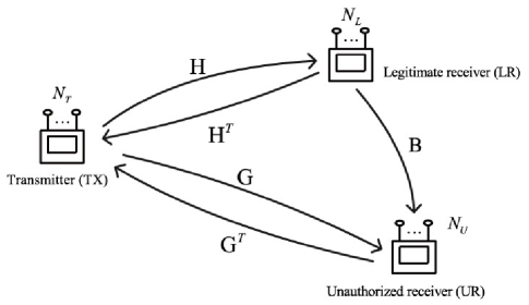
As shown in Fig.1, we consider a wireless MIMO system consisting of a transmitter (TX), a legitimate receiver (LR) and an unauthorized receiver (UR). In the system, the TX, the LR and the UR have $N_{T}$, $N_{L}$, and $N_{U}$ antennas ($N_{T}>N_{L}$), respectively. The TX is connected to one LR and one UR by means of two different communication channels, namely legitimate channel and wiretap channel. The legitimate channel and the wiretap channel are denoted as $\bf{H}\in{\mathbb{C}^{\emph{N}_{\emph{L}}\times\emph{N}_{\emph{T}}}}$, $\bf{G}\in{\mathbb{C}^{\emph{N}_{\emph{U}}\times\emph{N}_{\emph{T}}}}$, respectively. Besides, the channel from the LR to the UR is denoted as $\bf{B}\in{\mathbb{C}^{\emph{N}_{\emph{U}}\times\emph{N}_{\emph{L}}}}$.

Figure 1: A wireless MIMO system includes a multi-antennas transmitter (TX), a multi-antennas legitimate receiver (LR) and a multi-antennas unauthorized receiver (UR).

To enable the LR to interpret the legitimate channel, the TX needs to emit a sequence of training pilots, but this also allows the UR to perform wiretap channel estimation. Therefore, the design of pilot signal is required to ensure a high quality channel estimation at the LR but also prevent the UR from estimating the wiretap channel.
The system model is based on the following assumptions.

1. Channels are assumed to be independently distributed and have reciprocity, e.g., matrix $\bf{H}$ represents downlink legitimate channel and $\bf{H}$^T is uplink legitimate channel. Besides, matrices $\bf{H}$, $\bf{G}$ and $\bf{B}$ are assumed to be the Rayleigh flat fading channels.

2. The entries of channel matrices $\bf{H}$, $\bf{G}$ and $\bf{B}$ are assumed to be i.i.d, $\mathcal{C}\mathcal{N}{(0,\sigma_{\bf{H}}^{2})}$, $\mathcal{C}\mathcal{N}{(0,\sigma_{\bf{G}}^{2})}$ and $\mathcal{C}\mathcal{N}{(0,\sigma_{\bf{B}}^{2})}$, respectively; moreover, the entries of receiver noises are assumed to be the same as independent additive white Gaussian distributed, i.i.d, $\mathcal{C}\mathcal{N}{(0,\sigma_{0}^{2})}$.

The reciprocal assumption indicates that the uplink and downlink channel paths are similar, which happens in time-division duplex (TDD) systems [23]. Such assumption is very critical for the two-way training, and this paper mainly focuses on the design of a DCE scheme in a TDD systems; besides, the Rayleigh flat fading channel assumption indicates that channels are relatively fixed over the transmission of symbols in one time slot but change randomly between time slots. For the second assumption of the system, it refers that the conditions of channels and noises are respectively treated as same for the sake of fair performance.

In this paper, two eavesdropping scenarios are taken into account, that is, passive eavesdropping and active eavesdropping (pilot contamination attack [19]). For the first case, the UR only silently receives signals via channels $\bf{G}$ and $\bf{B}$ during the training phase. For the latter case, the UR not only receives signals but also emits false training pilots from the uplink channel $\bf{G^{\emph{T}}}$ within the training process. Such pilot contamination attack is a potential threat for the two-way training.

II-B The Existing Two-way Training Scheme

The two-way training includes a reverse training phase and a forward training phase. For the reverse training phase, the LR sends a reverse training signal to the TX as

$$\rm{\textbf{S}}_{0}=\sqrt{\frac{\emph{P}_{0}}{\emph{N}_{\emph{L}}}\emph{T}_{0}}\bf{C}_{0}$$ (1)

where $P_{0}$ is the power of the training pilot, and the reverse pilot matrix $\bf{C_{0}}\in\mathbb{C}^{\emph{N}_{L}\times\emph{T}_{1}}$ satisfies an orthogonal condition $\bf{C_{0}C_{0}^{\emph{H}}=I_{\emph{N}_{\emph{L}}}}$. The received signal at the TX is given by

$$\bf{X}_{0}=\bf{H}^{\emph{T}}\bf{S}_{0}+\bf{E}_{0},$$ (2)

where $\bf{E}_{0}\in{\mathbb{C}^{\emph{N}_{\emph{T}}\times\emph{T}_{0}}}$ refers to the AWGN matrix. By employing the linear minimum mean-square error (LMMSE) method [24], the channel estimation at the TX is given by

$$\bf{\hat{H}}_{0}=\sigma^{2}_{H}(\sigma^{2}_{H}S_{0}S^{\emph{H}}_{0}+\sigma^{2}_{0}I_{\emph{N}_{\emph{L}}})^{-1}S_{0}X^{H}_{0}.$$ (3)

In the forward training phase, the TX transmits a sequence of forward training signals inserted with AN to enable channel estimation at the LR while degrading the channel acquisition at the UR. In particular, the AN-aided training sequence, denoted by $\bf{S}_{1}$, has the following expression

$$\bf{S_{1}\triangleq\sqrt{\frac{\emph{P}_{1}}{\emph{N}_{T}}\emph{T}_{1}}C_{1}}+N_{\hat{H}_{{0}}}A,$$ (4)

where $P_{1}$ denotes the power of forward training pilots, $T_{1}$ is the training length, $\bf{C_{1}}\in\mathbb{C}^{\emph{N}_{T}\times\emph{T}_{1}}$ represents the forward pilot matrix which satisfies an orthogonal condition $\bf{C_{1}C_{1}^{\emph{H}}=I_{\emph{N}_{\emph{T}}}}$. Here, $\bf{N_{\hat{H}_{{0}}}}$ is a matrix whose column vectors form an orthogonal basis for the left null space of $\bf{\hat{H}_{{0}}}$, that is, $\bf{N^{\emph{H}}_{\hat{H}_{{0}}}\hat{H}_{{0}}}=0$ and $\bf{N^{\emph{H}}_{\hat{H}_{{0}}}N_{\hat{H}_{{0}}}=I_{\emph{N}_{\emph{T}}-\emph{N}_{\emph{L}}}}$. In addition, $\bf{A\in\mathbb{C}^{(\emph{N}_{\emph{T}}-\emph{N}_{\emph{L}})\times\emph{T}_{1}}}$ is the AN matrix with each component being i.i.d. $\mathcal{C}\mathcal{N}{(0,\sigma_{a}^{2})}$.

The received signals at the LR and the UR are respectively given by

$$\bf{X}_{1}=\bf{H}\bf{S}_{1}+\bf{E}_{1},$$ (5)

$$\bf{Y}_{1}=\bf{G}\bf{S}_{1}+\bf{F}_{1},$$ (6)

where $\bf{E}_{1}\in\mathbb{C}^{\emph{N}_{\emph{L}}\times\emph{T}_{\bf{1}}}$ and $\bf{F}_{1}\in\mathbb{C}^{\emph{N}_{\emph{U}}\times\emph{T}_{1}}$ are the AWGN matrices. By using the LMMSE, the channel estimation at the LR can be expressed as

$$\bf{\hat{H}}_{1}=\sigma^{2}_{H}\{(\sigma^{2}_{H}S_{1}S^{\emph{H}}_{1}+\sigma^{2}_{0}I_{\emph{N}_{\emph{T}}})^{-1}S_{1}X^{H}_{1}\}^{\emph{T}}.$$ (7)

The UR also makes use of the received signals for its channel estimation in the same manner as (7), but the channel performance at the UR would be restricted due to the AN.

III Proposed DCE Scheme under Passive Eavesdropping

III-A Preliminary of Whitening-Rotation based Channel Estimator

We first give a brief introduction of the WR-based semiblind channel approach [20-22]. The channel matrix $\bf{H^{\emph{T}}}$ is firstly estimated in the reverse training phase, so we take the decomposition of channel $\bf{H}^{\emph{T}}$ as an example by

$$\bf{H}^{\emph{T}}={W}{Q}^{\emph{H}},$$ (8)

where $\bf{W}\in{\mathbb{C}^{\emph{N}_{\emph{T}}\times\emph{N}_{\emph{L}}}}$ is a whitening matrix and $\bf{Q}\in{\mathbb{C}^{\emph{N}_{\emph{L}}\times\emph{N}_{\emph{L}}}}$ is an unitary rotation matrix, i.e., $\bf{Q}^{\emph{H}}{Q}={Q}{Q}^{\emph{H}}={I_{\emph{N}_{\emph{L}}}}$. Besides, performing singular value decomposition (SVD) [25] on the channel $\bf{H^{\emph{T}}}$ gives

$$\bf{H}^{\emph{T}}={U}_{{H}^{\emph{T}}}\Sigma_{{H}^{\emph{T}}}{V}_{{H}^{\emph{T}}}^{\emph{H}},$$ (9)

where $\bf{diag(\Sigma_{H})=[\xi_{{1}},...,\xi_{{\emph{N}_{\emph{L}}}}]^{\emph{T}}}$. One possible choice of $\bf{W}$ and $\bf{Q}$ can be $\bf{{U}_{{H}^{\emph{T}}}\Sigma_{{H}^{\emph{T}}}}$ and $\bf{{V}_{{H}^{\emph{T}}}}$, respectively. Without loss of generality, the channel estimation can be divided into two steps with the WR-based semiblind method:

1. Estimate the whitening matrix $\bf{W}$ in a blind fashion using the autocorrelation matrix of the received signals along with a subspace based method.

2. Estimate the unitary rotation matrix $\bf{Q}$ using the training pilots with the constrained maximum likelihood (ML)-based method.

The two-steps of the WR-based channel estimator provides a new training design for improving the DCE performance. Specifically, the WR-based semiblind method can be used for the channel estimation both at the LR and the UR during the two-way training.

III-B Our Proposed WR-based DCE Scheme

III-B1 Step I. reverse training phase

The LR sends the reverse training signals to the TX for the uplink channel estimation without benefiting the channel estimation process at the UR. In the proposed scheme, the design of reverse training signals has the same expression of (1). Different from the existing two-way training, these reverse training signals are randomly generated at the LR and only known by itself, therefore, the TX can not apply the LMMSE method for the channel estimation.
Here, the TX can resort to the blind part of the WR-based semiblind method for the partial acquisition of channel $\bf{H}^{\emph{T}}$. Specifically, we estimate the whitening matrix of $\bf{H}$^T by performing SVD on the autocorrelation matrix of the received signals, which has the following form

$$\bf{{R}}_{\bf{X}_{0}}\triangleq\frac{\bf{X}_{0}\bf{X}_{0}^{\emph{H}}}{\frac{\emph{P}_{0}}{\emph{N}_{\emph{L}}}\emph{T}_{0}}.$$ (10)

Referring to (10), we can estimate the whitening matrix of $\bf{H}$^T as

$$\bf{\hat{W}}_{0}=\frac{1}{\sqrt{\emph{P}_{0}}}U_{{X}_{0}}\Sigma^{\frac{1}{2}}_{{X}_{0}}$$ (11)

by performing SVD on $\bf{R_{X_{0}}}$. By using  (2) , the autocorrelation matrix $\bf{{R}}_{X_{0}}$ can be expressed by

$$\bf{R}_{X_{0}}=H^{\emph{T}}H^{*}+\Delta R_{X_{0}}.$$ (12)

From (12), the error of $\bf{R}_{X_{0}}$ has the following form

$$\bf{\Delta{R}_{X_{0}}=\frac{\emph{N}_{\emph{L}}}{\emph{P}_{0}}(H^{\emph{T}}\Delta{R}_{S_{0},E_{0}}+\Delta{R}^{\emph{H}}_{S_{0},E_{0}}H^{*}+\Delta{R}_{E_{0},E_{0}})},$$ (13)

where the cross correlation matrices $\bf{\Delta{R}_{S_{0},E_{0}}}$,$\bf{\Delta{R}_{E_{0},E_{0}}}$ are defined as follows, respectively

$$\begin{split}\bf{\Delta{R}_{S_{0},E_{0}}}\triangleq\frac{S_{0}E^{\emph{H}}_{0}}{\emph{T}_{0}},\\ \bf{\Delta{R}_{E_{0},E_{0}}}\triangleq\frac{E_{0}E^{\emph{H}}_{0}}{\emph{T}_{0}}.\end{split}$$

Considering the noise interference, the error of the estimated $\bf{\hat{W}_{0}}$ can be defined as

$$\bf{\Delta W_{0}}\triangleq\hat{W}_{0}-W.$$ (14)

By using the results of (8) and (13), $\bf{\Delta{W}_{0}}$ can be deduced as

$$\bf{\Delta W_{0}}=\frac{\emph{N}_{\emph{L}}}{\emph{P}_{0}}\Delta R_{S_{0},{E}_{0}}^{\emph{H}}Q.$$ (15)

III-B2 Step II. forward training phase

For the forward training phase, the design of forward training sequence is required to enable the LR to interpret the downlink channel information but degrade the channel performance at the UR. Here, the new forward training signal is given by

$$\bf{S_{1}\triangleq\sqrt{\frac{\emph{P}_{1}}{\emph{N}_{T}}\emph{T}_{1}}C_{1}}+N_{\hat{W}_{0}}A,$$ (16)

where $\bf{N}_{\hat{W}_{0}}\in\mathbb{C}^{\emph{N}_{L}\times(\emph{N}_{T}-\emph{N}_{L})}$ is the orthogonal complement space matrix of $\bf{\hat{W}_{0}}$ satisfying $\bf{N_{\hat{W}_{0}}^{\emph{H}}\hat{W}_{0}=0}$ and $\bf{N_{\hat{W}_{0}}^{\emph{H}}N_{\hat{W}_{0}}=I_{\emph{N}_{\emph{T}}-\emph{N}_{\emph{L}}}}$. Compared to (4), (16) utilizes the left null space of $\bf{\hat{W}_{0}}$ instead of $\bf{\hat{H}_{0}^{\emph{T}}}$ for the generation of AN. In fact, the left null spaces to the matrices $\bf{{\hat{W}}_{0}}$ and $\bf{{\hat{H}}^{\emph{T}}_{0}}$ are same because the matrix $\bf{{\hat{W}}_{0}}$ has all the eigenvalues of $\bf{{\hat{H}}^{\emph{T}}_{0}}$. We denote the first term of (16) as

$$\bf{\tilde{S}_{1}=\sqrt{\frac{\emph{P}_{1}}{\emph{N}_{T}}\emph{T}_{1}}C_{1}}.$$

The LR may suffer from the the imperfect estimation of $\bf{{W}_{0}}$ due to the interference of AN, thus the power allocation problem between $P_{1}$ and $\sigma^{2}_{a}$ needs to be allocated carefully.

2.1) Channel estimation at the LR: Using (5) and (16), the received signal matrix at the LR can be rewritten as follows

$$\bf{LR:X_{1}=H\tilde{S}_{1}+\tilde{E}_{1}},\\$$ (17)

where

$$\bf{\tilde{E}_{1}\triangleq HN_{\hat{W}_{0}}A+E_{1}}.$$

We apply the WR-based semiblind channel estimator for the channel estimation at the LR. First, the whitening matrix of $\bf{H}$ can be estimated as

$$\bf{{\hat{W}_{1}}=V_{\hat{X}_{W}}^{*}\Sigma^{\emph{T}}_{\hat{X}_{W}}}$$ (18)

by performing SVD on the matrix

$$\bf{\hat{X}_{W}\triangleq\frac{X_{1}\tilde{S}_{1}^{\emph{H}}}{\frac{\emph{P}_{1}}{\emph{N}_{T}}\emph{T}_{1}}},$$ (19)

where

$$\bf{\hat{X}_{W}=U_{\hat{X}_{W}}\Sigma_{\hat{X}_{W}}V_{\hat{X}_{W}}^{\emph{H}}}.$$

After that, the unitary rotation matrix of $\bf{H}$ can be obtained by solving the following optimization problem under the perturbation-free case,

$$\begin{split}&LR:\ \ minf(\bf{Q})=\bf{\sum\limits_{\emph{i}=1}^{\emph{N}_{\emph{L}}}\parallel X_{1}(\emph{i})-\sum\limits_{\emph{j}=1}^{\emph{N}_{\emph{T}}}\hat{\sigma}_{\emph{j}}\emph{q}_{\emph{ij}}^{*}\hat{S}_{1}(\emph{j})\parallel^{2}_{\emph{F}}}\\ &\bf{s.t.\indent QQ^{\emph{H}}=I_{\emph{N}_{\emph{L}}}},\end{split}$$ (20)

where $\bf{\hat{S}_{1}=V^{\emph{H}}_{X_{W}}\tilde{S}_{1}}$, $\bf{X_{1}(\emph{i})}$ represents the $i$th column of $\bf{X_{1}}$ and $\bf{\hat{S}_{1}}(\emph{j})$ refers to the $j$th column of $\bf{\hat{S}_{1}}$, respectively. By using the Lagrange method (the derivation can be found in appendix A), the unitary rotation matrix can be calculated as follows

$$\bf{\hat{Q}_{1}=U_{\hat{X}_{Q}}V_{\hat{X}_{Q}}^{\emph{H}}}$$ (21)

by performing SVD on the matrix

$$\bf{\hat{X}_{Q}\triangleq\frac{X_{1}^{*}\tilde{S}_{1}^{\emph{T}}\hat{W}_{1}}{\frac{\emph{P}_{1}}{\emph{N}_{\emph{T}}}\emph{T}_{1}}},$$ (22)

where

$$\bf{\hat{X}_{Q}=U_{\hat{X}_{Q}}\Sigma_{\hat{X}_{Q}}V_{\hat{X}_{Q}}^{\emph{H}}}.$$

According to (8), the legitimate channel $\bf{H}$ can be calculated by $\bf{\hat{H}_{1}=\hat{Q}_{1}^{\texttt{*}}\hat{W}^{\emph{T}}_{1}}$.

2.2) Channel estimation at UR: Likewise, the wiretape channel $\bf{G}$ can be decomposed as

$$\bf{G=MR^{\emph{H}}},$$ (23)

where $\bf{M}\in{\mathbb{C}^{\emph{N}_{\emph{U}}\times\emph{N}_{\emph{T}}}}$ is the whitening matrix, and $\bf{R}\in{\mathbb{C}^{\emph{N}_{\emph{T}}\times\emph{N}_{\emph{T}}}}$ is the unitary rotation matrix. Besides, $\bf{G}$ can be decomposed by SVD as follows

$$\bf{G=U_{G}\Sigma_{G}V^{\emph{H}}_{G}},$$ (24)

where $\bf{diag(\Sigma_{G})=[\gamma_{{1}},...,\gamma_{{\emph{N}_{\emph{U}}}}]^{\emph{T}}}$. Without loss of generality, we can assume that $\bf{M=U_{G}\Sigma_{G}}$ and $\bf{R=V_{G}}$.

When the UR employs the WR-based semiblind channel estimator for its channel estimation, the received signal matrix of (6) can be rewritten as follows

$$\bf{UR:Y_{1}=G\tilde{S}_{1}+\tilde{F}_{1}},\\$$ (25)

where $\bf{\tilde{F}_{1}\triangleq GN_{\hat{W}_{0}}A+F_{1}}$. Then, the whitening matrix of $\bf{G}$ can be obtained as

$$\bf{\hat{M}=U_{\hat{Y}_{M}}\Sigma_{\hat{Y}_{M}}}$$ (26)

by performing SVD to the matrix

$$\bf{\hat{Y}_{M}\triangleq\frac{Y_{1}\tilde{S}_{1}^{\emph{H}}}{\frac{\emph{P}_{1}}{\emph{N}_{\emph{T}}}\emph{T}_{1}}},$$ (27)

where

$$\bf{\hat{Y}_{M}=U_{\hat{Y}_{M}}\Sigma_{\hat{Y}_{M}}V_{\hat{Y}_{M}}^{\emph{H}}}.$$

Next, the rotation matrix of $\bf{G}$ can be calculated using the training-based method [22],

$$\bf{\hat{R}=V_{\hat{Y}_{R}}U_{\hat{Y}_{R}}^{\emph{H}}}$$ (28)

by performing SVD to the matrix

$$\bf{\hat{Y}_{R}\triangleq\frac{\hat{M}^{\emph{H}}Y_{1}\tilde{S}_{1}^{\emph{H}}}{\frac{\emph{P}_{1}}{\emph{N}_{\emph{T}}}\emph{T}_{1}}},$$ (29)

where

$$\bf{\hat{Y}_{R}=U_{\hat{Y}_{R}}\Sigma_{\hat{Y}_{R}}V_{\hat{Y}_{R}}^{\emph{H}}}.$$

Using (26) and (28), the wiretap channel $\bf{G}$ can be calculated by $\bf{\hat{G}=\hat{M}\hat{R}^{\emph{H}}}$.

III-C DCE Performance Analysis

We mainly discuss the DCE performance in this Section. A quantitative analysis of power allocation is offered for the optimal DCE scheme.

III-C1 Channel estimation performance at the LR

To analyze channel estimation performance, we define the perturbation errors of $\bf{\hat{W}_{1}}$ and $\bf{\hat{Q}_{1}}$, i.e., $\bf{\Delta{W}_{1}}\triangleq\hat{W}_{1}-W$ and $\bf{\Delta{Q}_{1}}\triangleq\hat{Q}_{1}-Q$. The estimation error of $\bf{H}$ at the LR is given by

$$\bf{\Delta H_{1}}\triangleq\hat{H}_{1}-H=\hat{Q}^{*}\hat{W}^{\emph{T}}_{1}-Q^{*}W^{\emph{T}}_{1}\approx Q^{*}\Delta W^{\emph{T}}_{1}+\Delta Q_{1}^{*}W^{\emph{T}}.$$ (30)

First, we derive the closed-form expression of $\bf{\Delta{{W}_{1}}}$. Similar to (15), $\bf{\Delta{W}_{1}}$ has the following expression

$$\bf{\Delta{{W}_{1}}=\frac{\emph{N}_{\emph{T}}}{\emph{P}_{1}}Q^{\emph{T}}\Delta R^{*}_{\tilde{S}_{1},\tilde{E}_{1}}},$$ (31)

where

$$\begin{split}\bf{\Delta R_{\tilde{S}_{1},\tilde{E}_{1}}=\Delta R_{\tilde{S}_{1},E_{1}}+\Delta R_{\tilde{S}_{1},A}N^{\emph{{H}}}_{\hat{W}_{0}}H^{\emph{H}}}.\end{split}$$

Notice that $\bf{N^{\emph{T}}_{\hat{W}_{0}}\hat{W}_{0}=0}$, (31) can be rewritten as

$$\begin{split}\bf{\Delta{{W}_{1}}=\frac{\emph{N}_{\emph{T}}}{\emph{P}_{1}}Q^{\emph{T}}(\Delta R_{\tilde{S}_{1},E_{1}}^{*}-\frac{1}{\emph{P}_{0}}\Delta R_{\tilde{S}_{1},A}^{*}N^{\emph{T}}_{\hat{W}_{0}}\Delta R^{\emph{H}}_{S_{0},E_{0}})}.\end{split}$$ (32)

Next, we deduce the closed-form expression of $\bf{\Delta Q_{1}}$. Using the result of [22], $\bf{\Delta{Q}_{1}}$ equals to

$$\bf{\Delta{Q}_{1}\approx Q(\Gamma_{Q}\circ\Pi_{Q})^{\emph{H}}},$$ (33)

where

$$\begin{split}\bf{\Gamma_{Q}}=\begin{bmatrix}\frac{1}{2{\xi}_{1}^{2}},&...&,\frac{1}{{\xi}_{1}^{2}+{\xi}_{\emph{N}_{\emph{L}}}^{2}}&\\ \frac{1}{{\xi}_{2}^{2}+{\xi}_{1}^{2}},&...&,\frac{1}{{\xi}_{2}^{2}+{\xi}_{\emph{N}_{\emph{L}}}^{2}}\\ &....&\\ \frac{1}{{\xi}_{{\emph{N}_{\emph{L}}}}^{2}+{\xi}_{{1}}^{2}},&...&,\frac{1}{2{\xi}_{{\emph{N}_{\emph{L}}}}^{2}}&\end{bmatrix}\end{split}$$ (34)

and

$$\begin{split}&\bf{\Pi_{Q}=\Delta X_{Q}^{\emph{H}}Q-Q^{\emph{H}}\Delta X_{Q}}.\end{split}$$ (35)

To derive the perturbation error of $\bf{\Delta X_{Q}}$, we define $\bf{\hat{X}_{Q}\triangleq X_{Q}+\Delta X_{Q}}$. Using (5), (22) can be modified as

$$\begin{split}&\bf{\hat{X}_{Q}=H^{*}W+H^{*}\Delta W_{1}+\frac{\emph{N}_{\emph{T}}}{\emph{P}_{1}}\Delta R^{\emph{T}}_{\tilde{S}_{1},\tilde{E}_{1}}W}.\end{split}$$ (36)

Therefore, we have

$$\bf{\Delta X_{Q}=H^{*}\Delta W_{1}+\frac{\emph{N}_{\emph{T}}}{\emph{P}_{1}}\Delta R^{\emph{T}}_{\tilde{S}_{1},\tilde{E}_{1}}W}.$$ (37)

Substituting (37) into (35) , we have

$$\begin{split}&\bf{\Pi_{Q}}=0.\end{split}$$ (38)

As a result, (33) can be summarized as $\bf{\Delta Q_{1}}=0$, and the perturbation error of $\bf{\hat{H}_{1}}$ is given by

$$\begin{split}&\bf{\Delta H_{1}=\frac{\emph{P}_{1}}{\emph{N}_{\emph{T}}}(\Delta R_{\tilde{S}_{1},E_{1}}^{*}-\frac{\emph{N}_{\emph{L}}}{\emph{P}_{0}}\Delta R_{\tilde{S}_{1},A}^{*}N^{\emph{T}}_{\hat{W}_{0}}\Delta R^{\emph{H}}_{S_{0},E_{0}})}.\end{split}$$ (39)

Similar to the derivation of [22], the NMSE criterion like [24] of the estimated matrix $\bf{{H}}$ at the LR is given by

$$\begin{split}&\bf{NMSE}_{\emph{L}}\triangleq\frac{\rm{Tr}(E\{\bf{\Delta H_{1}\Delta H_{1}^{\emph{H}}\}})}{\emph{N}_{\emph{L}}\emph{N}_{\emph{T}}}\\ &=\frac{\emph{N}_{\emph{T}}\sigma_{0}^{2}}{\emph{P}_{1}\emph{T}_{1}}+\frac{\emph{N}_{\emph{L}}(\emph{N}_{\emph{T}}-\emph{N}_{\emph{L}})\sigma^{2}_{\emph{a}}}{\emph{P}_{0}\emph{T}_{0}}\frac{\emph{N}_{\emph{T}}\sigma^{2}_{0}}{\emph{P}_{1}\emph{T}_{1}}.\end{split}$$ (40)

III-C2 Channel estimation performance at the UR

We define the perturbation errors of $\bf{\hat{M}}$ and $\bf{\hat{R}}$, i.e., $\bf{\Delta{M}}\triangleq\hat{M}-M$ and $\bf{\Delta{R}}\triangleq\hat{R}-R$. In the following, the estimation error of channel $\bf{G}$ can be given by

$$\begin{split}&\bf{\Delta G}\triangleq\hat{G}-G=\hat{M}\hat{R}^{\emph{H}}-MR^{\emph{H}}\approx M\Delta R^{\emph{H}}+\Delta MR^{\emph{H}}.\end{split}$$ (41)

First, we derive the closed-form expression of $\bf{\Delta M}$. Similar to (15), $\bf{\Delta M}$ has the following expression

$$\bf{\Delta M=\frac{\emph{N}_{\emph{T}}}{\emph{P}_{1}}\Delta R^{\emph{H}}_{\tilde{S}_{1},\tilde{F}_{1}}R},$$ (42)

where

$$\begin{split}\bf{\Delta R_{\tilde{S}_{1},\tilde{F}_{1}}\triangleq\Delta R_{\tilde{S}_{1},A}N^{\emph{H}}_{\hat{W}_{0}}G^{\emph{H}}+\Delta R_{\tilde{S}_{1},F_{1}}}.\end{split}$$

Next, we deduce the closed-form expression of $\bf{\Delta R}$. Similar to (33), the perturbation matrix of $\bf{\hat{R}}$ is given by

$$\bf{\Delta{R}\approx R(\Gamma_{R}\circ\Pi_{R})},$$ (43)

where $\bf{\Gamma_{R}}$ is

$$\begin{split}\bf{\Gamma_{R}}=\begin{bmatrix}\frac{1}{2{\gamma}_{1}^{2}},&...&,\frac{1}{{\gamma}_{1}^{2}+{\gamma}_{\emph{N}_{\emph{U}}}^{2}}&\\ \frac{1}{{\gamma}_{2}^{2}+{\gamma}_{1}^{2}},&...&,\frac{1}{{\gamma}_{2}^{2}+{\gamma}_{\emph{N}_{\emph{U}}}^{2}}\\ &....&\\ \frac{1}{{\gamma}_{{\emph{N}_{\emph{U}}}}^{2}+{\gamma}_{{1}}^{2}},&...&,\frac{1}{2{\gamma}_{{\emph{N}_{\emph{U}}}}^{2}}&\end{bmatrix}\end{split}$$ (44)

and

$$\begin{split}&\bf{\Pi_{R}=R^{\emph{H}}\Delta Y^{\emph{H}}_{R}-\Delta Y_{R}R}.\end{split}$$ (45)

To derive the perturbation error matrix $\bf{\Delta Y_{R}}$, we define $\bf{\hat{Y}_{R}\triangleq Y_{R}+\Delta Y_{R}}$. Using (6), (29) can be approximately by

$$\begin{split}&\bf{\hat{Y}_{R}\approx M^{\emph{H}}G+\Delta M^{\emph{H}}G+\frac{\emph{N}_{T}}{\emph{P}_{1}}M^{\emph{H}}\Delta R^{\emph{H}}_{\tilde{S}_{1},\tilde{F}_{1}}},\end{split}$$ (46)

Therefore,

$$\begin{split}&\bf{\Delta Y_{R}=\Delta M^{\emph{H}}G+\frac{\emph{N}_{\emph{T}}}{\emph{P}_{1}}M^{\emph{H}}\Delta R^{\emph{H}}_{\tilde{S}_{1},\tilde{F}_{1}}}.\end{split}$$ (47)

Substituting (47) into (45), we have $\bf{\Pi_{R}=0}$. As a result, (43) can be summarized as $\bf{\Delta R=0}$. Then, the perturbation matrix of $\bf{\hat{G}}$ can be yielded as

$$\begin{split}&\bf{\Delta G=\frac{\emph{N}_{\emph{T}}}{\emph{P}_{1}}(GN_{\hat{W}_{0}}\Delta R_{\tilde{S}_{1},A}+\Delta R_{\tilde{S}_{1},F_{1}})}.\end{split}$$ (48)

In consequence, the NMSE criterion of estimated $\bf{{G}}$ at the UR can be derived by

$$\begin{split}&\bf{NMSE}_{\emph{U}}\triangleq\frac{\rm{Tr}(E{\bf{\{\Delta{G}\Delta{G}^{\emph{H}}}\}})}{\emph{N}_{\emph{T}}\emph{N}_{\emph{U}}}\\ &=\frac{\emph{N}_{\emph{T}}\sigma_{0}^{2}+\emph{N}_{\emph{T}}(\emph{N}_{\emph{T}}-\emph{N}_{\emph{L}})\sigma_{\emph{a}}^{2}\sigma_{G}^{2}}{\emph{P}_{1}\emph{T}_{1}}.\end{split}$$ (49)

Comparing (40) and (49), we find that the NMSE performance at the LR and the UR are mainly relevant to the selection of power values among the training pilots and AN. When the power of training pilots becomes stronger, the precision of the channel estimation is higher for the LR but lower for the UR. Alternatively, the estimation precision is lower for the LR while higher for the UR when the power of training pilots becomes lower. Therefore, a power allocation trade-off exists between the training pilots and AN.

III-C3 Optimal Power Allocation between the Training Pilots and AN

One needs to allocate the available power between the training pilots and the AN carefully through minimizing the channel estimation error at the LR while restricting the estimation error at the UR. We formulate the power allocation as the following optimization problem

$$\min\limits_{P_{0},P_{1}>0,\sigma_{a}^{2}\geqslant 0}~{}\bf{NMSE}_{\emph{L}}$$ (50)

$$s.t.\quad\bf{NMSE}_{\emph{U}}\geq\gamma,$$ (51a)

$$~{}~{}\quad P_{0}\leq P_{ave}$$ (52a)

$$P_{1}+(N_{T}-N_{L})\sigma_{a}^{2}\leq P_{ave},$$ (53a)

where $\gamma>0$ refers to the threshold of the UR’s achievable NMSE, and $P_{ave}$ is the total energy constraint of the training signal. We define $x=\frac{P_{1}T_{1}}{N_{T}},y=(N_{T}-N_{L})\sigma_{a}^{2}$, $z=P_{0}$. Then, the problem (50) can be reformulated as

$$\min\limits_{x>0,y\geq 0}~{}\frac{\sigma_{0}^{2}}{x}+\frac{yN_{L}\sigma^{2}_{0}}{xz}$$ (54)

$$s.t.~{}~{}\frac{\sigma_{0}^{2}}{x}+\frac{y\sigma_{G}^{2}}{x}\geq\gamma,$$ (55a)

$$~{}~{}~{}\quad z\leq P_{ave},$$ (56a)

$$\frac{xN_{T}}{T_{1}}+y\leq P_{ave}.$$ (57a)

The problem (54) is a convex optimization problem involving three variables $(x,y,z)$. We will prove that the three-dimensional optimization problem can be solved by a simple one-dimensional line search [26]. (The proof can be found in the Appendix B.)

• Proposition 1. Let $\{x^{*},y^{*},z^{*}\}$ be the optimal solution to the convex optimization problem in (54) with the constraint that $\frac{N_{T}\sigma^{2}_{0}}{P_{ave}T_{1}}\leq\gamma\leq(N_{T}-N_{L})P_{ave}$. The optimal value of $x$ can be solved by the following one-dimensional optimization problem

  $$\min\limits_{x}~{}~{}~{}~{}\frac{\sigma_{0}^{2}}{x}+\frac{y(x)N_{L}\sigma^{2}_{0}}{xz}$$ (58)

  $$s.t.~{}~{}~{}\frac{\sigma^{2}_{0}}{\gamma}\leq x\leq\frac{(\sigma^{2}_{G}P_{ave}+\sigma^{2}_{0})T_{1}}{\gamma T_{1}+N_{T}\sigma^{2}_{G}},$$ (59a)

  where

  $$\begin{split}&y(x^{*})=\frac{x\gamma-\sigma^{2}_{0}}{\sigma^{2}_{G}},\\ &z^{*}=P_{ave}.\end{split}$$

  The associated values of $y^{*}$,$z^{*}$ are given by $y(x^{*})$, $P_{ave}$, respectively.

With the result of Proposition 1, we can construct well designed training sequences for achieving optimal DCE performance.

IV Proposed DCE Scheme under the Pilot Contamination Attack

In this Section, we analyze the performance of our proposed DCE scheme under the pilot contamination attack.

IV-A The Existing Pilot Contamination Attack

Under the existing two-way training scheme, the pilot contamination attack is possible when the reverse training pilots are known by the UR. Notice that the publicly known reverse training pilots provide an opportunity for the UR to make an adverse influence on the channel estimation at the TX. In particular, the UR sends the reverse training pilots at the same time as the LR’s transmission during the reverse training phase. With the additive AWGN matrix $\bf{F}_{0}\in{\mathbb{C}^{\emph{N}_{\emph{T}}\times\emph{T}_{0}}}$, the received signals at the TX are given by

$$\bf{X}_{0}=\bf{H}^{\emph{T}}S_{0}+\bf{E}_{0}+G^{\emph{T}}\bar{S}_{0}+F_{0},$$ (60)

where

$$\bf{\bar{S}_{0}=\sqrt{\frac{{\bar{\emph{P}}}_{0}}{\emph{N}_{\emph{L}}}\emph{T}_{0}}\bar{C}_{0}},$$

$\bar{P}_{0}$ is the power of injected fake pilot and pilot matrix $\bar{C}_{0}$ satisfies that $\bf{\bar{C}_{0}\bar{C}_{0}^{\emph{H}}=I_{\emph{N}_{\emph{L}}}}$. If the UR knows the reverse training pilot, then ${{{\bar{P}}}}_{0}=P_{0}$ and ${{{\bar{C}}}}_{0}=C_{0}$. For simplicity, we define the injected noises of (60) as

$$\bar{\bf{F}}_{0}\triangleq\bf{G}^{\emph{T}}\bar{S}_{0}+\bf{F}_{0}.$$ (61)

The pilot contamination attack can be viewed as a form of malicious signal injection. With the injection of false training pilot, the UR can degrade the TX’s estimation of uplink channel $\bf{H^{\emph{T}}}$ and also align the wiretap channel estimation for the UR. In conclusion, the impact of the pilot contamination attack on the two-way DCE scheme has two folds: it reduces the accuracy of the LR’s estimation of the downlink channel due to the leakage of AN; and more seriously it increases the UR’s channel performance.

IV-B The Impact of Pilot Contamination Attack on the Proposed Scheme

For our proposed two-way training, the reverse training pilots are randomly generated at the LR and only known by itself. Therefore, the randomness feature of the reverse training pilots provides a natural way of protecting against the pilot contamination attack. Possibly, the UR may try to exploit the received signals from channel $\bf{B}$ via the blind detection methods [27,28]. However, the UR would suffer from a rotation ambiguity between the estimated channel $\bf{\hat{B}}$ and channel $\bf{{B}}$. Therefore, it is still no use for the UR to interpret the reverse training pilot without the cooperation of the LR.
Here, we consider a scenario when the UR performs pilot contamination attack with a guessing-based way, that is, the pilots $\bf{\bar{C}_{0}}$ is randomly generated by a guess way. We employ the WR-based semiblind channel estimator for the DCE performance. In order to study such attack, we mainly focus on its impact on the NMSE performance of the estimated channel $\bf{\hat{H}_{1}}$ at the LR. By using (31), the perturbation error of the whitening matrix to the estimated channel $\bf{\hat{H}_{1}}$ can be rewritten as

$$\bf{\Delta{{W}_{1}}=\frac{\emph{N}_{\emph{T}}}{\emph{P}_{1}}Q^{\emph{T}}\Delta R^{*}_{\tilde{S}_{1},{\tilde{E}}_{1}}},$$ (62)

where

$$\begin{split}&\bf{\Delta R_{\tilde{S}_{1},\tilde{E}_{1}}\approx}\\ &\bf{\Delta R_{\tilde{S}_{1},E_{1}}-\frac{\emph{N}_{\emph{L}}}{\emph{P}_{0}}\Delta R_{\tilde{S}_{1},A}N^{\emph{H}}_{\hat{W}_{0}}(\Delta R^{\emph{T}}_{S_{0},{E}_{0}}+\Delta R^{\emph{T}}_{S_{0},\bar{F}_{0}})}.\end{split}$$

Similar to (33), the perturbation error of the unitary rotation matrix can be deduced as $\bf{\Delta Q_{1}}=0$. Hence, the perturbation error of the estimated channel $\bf{\hat{H}_{1}}$ is given by

$$\begin{split}&\bf{\Delta H_{1}}=\\ &\frac{\emph{P}_{1}}{\emph{N}_{\emph{T}}}\{\Delta R_{\tilde{S}_{1},E_{1}}^{*}-\frac{\emph{N}_{\emph{L}}}{\emph{P}_{0}}\Delta R_{\tilde{S}_{1},A}^{*}N^{\emph{T}}_{\hat{W}_{0}}(\Delta R^{\emph{H}}_{S_{0},E_{0}}+\Delta R^{\emph{H}}_{S_{0},\bar{F}_{0}})\}.\end{split}$$ (63)

With the result of (63), the NMSE criterion of the estimated channel $\bf{H_{1}}$ at the LR is given by

$$\begin{split}&\bf{NMSE}_{\emph{L}}\approx\frac{\emph{N}_{\emph{T}}\sigma^{2}_{0}}{\emph{P}_{1}\emph{T}_{1}}+\frac{\emph{N}_{\emph{L}}(\emph{N}_{\emph{T}}-\emph{N}_{\emph{L}})\sigma^{2}_{\emph{a}}}{\emph{P}_{0}\emph{T}_{0}}\frac{\emph{N}_{\emph{T}}\sigma^{2}_{0}}{\emph{P}_{1}\emph{T}_{1}}\\ &+\frac{\emph{N}_{\emph{L}}(\emph{N}_{\emph{T}}-\emph{N}_{\emph{L}})\sigma^{2}_{\emph{a}}}{\emph{P}_{1}\emph{T}_{1}}(\frac{\emph{N}_{\emph{T}}\sigma^{2}_{0}}{\bar{\emph{P}}_{0}\emph{T}_{0}}+\frac{\emph{N}_{\emph{U}}\sigma^{2}_{G}}{{\emph{P}}_{0}\emph{T}_{0}}).\end{split}$$ (64)

When we compare (64) and (40), the third term of (64) is newly introduced due to the injection of fake training pilot. The third term is significantly smaller than the first of two terms. Therefore, the pilot contamination attack only marginally increases the NMSE error at the LR. Furthermore, (64) demonstrates that the power allocation using Proposition 1 is still valid under the pilot contamination attack.

V Numerical results

We consider a MIMO wireless system with one LR and one UR. In the system, we have $N_{T}=4,N_{L}=2$ and $N_{U}=2$. Channel matrices $\bf{H}$ or $\bf{G}$ are i.i.d. complex Gaussian random variables with zero mean and unit variance ($\bf{\sigma^{2}_{H}=\sigma^{2}_{G}=1}$); and the additive noise matrices $\bf{E_{0}}$, $\bf{E}_{1}$ or $\bf{F}_{1}$ are i.i.d. AWGN ($\sigma^{2}_{0}=0.01$). We set the maximum transmission power as 30 dBm, i.e., $P_{ave}=1$. The reverse training pilot matrix and the forward pilot matrix satisfy that $\bf{C_{0}C_{0}^{\emph{H}}=I_{\emph{N}_{\emph{L}}}}$, $\bf{C_{1}C_{1}^{\emph{H}}=I_{\emph{N}_{\emph{T}}}}$, respectively. Moreover, the overall training length is given as $T=280$, in which $T_{0}=T_{1}=140$. The parameter $\gamma$ is set as 0.03 or 0.1 [17]. With $P_{ave}=1$, the criterion of signal-to-noise ratios (SNRs) at the LR and the UR can be defined as

$$\begin{split}\bf{SNR}_{\emph{L}}=\frac{\rm{E}\bf{\parallel HS_{1}\parallel_{\emph{F}}^{2}}}{\rm{E}\bf{\parallel E_{1}\parallel_{\emph{F}}^{2}}}=\frac{1}{\sigma_{0}^{2}},\\ \bf{SNR}_{\emph{U}}=\bf{\frac{\rm{E}{\parallel\bf{GS}_{1}\parallel_{\emph{F}}^{2}}}{\rm{E}{\parallel\bf{F}_{1}\parallel_{\emph{F}}^{2}}}}=\frac{1}{\sigma_{0}^{2}},\\ \end{split}$$ (65)

where $\bf{SNR}_{\emph{L}}=\bf{SNR}_{\emph{U}}$. Here, the DCE scheme based on the LMMSE channel estimator in [18] is employed as a fair comparison to the proposed DCE scheme based on the WR channel estimator. In the following, the scheme in [18] is called as LMMSE-based DCE scheme, and the proposed scheme is named as WR-based DCE scheme. The result of each DCE scheme is obtained over 100,000 Monte Carlo running.

Figure 2: Power allocation among the training signals and AN in our proposed DCE scheme

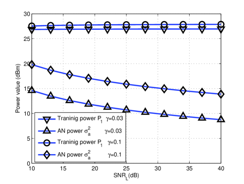
We first demonstrate the efficiency of the proposed DCE scheme. Both the LR and the UR exploit their channel estimation with the received signal samples. The optimal power value among $P_{1}$ and $\sigma^{2}_{a}$ can be calculated via the optimized solution of (58). Fig.2 shows that more power is needed for the forward training pilots than the AN at all SNR levels. There is a minor variation between the powers of forward training pilots and the AN at all SNR levels. This observation indicates that the power allocation solution has a stable performance.
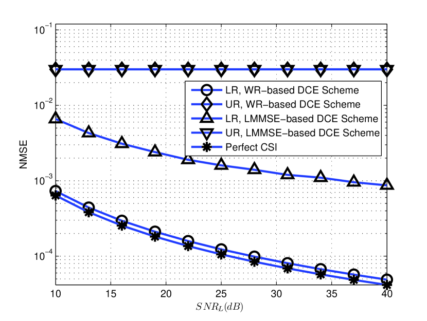
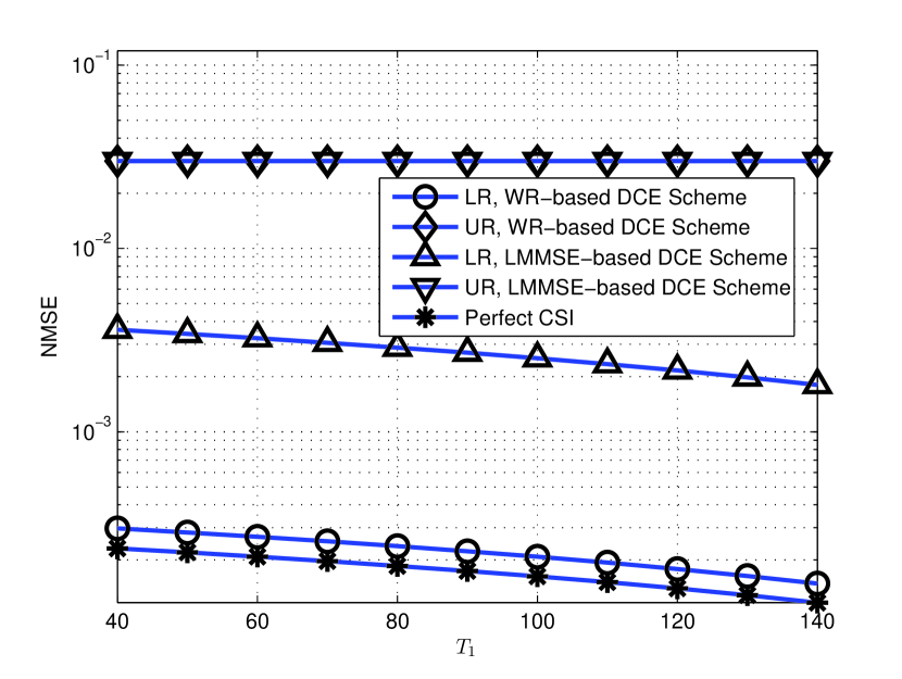
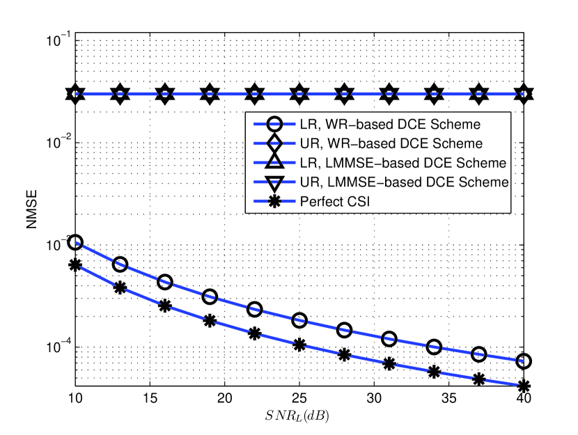
From Fig.3 (a) and Fig.3 (b), it is found that the NMSE performance at the LR with the WR-based DCE scheme achieves better DCE performance than the LMMSE-based DCE scheme. By assuming that the TX knows perfect CSI of the uplink channel, we illustrate the ideal lower bound of NMSE with the proposed DCE scheme in the figures. The gap between the ideal lower bound with perfect CSI and the NMSE error at the LR with the LMMSE-based DCE scheme is wide while it is very close to the WR-based DCE scheme. Furthermore, Fig 3.(c) shows the relationship between NMSE at the LR and the training sequence length. The NMSE performance at the LR improves the DCE performance with longer training pilots. Although our simulation results are shown for the scenario where the LR and UR are at the same distance from the TX ($\bf{\sigma^{2}_{H}=\sigma^{2}_{G}}$), the proposed DCE scheme works well even if the UR is much closer to the TX as long as the transmit power is sufficiently large. The reason is that the SNR at the UR does not change much with distance when the inserted AN dominates the noise at the UR.

(a) $\gamma=0.03$

(b) $\gamma=0.1$

(c) Variation of $T_{1}$ when $SNR_{L}=25dB$.

Figure 3: NMSE performance comparison between the LMMSE-based DCE scheme and the WR-based DCE scheme

(a) $\gamma=0.03$

(b) $\gamma=0.1$

(c) Variation of $\bar{P}_{0}$ when the noise levels are set as $15dB$, $25dB$, $35dB$, respectively.

Figure 4: NMSE performance of the LMMSE-based DCE scheme and the WR-based DCE scheme under the pilot contamination attack

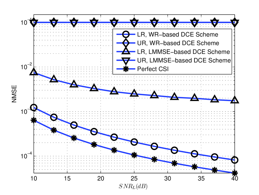
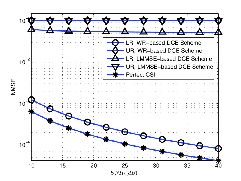
We then look into the performance of the proposed WR-based DCE scheme under a pilot contamination attack. As we have discussed in Section IV, the UR has no knowledge of the reverse training signals. In addition, we suppose that the UR sends another guess-based orthogonal signals $\bf{\bar{S}}_{0}$ to attack the system, in which $\bar{P}_{0}=P_{ave}=1$. From Fig.4 (a), one can see that the NMSE performance at the LR with LMMSE-based DCE scheme has approximately reached the limitation of the UR’s NMSE due to the poor channel estimation. On the contrary, the NMSE performance at the LR with the proposed DCE scheme only has a slight reduction. Similar results can be observed in Fig.4 (b) in case of $\gamma=0.1$. As a result, the LMMSE-based DCE scheme is more sensitive to the pilot contamination attack than our proposed DCE scheme.

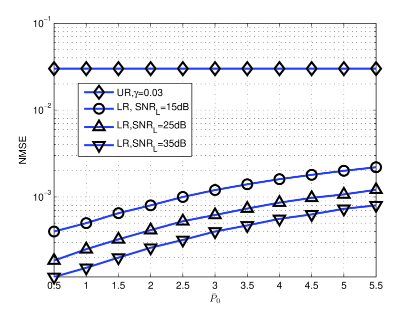
Fig.4 (c) shows the impact of pilot contamination attack on the performance of our proposed scheme with variation of attack power. Since the LMMSE-based DCE scheme works not very well under the pilot contamination attack, we only focus on the performance of the proposed DCE scheme. The result show that the obtained NMSE error at the LR has a slight reduction with the increasing power $\bar{P}_{0}$. The attack power is restricted at the UR, hence the pilot contamination attack has an ignorable impact on the performance of our proposed DCE scheme.

VI Conclusion

In this paper, we proposed a new two-way training scheme for DCE in wireless MIMO systems. To improve the DCE performance, an efficient whitening-rotation (WR) based semiblind approach has been employed in the two-way training. A closed-form of NMSE on the channel estimation between the LR and the UR has been developed, facilitating optimal power allocation between the training signals and AN. Furthermore, the proposed training design offers a countermeasure against the pilot contamination attack. It has been proved that the pilot contamination attack has a very limited impact on the DCE performance. Simulation results demonstrate that our proposed scheme can achieve higher performance than the existing training scheme.
Our future work includes the following directions of research: (a) We will extend the study of DCE from narrowband systems to wideband OFDM-based systems [29]. The power allocation between the training signal and AN across all pilot subcarriers will be an interesting problem to investigate. (b) We will apply the semiblind two-way training method to tackle the pilot contamination problem in multi-cell massive MIMO systems.

Appendix A Derivation of unitary rotation matrix

According to (20), the rotation matrix $\bf{Q}$ can be obtained by using Lagrange method as follows,

$$\begin{split}&LR:\ \ minf(\bf{Q},\lambda,\mu)=\sum\limits_{\emph{i}=1}^{\emph{N}_{\emph{L}}}\parallel\bf{X_{1}(\emph{i})}-\sum\limits_{\emph{j}=1}^{\emph{N}_{\emph{T}}}\hat{\sigma}_{\emph{j}}\emph{q}_{\emph{ij}}^{*}\bf{\hat{S}}_{1}(\emph{j})\parallel_{\emph{F}}^{2}\\ &+\sum\limits_{i=1}^{\emph{N}_{L}}Re\{\lambda_{i}(q^{\emph{H}}_{\emph{i}}q_{i}-1)\}+\sum\limits_{i=1}^{N_{L}}\sum\limits_{j=i+1}^{N_{L}}Re\{\mu_{ij}q^{H}_{i}q_{j}\}.\end{split}$$ (66)

By differentiating (66) w.r.t $\bf{Q}$ and let it equals to $0$, we have

$$\bf{X_{1}^{*}\tilde{S}_{1}^{\emph{T}}\hat{W}_{1}-Q\hat{W}_{1}^{\emph{T}}\tilde{S}_{1}\tilde{S}^{\emph{H}}_{1}\hat{W}_{1}=Q\Theta},$$ (67)

where $\Theta$ is the matrix of Lagrange multipliers which satisfies $\Theta_{ii}=\lambda_{i}$,$\Theta_{ij}=\mu_{ij}$ when $i>j$ and $\Theta_{ij}=\mu^{*}_{ij}$ when $i<j$. We divide $\frac{\emph{P}_{1}}{\emph{N}_{\emph{T}}}\emph{T}_{1}$ on both sides of (67), and denote

$$\bf{\hat{X}_{Q}\triangleq\frac{X_{1}^{*}\hat{S}_{1}^{\emph{T}}\hat{W}_{1}}{\frac{\emph{P}_{1}}{\emph{N}_{\emph{T}}}\emph{T}_{1}}}.$$

Using the conjugate symmetry feature of $\Theta$, we premultiply $\bf{Q}^{\emph{H}}$ to (67) and post-multiply $\bf{Q}^{\emph{H}}$ to the conjugate of (67). Performing a subtraction between the two new equations, we have

$$\bf{Q^{\emph{H}}\hat{X}_{Q}=\hat{X}_{Q}^{\emph{H}}Q}.$$ (68)

According to the specific structure of (68), it holds if and only if

$$\begin{split}\bf{\hat{Q}_{1}=U_{\hat{X}_{Q}}V_{\hat{X}_{Q}}^{\emph{H}}},\end{split}$$ (69)

where $\bf{U_{\hat{X}_{Q}}}$ and $\bf{V_{\hat{X}_{Q}}}$ are the decomposition results after performing SVD on $\bf{\hat{X}_{Q}}$, e.g., $\bf{\hat{X}_{Q}=U_{\hat{X}_{Q}}\Sigma_{\hat{X}_{Q}}V_{\hat{X}_{Q}}^{\emph{H}}}$.

Appendix B Derivation of optimum power allocation

First, we need to develop the range of parameter $\gamma$. For the extreme case when $y=0$, we know that

$$\centering\begin{split}x\leq\frac{P_{ave}T_{1}}{N_{T}}\end{split}\@add@centering$$ (70)

by using the power constraint of (57a). In this case, $\gamma$ has the lower bound

$$\centering\begin{split}\gamma\geq\frac{N_{T}\sigma^{2}_{0}}{P_{ave}T_{1}}.\end{split}\@add@centering$$ (71)

To obtain the upper bound of $\gamma$, we need to analyze the NMSE error performance at the UR when $x=0$. Similar to (42), the perturbation matrix of $\bf{M}$ can be rewritten as

$$\centering\begin{split}\bf{\Delta M\approx\Delta{R}^{\emph{H}}_{A,F_{1}}N^{\emph{H}}_{\hat{W}_{0}}R},\end{split}\@add@centering$$ (72)

In this case, we have the result as follows

$$\centering\begin{split}\bf{NMSE}_{\emph{U}}\approx(\emph{N}_{\emph{T}}-\emph{N}_{\emph{L}})\emph{P}_{ave}.\end{split}\@add@centering$$ (73)

This result implies the worst MNSE performance at the UR, so we can obtain the upper bowed of $\gamma$,

$$\gamma\leq(N_{T}-N_{L})P_{max}.$$ (74)

For the variable $y$, it satisfies the following inequations as

$$\centering\begin{split}&\frac{x\gamma-\sigma^{2}_{0}}{\sigma^{2}_{G}}\leq y\leq P_{ave}-\frac{xN_{T}}{T_{1}}\end{split}\@add@centering$$ (75)

by using the constraints of (55a) and (57a). Besides, the inequations of (75) holds if and only if

$$\centering\begin{split}P_{ave}-\frac{xN_{T}}{T_{1}}\geq\frac{x\gamma-\sigma^{2}_{0}}{\sigma^{2}_{G}}.\end{split}\@add@centering$$ (76)

Thus, $x$ satisfies

$$\frac{\sigma^{2}_{0}}{\gamma}\leq x\leq\frac{(\sigma^{2}_{G}P_{ave}+\sigma^{2}_{0})T_{1}}{\gamma T_{1}+N_{T}\sigma^{2}_{G}}.$$ (77)

From the optimal problem (54), the objective function is monotonically decreasing with respect to the variable $y$, so the optimal value can be achieved when

$$y^{*}=\frac{x\gamma-\sigma^{2}_{0}}{\sigma^{2}_{G}}.$$ (78)

Furthermore, $z$ is independent from $x$ and $y$, thus the objective function approaches its optimization point when $z^{*}=P_{ave}$.

References

- [1] A. Wyner,“Wire-tap channel,” Bell Syst. Tech. J., vol. 54, pp. 1355-1387, 1975.
- [2] I. Csiszr and J. Krner, “Broadcast channels with confidential messages,” IEEE Trans. Inf. Theory, vol. 24, no.3, pp. 339-348, May. 1978.
- [3] M. Bloch and J. Barros, Physical-Layer Security: From Information Theory to Security Engineering, Cambridge University Press, 2011.
- [4] X. Zhou, L. Song, and Y. Zhang, Physical Layer Security in Wireless Communications. CRC Press, 2013.
- [5] N. Yang, H. Suraweera, I. Collings, C. Yuen, “Physical layer security of TAS/MRC with antenna correlation,” IEEE Trans. Inf. For. and Sec., pp. 254-259, Jan. 2013.
- [6] P. Gopala, L. Lai, and H. E. Gamal, “On the secrecy capacity of fading channels,” IEEE Trans. Inf. Theory, vol. 54, pp. 4687-4698, Oct. 2008.
- [7] X. Chen, L. Lei, H. Zhang, C. Yuen, “On the secrecy outage capacity of physical layer security in large-scale MIMO relaying systems with imperfect CSI,” in Proc. IEEE Inter. Conf. Commun.(ICC), Sydney, Aus., 2014. [Online] Available FTP: http://arxiv.org/abs/1401.3049.
- [8] N. R. Zurita, M. Ghogho, D. M. Lernon “Physical layer security of MIMO-OFDM systems by beamforming and artificial noise generation,” Phys. Commun., vol. 4, no. 4, Dec. 2011, pp. 313-321.
- [9] A. Mukherjee and A. L. Swindlehurst, “Robust beamforming for security in MIMO wiretap channels with imperfect CSI,” IEEE Trans. Signal. Process., vol. 59, no. 1, pp. 351-361, Jan. 2011.
- [10] X. Wang, K. Wang, and X. D. Zhang, “Secure relay beamforming with imperfect channel side information,” IEEE Trans. Veh. Technol., vol. 62, no. 5, pp. 2140-2155, June 2013.
- [11] L. Y. Song, “Relay Selection for Two-way Relaying with Amplify-and-Forward Protocols,” IEEE Trans. Veh. Technol., vol. 60, no. 4, pp. 1954-1959, May 2011.
- [12] L. Y. Song, Y. H. Li, and B. L. Jiao, “Differential Modulation for Bidirectional Relaying With Analog Network Coding,” IEEE Trans. Signal Process., vol. 58, no. 7, pp. 3933-3938, Jul. 2010.
- [13] L. Y. Song, H. Guo, B. L Jiao, and M. Debbah, “Joint Relay Selection and Analog Network Coding Using Differential Modulation in Two-Way Relay Channels,” IEEE Trans. Veh. Technol., vol. 59, no. 6, pp. 2932-2939, Jul. 2010.
- [14] S. Goel and R. Negi, “Guaranteeing secrecy using artificial noise,” IEEE Trans. Wireless Commun., vol. 7, pp. 2180-2189, Jun. 2008.
- [15] X. Zhou and M. R. McKay, “Secure transmission with artificial noise over fading channels: achievable rate and optimal power allocation,” IEEE Trans. Veh. Technol., vol. 59, no. 8, pp. 3831-3842, Oct. 2010.
- [16] X. Zhang, X. Zhou, and M. R. McKay, “On the design of artificial-noise-aided secure multi-antenna transmission in slow fading channels,” IEEE Trans. Veh. Technol., vol. 62, no. 5, pp. 2170-2181, Jun. 2013.
- [17] T.-H. Chang, W.-C. Chiang, Y.-W. Hong, and C.-Y. Chi, “Training sequence design for discriminatory channel estimation in wireless MIMO systems, ” IEEE Trans. Signal Process., vol. 58, no. 12, pp. 6223-6237, 2010.
- [18] C.-W. Huang, T.-H. Chang, X. Zhou, and Y.-W. P. Hong, “Two-way training for discriminatory channel estimation in wireless MIMO systems”, IEEE Trans. Signal Process., vol. 61, no. 10, pp. 2724-2738, may. 2013.
- [19] X. Zhou, B. Maham, and A. Hjrungnes, “Pilot contamination for active eavesdropping, ” IEEE Trans. Wireless Commun., vol. 11, no. 3, pp. 903-907, Mar. 2012.
- [20] C. R. Murthy, A. K. Jagannatham, and B. D. Rao, ”Training-based and semiblind channel estimation for MIMO systems with maximum ratio transmission,” IEEE Trans. Signal Process., vol. 54, no. 7, pp. 2546-2558, 2006.
- [21] A. K. Jagannatham and B. D. Rao, ”Whitening-rotation-based semiblind MIMO channel estimation,” IEEE Trans. Signal Process., vol. 54, no. 3, pp. 861-869, Mar. 2006.
- [22] F. Wan, W. P. Zhu, and M. N. Swamy, ”A signal perturbation free whitening-rotation-based semiblind approach for MIMO channel estimation,” IEEE Trans. Signal Process., vol. 57, no. 8, pp. 3154-3166, Aug. 2009.
- [23] H. Holma and A. Toskala,WCDMA for UMTS, vol. 4, New York: Wiley, 2000.
- [24] S. M. Kay, Fundamentals of Statistical Signal Processing: Estimation Theory, New Jersey: Prentice Hall International, 1993.
- [25] Golub, H. Gene, V. Loan, and F. Charles, Matrix Computations, 3rd edition, Johns Hopkins University Press, 1996.
- [26] M. Chiang, C. W. Tan, D. P. Palomar, D. O’Neill and D. Julian, “Power control by geometric programming,” IEEE Trans. Wireless Commun., vol. 6, no. 7, pp. 2640-2651, Jul. 2007.
- [27] V. Buchoux, O. Capper, E. Moulines, and A. Gorokhov, “On the performance of semiblind subspace-based channel estimation,” IEEE Trans. Signal Process., vol. 48, no. 6, pp. 1750-1759, Jun. 2000.
- [28] S. Shahbazpanahi, A. Gershman, and J. Manton, “Closed-form blind MIMO channel estimation for orthogonal space-time block codes,” IEEE Trans. Signal Process., vol. 53, no. 12, pp. 4506-4517, Dec. 2005.
- [29] A. Vinel, Q. Ni, D. Staehle, and A. Turlikov,“Capacity analysis of reservaion-based random access for broadband wireless access networks”, IEEE J. Sel. Areas Commun., vol. 27, no. 2, pp. 172-181, Feb.2009.