Monte Carlo Studies of the Ising Antiferromagnet with a
Ferromagnetic Mean-field Term

Abstract

The unusual thermodynamic properties of the Ising antiferromagnet supplemented with a ferromagnetic, mean-field term are outlined. This simple model is inspired by more realistic models of spin-crossover materials. The phase diagram is estimated using Metropolis Monte Carlo methods, and differences with preliminary Wang-Landau Monte Carlo results for small systems are noted.

I Model and Motivation

Physical problems described by Hamiltonians composed of competing terms can display very complicated behavior, and are thus quite interesting. Competition between short-range and long-range interactions are particularly interesting, and have been studied in the context of elastic long-range interactions which favor ferromagnetic (FM) ordering. If the short-range interaction is also ferromagnetic, the critical behavior of the physical system belongs to the mean-field universality class (Miyashita 2008, Nakada 2001). If the short-range order is antiferromagnetic (AFM) the statistical mechanics of the critical behavior is much more complicated. This competition is essential to the molecular crystals known as spin-crossover materials (Miyashita 2008, Nakada 2011, Nishino 2013), in which there is a volume change associated with the spin state of the molecules. Following Nakada et al. (2011), who studied the FM short-range interaction case, the case of an AFM short-range interaction (Nishino 2013) competing with a long-range FM interaction in the Ising model is considered here.

Figure 1: Configuration classes of the $6\!\times\!6$ Ising antiferromagnet for different values of mean-field coupling, $A$, and applied field, $H$. The left-most panel is the pure Ising antiferromagnet. The middle panel shows the arrangement for $A\!=\!7$ ($H\!=\!0$), which brings the ferromagnetic configurations to much lower energies. The right-most panel shows the asymmetry introduced by an external field $H\!=\!0.5$ ($A\!=\!7$).

The model Hamiltonian is defined for Ising spins $s_{i}\!\in\!\{-1,+1\}$ arranged on a square $L\!\times\!L=N$ lattice

$${\cal H}=-J\sum_{\langle i,j\rangle}s_{i}s_{j}-\frac{A}{2N}M^{2}-HM$$ (1)

with the sum restricted to nearest-neighbor pairs and $M\!=\!\sum_{i}s_{i}$ the magnetization of the system. The second term is a long-range interaction of the mean-field Husimi-Temperley form (Miyashita 2008) and favors FM configurations over AFM ones. The third term is the normal Zeeman energy and favors $s_{i}\!=\!+1$ for $H\!>\!0$. To study the antiferromagnet, it is sufficient to consider $J\!=\!-1$ with $A$, $H$, and the temperature $T$ in units of $|J|$.

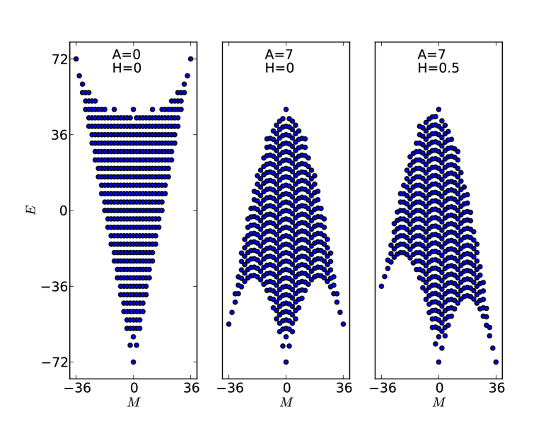
A configuration class is the subset of Ising configurations that have identical energy $E$ and magnetization $M$ (Lourenco 2012). The configuration classes for the $6\!\times\!6$ instance of Eq. (1) are shown in Fig. 1 for different values of $A$ and $H$. Changing the values of these parameters does not change the membership of the classes, but does affect the position of the classes in the $E$-$M$ plane. The pure antiferromagnet, $A\!=\!0$, is shown in the left-most panel, while the pure ferromagnetic Ising model is the reflection about the $x$-axis. At the critical field $H_{c}\!=\!4$, the right-edge of classes spanning the AFM configurations and the FM+ configuration are all degenerate at $E\!=\!-2N$ for the former. Such degeneracy never arises for the latter model, and this is one reason the AFM Ising model has more complicated behavior (Hwang 2007).

The effect of increasing $A$ is much different. The middle panel of Fig. 1 shows the arrangement of configuration classes for $A\!=\!7$, which is the value considered throughout this paper. The arrangement looks similar to the FM Ising model, with curved boundaries separating the classes locally minimizing $E$. For $A\!=\!8$ the AFM and FM classes are exactly degenerate. The right-most panel shows the effect of applying a field on the arrangement of the classes. Clearly, this shows that depending on the values of $A$ and $H$ the phase transition between the AFM and paramagnetic (PM) states can be either first order or second order.

Figure 2: Phase diagram for the mean-field Ising antiferromagnet with $A\!=\!7$ as determined by Metropolis Monte Carlo. The black curve with small circles at data points represents critical temperatures determined by extrapolation of cumulant crossings. The vertical ticks are spinodal points estimated from Monte Carlo scans in $H$; the horizontal size of the ticks indicate the uncertainty in the estimate. The points are connected with straight segments as a guide to the eye.

II Results

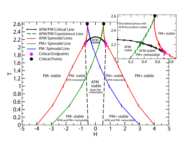
The phase diagram for $A\!=\!7$ deduced from Metropolis Monte Carlo (Metropolis 1953) simulation scans in $T$ and $H$ is shown in Fig. 2, along with the relevant spinodal lines. At $T\!=\!0$, first-order transitions between AFM and FM order occur at $|H|\!=\!0.5$. The distinction between FM configurations and PM configurations is rather arbitrary because there is not always a phase transition separating them. For $T\!>\!0$, coexistence curves for AFM/FM order are sketched approximately as dashed black lines. The curve of second-order AFM/PM phase transitions measured via the Binder cumulant method is shown as points connected by solid line segments. These extend to $H\!>\!0.5$, indicating slight reentrance of the AFM phase. Vertical ticks represent numerical determination of the spinodal lines (Miyashita 2008) including error estimates, with line segments included as guides to the eye. Below all the curves the AFM configurations are minima in the free energy: global minima and absolutely stable within the curves of the phase transitions, as opposed to metastable minima between the transition lines and the spinodals. The positively oriented PM$+$ configuration has a free-energy minimum to the right of the PM$+$ spinodal (green), while the negatively oriented PM$-$ configuration has a free energy minimum to the left of the PM$-$ spinodal line (blue).

Aside from the overall temperature scale, the features of the phase diagram considered so far are similar to those for a model in which the local AFM interaction term is replaced by the two-sublattice, mean-field approximation, i.e. the first term of Eq. (1) is replaced by $2|J|m_{\rm A}m_{\rm B}$ with $m_{A}$ and $m_{B}$ the individual sublattice magnetizations. In the mean-field approximation, the coexistence line joins the line of critical points at a tricritical point, from which the AFM and PM spinodal lines also emanate. However, the local nature of the AFM term in Eq. (1) admits fluctuations that significantly change the topology of the phase diagram at higher temperatures. Instead of merging at a tricritical point, the coexistence and second-order lines meet at an angle in a critical endpoint (Fisher 1990, Tsai 2007) at approximately $H\!=\!0.70$ and $T\!=\!2.09$, shown in the inset in Fig. 2. Above the temperature of the critical endpoint, the coexistence line continues to a critical point at approximately $H\!=\!0.561$ and $T\!=\!2.605$. The FM+ spinodal line also ends at this point. In the application of this model to spin-crossover materials, such a phase diagram provides for a variety of interesting hysteresis behaviors.

Figure 3: The free energy $E-TS$ calculated from the “two-dimensional” density of states, $g(E,M)$ for $A\!=\!7$ and $H\!=\!0.6$ for $T\!=\!2.15$, near the critical endpoint in the inset of Fig 2. The stable minimum is in the AFM region, but it is shallow and extends nearly to the PM+ region.

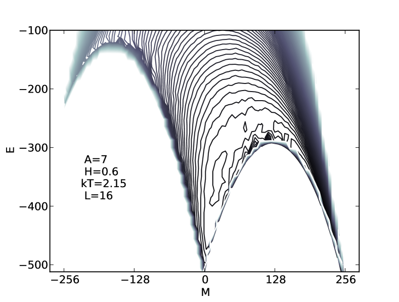
To understand the origin of these details, the Wang-Landau Monte Carlo method (Wang 2001) has been employed to estimate the density of states, $g(E,M)$. The entropy of the Hamiltonian is $S(E,M)\!=\!\ln{[g(E,M)]}$ and so the free energy is $F(E,M)=E-T\ln{\left[g\left(E,M\right)\right]}$ since all energies, including $T$, are in units of $|J|$. A contour plot of the free energy is shown in Fig. 3 for $L\!=\!16$, $A\!=\!7$, $H\!=\!0.6$, and $T\!=\!2.15$. These conditions are near the critical endpoint for this small system, but with the global minimum clearly associated with AFM configurations. As $H$ is increased this shallow minimum passes over to the region associated with FM/PM configurations. However, the phase diagram determined by the maximum in the specific heat from the Wang-Landau data (for this very small $L$) does not agree with the Metropolis data in several respects. The coexistence line of first order AFM/FM phase transitions rises vertically at $H\!=\!0.5$, before curving to the left for temperatures significantly above $T\!=\!1$ for $L\!\leq\!16$. No reentrant behavior has been observed in the Wang-Landau data. Instead, the maximum in the specific heat is observed to bifurcate at a field less than $H\!=\!0.5$. The left-most maximum corresponds the line of AFM/PM phase transitions, while the right-most maximum does not scale with the system size and possibly corresponds to a disorder line in the PM phase.

III Summary

Competition in the antiferromagnetic Ising model supplemented with a mean-field ferromagnetic term, leads to very rich thermodynamic behavior. One interesting feature is the transformation of a tricritical point (in the purely mean-field model) into a critical endpoint (in the full model). Preliminary results for Wang-Landau Monte Carlo on very small systems have not yet been harmonized with extensive results from Metropolis Monte Carlo calculations, particularly near the critical endpoint.

GB is supported by Oak Ridge National Laboratory, which is managed by UT-Battelle, LLC. PAR acknowledges hospitality at The University of Tokyo and partial support by NSF Grant No. DMR-1104829.

Fisher, M.E., Upton, P.J., 1990, Phys. Rev. Lett. 65, 2402.

Hwang, C.-O., Kim, S.-Y., Kang, D., Kim, J.M., 2007, J. Stat. Mech.: Theory and Experiment 2007, L05001.

Lourenco, B.J., Dickman, R., 2012, Int. J. Mod. Phys. C 23, 1240007.

Metropolis, N., Rosenbluth, A.W., Rosenbluth, M.N., Teller, A.H., Teller, E., 1953, J. Chem. Phys. 21, 1087.

Miyashita, S., Konishi, Y., Nishino, M., Tokoro, H., Rikvold, P.A., 2008, Phys. Rev. B 77, 014105.

Nakada, T., Rikvold, P.A., Mori, T., Nishino, M., Miyashita, S., 2011, Phys. Rev. B 84, 054433.

Nishino, M., Miyashita, S., 2013, Phys. Rev. B 88, 014108.

Tsai, S.-H., Wang, F., Landau, D.P., 2007, Phys. Rev. E 75, 061108.

Wang, F., Landau, D.P., 2001, Phys. Rev. Lett. 86, 2050; Phys. Rev. E 64, 056101.