Recursive families of higher order iterative maps

Abstract

To approximate a simple root of an equation we construct families of iterative maps of higher order of convergence. These maps are based on model functions which can be written as an inner product. The main family of maps discussed is defined recursively and is called Newton-barycentric. We illustrate the application of Newton-barycentric maps in two worked examples, one dealing with a typical least squares problem and the other showing how to locate simultaneously a great number of extrema of the Ackley’s function.

Key-words: Order of convergence, Newton’s method, Newton-Taylor map, Newton-barycentric map, least squares, Ackley’s function.

MSC2010: 49 M15, 65H05, 65H10.

1 Introduction

The classical Newton’s iterative scheme for approximating the roots of an equation has been generalized by many authors in order to define iterative maps going from cubical to arbitrary orders of convergence (see for instance [14], [10], [3], [7], [8], [12], [13], [15] and references therein). The primary aim of this work is to present a systematic construction of families of iterative maps of higher order of convergence.

All the iterative maps $t$ to be considered have a common structure $t(x)=x-\left[\phi(x)\right]^{-1}f(x)$, where $f$ is a real function with a simple zero at $z$. The function $\phi$ will be called a model function. This model function depends on $f$ and on another function $h$ which we name step function.

The families of iterative maps to be discussed are constructed by choosing distinct model functions $\phi$. We remark that our approach does not follow the traditional path for generating iterative maps by direct or inverse hyperosculatory interpolation (see, for instance [14]) or Taylor expansions around a zero of $f$ (see for instance [12]).

The paper is organized as follows. In Section 2 we introduce the notion of a model function $\phi$ and prove that the iterative map $t(x)=x-\left[\phi(x)\right]^{-1}f(x)$ has a certain order of convergence (see Proposition 2.1). The proof of Proposition 2.1 leads to the definition of a step function $h$. Then, taking distinct model functions we construct the so-called Taylor-type and barycentric-type maps. In both cases, the map $\phi$ can be written as the Euclidean inner product of two vectorial functions, one depending on $f$ and the other on the step function $h$. Such inner product enables us to prove that the iterative map $\phi$ is indeed a model function and the correspondent iterative map $t$ has a certain order of convergence (see propositions 2.2 and 2.3).

In the following section we construct recursively families of iterative maps $t_{j}$ with $j=0,1,\ldots,k$ (for a given positive integer $k$), called Newton-Taylor and Newton-barycentric. The respective step function $h_{j}$ (defined recursively) uses the classical Newton’s method as a starter. The model function in the Newton-Taylor family is of Taylor-type whereas for Newton-barycentric family is of barycentric type. The main result is Proposition 3.1 which shows that each member $t_{j}$ of the referred families has order of convergence at least $j+2$. We end Section 3 by briefly referring how to extend our iterative maps in order to deal with functions $f$ defined in $\mathbb{R}^{n}$.

The last section is devoted to the application of some Newton-barycentric formulas to concrete examples. The first example is a typical least squares problem. The other example shows the ability of these maps to locate simultaneously extrema of the Ackley’s function [1], a function widely used for testing optimization algorithms (see for instance [9]). This last numerical example shows that higher order iterative maps might be relevant in those real-world applications where it is important to get a simultaneous localization of a great number of extrema in $\mathbb{R}^{2}$, starting from a suitable set of data points in the domain of the objective function.

2 Iterative maps derived from model functions

Given a real-valued function $f$ defined on an open set $D\subset\mathbb{R}$, we assume that $f$ is sufficiently smooth in a neighborhood of a simple zero $z$ of $f$. In what follows we construct certain families of iterative maps $t$ generating a sequence $x_{k+1}=t(x_{k})$, $k=0,1,\ldots$, converging locally to $z$.

Let us first recall the notion of order of convergence of an iterative map $t$ (see for instance [14]). We say that $t$ has order order of convergence $p\geq 1$ if there exists a positive constant $c$, such that

$$\lim_{x\rightarrow z}\displaystyle{\frac{|z-t(x)|}{|z-x|^{p}}}=c.$$

It is well-known that an advantage of the superlinear convergence (that is, when $p>1$) is the assurance of the existence of a neighborhood of $z$ where the sequence $x_{k+1}=t(x_{k})$ converges to $z$ (see for instance [4]). However, in general, maps of higher order of convergence have expressions of increasing complexity, and so increasing its computational cost. This is one reason why among the families of iterative maps obtained in Section 3, the Newton-barycentric formulas are the ones used in the worked examples. These formulas are computationally more economic than the Newton-Taylor ones, which are only considered here as an illustration of our constructive process of generating iterative methods.

Proposition 2.1.

Let $z$ be a simple zero of a function $f:D\subset\mathbb{R}\mapsto\mathbb{R}$ and $\phi$ a sufficiently smooth function in a neighborhood of $z$, such that its derivatives $\phi^{(i)}$ satisfy the $j+1$ equalities

$$\begin{array}[]{l}\phi^{(i)}(z)=\displaystyle{\frac{f^{(i+1)}(z)}{i+1}},\qquad i=0,1,\ldots,j,\end{array}$$ (1)

for $j\geq 0$ a fixed integer. Then, for any initial value $x_{0}$ sufficiently close to $z$, the iterative process $x_{k+1}=t(x_{k})$, $k=0,1,\ldots$, with

$$t(x)=x-\phi^{-1}(x)\,f(x),$$ (2)

converges to $z$ and its order of convergence is at least $j+2$.

Proof.

From (2) it is obvious that the zero $z$ of $f$ is a fixed point of the map $t$ (that is, $t(z)=z$). Let us consider the function $\,\Delta t$ defined by

$$\Delta t(x)=t(x)-x.$$

Note that its derivatives are

$$\Delta^{(1)}t(x)=t^{(1)}(x)-1,\quad\mbox{and}\quad\Delta^{(i)}t(x)=t^{(i)}(x),\quad\mbox{for}\quad i\geq 2.$$

We now use induction on $j$ to prove that the hypotheses in (1) imply that $\Delta t(z)=0$, $\Delta^{(1)}t(z)=-1$, $\Delta^{(j)}t(z)=0$, for $j\geq 2$, and consequently $t$ has the referred order of convergence.

Let $j=0$. Rewriting (2) as

$$\phi(x)\,\Delta t(x)=-f(x),$$ (3)

and applying the derivative operator to this equation, we have

$$\phi^{(1)}(x)\,\Delta t(x)+\phi(x)\,\Delta^{(1)}t(x)=-f^{(1)}(x).$$ (4)

Since $\Delta t(z)=0$, and $\phi$ satisfies (1) with $i=0$, it follows that $f^{(1)}(z)\,\Delta^{(1)}(z)=-f^{(1)}(z).$ As $z$ is a simple zero for $f$, then

$$\Delta^{(1)}t(z)=-1\,\Longleftrightarrow\,t^{(1)}(z)=0,$$

which means that the iterative process generated by $t$ has local order of convergence $p$ at least $2$. That is, $p\geq j+2$.

Let $j=1$. Differentiating (4), we get

$$\phi^{(2)}(x)\,\Delta t(x)+2\,\phi^{(1)}(x)\,\Delta^{(1)}t(x)+\phi(x)\,\Delta^{(2)}t(x)=-f^{(2)}(x).$$

Since $\Delta t(z)=0$ and $\Delta^{(1)}t(z)=-1$, we obtain

$$-2\,\displaystyle{\frac{f^{(2)}(z)}{2}}+f^{(1)}(z)\,\Delta^{(2)}t(z)=-f^{(2)}(z).$$

Therefore $\Delta^{(2)}t(z)=t^{(2)}(z)=0$, and so the iterative process has local order of convergence at least $3=j+2$.

For an integer $m\geq 2$, assume that

$$\phi^{(j)}(z)=\displaystyle{\frac{f^{(j+1)}(z)}{j+1}},\quad\mbox{for}\quad j=0,1,\ldots,m,$$

and

$$\Delta^{(1)}t(z)=-1,\quad\Delta^{(j)}t(z)=0,\quad\mbox{for}\quad j=2,3,\ldots,m.$$ (5)

Let us show that $\Delta^{(m+1)}t(z)=t^{(m)}(z)=0$. From (3) and the Leibniz’s rule for the derivatives of the product, we have

$$\begin{array}[]{ll}&\phi^{(m+1)}(x)\,\Delta t(x)+\binom{m+1}{1}\phi^{(m)}(x)\,\Delta^{(1)}t(x)+\cdots+\binom{m+1}{m}\phi^{(1)}(x)\,\Delta^{(m)}t(x)+\\ &\hskip 56.9055pt+\phi^{(0)}(x)\,\Delta^{(m+1)}t(x)=-f^{(m+1)}(x).\end{array}$$

Thus, by the induction hypotheses, we obtain

$$-\binom{m+1}{1}\,\displaystyle{\frac{f^{(m+1)}(z)}{m+1}}+f^{(1)}(z)\,\Delta^{(m+1)}t(z)=-f^{(m+1)}(z)\,\Leftrightarrow\Delta^{(m+1)}t(z)=0.$$

Hence the iterative map $t_{m+1}$ has local order of convergence $p\geq m+2$ and the proof is complete. ∎

Remark 2.1.

The well-known result on the local order of convergence of the Newton’s map $t(x)=x-\left[f^{(1)}(x)\right]^{-1}f(x)$ follows immediately from Proposition 2.1. It is enough to see that (1) is verified for $j=0$, i.e. $\phi^{(0)}(z)=f^{(1)}(z)$, and so $t$ has local order of convergence at least 2.

A function like $\Delta t=t(x)-x$, satisfying the properties (5) in the proof of Proposition 2.1, will be called a step function and a function $\phi$ satisfying (1) will be called a model function.

Definition 2.1.

Let $z$ be a simple zero of a function $f:D\subset\mathbb{R}\mapsto\mathbb{R}$, $h$ and $\phi$ sufficiently smooth functions in a neighborhood of $z$, and $j\geq 0$ a fixed integer.

• A function $\phi$ is called a model function if it satisfies the $j+1$ conditions (1).

• A function $h$ is called a step function at $x=z$ (or simply a step function) if it satisfies the following $j+1$ equalities:

  $$\begin{array}[]{l}h(z)=0,\quad h^{(1)}(z)=-1\quad\mbox{and}\quad h^{(i)}(z)=0,\quad\mbox{for}\quad i=2,3,\ldots,j.\end{array}$$ (6)

2.1 The Taylor-type maps

As before we assume throughout that $z$ is a simple zero of a real function $f$. Let $k\geq 0$ be an integer. We now construct a family of iterative maps based on the following function

$$\phi_{k}(x)=f^{(1)}(x)+\displaystyle{\frac{f^{(2)}(x)}{2!}}\,h(x)+\displaystyle{\frac{f^{(3)}(x)}{3!}}\,h^{2}(x)+\cdots+\displaystyle{\frac{f^{(k+1)}(x)}{(k+1)!}}\,h^{k}(x),$$ (7)

where $h$ and $h^{k}$ denote respectively a given step function and its $k$-th power. In order to show that the iterative process generated by a map $t_{k}$, defined by

$$t_{k}(x)=x-\left[\phi_{k}(x)\right]^{-1}\,f(x),$$ (8)

has order of convergence at least $k+2$, we write $\phi_{k}$ as an inner product of two vectorial functions, one depending on $f$ and the other on the step function $h$. This simplifies considerably the necessary computations because of the orthogonality of a certain basis of $\mathbb{R}^{k+1}$ (see Lemma 2.1 below).

The function $\phi_{k}$ in (7) can be written as the following Euclidean inner product

$$\phi_{k}(x)=\langle U_{k}(x),V_{k}(x)\rangle,$$

with

$$V_{k}(x)=\left(1,h(x),h^{2}(x),h^{3}(x),\cdots,h^{k}(x)\right),$$ (9)

and

$$U_{k}(x)=\left(f^{(1)}(x),\frac{f^{(2)}(x)}{2!},\frac{f^{(3)}(x)}{3!},\ldots,\frac{f^{(k+1)}(x)}{(k+1)!}\right).$$

We now establish some properties of the function $V_{k}$ which are necessary to the proof of the Proposition 2.2 below.

Lemma 2.1.

Let $h$ be a step function at $x=z$ and $M_{k}$ the $(k+1)\times(k+1)$ matrix whose rows are the derivatives $V_{k}^{(0)}(z),V_{k}^{(1)}(z),\ldots,V_{k}^{(k)}(z)$ of $V_{k}$ in (9). Then, the set

$${\cal V}_{k}=\left\{V_{k}^{(0)}(z),V_{k}^{(1)}(z),\ldots,V_{k}^{(k)}(z)\right\},$$

is an orthogonal basis of $\mathbb{R}^{k+1}$. In particular, the matrix $M_{k}$ is diagonal and its rows are

$$\begin{array}[]{ll}V_{k}^{(0)}(z)&=(1,0,0,0,\cdots,0)\\ V_{k}^{(1)}(z)&=(0,-1,0,0,\cdots,0)\\ V_{k}^{(2)}(z)&=(0,0,2!,0,\cdots,0)\\ V_{k}^{(3)}(z)&=(0,0,0,-3!,\cdots,0)\\ &\vdots\\ V_{k}^{(k)}(z)&=(0,0,0,0,\cdots,(-1)^{k}\,k!).\end{array}$$ (10)

Proof.

Using the definition of step function, the $k$-fold differentiation of $V_{k}$ gives that each vector $V_{k}^{(i)}(z)$ has only a nonzero component which is the $(i+1)$-th one. In particular, this entry is $V^{(i)}_{k,i+1}(z)=(-1)^{i}\,i!$, for $i=0,1,\ldots,k$. Therefore, the set ${\cal V}_{k}$ is obviously orthogonal and $M_{k}$ is diagonal. ∎

Lemma 2.2.

For a positive integer $m$, the sum

$$s_{m}=1-\displaystyle{\frac{1}{2}}\binom{m}{1}+\displaystyle{\frac{1}{3}}\binom{m}{2}-\ldots+(-1)^{m}\,\displaystyle{\frac{1}{m+1}}\binom{m}{m}$$

is

$$s_{m}=\displaystyle{\frac{1}{m+1}}.$$

Proof.

The proof is straightforward by induction on $m$ and by well-known properties of the binomial coefficients. ∎

Proposition 2.2.

Let $f$ be a function satisfying the hypotheses of Proposition 2.1, $h$ a step function and $\phi_{k}$ given by (7). Then, $\phi_{k}$ is a model function and $t_{k}=x-\left[\phi_{k}(x)\right]^{-1}f(x)$ has local order of convergence at least $k+2$.

Proof.

Once we prove that $\phi_{k}$ is a model function the result that $t_{k}$ has local order of convergence at least $k+2$ follows from Proposition 2.1.

Let us use induction on $k$ to prove that $\phi_{k}$ is a function satisfying (1). For $k=1$, the function $\phi_{1}$ can be written as the inner product

$$\phi_{1}(x)=\langle U_{1}(x),V_{1}(x)\rangle,$$

with

$$\begin{array}[]{l}U_{1}(x)=\left(f^{(1)}(x),\displaystyle{\frac{f^{(2)}(x)}{2!}}\right)\quad\mbox{and}\quad V_{1}(x)=\left(1,h(x)\right).\end{array}$$

Since $h$ is a step function it satisfies $h(z)=0$ and $h^{(1)}(z)=-1$, and so

$$\phi_{1}(z)=\phi_{1}^{(0)}(z)=\langle U_{1}(z),V_{1}(z)\rangle=f^{(1)}(z).$$

Now, the first derivative of $\phi_{1}$ is

$$\phi_{1}^{(1)}(x)=\langle U_{1}^{(1)}(x),V_{1}^{(0)}(x)\rangle+\langle U_{1}^{(0)}(x),V_{1}^{(1)}(x)\rangle.$$

At $x=z$, we have

$$\begin{array}[]{l}U_{1}^{(0)}(z)=\left(f^{(1)}(z),f^{(2)}(z)/2\right),\qquad U_{1}^{(1)}(z)=\left(f^{(2)}(z),f^{(3)}(z)/2\right)\end{array}$$

and by Lemma 2.1, we obtain $V_{1}^{(0)}(z)=(1,0)$ and $V_{1}^{(1)}(z)=(0,-1)$. Then,

$$\phi_{1}^{(1)}(z) =\langle U_{1}^{(1)}(z),V_{1}^{(0)}(z)\rangle+\langle U_{1}^{(0)}(z),V_{1}^{(1)}(z)\rangle$$

$$=f^{(2)}(z)-\displaystyle{\frac{f^{(2)}(z)}{2}}=\displaystyle{\frac{f^{(2)}(z)}{2}}.$$

Thus, condition (1) holds for $k=1$.

For an integer $m\geq 2$, the induction basis is $h^{(1)}(z)=-1$, $h^{(i)}(z)=0$, with $i=0,2,\ldots,m$, and $\phi_{m}^{(0)}(z)=f^{(1)}(z)$, $\phi_{m}^{(1)}(z)=f^{(1)}(z)/2$, $\ldots$, $\phi_{m}^{(m-1)}(z)=f^{(m)}(z)/m$. As

$$\phi_{m}(x)=\langle U_{m}(x),V_{m}(x)\rangle,$$

the derivative of order $m$ of the inner product gives

$$\begin{array}[]{ll}\phi_{m}^{(m)}(x)&=<U_{m}^{(m)}(x),V_{m}^{(0)}(x)>+\binom{m}{1}\,<U_{m}^{(m-1)}(x),V_{m}^{(1)}(x)>+\\ \\ &\hskip 14.22636pt+\binom{m}{2}\,<U_{m}^{(m-2)}(x),V_{m}^{(2)}(x)>+\cdots+\binom{m}{m}\,<U_{m}^{(0)}(x),V_{m}^{(m)}(x)>.\end{array}$$ (11)

Let us prove that $\phi_{m}^{(m)}(z)=f^{(m+1)}(z)/(m+1)$. We have

$$\begin{array}[]{l}U_{m}^{(0)}(z)=\left(f^{(1)}(z),\,\displaystyle{\frac{f^{(2)}(z)}{2!}},\cdots,\displaystyle{\frac{f^{(m+1)}(z)}{(m+1)!}}\right)\\ U_{m}^{(1)}(z)=\left(f^{(2)}(z),\,\displaystyle{\frac{f^{(3)}(z)}{2!}},\cdots,\displaystyle{\frac{f^{(m+2)}(z)}{(m+1)!}}\right)\\ \hskip 56.9055pt\vdots\\ U_{m}^{(m)}(z)=\left(f^{(m+1)}(z),\,\displaystyle{\frac{f^{(m+2)}(z)}{2!}},\cdots,\displaystyle{\frac{f^{(2\,m+1)}(z)}{(m+1)!}}\right),\end{array}$$

and so by (10) the evaluation of (11) at $x=z$, gives

$$\begin{array}[]{ll}\phi_{m}^{(m)}(z)&=f^{(m+1)}(z)-\displaystyle{\frac{\binom{m}{1}}{2}}\,f^{(m+1)}(z)+\\ &\hskip 14.22636pt+\displaystyle{\frac{\binom{m}{2}}{3}}\,f^{(m+1)}(z)-\cdots+(-1)^{m}\displaystyle{\frac{\binom{m}{m}}{m+1}}\,f^{(m+1)}(z)=\displaystyle{\frac{f^{(m+1)}(z)}{m+1}},\end{array}$$

where the last equality follows from Lemma 2.2, which completes the proof. ∎

A function $\phi_{k}$ of the form (7) will be called a Taylor-type model function and the map $t_{k}$ given by (8) will be referred as a Taylor-type iterative map.

In paragraph 2.2 we will discuss another family of iterative maps which is computationally more interesting than Taylor-type ones in the sense it is deduced from a set of model functions $\phi_{k}$ which only uses the first derivative of the function $f$.

The first four Taylor-type maps are displayed in Table 1. Formulas similar to those in Table 1 have been attributed to Euler and Chebyshev (see Traub [14]).

$$\begin{array}[]{ | l | }\hline\cr t_{1}(x)=x-\displaystyle{\frac{2\,f(x)}{2\,f^{(1)}(x)+f^{(2)}(x)\,h(x)}}\\ t_{2}(x)=x-\displaystyle{\frac{6\,f(x)}{6\,f^{(1)}(x)+3f^{(2)}(x)\,h(x)+f^{(3)}(x)\,h^{2}(x)}}\\ t_{3}(x)=x-\displaystyle{\frac{24\,f(x)}{24\,f^{(1)}(x)+12f^{(2)}(x)\,h(x)+4\,f^{(3)}(x)\,h^{2}(x)+f^{(4)}(x)\,h^{3}(x)}}\\ t_{4}(x)=x-\displaystyle{\frac{120\,f(x)}{120\,f^{(1)}(x)+60f^{(2)}(x)\,h(x)+20\,f^{(3)}(x)\,h^{2}(x)+5\,f^{(4)}(x)\,h^{3}(x)+f^{(5)}(x)\,h^{4}(x)}}\\ \hline\cr\end{array}$$

Table 1: First four Taylor’s type maps.

2.2 The barycentric-type maps

The Taylor-type iterative maps $t_{k}$ were constructed using a model function $\phi_{k}$ defined as an inner product of two vectorial functions $U_{k}$ and $V_{k}$ depending respectively on the first $k$ derivatives of $f$ and on the powers of the step function $h$. We now consider another type of iterative maps $t_{k}$ by modifying the model function $\phi_{k}$ as follows: $\phi_{k}$ is the inner product of a constant vectorial function $U_{k}$ and a function $V_{k}$ depending only on the first derivative $f^{(1)}$ evaluated at $x+i\,h(x)$, for $i=0,\ldots,k$. Notably, we take

$$U_{k}(x)=\left(a_{0},a_{1},a_{2},\cdots,a_{k}\right)=\mathbf{a},$$ (12)

and

$$V_{k}(x)=\left(f^{(1)}(x),f^{(1)}(x+h(x)),\cdots,f^{(1)}(x+k\,h(x))\right),$$ (13)

where $h$ is a step function. If one proves that $\phi_{k}=\langle\mathbf{a},V_{k}(x)\rangle$ is a model function then, by Proposition 2.1, the respective process $t_{k}(x)=x-\left[\phi_{k}(x)\right]^{-1}f(x)$ has order of convergence at least $k+2$.

The next proposition shows that $\phi_{k}$ is a model function if and only if $U_{k}(x)=\mathbf{a}$ is the unique solution of a non homogeneous linear system. Moreover, this solution represents the barycentric coordinates of $\phi_{k}$ in a basis defined by the components of $V_{k}$.

Proposition 2.3.

Let $f$ be a function satisfying the hypotheses of Proposition 2.1, $h$ a step function, $k\geq 0$ a fixed integer and $\phi_{k}=\langle U_{k},V_{k}\rangle$, with $U_{k}$ and $V_{k}$ defined by (12) and (13). That is,

$$\phi_{k}(x)=a_{0}f^{(1)}(x)+a_{1}f^{(1)}(x+h(x))+\cdots+a_{k}f^{(1)}(x+k\,h(x)).$$ (14)

Then, the derivative of order $k$ of $V_{k}$, evaluated at $x=z$, is $V^{(k)}_{k}(z)=D_{k}\,R_{k}$, where $D_{k}$ and $R_{k}$ are the following $(k+1)\times(k+1)$ matrices

$$D_{k}=\operatorname{diag}\left(f^{(1)}(z),f^{(2)}(z),\cdots,f^{(k+1)}(z)\right),$$

and

$$R_{k}=\begin{bmatrix}1&1&1&1&\ldots&1\\ 1&0&-1&-2&\ldots&-(k-1)\\ 1&0&1&2^{2}&\ldots&(k-1)^{2}\\ \vdots&\vdots&\vdots&\vdots&\vdots&\vdots\\ 1&0&(-1)^{k}&(-1)^{k}2^{k}&\ldots&(-1)^{k}(k-1)^{k}\\ \end{bmatrix}.$$

Furthermore,

• The function $\phi_{k}$ is a model function if and only if

  $$U_{k}=\mathbf{a}=\left(a_{0},a_{1},a_{2},\cdots,a_{k}\right)$$

  is the (unique) solution of the linear system

  $$R_{k}\,\mathbf{a}=\mathbf{b},\quad\text{with}\quad\mathbf{b}=\left(1,1/2,1/3,\cdots,1/(k+1)\right).$$ (15)

  Also, this solution satisfies the equality

  $$\sum_{i=0}^{k}a_{i}=1.$$ (16)

• If $f^{(i)}(z)\neq 0$ for $i=1,\ldots,k$, then the function $U_{k}=\mathbf{a}$ represents the (normalized) barycentric coordinates of the model function $\phi_{k}$ relative to the basis,

  $${\cal V}_{k}=\left\{f^{(1)}(x),f^{(1)}(x+h(x)),\cdots,f^{(1)}(x+k\,h(x))\right\}.$$

Moreover, the iterative process generated by $t_{k}(x)=x-\left[\phi_{k}(x)\right]^{-1}f(x)$ has order of convergence at least $k+2$.

Proof.

For $i=0,1,\ldots,k$ the derivatives of order $i$ of $V_{k}$, evaluated at $x=z$, are:

$$V_{k}^{(0)} =f^{(1)}(z)\left(1,1,1,1,1,\cdots,1\right)$$

$$V_{k}^{(1)} =f^{(2)}(z)\left(1,0,-1,-2,-3,\cdots,-(k-1)\right)$$

$$V_{k}^{(2)} =f^{(3)}(z)\left(1,0,1,2^{2},3^{2},\cdots,(k-1)^{2}\right)$$

$$\vdots$$

$$V_{k}^{(k)} =f^{(k+1)}(z)\left(1,0,(-1)^{k},(-1)^{k}2^{k},(-1)^{k}3^{k},\cdots,(-1)^{k}(k-1)^{k}\right).$$

So, the equalities (15) hold.

For (i), since $\phi_{k}=\langle\mathbf{a},V_{k}(x)\rangle$, it is straightforward to verify that the conditions (1) for $\phi_{k}$ to be a model function are equivalent to the system $R_{k}\,\mathbf{a}=\mathbf{b}$. So, $U_{k}=\mathbf{a}$ must be a solution of this system. As $R_{k}$ is nonsingular, this is the unique solution. Furthermore, since $z$ is a simple zero of $f$, the equality (16) holds because it is just the first equation of the system $R_{k}\,\mathbf{a}=\mathbf{b}$.

For (ii), we need to show that for $\mathbf{\alpha}=(\alpha_{0},\alpha_{1},\ldots,\alpha_{k})\in\mathbb{R}^{k+1}$, such that

$$\alpha_{0}f^{(1)}(x)+\alpha_{1}f^{(1)}(x+h(x))+\ldots+\alpha_{k}f^{(k)}(x+k\,h(x))=\mathbf{0},$$ (17)

the only solution is $\mathbf{\alpha}=\mathbf{0}$. Differentiating (17) and evaluating at $x=z$, we obtain the homogeneous linear system

$$\operatorname{diag}\left(f^{(1)}(z),f^{(2)}(z),\cdots,f^{(k+1)}(z)\right)R_{k}\,\mathbf{\alpha}=\mathbf{0},$$

which admits only the solution $\mathbf{\alpha}=\mathbf{0}$ since both the diagonal matrix and $R_{k}$ are nonsingular.

The last assertion follows from Proposition 2.1 since by item (i) $\phi_{k}$ is a model function. ∎

The expressions for the first five barycentric maps are shown in Table 2.

$$\small\begin{array}[]{ | l | }\hline\cr t_{1}(x)=x-\displaystyle{\frac{2\,f(x)}{f^{(1)}(x)+f^{(1)}(x+h(x))}}\\ t_{2}(x)=x-\displaystyle{\frac{12\,f(x)}{5\,f^{(1)}(x)+8f^{(1)}(x+h(x))-f^{(1)}(x+2\,h(x))}}\\ t_{3}(x)=x-\displaystyle{\frac{24\,f(x)}{9\,f^{(1)}(x)+19f^{(1)}(x+h(x))-5\,f^{(1)}(x+2\,h(x))+f^{(1)}(x+3\,h(x))}}\\ t_{4}(x)=x-\displaystyle{\frac{720\,f(x)}{251\,f^{(1)}(x)+646f^{(1)}(x+h(x))-264\,f^{(1)}(x+2\,h(x))+106\,f^{(1)}(x+3h(x))-19f^{(1)}(x+4h(x))}}\\ t_{5}(x)=x-\displaystyle{\frac{1440\,f(x)}{\sum_{i=0}^{5}\alpha_{1}\,f^{(1)}(x+i\,h(x))}},\quad\mbox{with}\quad\alpha_{0}=475,\,\alpha_{1}=1427,\,\alpha_{2}=-798\\ \hskip 170.71652pt\begin{array}[]{l}\alpha_{3}=482,\,\alpha_{4}=-173,\,\alpha_{5}=27\\ \end{array}\\ \hline\cr\end{array}$$

Table 2: First five barycentric type maps.

3 Recursive families of iterative maps

We recall that a model function $\phi$ depends on a certain step function $h$. Now, for each model function $\phi_{j}$ entering in the definition of the map $t_{j}=x-\left[\phi_{j}(x)\right]^{-1}f(x)$, we use a step function which is defined recursively by $h_{j}(x)=t_{j-1}(x)-x$. The starter $t_{0}$ will be taken to be the Newton’s map $t_{0}(x)=x-[f^{(1)}(x)]^{-1}f(x)$. The next proposition shows that the iterative map $t_{m}$, defined recursively in (18), has local order of convergence $m+2$.

Proposition 3.1.

Let $z$ be a simple zero of a given function $f$ and $t_{0}$ the Newton’s map

$$t_{0}(x)=x-[f^{(1)}(x)]^{-1}f(x).$$

For a given natural number $m\geq 1$, define recursively the step function $h_{m}$ and the iterative map $t_{m}$ by

$$\begin{array}[]{l}h_{j}(x)=t_{j-1}(x)-x\\ \hskip 142.26378pt\quad j=1,2,\cdots,m\\ t_{j}(x)=x-\left[\phi_{j}(x)\right]^{-1}\,f(x),\end{array}$$ (18)

where $\phi_{j}$ is constructed using $h_{j}$ as step function and $\phi_{j}$ is either a Taylor-type or a barycentric-type map, respectively given by (7) and (14). Then, the map $t_{m}$ has local order of convergence at least $m+2$.

Proof.

It is only necessary to prove that each function $h_{j}$ is a step function and the statement follows from Propositions 2.2 and 2.3.

Let us apply induction on the integer $m$. For $m=1$, we have $h_{1}(x)=t_{0}(x)-x$ and so $h_{1}(z)=0$ and $h_{1}^{(1)}(z)=-1$. Let $m\geq 1$ be an integer. As $h_{m}^{(0)}(z)=0$, $h_{m}^{(1)}(z)=-1$ and for any integer $i$ such that $2\leq i\leq m$, we have $h_{m}^{(i)}(z)=0$, and so $h_{m}$ is a step function. ∎

We call Newton-Taylor and Newton-barycentric maps those maps $t_{k}$, defined in the Proposition 3.1, when one considers the model function to be respectively a Taylor-type map and a barycentrictype map. As before the name of these maps was chosen in order to emphasize that the starter step function is the Newton map.

Newton-Taylor maps

Let us compute the explicit expressions for the first two Newton-Taylor maps described in the previous proposition. The order of convergence of the first map $t_{1}$ and of the second map $t_{2}$ is respectively 3 and 4.

Order 3:

$$t_{1}(x)=x-\displaystyle{~\frac{2\,f(x)}{2\,f^{(1)}(x)+f^{(2)}(x)\,\left(\displaystyle{\frac{-f(x)}{f^{(1)}(x)}}\right)}}=x-\displaystyle{\frac{2\,f^{(1)}(x)\,f(x)}{2\left(f^{(1)}(x)\right)^{2}-f(x)\,f^{(2)}(x)}}.$$

The map $t_{1}$ coincides with the celebrated Halley’s method (see [6] and [14]).

Order 4:

$$t_{2}(x)=x-\displaystyle{\frac{6f(x)\,(f^{(1)}(x))^{2}}{f^{2}(x)\,f^{(3)}(x)+6\,(f^{(1)}(x))^{3}-3f(x)\,f^{(1)}(x)f^{(2)}(x)}.}$$

Newton-barycentric maps

Let us compute the explicit expressions of the first two Newton-barycentric maps $t_{1}$ and $t_{2}$. Recall that $t_{0}(x)=x-[f^{(1)}(x)]^{-1}\,f(x)$ and

$$h_{1}(x)=t_{0}(x)-x=-\frac{f(x)}{f^{(1)}(x)}.$$ (19)

Then

$$\phi_{1}(x)=a_{0}f^{(1)}(x)+a_{1}f^{(1)}\left(x+h_{1}(x)\right),$$

where $\mathbf{a}=(a_{0},a_{1})$ is the solution of the linear system (15) with $k=1$. This solution is $\mathbf{a}=(1/2,1/2)$ and so the Newton-barycentric map of order 3 is given by

Order 3:

$$t_{1}(x)=x-\displaystyle{\frac{2\,f(x)}{f^{(1)}(x)+f^{(1)}(x+h_{1}(x))}},$$ (20)

with $h_{1}$ is as in (19).

For the map of order 4, we have

$$\phi_{2}(x)=a_{0}f^{(1)}(x)+a_{1}f^{(1)}\left(x+h_{2}(x)\right)+a_{2}f^{(1)}\left(x+2h_{2}(x)\right),$$

with

$$h_{2}(x)=t_{1}(x)-x=\frac{-2f(x)}{f^{(1)}(x)+f^{(1)}\left(x+h_{1}(x)\right)},$$

and $\mathbf{a}=(a_{0},a_{1},a_{2})$ is the solution of the system (15) with $k=2$. This solution is $\mathbf{a}=\frac{1}{12}(5,8,-1)$, which gives

Order 4:

$$t_{2}(x)=x-\displaystyle{\frac{12\,f(x)}{5\,f^{(1)}(x)+8\,f^{(1)}\left(x-\frac{2\,f(x)}{f^{(1)}(x)+f^{(1)}(x+h_{1}(x))}\right)-f^{(1)}\left(x-\frac{4\,f(x)}{f^{(1)}(x)+f^{(1)}(x+h_{1}(x))}\right)}.}$$ (21)

The next three Newton-barycentric formulas are given in Table 2 where in each $t_{k}$ the step function $h$ should be substituted by $h_{k}$ given by (18).

Extension of the Newton-barycentric maps to $\mathbb{R}^{n}$

In the numerical examples presented in next section we apply Newton-barycentric maps to functions $f$ defined in $\mathbb{R}^{2}$. The following modifications were made in order to extend the Newton-barycentric maps to functions $f:\mathbb{R}^{2}\mapsto\mathbb{R}^{2}$.

The derivative $f^{(1)}$ is substituted by the Jacobian operator, that is $f^{(1)}(x)=\left[\partial f_{i}(x)/\partial x_{j}\right]_{i,j=1}^{n}$. Assuming that this matrix is nonsingular and taking $\Delta t_{k}(x)=t_{k}(x)-x$, the respective model function $\phi_{k}$ verifies

$$\phi_{k}(x)\,\Delta t_{k}(x)=-f(x).$$

Considering an initial guess $x^{(0)}\in\mathbb{R}^{n}$, each vector resulting from applying the map $t_{k}$ is computed by solving the linear system

$$\begin{array}[]{l}\phi_{k}(x^{(i)})\,\Delta t_{k}(x^{(i)})=-f(x^{(i)})\\ x^{(i+1)}=x^{(i)}+\Delta t_{k}(x^{(i)}),\quad i=0,1,\ldots.\end{array}$$ (22)

4 Numerical examples

In this section we apply the Newton-barycentric maps in two numerical examples. In Example 4.1 we locate a small number of extrema of a typical least squares problem and in Example 4.2 we locate a great number of local extrema of a function related to Ackley’s function (see [1]), using the scheme (22) with $i=0,1$.

In order to find the zeros of such functions let us start by detailing the procedure to be followed. For a given function $f$, defined in a rectangle $D=[x_{min},x_{max}]\times[y_{min},y_{max}]\subset\mathbb{R}^{2}$, we consider a rectangular grid in $D$ having mesh widths $d_{x}$ and $d_{y}$. We take for data points the vertices of the grid which are stored in a list ${\cal L}$.

We recall that an iterative map $t$ of order of convergence at least $2$ leads to a superlinear iterative process and so, for any initial point sufficiently close to a fixed point of $t$, the respective iterates either converge to the fixed point or go away from it. Therefore, given a $k\geq 0$, applying a Newton-barycentric map $t_{k}$ to each point in ${\cal L}$, the image points are either attracted to, or repelled from, the fixed points of $t_{k}$ eventually lying in $D$.

In order to test numerically some of the Newton-barycentric maps we only apply two iterations to the data points in the list ${\cal L}$. For this purpose, we consider $\epsilon$ to be a given tolerance and denote by $X^{(0)}$ an element of ${\cal L}$. The first and second iterates of a given map $t_{k}$ are denoted by $X^{(1)}$ and $X^{(2)}$ respectively. For each point $X^{(0)}$ in the list ${\cal L}$ we consider the following algorithm:

• If the Jacobian matrix $J_{f}(X^{(0)})$ is singular, the point $X^{(0)}$ is ignored and the next point in ${\cal L}$ is assigned to $X^{(0)}$.

• If both $X^{(1)}=t_{k}(X^{(0)})$ and $X^{(2)}=t_{k}(X^{(1)})$ do not belong to the domain $D$, the point $X^{(0)}$ is ignored and $X^{(0)}$ is taken to be the next point in ${\cal L}$ and proceed to step 1.

• If $||f(X^{(2)})||\leq\epsilon$ store $X^{(2)}$ in a list ${\cal C}$, otherwise let $X^{(0)}$ be the next point in ${\cal L}$ and go to step 1.

After testing all the elements in ${\cal L}$, if the list of the captured points ${\cal C}$ is not empty its elements will cluster near a fixed point of the iterative map $t_{k}$ in the search domain $D$. So, the plot of the captured points in ${\cal C}$ gives us a picture of the location of the fixed points of $t_{k}$. In fact, as it is well-known (see for instance [4]), for an iterative map of order $p\geq 2$, the error of an iterate $X^{(i)}$ is approximately $X^{(i+1)}-X^{(i)}$ and therefore it is expectable that the point $X^{(2)}$ will be closer to a fixed point of the map than $X^{(0)}$ and $X^{(1)}$.

Obviously we are not claiming that only two iterations of a higher order map are sufficient to locate all the simple zeros of a function $f$ in a domain $D$, by inspecting the list of the captured points ${\cal C}$. For a given tolerance $\epsilon$, one can only say that the captured points are likely to be close approximations of the zeros of $f$ eventually lying in $D$. In particular, for a discussion on the numerical validation of a few number of iterations of Newton’s method the reader is referred to [2], and for the fundamental question of proving the existence of zeros of nonlinear maps in $\mathbb{R}^{n}$ see for instance [5] and the references therein.

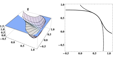
Figure 1: The “landscape” of the function $g$ (left) and the zero level curves of the components of $f$ given in the Example 4.1.

Example 4.1.

Consider the system

$$\left\{\begin{array}[]{l}x+y=1\\ x^{2}+y^{2}=0.8\\ x^{3}+y^{3}=0.68\\ x^{4}+y^{4}=0.01\\ \end{array}\right.$$

The first three equations were considered by Rutishauser [11] for illustrating a least squares problem. A least squares solution for the system can be found by minimizing the function

$$g(x,y)=s_{1}^{2}+s_{2}^{2}+s_{3}^{3}+s_{4}^{2},$$

where $s_{1}$ to $s_{4}$ are the residuals $s_{1}=x+y-1$, $s_{2}=x^{2}+y^{2}-0.8$, $s_{3}=x^{3}+y^{3}-0.68$, and $s_{4}=x^{4}+y^{4}-0.01$.

We apply some Newton-barycentric maps (see Table 2) in order to locate the roots of the equation $f(x,y)=\nabla g(x,y)=(0,0)$, where the components of the function $f=(f_{1},f_{2})$ are the following polynomials

$$\begin{array}[]{l}f_{1}(x,y)=2.-1.2\,x-4.08\,x^{2}+3.92\,x^{3}+6\,x^{5}+\\ \hskip 85.35826pt+8\,x^{7}+2\,y+4\,x\,y^{2}+6x^{2}\,y^{3}+8\,x^{3}\,y^{4},\\ \\ f_{2}(x,y)=-2.+2\,x-1.2\,y+4\,x^{2}\,y-4.08\,y^{2}+6\,x^{3}\,y^{2}+\\ \hskip 85.35826pt+3.92\,y^{3}+8\,x^{4}\,y^{3}+6\,y^{5}+8\,y^{7}.\end{array}$$

In Figure 1 we show both the plots of the of function $g$ “landscape” and the zero level curves of $f_{1}$ and $f_{2}$. Since $g$ has a flat “valley” and the zero level curves of $f$ seem to cross in several points it is not clear at all if a global minimum exists for this function in the following domain

$$D=[x_{min},x_{max}]\times[y_{min},y_{max}]=[-0.5,1.1]\times~[-0.7,1.1].$$ (23)

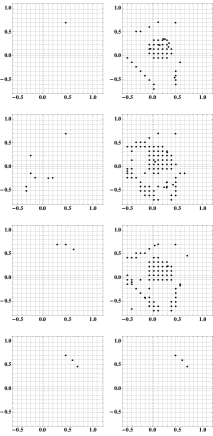
Figure 2: Captured points after two iterations of $t_{0}$, $t_{2}$, $t_{4}$, $t_{32}$ (left column) and $t_{1}$, $t_{3}$, $t_{5}$, $t_{43}$ (right column) – Example 4.1.

We consider a tolerance $\epsilon=0.001$ and a rectangular grid having mesh widths respectively $d_{x}\simeq 0.0876712$ and $d_{y}\simeq 0.0931507$. The respective list ${\cal L}$ contains the vertices of the mesh, that is $N=19\times 19=361$ data points, belonging to the search domain $D$. The previously described algorithm is applied to the data points using respectively the Newton-barycentric maps $t_{0}$ to $t_{5}$ and $t_{21},t_{32}$ (the map $t_{ij}$ is the composition $t_{i}(t_{j})$). The computations were carried out using the system Mathematica [16] in double precision.

The elements of the list of captured points (after two iterations of each map) are shown in Figure 2. The number of captured points is given in Table 3 and the captured points and their respective value by $g$ (rounded to $6$ decimal places) are in Table 4. From Figure 2, we see that the $18$ captured points cluster near 3 distinct points in the search domain $D$. It is clear from Table 4 that two global minimum have been located, one of them at $P=(0.459591,0.693716)$, with $g(P)=0.167974$.

$$\begin{array}[]{| c| c| c| c| c| c| c| c|c|}\hline\cr t_{i}&t_{0}&t_{1}&t_{2}&t_{3}&t_{4}&t_{5}&t_{21}&t_{32}\\ \hline\cr\verb+#+&1&50&8&89&4&77&6&18\\ \hline\cr\end{array}$$

Table 3: Number of captured points in the domain $D$ given in (23) – Example 4.1.

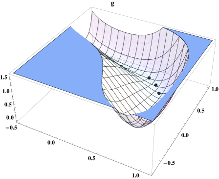
Figure 3: The three bold black points represent the clusters of captured points obtained after two iterations of $t_{32}$ – Example 4.1.

$$\begin{array}[]{| c | }\hline\cr(x_{i},y_{i},g(x_{i},y_{i}))\\ \hline\cr(0.459591,0.693716,0.167974)\\ \hline\cr(0.693716,0.459591,0.167974)\\ \hline\cr(0.593976,0.593976,0.169389)\\ \hline\cr\end{array}$$

Table 4: Three of the 18 points captured by $t_{32}$ (the other coincide up to 6 decimal places) with tolerance $\epsilon=0.001$– Example 4.1.

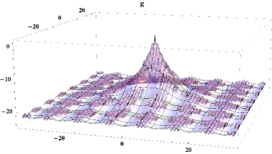
Figure 4: A 3D plot of the function $g$ given in (24).

Example 4.2.

In this example two iterations of Newton-barycentric maps are used in order to locate simultaneously a great number of zeros of a function $f$, related to the famous Ackley’s function [1]. We consider the following function

$$\begin{array}[]{l}g(x,y)=-(-20\,e^{s_{1}}-e^{s_{2}}+20+e),\quad\mbox{where}\\ \\ s_{1}=-0.2\sqrt{0.5\,(x^{2}+y^{2})}\quad\mbox{and}\quad s_{2}=0.5\left(\cos(2\pi\,x)+cos(2\pi\,y)\right).\end{array}$$ (24)

The function $g$ is the symmetric of the Ackley’s function which is widely used for testing optimization algorithms (see for instance [9]).

We consider the standard search domain $D=[x_{min},x_{max}]\times[y_{min},y_{max}]\subset\mathbb{R}^{2}$, with

$$x_{min}=y_{min}=-32.768\quad\mbox{ and}\quad x_{max}=y_{max}=32.768.$$

The “landscape” of $g$ is shown in Figure 4. At $(0,0)$ the function $g$ has a global maximum equal to zero and a great number of local extrema in $D$. Some extrema will be (simultaneously) located by applying two iterations of Newton-barycentric maps, namely (20), (21). For that purpose we consider $f:D\subset\mathbb{R}^{2}\mapsto\mathbb{R}^{2}$ to be the gradient of $g$ and we look for its zeros.

$$\begin{array}[]{| c| c| c| c|}\hline\cr x_{i}&y_{i}&f(x_{i},y_{i})&g(x_{i},y_{i})\\ \hline\cr-1.65185&-1.65185&(1.33227*10^{-15},1.33227*10^{-15})&-7.7843\\ \hline\cr-1.65185&1.65185&(1.33227*10^{-15},-1.33227*10^{-15})&-7.7843\\ \hline\cr-1.65185&-1.65185&(1.33227*10^{-15},1.33227*10^{-15})&-7.7843\\ \hline\cr-1.6103&0.&(-1.33227*10^{-15},0.)&-5.66925\\ \hline\cr-1.65185&1.65185&(1.33227*10^{-15},-1.33227*10^{-15})&-7.7843\\ \hline\cr 0.&-1.6103&(0.,-1.33227*10^{-15})&-5.66925\\ \hline\cr 0.&1.6103&(0.,1.33227*10^{-}{15})&-5.66925\\ \hline\cr 1.65185&-1.65185&(-1.33227*10^{-15},1.33227*10^{-}{15})&-7.7843\\ \hline\cr 1.6103&0.&(1.33227*10^{-15},0.)&-5.66925\\ \hline\cr 1.65185&1.65185&(-1.33227*10^{-15},-1.33227*10^{-15})&-7.7843\\ \hline\cr 1.65185&-1.65185&(-1.33227*10^{-15},1.33227*10^{-15})&-7.7843\\ \hline\cr 1.65185&1.65185&(-1.33227*10^{-15},-1.33227*10^{-15})&-7.7843\\ \hline\cr\end{array}$$

Table 5: Tolerance $\epsilon=0.1$ and a square mesh of width $d\simeq 1.6384$. Captured points by $t_{54}$ which are located at a distance not greater than 3 from the origin – Example 4.2.

The components of $f=\nabla g=(f_{1},f_{2})$ are

$$\begin{array}[]{ll}f_{1}(x,y)=&-\displaystyle{\frac{2.8284271247461907\times e^{-0.14142135623730953\,\sqrt{x^{2}+y^{2}}}\,x}{\sqrt{x^{2}+y^{2}}}}-\\ &\hskip 8.5359pt-3.141592653589793\times e^{0.5\,(\cos(2\,\pi\,x)+\cos(2\,\pi\,y))}\,\sin(2\pi\,x)=0\\ \\ f_{2}(x,y)&=-\displaystyle{\frac{2.8284271247461907\times e^{-0.14142135623730953\,\sqrt{x^{2}+y^{2}}}\,y}{\sqrt{x^{2}+y^{2}}}}-\\ &\hskip 8.5359pt-3.141592653589793\times e^{0.5\,(\cos(2\,\pi\,x)+\cos(2\,\pi\,y))}\,\sin(2\pi\,y)=0.\end{array}$$

The function $f$ is not defined at $x=y=0$, but can be continuously extended to the origin by taking $f(0,0)=(0,0)$. Moreover, the function is not differentiable at $(0,0)$ which explains why global search algorithms can hardly find the global extremum of $f$ located at the origin.

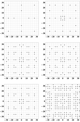
Figure 5: Tolerance $\epsilon=0.001$. Captured points after two iterations for $t_{0}$, $t_{2}$ and $t_{4}$ (left column), and $t_{1}$, $t_{3}$ and $t_{54}$ (right column) – Example 4.2.

$$\begin{array}[]{| c| c| c| c| c| c| c|}\hline\cr t_{i}&t_{0}&t_{1}&t_{2}&t_{3}&t_{4}&t_{54}\\ \hline\cr\verb+#+&12&28&60&64&52&208\\ \hline\cr\end{array}$$

Table 6: Number of captured points – Example 4.2.

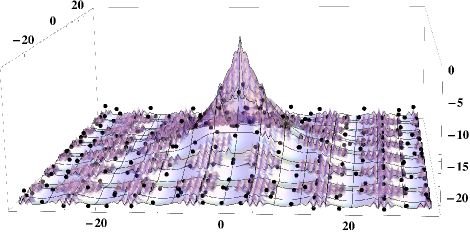
Figure 6: Tolerance $\epsilon=0.1$ and $d\simeq 1.6384$. The map $t_{54}$ captures $1458$ points after two iterations - Example 4.2.

For a tolerance $\epsilon=0.001$ we consider the set of $N=361$ points in $D$ formed by the vertices of a uniform large mesh of width $d=d_{x}=d_{y}\simeq 3.64089$. We apply two iterations of the Newton-barycentric maps $t_{0}$, $t_{1}$, $t_{2}$, $t_{3}$ and $t_{54}$ (the map $t_{54}$ is the composition $t_{5}\circ t_{4}$) to the data points following the algorithm previously described.

The captured points are shown in Figure 5 and the number of captured points is given in Table 6. The map $t_{54}$ is used just for comparison purposes with other Newton-barycentric maps of lower order. From Figure 5 it is reasonable to conclude that the zeros of $f$ are symmetrically located with respect to the axes. We remark that the Newton’s map $t_{0}$ only captures $9$ points after two iterations and in this sense the other higher order methods might give more insight on the location of the zeros of the function $f$ (or the extrema of Ackley’s function).

For the tolerance $\epsilon=0.1$ and $N=1681$ data points obtained from a mesh of width $d\simeq 1.6384$, the map $t_{54}$ is able to capture $664$ points $(x_{i},y_{i})$ clustering near the zeros of the function $f$. In Figure 6 we present the 3D plot of the captured points $(x_{i},y_{i},g(x_{i},y_{i}))$ for the function $g$ given in (24). In order to observe how close are the captured points by $t_{54}$ to the zeros of $f$, we give in Table 5 the coordinates of the points which are at a distance from $(0,0)$ not greater than $3$ as well as the respective values for $f$ and $g$.

References

- [1] D. H. Ackley, A connectionist machine for genetic hillclimbing. Kluwer, Boston, 1987.
- [2] G. Alefeld, A. Gienger and F. Potra, Efficient numerical validation of solutions of nonlinear systems, SIAM J. Numer. Anal., 31, 252-260, 1994.
- [3] L. Collatz, Functional Analysis and Numerical Mathematics. Academic Press, New York, 1966.
- [4] J. E. Dennis and J. J. Moré, A characterization of superlinear convergence and its application to quasi-Newton methods, Math. Comput., 28, 549-560, 1974.
- [5] A. Frommer, F. Hoxha and B. Lang, Proving the existence of zeros using the topological degree and interval arithmetic, J. Comput. Appl. Math., 199, 397-402, 2007.
- [6] E. Halley, A new exact and easy method for finding the roots of equations generally and without any previous reduction, Phil. Roy. Soc. London, 18, 1964, 136-147.
- [7] A. S. Householder, The Numerical Treatment of a Single Nonlinear Equation. McGraw-Hill, New York, 1970.
- [8] G. Labelle, On extensions of the Newton-Raphson iterative scheme to arbitrary orders Disc. Math Th. Comput Sc. (DMTCS), proc. AN, 2010, 845-856, Nancy, France.
- [9] J. J. Moré, B. S. Garbow and K. E. Hillstrom, Testing unconstrained optimization software, ACM Tras. Math. Soft., Vol. 7 (1), 17-41, 1981.
- [10] W. C. Rheinboldt, Methods for Solving Systems of Nonlinear Equations. 2nd Ed., SIAM, Philadelphia, 1998.
- [11] H. Rutishauser, Lectures on Numerical Mathematics. Birkhäuser, Boston, 1990.
- [12] P. Sebah and X. Gourdon, Newton’s method and high order iterations, 2001. Available from http://numbers.computation.free.fr/Constants/constants.html.
- [13] G. Fernández-Torres, Derivative free iterative methods with memory of arbitrary high convergence order, Numer. Alg., 2013, (pub. online Dec. 2013).
- [14] J. F. Traub, Iterative Methods for the Solution of Equations. Prentice-Hall, Englewood Cliffs, 1964.
- [15] S. Weerakoon, T. G. I. Fernando, A variant of Newton’s method with accelerated third-order convergence, App. Math. Lett., 13, 87-93, 2000.
- [16] S. Wolfram, The Mathematica Book. Wolfram Media, fifth ed., 2003.