Compressive Imaging via Approximate Message Passing with Image Denoising

Abstract

We consider compressive imaging problems, where images are reconstructed from a reduced number of linear measurements. Our objective is to improve over existing compressive imaging algorithms in terms of both reconstruction error and runtime. To pursue our objective, we propose compressive imaging algorithms that employ the approximate message passing (AMP) framework. AMP is an iterative signal reconstruction algorithm that performs scalar denoising at each iteration; in order for AMP to reconstruct the original input signal well, a good denoiser must be used. We apply two wavelet based image denoisers within AMP. The first denoiser is the “amplitude-scale-invariant Bayes estimator” (ABE), and the second is an adaptive Wiener filter; we call our AMP based algorithms for compressive imaging AMP-ABE and AMP-Wiener. Numerical results show that both AMP-ABE and AMP-Wiener significantly improve over the state of the art in terms of runtime. In terms of reconstruction quality, AMP-Wiener offers lower mean square error (MSE) than existing compressive imaging algorithms. In contrast, AMP-ABE has higher MSE, because ABE does not denoise as well as the adaptive Wiener filter.

I Introduction

I-A Motivation

Compressed sensing (CS) [1, 2] has sparked a tremendous amount of research activity in recent years, because it performs signal acquisition and processing using far fewer samples than required by the Nyquist rate. Breakthroughs in CS have the potential to greatly reduce the sampling rates in numerous signal processing applications such as cameras [3], medical scanners, fast analog to digital converters [4], and high speed radar [5].

Compressed sensing has been used in compressive imaging, where the input signal is an image, and the goal is to acquire the image using as few measurements as possible. Acquiring images in a compressive manner requires less sampling time than conventional imaging technologies. Applications of compressive imaging appear in medical imaging [6, 7, 8], seismic imaging [9], and hyperspectral imaging [10, 11].

I-B Related work

Many compressive imaging algorithms have been proposed in the literature. For example, Som and Schniter [12] modeled the structure of the wavelet coefficients by a hidden Markov tree (HMT), and applied a turbo scheme that alternates between inference on the HMT structure with standard belief propagation and inference on the compressed sensing measurement structure with the generalized approximate message passing algorithm. He and Carin [13] proposed a hierarchical Bayesian approach with Markov chain Monte Carlo (MCMC) for natural image reconstruction. Soni and Haupt [14] exploited a hierarchical dictionary learning method  [15] and assumed that projecting images onto the learned dictionary will yield tree-sparsity, and therefore the nonzero supports of the dictionary can be identified and estimated accurately by setting an appropriate threshold.

However, existing compressive imaging algorithms may either not achieve good reconstruction quality or not be fast enough. Therefore, in this paper, we focus on a variation of a fast and effective algorithm called approximate message passing (AMP) [16] to improve over the prior art. AMP is an iterative signal reconstruction algorithm that performs scalar denoising within each iteration, and proper selection of the denoising function used within AMP is needed to obtain better reconstruction quality. One challenge in applying image denoisers within AMP is that it may be hard to compute the so-called “Onsager reaction term” [17, 16] in the AMP iteration steps. The Onsager reaction term includes the derivative of the image denoising function, and thus if an image function does not have a convenient closed form, then the Onsager reaction term may be difficult to compute.

Dictionary learning is an effective technique that has attracted a great deal of attention in image denoising. Dictionary learning based methods [18, 19] generally achieve lower reconstruction error than wavelet-based methods. However, the learning procedure requires a large amount of training images, and may involve manual tuning. Owing to these limitations, our main focus in this paper is to integrate relatively simple and fast image denoisers into compressive imaging reconstruction algorithms.

Dabov et al. [20] developed an image denoising strategy that employs collaborative filtering in a sparse 3-D transform domain, and they offered an efficient implementation that achieves favorable denoising quality. Other efficient denoising schemes include wavelet-based methods. A typical wavelet-based image denoiser proceeds as follows: (i) apply a wavelet transform to the image and obtain wavelet coefficients; (ii) denoise the wavelet coefficients; and (iii) apply an inverse wavelet transform to the denoised wavelet coefficients, yielding a denoised image. Two popular examples of denoisers that can be applied to the wavelet coefficients are hard thresholding and soft thresholding [21]. Variations on the thresholding scheme can be found in [22, 23]; other wavelet-based methods were proposed by Simoncelli and Adelson [24], Mıhçak et al. [25], and Moulin and Liu [26].

I-C Contributions

The objective of this paper is to develop compressive imaging algorithms that are fast and reconstruct well. We apply the “amplitude-scale-invariant Bayes estimator” (ABE) [22] and the adaptive Wiener filter [25] as image denoisers within AMP. Our numerical results with these denoisers are promising, showing that our AMP based algorithms run at least 3.5 times faster than the prior art algorithms. Moreover, with a proper choice of image denoiser within AMP, the proposed algorithm also outperforms the prior art algorithms in reconstruction quality. Although we only test for two wavelet-based image denoisers within AMP, we believe that other image denoisers would also work within the AMP framework, and these denoisers need not be wavelet-based.

The remainder of the paper is arranged as follows. We review AMP in Section II, and describe the image denoisers [22, 25] that we use within AMP in Section III. Numerical results are presented in Section IV, and the paper concludes with a discussion in Section V.

II Review of Approximate Message Passing

II-A Problem setting

Before reviewing AMP, let us first model how measurements are obtained in a compressive imaging system.

Matrix channels: We rearrange the input image $\bf{x}$, which is comprised of $N$ pixels, as a column vector of length $N$ (for example, for a $512\times 512$ image, $N=512^{2}$). Then, we multiply $\bf{x}$ by a known measurement matrix ${\bf A}\in\mathbb{R}^{M\times N}$, which has $M$ rows (typically $M<N$). Finally, the measurements are corrupted by independent and identically distributed (i.i.d.) zero-mean Gaussian noise ${\bf z}$,

$$\mathbf{y=Ax+z}.$$ (1)

We observe the noisy vector $\mathbf{y}\in\mathbb{R}^{M}$, and want to estimate and reconstruct the original input signal $\mathbf{x}$ from $\mathbf{y}$ and $\mathbf{A}$.

Scalar channels: We now define scalar channels, and will describe in Section II-B how the matrix channel is converted to scalar channels in AMP. In scalar channels, the noisy observations obey

$$q_{i}=x_{i}+v_{i},$$ (2)

$i\in\{1,2,\ldots,N\}$, the subscript $(\cdot)_{i}$ denotes the $i$-th component of a vector (denoted by a lower case letter with bold font), and ${\bf x},{\bf q}\in\mathbb{R}^{N}$ are the input signal and the noisy observations, respectively. The noise ${\bf v}$ is i.i.d. Gaussian, $v_{i}\sim\mathcal{N}(0,\sigma^{2})$. Note that we use different notations for the noise and observations in matrix channels and scalar channels. The main difference between the two types of channels is that the observations ${\bf y}$ in the matrix channel contain linear combinations of the entries of ${\bf x}$.

II-B Algorithmic framework

We are now ready to describe AMP [16], which is an iterative signal reconstruction algorithm in matrix channels. Consider a matrix channel model (1) where the signal distribution follows ${x}_{i}\sim f_{X}$ and the noise is i.i.d. Gaussian. The entries of the measurement matrix ${\bf A}$ are i.i.d. $\mathcal{N}(0,\frac{1}{M})$ distributed, and thus the columns of the matrix have unit $\ell_{2}$-norm, on average. AMP [16] proceeds iteratively according to

$${\bf x}^{t+1} =\eta_{t}({\bf A}^{T}{\bf r}^{t}+{\bf x}^{t}),$$ (3)

$${\bf r}^{t} ={\bf y}-{\bf Ax}^{t}+\frac{1}{R}{\bf r}^{t-1}\langle\eta_{t-1}^{\prime}({\bf A}^{T}{\bf r}^{t-1}+{\bf x}^{t-1})\rangle,$$ (4)

where ${\bf A}^{T}$ is the transpose of ${\bf A}$, $R=M/N$ represents the measurement rate, $\eta_{t}(\cdot)$ is a denoising function at the $t$-th iteration, $\eta_{t}^{\prime}({\bf s})=\frac{\partial}{\partial{\bf s}}\eta_{t}({\bf s})$, and $\langle{\bf u}\rangle=\frac{1}{N}\sum_{i=1}^{N}u_{i}$ for some vector ${\bf u}=(u_{1},u_{2},\ldots,u_{N})$. The last term in equation (4) is called the “Onsager reaction term” [17, 16] in statistical physics. In the $t$-th iteration, we obtain the vectors ${\bf x}^{t}\in\mathbb{R}^{N}$ and ${\bf r}^{t}\in\mathbb{R}^{M}$. We highlight that the vector ${\bf A}^{T}{\bf r}^{t}+{\bf x}^{t}\in\mathbb{R}^{N}$ in (3) can be regarded as noisy measurements of ${\bf x}$ in the $t$-th iteration with noise variance $\sigma_{t}^{2}$, and therefore the denoising function $\eta_{t}(\cdot)$ is performed on a scalar channel (2). Let us denote the equivalent scalar channel at iteration $t$ by

$${\bf q}^{t}={\bf A}^{T}{\bf r}^{t}+{\bf x}^{t}={\bf x}+{\bf v}^{t},$$ (5)

where $v^{t}_{i}\sim\mathcal{N}(0,\sigma_{t}^{2})$. The asymptotic performance of AMP can be characterized by a state evolution (SE) formalism:

$$\sigma^{2}_{t+1}=\sigma^{2}_{z}+\frac{1}{R}E\left[\left(\eta_{t}\left(X+\sigma_{t}W\right)-X\right)^{2}\right],$$ (6)

where the random variables $W\sim\mathcal{N}(0,1)$ and $X\sim f_{X}$. Formal statements about SE appear in Bayati and Montanari [27]. Note that SE (6) tracks the noise variance for AMP iterations, but the noise variance $\sigma_{t+1}^{2}$ need not necessarily be the smallest possible, unless in each iteration the denoiser $\eta_{t}(\cdot)$ achieves the minimum mean square error (MMSE). We note in passing that we have proposed a denoiser called “MixD” [28] that achieves the MMSE of scalar channels (2), and thus applying MixD within AMP achieves the MMSE of matrix channels (1). On the other hand, it is unrealistic to expect existing image denoisers to achieve the MMSE, because the statistical distribution of natural images has yet to be determined. That said, running AMP with good image denoisers that achieve lower mean square error (MSE) may yield lower MSE in compressive imaging problems.

Finally, SE theoretically characterizes the noise variance $\sigma_{t}^{2}$ of the scalar channel at each iteration. However, the MSE performance of image denoisers cannot be characterized theoretically. Therefore, we must estimate the effective Gaussian noise level $\sigma^{2}_{t}$ empirically in each AMP iteration. The estimated noise variance $\widehat{\sigma}^{2}_{t}$ can be calculated as [29]:

$$\widehat{\sigma}^{2}_{t}=\frac{1}{M}\sum_{i=1}^{M}(r^{t}_{i})^{2},$$ (7)

where ${\bf r}^{t}$ is defined in (4).

III Image Denoising within AMP

In this section, we describe how wavelet-based image denoisers are applied within AMP, and then outline two image denoisers that were proposed by Figueiredo and Nowak [22] and Mıhçak et al. [25], respectively.

III-A Wavelet transforms in AMP

In image processing, one often computes the wavelet coefficients [30] of images, applies some signal processing technique to the wavelet coefficients, and finally applies the inverse wavelet transform to the processed coefficients to obtain processed images. We now show how image denoising can be performed within AMP in the wavelet domain. Let us denote the wavelet transform by $\mathcal{W}$ and the inverse wavelet transform by $\mathcal{W}^{-1}$. By applying the wavelet transform to a vectorized image signal ${\bf x}$ (a 2-dimensional wavelet transform is used), we obtain the wavelet coefficient vector ${\bf\theta_{x}}=\mathcal{W}{\bf x}$. Conversely, ${\bf x}=\mathcal{W}^{-1}{\bf\theta_{x}}$. Therefore, the matrix channel (1) becomes ${\bf y=A}\mathcal{W}^{-1}{\bf\theta_{x}+z}$, where ${\bf A}\mathcal{W}^{-1}$ can be regarded as a new matrix in the matrix channel (1) and ${\bf\theta_{x}}$ as the corresponding input signal.

Let us express the AMP iterations (3, 4) for settings where the matrix is ${\bf A}\mathcal{W}^{-1}$,

$$\theta^{t+1}_{\bf x} = \eta_{t}(({{\bf A}\mathcal{W}^{-1}})^{T}{\bf r}^{t}+\theta^{t}_{\bf x}),$$ (8)

$${\bf r}^{t} = {\bf y}-({\bf A}\mathcal{W}^{-1})\theta^{t}_{\bf x}$$ (9)

$$+\frac{1}{R}{\bf r}^{t-1}\langle\eta_{t-1}^{\prime}(({{\bf A}\mathcal{W}^{-1}})^{T}{\bf r}^{t-1}+\theta^{t-1}_{\bf x})\rangle$$

$$= {\bf y}-{\bf Ax}^{t}$$

$$+\frac{1}{R}{\bf r}^{t-1}\langle\eta_{t-1}^{\prime}(({{\bf A}\mathcal{W}^{-1}})^{T}{\bf r}^{t-1}+\theta^{t-1}_{\bf x})\rangle.$$

Because the wavelet transform matrix is orthonormal, i.e., $\mathcal{W}\mathcal{W}^{T}={\bf I}=\mathcal{W}\mathcal{W}^{-1}$, it can be shown that $({\bf A}\mathcal{W}^{-1})^{T}=\mathcal{W}{\bf A}^{T}$. Therefore, the input of the denoiser $\eta_{t}(\cdot)$ (8) becomes

$$({{\bf A}\mathcal{W}^{-1}})^{T}{\bf r}^{t}+\theta^{t}_{\bf x}=\mathcal{W}{\bf A}^{T}{\bf r}^{t}+\theta^{t}_{\bf x}=\mathcal{W}{\bf A}^{T}{\bf r}^{t}+\mathcal{W}{\bf x}^{t}=\mathcal{W}{\bf q}^{t},$$ (10)

where ${\bf q}^{t}$ (5) is the noisy image at iteration $t$, and $\mathcal{W}{\bf q}^{t}$ is the wavelet transform applied to the noisy image.

With the above analysis of the modified AMP (8, 9), we formulate a compressive imaging procedure as follows. Let us denote the the wavelet transform of the scalar channel (5) by

$$\theta_{\bf q}^{t}=\theta_{\bf x}+\theta_{\bf v}^{t},$$ (11)

where $\theta_{\bf q}^{t}=\mathcal{W}{\bf q}^{t}$, $\theta_{\bf x}=\mathcal{W}{\bf x}$, and $\theta_{\bf v}^{t}=\mathcal{W}{\bf v}^{t}$. First, ${\bf r}^{t}$ and ${\bf x}^{t}$ are initialized to all-zero vectors. Then, at iteration $t$ the algorithm proceeds as follows,

1. Calculate the residual term ${\bf r}^{t}$.

2. Calculate the noisy image ${\bf q}^{t}={\bf A}^{T}{\bf r}^{t}+{\bf x}^{t}$, and apply the wavelet transform $\mathcal{W}$ to the noisy image ${\bf q}^{t}$ to obtain wavelet coefficients $\theta_{\bf q}^{t}$, which are the inputs of the scalar denoiser $\eta_{t}(\cdot)$ in (8).

3. Apply the denoiser $\eta_{t}(\cdot)$ to the wavelet coefficients $\theta_{\bf q}^{t}$, and obtain denoised coefficients $\theta^{t+1}_{\bf x}$.

4. Apply the inverse wavelet transform $\mathcal{W}^{-1}$ to the coefficients $\theta_{\bf x}^{t+1}$ to obtain the estimated image ${\bf x}^{t+1}$, which is used to compute the residual term in the next iteration.

III-B Image denoisers

We choose to denoise the wavelet coefficients using scalar denoisers proposed by Figueiredo and Nowak [22] and Mıhçak et al. [25], respectively, because these two denoisers are simple to implement while revealing promising numerical results (see Section IV). We call the algorithm where ABE [22] is utilized within AMP “AMP-ABE,” and the algorithm where the adaptive Wiener filter [25] is utilized “AMP-Wiener.” In both algorithms, the variance of the noise $\sigma_{t}^{2}$ in the noisy image is obtained using (7). Because we use an orthonormal wavelet transform, the noise variance in the wavelet domain is equal to that in the image domain. Although we only show how to employ two image denoisers within AMP, they serve as a proof of concept that other image denoisers could also be applied within AMP, possibly leading to further improvements in both image reconstruction quality and runtime.

III-B1 Amplitude-scale-invariant Bayes estimator

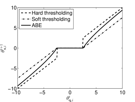
Figure 1: Comparison of ABE with hard and soft thresholding.

Figueiredo and Nowak’s denoiser [22] is an amplitude-scale-invariant Bayes estimator (ABE), and it is a scalar function. More specifically, for each noisy wavelet coefficient $\theta_{{\bf q},i}^{t}$ (11), the estimate of $\theta_{{\bf x},i}$ for the next iteration is

$${\theta}_{{\bf x},i}^{t+1}=\eta_{t}(\theta_{{\bf q},i}^{t})=\frac{\left((\theta_{{\bf q},i}^{t})^{2}-3\sigma_{t}^{2}\right)_{+}}{\theta_{{\bf q},i}^{t}},$$ (12)

where $\sigma_{t}^{2}$ is the noise variance of the scalar channel (5) at the $t$-th AMP iteration, and $(\cdot)_{+}$ is a function such that $(u)_{+}=u$ if $u>0$ and $(u)_{+}=0$ if $u\leq 0$. Note that because the wavelet transform matrix $\mathcal{W}$ is orthonormal, the variance of the noise ${\bf v}^{t}$ (5) is equal to the variance of $\theta_{\bf v}^{t}$ (11).

Figure 1 illustrates the ABE function. It can be seen that ABE offers a compromise between the hard thresholding, i.e., $\eta(u,\tau)=u\cdot\mathbbm{1}_{(u>|\tau|)}$, where $\mathbbm{1}_{\{\cdot\}}$ denotes an indicator function, and soft thresholding, i.e., $\eta(u,\tau)=\text{sign}(u)\cdot(|u|-\tau)_{+}$, proposed by Donoho and Johnstone [21]. ABE is convenient to utilize, because there is no need to tune the thresholding values, and ABE has been shown to outperform both hard and soft thresholding methods for image denoising [22].

The ABE function is continuous and differentiable except for two points ($\theta_{{\bf q},i}^{t}=\pm\sqrt{3}\sigma_{t}$), and we calculate the derivative of this denoising function numerically to obtain the Onsager reaction term in (4).

III-B2 Adaptive Wiener filter

Mıhçak et al. [25] proposed a method to estimate the variances of the wavelet coefficients, and then apply the corresponding Wiener filter to each wavelet coefficient. The variance of the noisy wavelet coefficient $\theta_{{\bf q},i}^{t}$ is estimated from its neighboring coefficients. More specifically, a set of $3\times 3$ or $5\times 5$ neighboring coefficients $\mathcal{N}_{i}$ that is centered at $\theta_{{\bf q},i}^{t}$ is considered, and the variance of $\theta_{{\bf q},i}^{t}$ is estimated by averaging the sum of $(\theta_{{\bf q},k}^{t})^{2}$ where $k\in\mathcal{N}_{i}$. This method of averaging the neighboring coefficients can be regarded as first convolving a $3\times 3$ or $5\times 5$ mask of all $1$’s with the matrix of squared wavelet coefficients $\theta_{\bf q}^{t}$, and then dividing by the normalizing constant $9$ (for a $3\times 3$ mask) or $25$ (for a $5\times 5$ mask). Other masks can be applied to produce different and possibly better denoising results. For example, we have found that the mask

$$\begin{matrix}&1&1&1&\\ 1&1&2&1&1\\ 1&2&3&2&1\\ 1&1&2&1&1\\ &1&1&1&\end{matrix}$$

obtains lower MSE than other $5\times 5$ masks we have considered. Recall the scalar channel defined in (11) where the noise variance is ${\sigma}_{t}^{2}$; we estimate the variance of a noisy wavelet coefficient $\theta_{{\bf q},i}^{t}$ by $\widehat{\sigma}_{i}^{2}$, and the variance of the true wavelet coefficient $\theta_{{\bf x},i}^{t}$ by $\widehat{\sigma}_{i}^{2}-\sigma_{t}^{2}$. Therefore, the scaling factor in the Wiener filter [32] is given by $\frac{\widehat{\sigma}_{i}^{2}-\sigma_{t}^{2}}{(\widehat{\sigma}_{i}^{2}-\sigma_{t}^{2})+\sigma_{t}^{2}}$, and the adaptive Wiener filter being used as the denoising function can be expressed as follows,

$${\theta}_{{\bf x},i}^{t+1}=\eta_{t}(\theta_{{\bf q},i}^{t})=\frac{\widehat{\sigma}_{i}^{2}-\sigma_{t}^{2}}{(\widehat{\sigma}_{i}^{2}-\sigma_{t}^{2})+\sigma_{t}^{2}}\theta_{{\bf q},i}^{t}=\frac{\widehat{\sigma}_{i}^{2}-\sigma_{t}^{2}}{\widehat{\sigma}_{i}^{2}}\theta_{{\bf q},i}^{t}.$$ (13)

Finally, the derivative of this denoising function with respect to $\theta_{{\bf q},i}^{t}$ is simply the scaling factor $\frac{\widehat{\sigma}_{i}^{2}-\sigma_{t}^{2}}{\widehat{\sigma}_{i}^{2}}$ of the Wiener filter, and so the Onsager reaction term in (4) can be obtained efficiently.

In standard AMP [16], the denoising function $\eta_{t}(\cdot)$ is separable, meaning that ${\theta}_{{\bf x},i}^{t+1}$ only depends on its corresponding noisy wavelet coefficient ${\theta}_{{\bf q},i}^{t}$. In the adaptive Wiener filter, however, the estimated variance $\widehat{\sigma}_{i}^{2}$ of each noisy wavelet coefficient depends on the neighboring coefficients of ${\theta}_{{\bf q},i}^{t}$, and so the denoising function in (13) implicitly depends on the neighboring coefficients of ${\theta}_{{\bf q},i}^{t}$. Therefore, the adaptive Wiener filter in (13) is not a strictly separable denoising function, and AMP-Wiener encounters convergence issues. Fortunately, a technique called “damping” [33] solves for the convergence problem of AMP-Wiener. Specifically, damping is an extra step in the AMP iteration (3); instead of updating the value of ${\bf x}^{t+1}$ by the output of the denoiser $\eta_{t}({\bf A}^{T}{\bf r}^{t}+{\bf x}^{t})$, we assign a weighted sum of $\eta_{t}({\bf A}^{T}{\bf r}^{t}+{\bf x}^{t})$ and ${\bf x}^{t}$ to ${\bf x}^{t+1}$ as follows,

$${\bf x}^{t+1}=(1-\lambda)\cdot\eta_{t}({\bf A}^{T}{\bf r}^{t}+{\bf x}^{t})+\lambda\cdot{\bf x}^{t},$$ (14)

for some constant $0\leq\lambda<1$. It has been shown by Rangan et al. [33] that sufficient damping ensures the convergence of AMP where the measurement matrix ${\bf A}$ is not i.i.d. Gaussian. However, we did indeed use i.i.d. Gaussian matrices in our numerical results in Section IV, and damping solved the convergence problem of AMP-Wiener, which suggests that damping may be an effective technique when various convergence issues arise in AMP based algorithms. We note in passing that other techniques such as SwAMP [34] and ADMM-GAMP [35] also solve for the convergence problem in AMP.

IV Numerical Results

Having described the AMP algorithm [16] and two image denoisers [22, 25], in this section we present the numerical results of applying these two denoisers within AMP.

IV-A Reconstruction quality and runtime

We compare AMP-ABE and AMP-Wiener with three prior art compressive imaging algorithms, (i) Turbo-BG proposed by Som and Schniter [12]; (ii) Turbo-GM, also by Som and Schniter [12]; and (iii) a Markov chain Monte Carlo (MCMC) method by He and Carin [13]. Both Turbo-BG and Turbo-GM are also message passing based algorithms. However, these two algorithms require more computation than AMP-ABE and AMP-Wiener, because they include two message passing procedures; the first procedure solves for dependencies between the wavelet coefficients and the second procedure is AMP. The performance metrics that we use to compare the algorithms are runtime and normalized MSE (NMSE), $\text{NMSE}({\bf x},\widehat{\bf x})=10\log_{10}(\|{\bf x-\widehat{x}}\|_{2}^{2}/\|{\bf x}\|_{2}^{2})$, where $\widehat{\bf x}$ is the estimate of the vectorized input image ${\bf x}$. In all simulations, we use the Haar wavelet transform [30].

Let us begin by contrasting the three prior art compressive imaging algorithms based on the numerical results provided in [12]. Turbo-BG and Turbo-GM have similar runtimes; the NMSE of Turbo-GM is typically 0.5 dB better (lower) than the NMSE of Turbo-BG. At the same time, the NMSE of the MCMC algorithm [13] is comparable to those of Turbo-BG and Turbo-GM, but MCMC is 30 times slower than the Turbo approaches of Som and Schniter [12]. Other algorithms have also been considered for compressive imaging. For example, compressive sampling matching pursuit (CoSaMP) [36] requires only half the runtime of Turbo-GM, but its NMSE is roughly 4 dB worse than that of Turbo-GM; and model based CS [37] is twice slower than Turbo-GM and its NMSE is also roughly 4 dB worse. Therefore, we provide numerical results for Turbo-BG, Turbo-GM, MCMC, and our two proposed AMP based approaches.

Numerical setting: We downloaded 591 images from “pixel-wise labeled image database v2” at http://research. microsoft.com/en-us/projects/objectclassrecognition, and extracted image patches using the following two methods.

• Method 1: A $192\times 192$ patch is extracted from the upper left corner of each image, and then the patch is resized to $128\times 128$; this image patch extraction method was used by Som and Schniter [12].

• Method 2: A $192\times 192$ patch is extracted from the upper left corner of each image without resizing.

The measurement matrix ${\bf A}\in\mathbb{R}^{M\times N}$ is generated with i.i.d. Gaussian entries distributed as $\mathcal{N}(0,\frac{1}{M})$; each column is then normalized to have unit norm. For $128\times 128$ patches extracted by Method 1, the number of measurements $M=5,000$, which is identical to the numerical setting by Som and Schniter [12]. For $192\times 192$ patches extracted by Method 2, the number of measurements $M=11,059$, i.e., the measurement rate is $0.3$. In both methods, the measurements ${\bf y}$ are noiseless, i.e., ${\bf y=Ax}$. Finally, we set the number of AMP iterations to be 30 and the damping constant $\lambda$ (14) for AMP-Wiener to be $0.1$.

Algorithm	NMSE (dB)	Runtime (sec)
Turbo-BG [12]	-20.37	12.39
Turbo-GM [12]	-20.72	12.47
MCMC [13]	-20.31	423.15
AMP-ABE	-19.30	3.39
AMP-Wiener	-21.00	3.34

TABLE I: NMSE and runtime averaged over 591 image patches: a $192\times 192$ patch from the upper left corner of each image is first extracted, and then resized to $128\times 128$. The number of measurements $M=5,000$, and the measurements are noiseless.

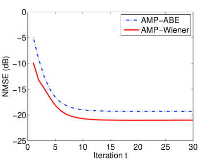
Figure 2: Average NMSE over 591 images from AMP iteration 1 to iteration 30. Image patches are extracted by Method 1: a $192\times 192$ patch from the upper left corner of each image is first extracted, and then resized to $128\times 128$.

Result 1: Tables I and II show the NMSE and runtime averaged over the 591 image patches that are extracted by Methods 1 and 2, respectively. Runtime is measured in seconds on a Dell OPTIPLEX 9010 running an Intel(R) $\text{Core}^{\text{TM}}$ i7-860 with 16GB RAM, and the environment is Matlab R2013a. Figures 2 and 3 complement Tables I and II, respectively, by plotting the average NMSE over 591 images from iteration 1 to iteration 30.

It can be seen from Table I that the NMSE of AMP-Wiener is the best (lowest) among all the algorithms compared. At the same time, AMP-Wiener runs approximately 3.5 times faster than the Turbo approaches of Som and Schniter [12], and 120 times faster than MCMC [13]. Although AMP-ABE does not outperform the competing algorithms in terms of NMSE, it runs as fast as AMP-Wiener.

Table I presents the runtimes of AMP-ABE and AMP-Wiener for image patches extracted by Method 1 with 30 iterations. However, we can see from Figure 2 that AMP-ABE and AMP-Wiener with fewer iterations already achieve NMSEs that are close to the NMSE shown in Table I. In Figure 2, the horizontal axis represents iteration numbers, and the vertical axis represents NMSE. It is shown in Figure 2 that the NMSE drops markedly from $-10$ dB to $-21$ dB for AMP-Wiener (solid line) and from $-5$ dB to $-19$ dB for AMP-ABE (dash-dot line), respectively. Note that the average NMSE is approximately $-21$ dB for AMP-Wiener and $-19$ dB for AMP-ABE around iteration 15. Therefore, we may halve the runtimes of AMP-ABE and AMP-Wiener (to approximately 1.7 seconds) by reducing the number of AMP iterations from 30 to 15.

The simulation for the larger image patches extracted by Method 2 is slow, and thus the results for Turbo-BG and MCMC have not been obtained for Table II. We believe that Turbo-BG is only slightly worse than Turbo-GM. At the same time, we did test for MCMC on several images, and found that the NMSEs obtained by MCMC were usually 0.5 dB higher than AMP-Wiener and the runtimes of MCMC usually exceeded 1,500 seconds. Similar to Figure 2, it can be seen from Figure 3 that the runtimes of our AMP based approaches could be further reduced by reducing the number of AMP iterations without much deterioration in estimation quality.

Algorithm	NMSE (dB)	Runtime (sec)
Turbo-GM [12]	-19.64	56.12
AMP-ABE	-17.57	15.99
AMP-Wiener	-20.29	15.53

TABLE II: NMSE and runtime averaged over 591 images extracted by Method 2: a $192\times 192$ patch is extracted from the upper left corner of each image. The number of measurements $M=11,059$, and the measurements are noiseless.

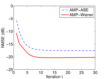
Figure 3: Average NMSE over 591 images from AMP iteration 1 to iteration 30. Image patches are extracted by Method 2: a $192\times 192$ patch is extracted from the upper left corner of each image.

Result 2: As a specific example, Figure 4 illustrates one of the 591 image patches and the estimated patches using AMP-Wiener at iterations 1, 3, 7, 15, and 30. We also present the estimated patches using Turbo-GM and MCMC. It can be seen from Figure 4 that the estimated images using AMP-Wiener are gradually denoised as the number of iterations is increased, and the NMSE achieved by AMP-Wiener at iteration 15 already produces better reconstruction quality than Turbo-GM and MCMC.

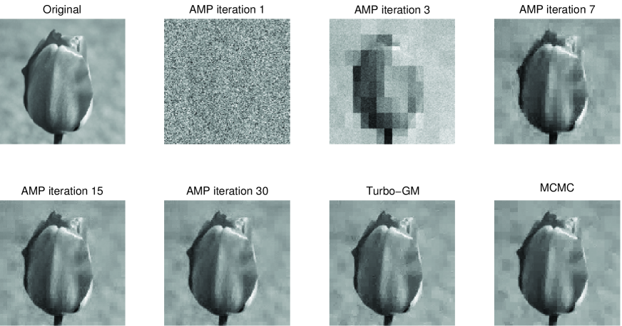
Figure 4: Original “10_5_s.bmp” input image, the estimated images using AMP-Wiener at iterations 1, 3, 7, 15, 30, and the estimated images using Turbo-GM and MCMC. The image patch is extracted by Method 1: a $192\times 192$ patch is first extracted, and then resized to $128\times 128$. The NMSE of each estimated image is as follows, AMP-Wiener iteration 1, $-11.46$ dB; AMP-Wiener iteration 3, $-18.17$ dB; AMP-Wiener iteration 7, $-26.28$ dB; AMP-Wiener iteration 15, $-30.07$ dB; AMP-Wiener iteration 30, $-30.36$ dB; Turbo-GM [12], $-29.62$ dB; MCMC [13], $-29.13$ dB.

IV-B Performance of scalar denoisers

Having seen that AMP-Wiener consistently outperforms AMP-ABE, let us now understand why AMP-Wiener achieves lower NMSE than AMP-ABE.

We test for ABE [22] and the adaptive Wiener filter [25] as scalar image denoisers in scalar channels as defined in (2). In this simulation, we use the 591 image patches extracted by Method 2, and add i.i.d. Gaussian noise $\mathcal{N}(0,\sigma^{2})$ to the image patches. The pixel values are normalized to be between $0$ and $1$, and we verified from the simulations for Table II that the estimated noise variances of the scalar channels in AMP iterations are typically between $1\times 10^{-4}$ and $1$. In Figure 5, the vertical axis represents NMSE, and the horizontal axis represents different noise variances varying from $1\times 10^{-4}$ to $1$ . It is shown in Figure 5 that the adaptive Wiener filter (solid line) consistently achieves lower NMSE than ABE (dash-dot line) for all noise variances, which suggests that AMP-Wiener outperforms AMP-ABE in every AMP iteration, and thus outperforms AMP-ABE when we stop iterating in iteration 30. Therefore, in order to achieve favorable reconstruction quality, it is important to select a good image denoiser within AMP. With this in mind, we include the NMSE of the image denoiser “block-matching and 3-D filtering” BM3D [20] in Figure 5, and find that BM3D (dashed line) has lower NMSE than the adaptive Wiener filter, especially when the noise variance is large. Note that the NMSEs of ABE for difference noise variances are within 1 dB of the NMSEs of the adaptive Wiener filter, but this performance gap in scalar denoisers is amplified to more than 2 dB (refer to Table II) when applying the scalar denoisers within AMP. In other words, it is possible that applying BM3D within AMP could achieve better reconstruction quality than AMP-Wiener. However, one challenge of applying BM3D within AMP will be that it is not clear whether the Onsager reaction term in (4) can be computed in closed form or numerically, and thus an alternative way of approximating the Onsager reaction term may need to be developed. During the review process of our paper, Metzler et al. [38] showed how to compute the Onsager correction term numerically, thus allowing to use different image denoisers within AMP.

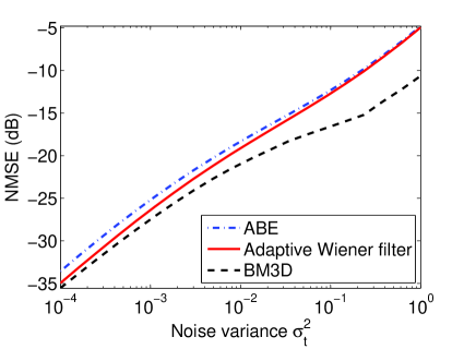
Figure 5: Average NMSE over 591 images versus noise variance. Image patches are extracted by Method 2: a $192\times 192$ patch is extracted from the upper left corner of each image. These image denoisers are applied to scalar channels (2).

IV-C Reconstruction quality versus measurement rate

Finally, we also evaluate the performance of each algorithm by plotting the NMSE (average NMSE over 591 images) versus the measurement rate $R=M/N$. The measurement matrix ${\bf A}$ is generated the same way as the numerical setting in Section IV-A.

Result: Figures 6 and 7 illustrate how the NMSEs achieved by AMP-Wiener and Turbo-GM vary when the measurement rate $R$ changes, where the horizontal axis represents the measurement rate $R=M/N$, and the vertical axis represents NMSE. Figures 6 shows the results for image patches extracted by Method 1, and the measurement rate $R$ varies from $0.1$ to $1$. Figure 7 shows the results for image patches extracted by Method 2. Because the simulation for $192\times 192$ image patches is relatively slow, we only show results for $R$ that varies from $0.1$ to $0.6$. It can be seen from Figures 6 and 7 that AMP-Wiener (solid line with pentagram markers) achieves lower NMSE than that of Turbo-GM (dash-dot line with asterisks) for all values of $R$.

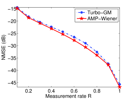
Figure 6: Average NMSE over 591 images versus measurement rate. Image patches are extracted by Method 1: a $192\times 192$ patch from the upper left corner of each image is first extracted, and then resized to $128\times 128$.

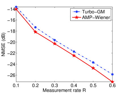
Figure 7: Average NMSE over 591 images versus measurement rate. Image patches are extracted by Method 2: a $192\times 192$ patch is extracted from the upper left corner of each image.

V Discussion

In this paper, we proposed compressive imaging algorithms that apply image denoisers within AMP. Specifically, we used the “amplitude-scale-invariant Bayes estimator” (ABE) [22] and an adaptive Wiener filter [25] within AMP. Numerical results showed that AMP-Wiener achieves the lowest reconstruction error among all competing algorithms in all simulation settings, while AMP-ABE also offers competitive performance. Moreover, the runtimes of AMP-ABE and AMP-Wiener are significantly lower than those of MCMC [13] and the Turbo approaches [12], and Figures 2 and 3 suggest that the runtimes of our AMP based algorithms could be reduced further if we accept a slight deterioration in NMSE.

Recall that the input of the denoising function $\eta_{t}$ in (3) is a noisy image with i.i.d. Gaussian noise, and so we believe that any image denoiser that deals with i.i.d. Gaussian noise can be applied within AMP. At the same time, in order to develop fast AMP based compressive imaging algorithms, the image denoisers that are applied within AMP should be fast. By comparing the denoising quality of ABE [22] and the adaptive Wiener filter [25] as image denoisers in scalar channels, we have seen that AMP with a better denoiser produces better reconstruction quality for compressive imaging problems. With this in mind, employing more advanced image denoisers within AMP may produce promising results for compressive imaging problems. The development of such compressive imaging algorithms is left for future work.

This paper used squared error ($\ell_{2}$-norm error) as the performance metric, and AMP-Wiener was shown to outperform the prior art. Besides the $\ell_{2}$-norm error, Bayati and Montanari [27] have shown that the SE in AMP also holds for other error metrics such as $\ell_{p}$-norm error where $p\neq 2$. We believe that, when some error metric besides $\ell_{2}$ error is considered, there exist denoisers that are optimal for this error metric of interest [39], and thus by applying these denoisers within AMP we may be able to achieve optimal reconstruction results for matrix channels. The development of such denoisers is left for future work.

References

- [1] E. Candès, J. Romberg, and T. Tao, “Robust uncertainty principles: Exact signal reconstruction from highly incomplete frequency information,” IEEE Trans. Inf. Theory, vol. 52, no. 2, pp. 489–509, Feb. 2006.
- [2] D. Donoho, “Compressed sensing,” IEEE Trans. Inf. Theory, vol. 52, no. 4, pp. 1289–1306, Apr. 2006.
- [3] D. Takhar, J. Laska, M. Wakin, M. Duarte, D. Baron, S. Sarvotham, K. Kelly, and R. Baraniuk, “A new compressive imaging camera architecture using optical-domain compression,” IS&T/SPIE Computational Imaging IV, vol. 6065, Jan. 2006.
- [4] J. Tropp, M. Wakin, M. Duarte, D. Baron, and R. Baraniuk, “Random filters for compressive sampling and reconstruction,” in IEEE Int. Conf. Acoust., Speech, and Signal Process. (ICASSP), vol. 3, Mar. 2006, pp. 872–875.
- [5] R. G. Baraniuk, “A lecture on compressive sensing,” IEEE Signal Process. Mag., vol. 24, no. 4, pp. 118–121, July 2007.
- [6] R. Blahut, Theory of remote image formation. Cambridge University Press, 2004.
- [7] F. Natterer and F. Wubbeling, Mathematical methods in image reconstruction. Society for Industrial Mathematics, 2001.
- [8] Z. P. Liang and P. C. Lauterbur, Principles of magnetic resonance imaging: a signal processing perspective. SPIE Optical Engineering Press, 2000.
- [9] J. F. Claerbout, Imaging the earth’s interior. Blackwell Scientific Publications, 1985.
- [10] A. Rajwade, D. Kittle, T. Tsai, D. Brady, and L. Carin, “Coded hyperspectral imaging and blind compressive sensing,” SIAM J. on Imag. Sci., vol. 6, no. 2, pp. 782–812, Apr. 2013.
- [11] R. Willett, M. Duarte, M. Davenport, and R. Baraniuk, “Sparsity and structure in hyperspectral imaging: Sensing, reconstruction, and target detection,” IEEE Signal Process. Mag., vol. 31, no. 1, pp. 116–126, Jan. 2014.
- [12] S. Som and P. Schniter, “Compressive imaging using approximate message passing and a Markov-tree prior,” IEEE Trans. Signal Process., vol. 60, no. 7, pp. 3439–3448, July 2012.
- [13] L. He and L. Carin, “Exploiting structure in wavelet-based Bayesian compressive sensing,” IEEE Trans. Signal Process., vol. 57, no. 9, pp. 3488–3497, Sept. 2009.
- [14] A. Soni and J. Haupt, “Learning sparse representations for adaptive compressive sensing,” in IEEE Int. Conf. Acoustics, Speech, Signal Process. (ICASSP), Mar. 2012, pp. 2097–2100.
- [15] R. Jenatton, J. Mairal, F. R. Bach, and G. R. Obozinski, “Proximal methods for sparse hierarchical dictionary learning,” in Proc. 27th Int. Conf. Mach. Learning, June 2010, pp. 487–494.
- [16] D. L. Donoho, A. Maleki, and A. Montanari, “Message passing algorithms for compressed sensing,” Proc. Nat. Academy Sci., vol. 106, no. 45, pp. 18 914–18 919, Nov. 2009.
- [17] D. J. Thouless, P. W. Anderson, and R. G. Palmer, “Solution of ‘Solvable model of a spin glass’,” Philosophical Magazine, vol. 35, pp. 593–601, 1977.
- [18] M. Zhou, H. Chen, J. Paisley, L. Ren, L. Li, Z. Xing, D. Dunson, G. Sapiro, and L. Carin, “Nonparametric Bayesian dictionary learning for analysis of noisy and incomplete images,” IEEE Trans. Image Process., vol. 21, no. 1, pp. 130–144, Jan. 2012.
- [19] L. Fang, S. Li, R. McNabb, Q. Nie, A. Kuo, C. Toth, J. A. Izatt, and S. Farsiu, “Fast acquisition and reconstruction of optical coherence tomography images via sparse representation,” IEEE Trans. Med. Imag., vol. 32, no. 11, pp. 2034–2049, Nov. 2013.
- [20] K. Dabov, A. Foi, V. Katkovnik, and K. Egiazarian, “Image denoising by sparse 3-D transform-domain collaborative filtering,” IEEE Trans. Image Process., vol. 16, no. 8, pp. 2080–2095, Aug. 2007.
- [21] D. L. Donoho and J. Johnstone, “Ideal spatial adaptation by wavelet shrinkage,” Biometrika, vol. 81, no. 3, pp. 425–455, Sept. 1994.
- [22] M. Figueiredo and R. Nowak, “Wavelet-based image estimation: An empirical Bayes approach using Jeffrey’s noninformative prior,” IEEE Trans. Image Process., vol. 10, no. 9, pp. 1322–1331, Sept. 2001.
- [23] S. G. Chang, B. Yu, and M. Vetterli, “Adaptive wavelet thresholding for image denoising and compression,” IEEE Trans. Image Process., vol. 9, no. 9, pp. 1532–1546, Sept. 2000.
- [24] E. P. Simoncelli and E. H. Adelson, “Noise removal via Bayesian wavelet coring,” in Proc. Int. Conf. Image Process., vol. 1. IEEE, Sept. 1996, pp. 379–382.
- [25] M. K. Mıhçak, I. Kozintsev, K. Ramchandran, and P. Moulin, “Low-complexity image denoising based on statistical modeling of wavelet coefficients,” IEEE Signal Process. Letters, vol. 6, no. 12, pp. 300–303, Dec. 1999.
- [26] P. Moulin and J. Liu, “Analysis of multiresolution image denoising schemes using generalized Gaussian and complexity priors,” IEEE Trans. Inf. Theory, vol. 45, no. 3, pp. 909–919, Apr. 1999.
- [27] M. Bayati and A. Montanari, “The dynamics of message passing on dense graphs, with applications to compressed sensing,” IEEE Trans. Inf. Theory, vol. 57, no. 2, pp. 764–785, Feb. 2011.
- [28] Y. Ma, J. Tan, N. Krishnan, and D. Baron, “Empirical Bayes and full Bayes for signal estimation,” Arxiv preprint arxiv:1405.2113v1, May 2014.
- [29] A. Montanari, “Graphical models concepts in compressed sensing,” Compressed Sensing: Theory and Applications, pp. 394–438, 2012.
- [30] S. Mallat, A wavelet tour of signal processing. Academic Press, 1999.
- [31] A. Mousavi, A. Maleki, and R. Baraniuk, “Parameterless optimal approximate message passing,” Arxiv preprint arxiv:1311.0035, Oct. 2013.
- [32] N. Wiener, Extrapolation, interpolation, and smoothing of stationary time series with engineering applications. MIT press, 1949.
- [33] S. Rangan, P. Schniter, and A. Fletcher, “On the convergence of approximate message passing with arbitrary matrices,” in Proc. IEEE Int. Symp. Inf. Theory (ISIT), July 2014, pp. 236–240.
- [34] A. Manoel, F. Krzakala, E. W. Tramel, and L. Zdeborová, “Sparse estimation with the swept approximated message-passing algorithm,” Arxiv preprint arxiv:1406.4311, June 2014.
- [35] S. Rangan, A. K. Fletcher, P. Schniter, and U. Kamilov, “Inference for generalized linear models via alternating directions and Bethe free energy minimization,” Arxiv preprint arxiv:1501.01797, Jan. 2015.
- [36] D. Needell and J. A. Tropp, “CoSaMP: Iterative signal recovery from incomplete and inaccurate samples,” Appl. Computational Harmonic Anal., vol. 26, no. 3, pp. 301–321, May 2009.
- [37] R. G. Baraniuk, V. Cevher, M. F. Duarte, and C. Hegde, “Model-based compressive sensing,” IEEE Trans. Inf. Theory, vol. 56, no. 4, pp. 1982–2001, Apr. 2010.
- [38] C. Metzler, A. Maleki, and R. G. Baraniuk, “From denoising to compressed sensing,” Arxiv preprint arxiv:1406.4175v2, June 2014.
- [39] J. Tan, D. Carmon, and D. Baron, “Signal estimation with additive error metrics in compressed sensing,” IEEE Trans. Inf. Theory, vol. 60, no. 1, pp. 150–158, Jan. 2014.