Attitude dynamics and control of spacecraft using geomagnetic Lorentz force

Abstract

The attitude stabilization of a charged rigid spacecraft in Low Earth Orbit (LEO) using torques due to Lorentz force in pitch and roll directions is considered. A spacecraft that generates an electrostatic charge on its surface in the Earth magnetic field will be subject to perturbations from Lorentz force. The Lorentz force acting on an electrostatically charged spacecraft may provide a useful thrust for controlling a spacecraft’s orientation. We assume that the spacecraft is moving in the Earth’s magnetic field in an elliptical orbit under the effects of the gravitational, geomagnetic and Lorentz torques. The magnetic field of the Earth is modeled as a non-tilted dipole. A model incorporating all Lorentz torques as a function of orbital elements has been developed on the basis of electric and magnetic fields. The stability of the spacecraft orientation is investigated both analytically and numerically. The existence and stability of equilibrium positions is investigated for different values of the charge to mass ratio ($\alpha^{*}$). Stable orbits are identified for various values of $\alpha^{*}$. The main parameters for stabilization of the spacecraft are $\alpha^{*}$ and the difference between the components of the moment of inertia of spacecraft.

1 Introduction

The attitude stabilization of a spacecraft is subject to the perturbation torques which produce turning moments about the center of mass of an orbiting spacecraft. The significant effect of these torque disturbances on the spacecraft is dependent on the configuration of the spacecraft.The perturbation torques may be used to produce a persistent turning moment about the center of mass of the spacecraft.

The present work analyze the attitude stabilization of a charged spacecraft by taking into account the effects of gravitational torque, geomagnetic torque and Lorentz torque. In the case of electrostatically charged spacecraft, due to the interaction with space plasma, the Lorentz force must be taken into account as a perturbation on the orbital and attitude motions of the spacecraft. The nascent concept of Lorentz spacecraft which is an electrostatically charged space vehicle may provide a new approach into the solution of the attitude stabilization of a spacecraft moving around the Earth in low Earth orbit (LEO). Recently a novel attitude orientation and formation flying concept using electrostatic propulsion has been proposed by Pollock et al. (2011), and Chad and Yang (2012). The charge of the spacecraft is controlled to generate inter-spacecraft Coulomb forces in geostationary orbit. Lorentz force is a possible means for charging and thus controlling the spacecraft orbits without consuming propellant (Hiroshima et al. 2009). Peck (2005) was the first to introduce a control scheme using Lorentz augmented orbits. The spacecraft orbits accelerated by the Lorentz force are termed Lorentz -augmented orbits, because Lorentz force cannot completely replace the traditional rocket propulsion. Many authors introduced Lorentz force as perturbations on the orbital motion and formation flying such as in Vokrouhlicky (1989), Abdel-Aziz (2007a), Streetman and Peck (2007), Hiroshima et al. (2009) , Gangestad et al. (2010), and Abdel-Aziz and Khalil (2014).

Abdel-Aziz (2007b) studied the attitude stabilization of rigid spacecraft moving in a circular orbit due to Lorentz torque in the case of uniform magnetic field and cylindrical shape of spacecraft. Yamakawa et al. (2012) investigated the attitude motion of a charged pendulum spacecraft moving in circular orbit, having the shape of a dumbbell pendulum due to Lorentz torque. Their analysis of the stability of the equilibrium points are focused only on pitch direction within the equatorial plane. In a recent study Abdel-Aziz and Shoaib (2014) studied the relation between the magnitude of Lorentz torque and inclination of the orbits for certain equilibrium positions where the spacecraft was considered to be in circular orbit.

In this paper, we analyze the attitude stabilization of a charged spacecraft moving in geomagnetic field in Low Earth Orbit (LEO). We developed a new model for the torque due to the Lorentz force for the general shape of the spacecraft using the Earth magnetic field, which is modeled as a non-tilted diploe. The total Lorentz force and its torque are developed as a function of orbital elements of the spacecraft. A dynamical model is built to describe the attitude dynamics of Lorentz spacecraft. Therefore, based on the dynamical model, the required control torque due to Lorentz force for different configurations is developed. The Lorentz acceleration can’t compensate the total propellant but can be used to reduce the consumption of propellant. Thus, this paper analyzes the attitude stability of the spacecraft with the Lorentz acceleration and gives the corresponding required specific charge to mass ratio for such attitude orientation. This paper also analyzes the effects of charge to mass ratio on the position and stability of equilibrium positions. We also numerically analyze the behavior of orbits close to the equilibrium positions.

1.1 Formulation of the Spacecraft

We assume that the spacecraft is equipped with an electrostatically charged protective shield, having an intrinsic magnetic moment. The attitude orientation of the spacecraft about its center of mass is analyzed under the influence of gravity gradient torque ${T}_{G}$ , Magnetic torque ${T}_{M}$ and the torque ${T}_{L}$ due to Lorentz force. The torque ${T}_{L}$ results from the interaction of the geomagnetic field with the charged screen of the electrostatic shield.

We consider the orbital coordinate system $C_{{x_{o}}{y_{o}}{z_{o}}}$ with $C_{x_{o}}$ tangent to the orbit in the direction of motion, $C_{y_{o}}$ lies along the normal to the orbital plane, and $C_{z_{o}}$ lies along the radius vector $r$ of the point $O_{E}$ relative to the center of the Earth. The investigation is carried out assuming the rotation of the orbital coordinate system relative to the inertial system with the angular velocity $\Omega$. As an inertial coordinate system, the system $O_{XYZ}$ is taken, whose axis $OZ(k)$ is directed along the axis of the Earth’s rotation, the axis $OX(i)$ is directed toward the ascending node of the orbit, and the plane coincides with the equatorial plane. Also, we assume that the spacecraft’s principal axes of inertia $C_{{x_{b}}{y_{b}}{z_{b}}}$ are rigidly fixed to a spacecraft $(i_{b},j_{b},k_{b})$. The spacecraft’s attitude may be described in several ways, in this paper the attitude will be described by the angle of yaw $\psi\,$ the angle of pitch $\theta$ , and the angle of roll $\varphi$, between the spacecraft’s $C_{{x_{b}}{y_{b}}{z_{b}}}$ and the set of reference axes $O_{XYZ}$. The three angles are obtained by rotating spacecraft axes from an attitude coinciding with the reference axes to describe attitude in the following way:

- The angle of precession $\psi\,$is taken in plane orthogonal to $Z$-axis.

- $\theta$ is the rotation angle between the axes $Z$   and ${z_{0}.}$

- ${\phi}$ is angle of self -rotation around the $Z$-axis

We write the relationship between the reference frames $C_{{x_{b}}{y_{b}}{z_{b}}}$ and $C_{{x_{o}}{y_{o}}{z_{0}}}$ as below (Wertz, 1978):

$$A=\left(\begin{array}[]{ccc}\alpha_{1}&\alpha_{2}&\alpha_{3}\\ \beta_{1}&\beta_{2}&\beta_{3}\\ \gamma_{1}&\gamma_{2}&\gamma_{3}\end{array}\right),$$ (1)

where

$$\begin{array}[]{l}({\alpha_{1},\alpha}_{2},\alpha_{3})={(\cos\psi\cos\phi-\sin\psi\sin\phi\cos\theta,-\,\cos\psi\sin\phi-\cos\theta\sin\psi\cos\phi,\sin\theta\,\sin\psi),}\\ ({\beta_{1},\beta_{2},\beta_{3})=(\sin\psi\cos\varphi\,+\,\,\cos\theta\cos\psi\sin\varphi,-\sin\psi\sin\phi+\cos\theta\cos\psi\cos\phi,-\,\sin\theta\cos\psi),}\\ {\,(\gamma_{1},\gamma_{2},\gamma_{3})=(\sin\theta\,\sin\phi,\sin\theta\cos\phi,\cos\theta),}\end{array}$$ (2)

and

$$\vec{\alpha}=\alpha_{1}i_{b}+\alpha_{2}j_{b}+\alpha_{3}k_{b}{,}\,\,\,{\vec{\beta}}=\beta_{1}i_{b}+\beta_{2}j_{b}+\beta_{3}k_{b}{,}\,\,{\vec{\gamma}}=\gamma_{1}i_{b}+\gamma_{2}j_{b}+\gamma_{3}k_{b}.\,$$ (3)

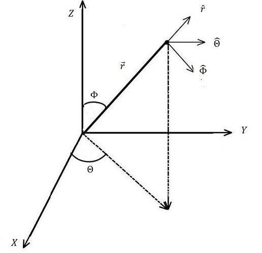
Figure 1: Spherical coordinates used in the derivation of the equations of motion

2 Total Torque due Lorentz Force

We use spherical coordinates to describe the magnetic and gravitational fields, and the spacecraft trajectory, as shown in Figure (1). The $X$, $Y,$ and $Z$ axes form a set of inertial cartesian coordinates. The Earth is assumed to rotate about the $Z$-axes. The magnetic dipole is not tilted and therefore, axi-symmetric. The spherical coordinates consist of radius r, colatitude angle $\Phi$, and azimuth from the $X$ direction $\Theta$ (see Figure. 1). The magnetic field is expressed as

$$\vec{B}\mathbf{=}\frac{B_{0}}{r^{3}}\left[2\cos\Phi~{}\hat{r}\mathbf{+}\sin\Phi~{}\hat{\Phi}\mathbf{+0}\hat{\Theta}\right],$$ (4)

where $B_{0}$ is the strength of the magnetic field in Wb m. The acceleration in inertial coordinates is given by

$$\vec{a}\mathbf{=}\frac{\vec{F}}{m}=-\frac{\mu}{r^{3}}\vec{r}\mathbf{+}\frac{q}{m}(\vec{E}+\vec{V}_{rel}\times\vec{B}\mathbf{),}$$ (5)

where $\frac{q}{m}$is the charge-to-mass ratio of the spacecraft, $\vec{V}_{rel}$ is the velocity of the spacecraft relative to the magnetic field of The Earth. The total Lorentz force (per unit mass) can be written as:

$$\vec{F_{L}} = \frac{q}{m}\left[\vec{E}+\vec{V}_{rel}\times\vec{B}\right]=\frac{q}{m}\vec{E}+\frac{q}{m}(\vec{V}_{rel}\times\vec{B}\mathbf{)}$$ (6)

$$= \vec{F}_{elec}+\vec{F}_{mag},$$

where $\vec{F}_{mag}$ is the Lorentz force experienced by magnetic field and $F_{elec}$ is the Lorentz force experienced by an electric dipole moment in the presence of electric field,

$$\vec{F}_{elec}=\frac{q}{m}\vec{E}.$$ (7)

Now we start with $\vec{F}_{mag}$ using Maxwell (1861), we can write

$$\vec{F}_{mag}=\frac{q}{m}(\vec{V}_{rel}\times\vec{B}\mathbf{),}\vec{V}_{rel}=\vec{V}-\vec{\omega_{e}}\times\vec{r},$$ (8)

where $\vec{V}$ is the inertial velocity of the spacecraft, $\mathbf{\omega}_{e}~{}$is the angular velocity vector of the Earth. According to Gangestad et al. (2010), we used

$$\vec{V}\mathbf{=}~{}\dot{{r}}~{}\hat{r}\mathbf{+}{r}\dot{\Phi}\hat{\Phi}\mathbf{+}{r}\mathbf{~{}}\dot{\Theta}\sin{\Phi}~{}\hat{\Theta},$$

and

$$\vec{r}\mathbf{~{}=}r\mathbf{~{}}\hat{r},~{}\vec{\omega_{e}}=\omega_{e}~{}\hat{z},~{}\hat{z}~{}=\cos\Phi~{}\hat{r}\mathbf{+}\sin\Phi\mathbf{~{}}\hat{\Phi}.$$ (9)

Therefore the acceleration in inertial coordinates is given by

$$\vec{F}_{mag}=\frac{qB_{0}}{m~{}r^{2}}\left[\begin{array}[]{c}-\left(\dot{\Theta}-\omega_{e}\right)\left(\sin^{2}\Phi~{}\hat{r}+\sin(2{\Phi})\hat{\Phi}\right)\\ +\left(\frac{\dot{r}}{r}\sin\Phi-2\dot{\Phi}~{}\cos\Phi\right)\hat{\Theta}\end{array}\right].$$ (10)

In the case of Torque we need the perturbing force $\vec{F}_{L}$ decomposed into radial, transverse, and normal direction. The unit vector $\hat{n}$ normal to the orbit is collinear with the angular momentum unit vector $\hat{h}$.

$$\hat{n}=\hat{h}=\left(\vec{r}\times\vec{V}\right)/\sqrt{\mu p}=r^{2}/\sqrt{\mu p}(-\dot{\Theta}\sin\Phi\hat{\Phi}+\dot{\Phi}\hat{\Theta}),$$ (11)

where $p=a(1-e^{2})$, $\mu$ is the Earth’s gravitational parameter, $a$ is the semi-major axis, $e$ is the eccentricity of the spacecraft orbit, and the transverse unit vector $\hat{t}$ can be calculated from the right-handed set, $\hat{t}=\hat{n}\times\hat{r}$. Decomposition of the Lorentz force experienced by the geomagnetic field into the radial, transverse, and normal components $\left(R_{mag},T_{mag},~{}N_{mag}\right)$ respectively yields,

$$R_{mag}=\vec{F}_{mag}\cdot\hat{r}~{}=\frac{q}{m}\frac{B_{0}}{~{}r^{2}}\left[\omega_{e}-\dot{\Theta}\right]\sin^{2}\Phi,$$ (12)

$$T_{mag}=\vec{F}_{mag}\cdot\hat{t}~{}=\frac{q}{m}\frac{B_{0}}{~{}\sqrt{\mu p}}\left[\begin{array}[]{c}\frac{\dot{r}}{r}\dot{\Theta}\sin^{2}\Phi\\ -2\omega_{e}~{}\dot{\Phi}\cos\Phi\sin\Phi\end{array}\right],$$ (13)

$$N_{mag}=\vec{F}_{mag}\cdot\hat{n}~{}=\frac{q}{m}\frac{B_{0}}{~{}\sqrt{\mu p}}\left[\begin{array}[]{c}2\dot{\Theta}(\omega_{e}-\dot{\Theta})\sin^{2}\Phi\cos\Phi{}\\ +\frac{\dot{r}}{r}\dot{\Theta}\sin\Phi-2\dot{\Phi}^{2}~{}\cos\Phi\end{array}\right].$$ (14)

The relationship between the spherical coordinates and the orbital elements is required to derive the components of Lorentz force experienced by magnetic part as a function of orbital elements.

$$r=p/\left(1+e~{}\cos f\right),~{}\dot{r}=e\sqrt{\mu/p}\sin f,$$ (15)

$$\cos\Phi=\sin i\sin\left(\omega^{\ast}+f\right),\sin\Phi=\sqrt{1-\sin^{2}i\sin^{2}\left(\omega^{\ast}+f\right)},$$ (16)

$$\dot{\Phi}=-\sqrt{\mu/p^{3}}\frac{\sin i\cos\left(\omega^{\ast}+f\right)}{\sqrt{1-\sin^{2}i\cos^{2}\left(\omega^{\ast}+f\right)}}\left(1+e~{}\cos f\right)^{2},$$ (17)

$$\dot{\Theta}=\sqrt{\mu/p^{3}}\frac{\cos i~{}}{1-\sin^{2}i\sin^{2}\left(\omega^{\ast}+f\right)}\left(1+e~{}\cos f\right)^{2},$$ (18)

where $i$, $\omega^{\ast}$ and $f$ are the inclination of the orbit on the equator, argument of the perigee, and the true anomaly of the spacecraft orbit respectively. Therefore, rewriting the components of the magnetic part of the Lorentz force as a function of orbital elements, we obtain

$$R_{mag}=\frac{q}{m}\frac{B_{0}}{~{}r^{2}}\left[\begin{array}[]{c}\omega_{e}(1-\sin^{2}i\sin^{2}\left(\omega^{\ast}+f\right))\\ -\sqrt{\mu/p^{3}}\cos i~{}\left(1+e~{}\cos f\right)^{2}\end{array}\right],$$ (19)

$$T_{mag}=\frac{q}{m}\frac{B_{0}}{~{}\sqrt{\mu p}}\left[\begin{array}[]{c}\frac{\dot{r}}{r}\sqrt{\mu/p^{3}}\cos i~{}\left(1+e~{}\cos f\right)^{2}+2\omega_{e}~{}\sqrt{\mu/p^{3}}\sin^{2}i\sin\left(\omega^{\ast}+f\right)\\ \times\cos\left(\omega^{\ast}+f\right)\left(1+e~{}\cos f\right)^{2}\end{array}\right],$$ (20)

$$N_{mag} = \frac{q}{m}\frac{B_{0}}{~{}\sqrt{\mu p}}\times$$ (25)

$$\left(\begin{array}[]{c}2\left(\omega_{e}(1-\sin^{2}i\sin^{2}\left(\omega^{\ast}+f\right))-\sqrt{\mu/p^{3}}\cos i~{}\left(1+e~{}\cos f\right)^{2}\right)\\ \sqrt{\mu/p^{3}}\cos i~{}\left(1+e~{}\cos f\right)^{2}~{}+\frac{\dot{r}}{r}\sqrt{\mu/p^{3}}\frac{\cos i~{}}{\sqrt{1-\sin^{2}i\sin^{2}\left(\omega^{\ast}+f\right)}}\times\\ \left(1+e~{}\cos f\right)^{2}-2\frac{\mu}{p^{3}}\frac{\sin^{3}i\cos^{2}\left(\omega^{\ast}+f\right)\sin\left(\omega^{\ast}+f\right)}{1-\sin^{2}i\cos^{2}\left(\omega^{\ast}+f\right)}\left(1+e~{}\cos f\right)^{4}\end{array}\right).$$

Now we develop the Lorentz force experienced by electric field $F_{elec}.$

According to Ulaby (2005) and Heilmann et al. (2012) we can write the electric force as follows.

$$\vec{F}_{elec}=-\nabla\vec{V}_{elec}=\left(\frac{\partial~{}V_{elec}}{\partial r}\hat{r}\mathbf{+}\frac{1}{r}\frac{\partial~{}V_{elec}}{\partial\Phi}\hat{\Phi}\mathbf{+}\frac{1}{r\sin\Theta}\frac{\partial~{}V_{elec}}{\partial\Theta}\hat{\Theta}\right),$$ (26)

where $\vec{V}_{elec}$ is the electric potential,

$$V_{elec}=\frac{\vec{P}\cdot\hat{r}}{4\pi~{}\epsilon_{o}r^{2}}.$$ (27)

$\vec{P}=q\vec{d}$ is called the electric dipole moment, $\vec{d}$ is the distance vector from charge $-q$ to charge $+q$, $\epsilon_{o}=8.85\times 10^{-12}$ coul${}^{2}/(N-m^{2})\equiv volt^{-1}meter^{-1}$ is the permittivity of free space. Then the final form of the Lorentz force experienced by an electric dipole moment in the presence of electric field is

$$\vec{F}_{elec}=\frac{qd}{4\pi~{}\epsilon_{o}r^{3}}\left(2\cos\Phi~{}\hat{r}\mathbf{+}\sin\Phi~{}\hat{\Phi}\mathbf{+0~{}}\hat{\Theta}\right).$$ (28)

Similarly as we did for the magnetic force, we can write the radial, transverse, and normal components $\left(R_{elec},T_{elec},~{}N_{elec}\right)$ of the electric force,

$$R_{elec}=-\frac{q}{m}\frac{d}{4\pi~{}\epsilon_{o}r^{3}}\left(\omega_{e}-\dot{\Theta}\right)\sin^{2}\Phi.$$ (29)

$$T_{elec}=\vec{F}_{elec}\cdot\hat{t}~{}=\frac{q}{m}\frac{d}{4\pi~{}\epsilon_{o}r^{3}}\frac{r^{3}}{\sqrt{\mu~{}a\left(1-e^{2}\right)}}\left(\omega_{e}-\dot{\Theta}\right)~{}\dot{\Phi}\sin\Phi~{}\cos\Phi.$$ (30)

$$N_{elec} = \vec{F}_{elec}\cdot\hat{n}~{}$$

$$= \frac{q}{m}\frac{d}{4\pi~{}\epsilon_{o}r^{3}}\frac{r^{2}}{\sqrt{\mu~{}a\left(1-e^{2}\right)}}\left(\omega_{e}-\dot{\Theta}\right)~{}\dot{\Theta}~{}\sin^{2}\Phi~{}\cos\Phi.$$

Similarly, we can write the components of the Lorentz force experienced by an electric field as a function of orbital elements as follows.

$$R_{elec}=-\frac{q}{m}\frac{d}{4\pi~{}\epsilon_{o}r^{3}}\left[\begin{array}[]{c}\omega_{e}\left(1-\sin^{2}i\sin^{2}\left(\omega^{\ast}+f\right)\right)-\\ \sqrt{\mu/a^{3}\left(1-e^{2}\right)^{3}}~{}\cos i~{}\left(1+e~{}\cos f\right)^{2}\end{array}\right].$$ (32)

$$T_{elec} = \frac{q}{m}\frac{d}{4\pi~{}\epsilon_{o}r^{2}}\times$$

$$\left(\omega_{e}-\sqrt{\mu/a^{3}\left(1-e^{2}\right)^{3}}\frac{\cos i~{}\left(1+e~{}\cos f\right)^{2}}{1-\sin^{2}i\sin^{2}\left(\omega^{\ast}+f\right)}\right)\sin^{2}i\cos\left(\omega^{\ast}+f\right)\sin\left(\omega^{\ast}+f\right).$$

$$N_{elec} = \frac{q}{m}\frac{d}{4\pi~{}\epsilon_{o}r^{3}}\times$$

$$\left(\omega_{e}-\sqrt{\mu/a^{3}\left(1-e^{2}\right)^{3}}\frac{\cos i~{}\left(1+e~{}\cos f\right)^{2}}{1-\sin^{2}i\sin^{2}\left(\omega^{\ast}+f\right)}\right)\sin i~{}\cos i\sin\left(\omega^{\ast}+f\right)~{}.$$

Assuming that the spacecraft is equipped with a charged surface (screen) of area $S$ with the electric charge $q=\int_{{S}}\sigma\,dS$ distributed over the surface with density $\sigma$. Therefore, as in Tikhonov et al. (2011), we can write the torque of these forces relative to the spacecraft’s center of mass as follows.

$${\vec{T}}_{{L}}=\vec{T}_{mag}+\vec{T}_{elec}=\int_{S}{\sigma}{\vec{\rho}}\times(\vec{E}+\vec{V}\times{\vec{B})}{dS},$$ (35)

where $\vec{\rho}$ is the radius vector of the screen’s element $dS$ relative to the spacecraft’s center of mass and $\vec{V}$ is the velocity of the element $dS$ relative to the geomagnetic field. Finally, the torque due to Lorentz force can be written as follows

$$\vec{T}_{mag}=\vec{\rho}_{{0}}\times{A}^{T}\left(R_{mag},T_{mag},~{}N_{mag}\right)^{T},\vec{T}_{elec}=\vec{\rho}_{{0}}\times{A}^{T}\left(R_{elec},T_{elec},~{}N_{elec}\right)^{T},$$ (36)

$${\vec{\rho}}_{{0}}{=x}_{{0}}{i}_{{b}}{+y}_{{0}}{j}_{{b}}{+z}_{{0}}k_{{b}}{=}q^{-1}\int_{{S}}\sigma\,\vec{\rho}\,dS$$ (37)

$\vec{\rho}_{{0}}$ is the radius vector of the charged center of a spacecraft relative to its center of mass and $A^{{T}}$ is the transpose of the matrix ${A.}$

2.1 Geomagnetic field model and its Torque

In this paper we are using non-tilted dipole for the geomagnetic field. Let a dipole magnetic field be $\vec{B}=(B_{1},B_{2},B_{3}),$ and the magnetic moment be $\vec{M}=(m_{1},m_{2},m_{3})$ of the spacecraft. Therefore the torque due to the geomagnetic field is

$$\vec{T}_{M}=\vec{M}\times\vec{B}$$ (38)

As in Wertz (1978) we can write geomagnetic field and the total magnetic moment of the orbital system directed to the tangent of the orbital plane, normal to the orbit, and in the direction of the radius respectively as below:

$$B_{1} = \frac{B_{0}}{2r^{3}}\sin\theta_{m}^{\prime}\,[3\cos(2f-\alpha_{m})+\cos\alpha_{m}],\text{ }B_{2}=-\frac{B_{0}}{2r^{3}}\,\cos\theta_{m}^{\prime}\,,$$ (39)

$$B_{3} = \frac{B_{0}}{2r^{3}}\sin\theta_{m}^{\prime}\,[3\sin(2f-\alpha_{m})+\sin\alpha_{m}].$$ (40)

$$m_{1}=m\,\sin\theta_{m}^{\prime}\cos\alpha_{m}\,{\beta_{1}},~{}m_{2}=m\,\sin\theta_{m}^{\prime}\sin\alpha_{m}\,{\beta_{2}},\text{ }m_{3}=m\,\cos\theta_{m}^{\prime}\,{\beta_{3}},$$ (41)

where $B_{0}=-8\times 10^{-15}$, $\theta_{m}^{\prime}=168.6^{\circ}$ is the co-elevation of the dipole, $\alpha_{m}=109.3^{\circ}$, is the east longitude of the dipole and $f$ is the true anomaly measured from ascending node and $m$ is the magnitude of the total magnetic moment.

3 Equations of the attitude motion

The nonlinear differential equation called Euler-Poisson  equations are used to describe the attitude orientation of the spacecraft.

$${\ }\dot{\vec{\omega}}I+\vec{\omega}\times\vec{\omega}I=\vec{T}_{G}+\vec{T}_{M}+\vec{T}_{L},$$ (42)

$$\dot{\vec{\alpha}}+\vec{\alpha}\times\vec{\omega}\mathbf{=-}\Omega\vec{\gamma},\dot{\vec{\beta}}+\vec{\beta}\times\vec{\omega}=0,\,\,\,\,\,\,\,\dot{\vec{\gamma}}+\vec{\gamma}\times\vec{\omega}=\Omega\vec{\alpha}$$ (43)

where $\vec{T}_{G}=3\Omega^{2}\vec{\gamma}\times\vec{\gamma}I$ is the well known formula of the gravity gradient torque,

$I={diag}(A,B,C)$ is the inertia matrix of the spacecraft, $\Omega$ is the orbital angular velocity, $\vec{\omega}$ is the angular velocity vector of the spacecraft. According to Wertz (1978) the angular velocity of the spacecraft in the inertial reference frame is $\vec{\omega}=(p,q,r)\mathrm{,}$ where

$$p={\dot{\psi}\sin\theta\sin\phi+\dot{\theta}\,\cos\phi,}q={\dot{\psi}\sin\theta\cos\phi-\dot{\theta}\,\sin\phi,}r={\dot{\psi}\cos\theta+\dot{\phi}.}$$ (44)

3.1 Equations of motion in the pitch direction

In this section the attitude motion of the spacecraft in the pitch direction is considered, i.e. $\psi=\phi=0,~{}\theta\neq 0.$ Applying this condition in equation (42), we can derive the second order differential equation of the motion in pitch direction.

$${A}\frac{d^{2}\theta}{dt^{2}} = (C-B)(3\Omega^{2}-1){\sin\theta\cos\theta}+z_{0}{\sin\theta}(~{}N_{mag}-kT_{mag})$$

$$+z_{0}{\cos\theta}(kN_{mag}-T_{mag}){+}z_{0}{\sin\theta}(~{}N_{elec}-kT_{elec})$$

$$+z_{0}{\cos\theta}(kN_{elec}-T_{elec})+{m_{2}B}_{3}{\sin\theta+m_{3}B}_{2}{\cos\theta.}$$

Let $y_{0}=k~{}z_{0},$where $k$ is arbitrary number.

$$A\ddot{\theta} = \left(3\Omega^{2}-1\right)(C-B)\sin\theta\cos\theta+z_{0}\sin\theta(N_{mag}-kT_{mag})$$ (46)

$$+z_{0}\cos\theta(kN_{mag}-T_{mag})+z_{0}\sin\theta(N_{elec}-kT_{elec})$$

$$+z_{0}\cos\theta(kN_{elec}-T_{elec})+B_{2}m_{3}\sin\theta+B_{3}m_{2}\cos\theta$$

$$= g(k,z0,\alpha^{\ast}=q/m,\theta),$$

where $N_{mag},T_{mag},N_{elec},T_{elec}$ are given in equations (20), (25), (2) and (2) respectively.

A comparison in the oscillation of  $\overset{.}{{\theta}}$ is given in figures (2) to (3). It is obvious from the first two figures that the most significant amount of torque is coming from the magnetic part of the Lorentz torque which is of the order $10^{-3}$. The effect from electric part of the Lorentz torque is of the order $10^{-11}$ which is very small. The contribution from geomagnetic torque is of the order $10^{-6}$.  The oscillation in $\overset{.}{{\theta}}$ due to total Torque is of the order $10^{-3},$ as shown in figure (3 right). As the contribution from the electric part of Lorentz force and geomagnetic field is very small compared to the magnetic part of Lorentz force therefore it doesn’t show up in figure (3 left). These figures are drawn for fixed values of $B=0.7$, $C=0.1$, $\alpha^{\ast}=\pm 1$.

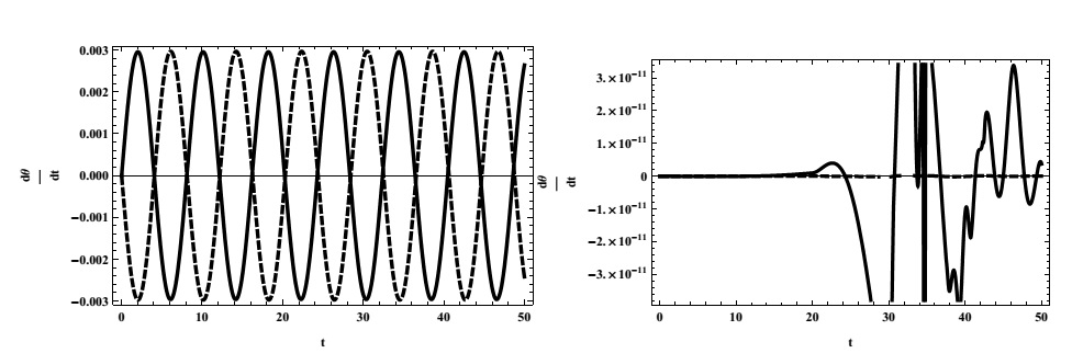
Figure 2: Oscillation in $\frac{d\theta}{dt}$ due to (left) magnetic part from Lorentz Torque and (right) due to electric part from Lorentz Torque. The dotted line corresponds to $\alpha^{*}=-0.1$ and the continuous line corresponds to $\alpha^{*}=0.1$

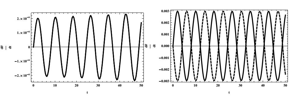
Figure 3: Oscillation in $\frac{d\theta}{dt}$ due to (left) geomagnetic torque and (right) Torque due to total Lorentz force and geomagnetic field. The dotted line corresponds to $\alpha^{\ast}=-0.1$ and the continuous line corresponds to $\alpha^{\ast}=0.1$. Both the lines for $\alpha^{\ast}=\pm 0.1$ are overlapping.

3.2 Derivation of equilibrium solutions in the pitch direction and their linear stability analysis

In this section the existence and stability of equilibrium position in the pitch direction of a general shape spacecraft under the influence of gravitational torque, Lorentz torque, and geomagnetic torque will be discussed. The stability of the equilibrium solutions derived will be discussed both analytically and numerically. To find the equilibrium solutions, take the right hand side of equation (46) equal to zero which reduces to the following equation for $B=0.7,C=0.1,$ $a=6900km,i=51^{\circ},e=0.001,$ and $f=60^{\circ}.$

$$g(k,z0,\alpha^{\ast},\theta) = (2.34\times 10^{-7}+(0.015+0.008k)z_{0}\alpha^{\ast})\cos\theta$$

$$+(1.56\times 10^{-6}+(0.008+0.015k)z_{0}\alpha^{\ast})\sin\theta+0.3\sin 2\theta=0.$$

It is not possible to solve equation (3.2) in closed form as $\theta=f(k,z_{0},\alpha^{\ast})$ therefore numerical techniques are used to identify all the roots of equation (3.2). As equation (46) is derived by taking$\ y=kz_{0},$ therefore without loss of generality we take $z_{0}=1.$ For $0<\alpha^{\ast}<1$ and $0<k<1,$ we have five equilibrium solutions at $\theta\approx\frac{n\pi}{2},n=0,1,2,3,4$ when $\theta\in[0,2\pi].$ As $g(k,\alpha^{\ast},\theta)$ is a periodic function of period $2\pi$ therefore it is sufficient to investigate the equilibrium solutions from $0$ to $2\pi.$ For $0<\alpha^{\ast}<1$ and $k\leq 100$ there are five equilibrium solutions which reduces to three or two when $k>100$. For sufficiently high values of $\alpha^{\ast},$ the number of equilibrium solutions can be reduced to three for even smaller values of $\alpha^{\ast}.$ To see the progression of roots from five to three see figures (4) where $g(k,\alpha^{\ast},\theta)$ is plotted for various fixed values of $k$ and $\alpha^{\ast}.$ To completely describe the progression of the number of equilibrium positions in $[0,2\pi]$ from five to two a 3D implicit plot of $g(k,\alpha^{\ast},\theta)=0$ is given in figure (5). It can easily be seen that for high enough values of $\alpha^{\ast}$ and $k$, the number of equilibrium points reduces to two. It is also obvious from these figures that the equilibrium positions does not always remain at $\theta\approx\frac{n\pi}{2},n=0,1,2...$. By the comparison of figure (4 left) and figure (4 right) it is evident that the equilibrium positions are not the same for positively and negatively charged spacecrafts. It remains to be seen if this or the other parameters such as $\alpha^{\ast}$ or $k$ effect the stability of the equilibrium points.

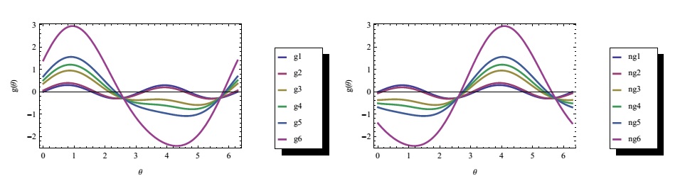
Figure 4: Progression of equilibrium solutions when (left) g1) $(\alpha^{\ast},k)=(0.1,1)$, g2) $(\alpha^{\ast},k)=(2,2)$, g3) $(\alpha^{\ast},k)=(5,7)$, g4) $(\alpha^{\ast},k)=(7,7)$, g5) $(\alpha^{\ast},k)=(7,10)$, g6) $(\alpha^{\ast},k)=(10,15)$ and (right) when ng1) $(\alpha^{\ast},k)=(-0.1,1)$, ng2) $(\alpha^{\ast},k)=(-2,2)$, ng3) $(\alpha^{\ast},k)=(-5,7)$, ng4) $(\alpha^{\ast},k)=(-7,7)$, ng5) $(\alpha^{\ast},k)=(-7,10)$, ng6) $(\alpha^{\ast},k)=(-10,15)$

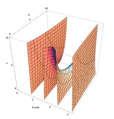
Figure 5: Implicit plot of $g(k,\alpha^{\ast},\theta)=0$ when $z_{0}=1$.

To discus the linear stability of the equilibrium points identified above we use the standard procedure of linearization and convert equation (46) to a system of two first order equations. We then find the eigenvalues of the jacobian matrix from the equation given below.

$$\lambda^{2}-\frac{\partial g(k,z0,\alpha^{\ast},\theta)}{\partial\theta}=0,$$ (48)

where

$$\frac{\partial g(k,z0,\alpha^{\ast},\theta)}{\partial\theta} = A^{-1}({\cos\theta(1.56\times 10^{-6}+10^{-3}(8+}{15k)z_{0}\alpha^{\ast})}$$

$${+(B-C)\cos(2\theta)}{-\sin\theta(2.34\times 10^{-7}+10^{-3}(15}{+8k)z_{0}\alpha^{\ast})}.$$

It is clear from equation (48) that there are only two types of eigenvalues possible. If $g_{\theta}(k,z0,\alpha^{\ast},\theta)>0$ there will be two eigenvalues one of which is negative and one positive. A positive eigenvalue always imply instability. If $g_{\theta}(k,z0,\alpha^{\ast},\theta)<0$ the eigenvalues obtained will be imaginary with a zero real part which means the equilibrium point in question will be spectrally stable. Initially we will investigate the equilibrium points obtained above for $A=1,B=0.7,C=0.1,z_{0}=1.$

$$\frac{\partial g(k,\alpha^{\ast},\theta)}{\partial\theta} = g_{\theta}={\cos\theta(1.56\times 10^{-6}+10^{-3}(8+15k)\alpha^{\ast})}{+0.6\cos(2\theta)}$$ (50)

$$-{\sin\theta(2.34\times 10^{-7})}{+10^{-3}\sin\theta(15+8k)\alpha^{\ast}.}$$

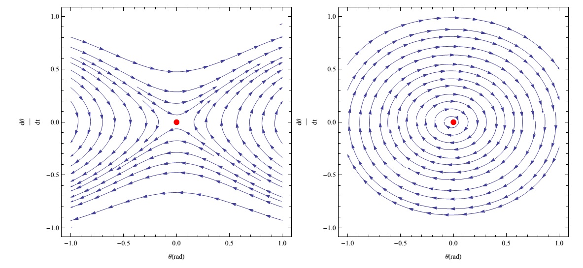
Figure 6: Trajectory in the $\theta$-$\frac{d\theta}{dt}$ phase plane when (left) $\alpha^{\ast}=0.01,k=1,z_{0}=1,A=1,B=0.7,C=0.1$,(right) $\alpha^{\ast}=-1,k=100,z_{0}=1,A=1,B=0.7,C=0.1$.

The values of $g_{\theta}|_{\theta=0}$ and $g_{\theta}|_{\theta=2\pi}$ remain positive for all positive values of $k$ and $\alpha^{\ast}$ which implies that the equilibrium position at $\theta=0$ and $\theta=2\pi$ are unstable. The value of $g_{\theta}|_{\theta=\pi/2}$ is negative for all positive values of $k$ and $\alpha^{\ast}$ which implies that the equilibrium position at $\theta=\pi/2$ will be stable. By similar argument, the equilibrium position at $\theta=\pi$ will be stable if $\alpha^{\ast}$ satisfy the following inequality.

$$\alpha^{\ast}>\frac{0.6}{0.008+0.015k}=\alpha_{1}^{\ast}.$$

This also means that $\theta=\pi$ will always be unstable if the spacecraft is negatively charged as the right hand side of the above inequality is always positive. To check the stability of the remaining four equilibrium positions when $\alpha^{\ast}<0,$ Let $\alpha^{\ast}=-\alpha_{p}$ such that $\alpha_{p}>0.$ It can easily be shown that the equilibrium position at $\theta=0$ and $\theta=2\pi$ will be stable if $\alpha_{p}<\alpha_{1}^{\ast}.$ For example when $k=1,$ $\alpha_{p}$ must be smaller than $26.09.$ Similarly, for the equilibrium position at $\theta=\pi/2$ to be stable for negatively charged spacecraft $\alpha_{p}$ must satisfy the following inequality.

$$\alpha_{p}<\frac{0.6}{0.008k+0.015}.$$

It can be safely concluded from this discussion that the sign and amount of charge on the spacecraft plays a significant role in the stability of the equilibrium positions. A typical trajectory in the $\theta$-$\frac{d\theta}{dt}$ phase plane around $\theta=0$ is given in figure ( 6) for $\alpha^{\ast}=0.01,-1,$ $k=1,100,$ $z_{0}=1,$ $A=1,$ $B=0.7,$ $C=0.1$. It can be seen that all the trajectories are moving away from $\theta=0$ when $\alpha^{\ast}=0.01,$ which indicate instability. In the second case it is stable.

Figure 7: A set of orbits with initial positions close to $(\theta,\dot{\theta)}\rightarrow(0+,0+)$ in the $\theta$-$\frac{d\theta}{dt}$ phase plane when $\alpha^{\ast}=0.01,k=1,z_{0}=1,A=1,B=0.7,C=0.1$

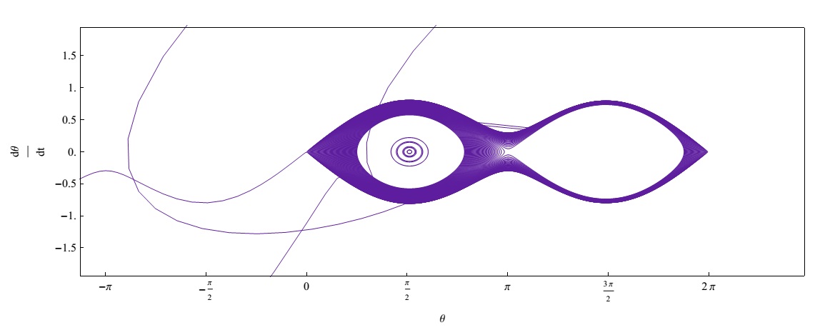
Figure 8: Same orbits as in figure (7) but integrated for much longer time.

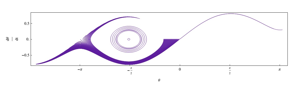
Figure 9: A set of orbits with initial positions close to $(\theta,\dot{\theta})\rightarrow(0-,0-)$ in the $\theta$-$\frac{d\theta}{dt}$ phase plane when $\alpha^{\ast}=0.01,k=1,z_{0}=1,A=1,B=0.7,C=0.1$

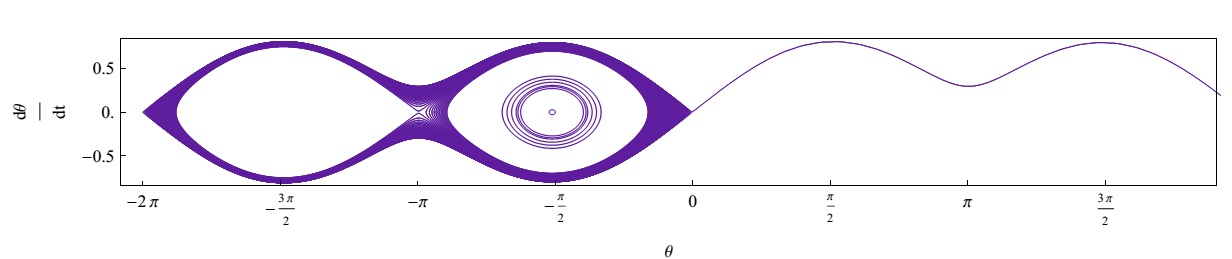
Figure 10: Same orbits as in figure (9) but integrated for much longer time.

To understand the long term behavior of orbits around the equilibrium positions a set of orbits with initial positions close to $(\theta,\dot{\theta)}\rightarrow(0+,0+)$ and $(\theta,\dot{\theta)}\rightarrow(\frac{\pi}{2},0)$ are given in figures ( 7, 8) in the $\theta$-$\frac{d\theta}{dt}$ phase plane when $\alpha^{\ast}=0.01,k=1,z_{0}=1,A=1,B=0.7,C=0.1$. These orbits are allowed to evolve for a short period of time and their trajectories are traced in figure ( 7). It can be seen that the orbits starting close to $0+$ (close to 0 and positive) are immediately captured by the nearby stable equilibrium at $\frac{\pi}{2}.$ The orbits which start near $(\theta,\dot{\theta)}\rightarrow(\frac{\pi}{2},0)$ remain in elliptic orbit around $(\frac{\pi}{2},0).$ When these orbits are allowed to evolve for a longer period of time some of the orbits near $(0+,0+)$ are being captured by the nearby stable equilibrium at $\frac{3\pi}{2}$ and a couple of orbits escapes. The orbits close to $(\frac{\pi}{2},0)$ remain in near circular orbit about the center which is a strong evidence of the existence of periodic orbits around $(\frac{\pi}{2},0).$ Similar analysis is performed for orbits with initial positions close to $(\theta,\dot{\theta)}\rightarrow(0-,0-)$ and $(\theta,\dot{\theta)}\rightarrow(-\frac{\pi}{2},0).$ It can be seen in figures ( 9, 10) that the orbits starting close to $0-$ (close to 0 and negative) are immediately captured by the nearby center at $-\frac{\pi}{2}.$ Some of them when integrated for a much longer period of time gets captured by the center at $\frac{-3\pi}{2}.$ The orbits which start around $(-\frac{\pi}{2},0)$ remain in near circular orbits around $(-\frac{\pi}{2},0).$ Similar behavior is observed around all the spectrally stable equilibriums. Therefore we can safely conjecture that around each stable equilibrium position there is a family of periodic orbits.

As mentioned earlier and shown in figures (4) and (5) the number of equilibrium points  when $0<\theta<2\pi$ reduce from five to three and in some cases two for higher values of $\alpha^{\ast}$ and $k.$ For example when $B=0.7,C=0.1,k=10,z_{0}=1,$ and $\alpha^{\ast}=7$ there are two equilibrium points at $\theta=2.32$ (stable)$,5.89$ (unstable). If $\alpha^{\ast}=-7$ i.e. the spacecraft is negatively charged, the position of the two equilibriums are changed and the stability reversed. When $|B-C|<1$, the positions of the equilibrium points are almost identical to what we have shown above. Its effect on stability is explained below.

1. $\theta=0,2\pi$: When $B\geq C$ and $\alpha^{\ast}>0,$ the equilibrium positions at $\theta=0,2\pi$ will be stable. But when $\alpha^{\ast}<0$ these two equilibrium positions are unstable.

2. $\theta=\frac{\pi}{2}$: For $B\geq C$ the equilibrium position at $\theta=\frac{\pi}{2}$ is always stable. However, when $B<C$ the value of $\alpha^{\ast}$ have to be significantly high in which case $\theta=\frac{\pi}{2}$ will no more be an equilibrium position.

3. $\theta=\pi:$When $B\leq C$ and $\alpha^{\ast}>0,$ $\theta=\pi$ is stable. For    a negatively charged spacecraft $B<C$ is a necessary condition for the stability of the equilibrium position at $\theta=\pi.$ Therefore when $B>C,$ the value of $\alpha^{\ast}$ have to be significantly high in which case $\theta=\pi$ will no more be an equilibrium position.

4. $\theta=\frac{3\pi}{2}:B>C$ is a necessary and sufficient condition for the stability of the equilibrium position at $\theta=\frac{3\pi}{2}$ unless $\alpha^{\ast}$ is very large and negative in which case $\theta=\frac{3\pi}{2}$ will no more be at equilibrium position.

In summary, when $0<\alpha^{\ast}<1$ and $B<C,$ the equilibrium positions at $\theta=0,\pi,2\pi$ are stable and at $\theta=\frac{\pi}{2},\frac{3\pi}{2}$ are unstable and when $B>C$ the nature of the five equilibrium positions is reversed. To demonstrate this behavior a typical example is given in figure (11)

Figure 11: Trajectory in the $\theta$-$\frac{d\theta}{dt}$ phase plane when $\alpha=0.01,k=1,z_{0}=1$ and  (Left): $B=0.5,C=0.9$. (Right): $B=0.9,C=0.5$. Black dots correspond to stable equilibrium points and red dots correspond to unstable equilibrium points.

3.3 Equations of motion in the roll direction

In this section we study the attitude motion of the spacecraft in the roll direction, i.e. $\psi=\theta=0,~{}\phi\neq 0.$ Applying this condition in Euler equation of the attitude motion of the spacecraft, we obtain the second order differential equation of the motion in roll direction.

$${C}\frac{d^{2}{\phi}}{dt^{2}} = \Omega^{2}(A-B){\sin\phi\cos\phi}+x_{0}{\sin\phi}(kT_{mag}-~{}R_{mag})+x_{0}{\cos\phi}(T_{mag}-kR_{mag})$$

$$+x_{0}{\sin\phi}(kT_{elec}-~{}R_{elec})+x_{0}{\cos\phi(T_{elec}}{-~{}kR_{elec})+m_{1}B}_{2}{\cos\phi-{m_{2}B}_{1}\sin\phi.}$$

Let ${y}_{{0}}=k{x}_{{0}}~{}$meter then,

$${\ C}\frac{d^{2}{\phi}}{dt^{2}} = \Omega^{2}(A-B){\sin\phi\cos\phi}+x_{0}{\sin\phi}(kT_{mag}-~{}R_{mag})+x_{0}{\cos\phi}(T_{mag}-kR_{mag})$$ (51)

$${+}x_{0}{\sin\phi}(kT_{elec}-~{}R_{elec})+x_{0}{\cos\phi(T_{elec}}{-~{}kR_{elec})\cos\phi+m_{1}B}_{2}{\cos\phi-{m_{2}B}_{1}\sin\phi}$$

$$= h(\alpha^{\ast},k,{\phi,x}_{0},{A,B).}$$

3.4 Derivation of equilibrium solutions in Roll direction and their linear stability analysis

In this section the existence and stability of equilibrium positions in the roll direction of a general shape spacecraft under the influence of gravitational torque, Lorentz torque, and geomagnetic torque will be discussed. The stability of the equilibrium positions derived will be discussed both analytically and numerically. To find the equilibrium positions, take the right hand side of equation (51) equal to zero which reduces to the following equation for $A=0.1,B=0.7,C=1,$ $x_{0}=1,$ $a=6900km,i=51^{\circ},e=0.001,$ and $f=60^{\circ}.$

$$h_{1}(k,\alpha^{\ast},\phi)=(1.036\times 10^{-7}+(-0.012+9.41k)\alpha^{\ast}) \times\cos\phi+(-1.13\times 10^{-7}$$

$$+9.41\times 10^{-10}\alpha^{\ast}-0.012k\alpha^{\ast})\sin\phi -3.63\times 10^{-7}\sin(2\phi)=0.$$ (52)

It is not possible to solve equation $h_{1}(k,\alpha^{\ast},\phi)=0$ in closed form as $\phi=f(k,\alpha^{\ast})$ therefore numerical techniques are used to identify all the roots of equation $h_{1}(k,\alpha^{\ast},\phi)=0$ which are the desired equilibrium solutions. Let $k=1.$ For $\alpha^{\ast}\in(-2.15\times 10^{-5},2.15\times 10^{-5})$ i.e for a very small amount of charge, there are four equilibrium solutions and for higher values of $\alpha^{\ast}$ there are two equilibrium solutions.

1. $\phi_{1}\in(0,0.4)$ when $\alpha^{\ast}\in(-2.15\times 10^{-5},2.15\times 10^{-5}).$

2. $\phi_{2}\in(1.47,1.89)$ when $\alpha^{\ast}\in(-2.15\times 10^{-5},2.15\times 10^{-5}).$

3. $\phi_{3}\in(2.80,3.18)$ when $\alpha^{\ast}\in(-2.15\times 10^{-5},2.15\times 10^{-5}).$

4. $\phi_{4}\in(4.37,4.73)$ when $\alpha^{\ast}\in(-2.15\times 10^{-5},2.15\times 10^{-5})$

5. $\phi_{5}=2.36$ when $\left|\alpha^{\ast}\right|>2.15\times 10^{-5}$

6. $\phi_{6}=5.5$ when $\left|\alpha^{\ast}\right|>2.15\times 10^{-5}$

In the above example $B>A.$ Now we switch the values of $A$ and $B$ to have $B<A$ and find the location of the equilibrium positions. In this case we still have four equilibrium solutions when $\alpha^{\ast}\in(-2.15\times 10^{-5},2.15\times 10^{-5})$ and two when $\left|\alpha^{\ast}\right|>2.15\times 10^{-5}.$ All the equilibrium positions when $A=0.7,$ $B=0.1,k=1,C=1,x_{0}=1,$ $a=6900km,i=51^{\circ},e=0.001,$ and $f=60^{\circ}$ are listed below.

1. $\phi_{7}\in(1.23,1.58)$ when $\alpha^{\ast}\in(-2.15\times 10^{-5},2.15\times 10^{-5}).$

2. $\phi_{8}\in(3.12,3.47)$ when $\alpha^{\ast}\in(-2.15\times 10^{-5},2.15\times 10^{-5}).$

3. $\phi_{9}\in(4.69,5.04)$ when $\alpha^{\ast}\in(-2.15\times 10^{-5},2.15\times 10^{-5}).$

4. $\phi_{10}\in(5.97,6.32)$ when $\alpha^{\ast}\in(-2.15\times 10^{-5},2.15\times 10^{-5})$

5. $\phi_{11}=2.36$ when $\left|\alpha^{\ast}\right|>2.15\times 10^{-5}$

6. $\phi_{12}=5.5$ when $\left|\alpha^{\ast}\right|>2.15\times 10^{-5}$

As ${y}_{0}=kx_{0}$ we can take $x_{0}=1.$ To reduce the dimensions, without loss of generality, we define $ab=A-B$ and rewrite $h_{1}(k,\alpha^{\ast},\phi,ab)$ as below.

$$h_{1}(k,\alpha^{\ast},\phi,ab) = \left(-1.13\times 10^{-7}+10^{-3}(6k-15)\alpha^{\ast}\right){\cos}\phi+1.03\times 10^{-7}$$

$$+10^{-3}(6-15k)\alpha^{\ast}){\sin}\phi+6.05\times 10^{-7}ab{\sin}(2\phi).$$

It can be seen from figure (12) that there are four equilibrium solutions for small values of $\alpha^{\ast}$ and all values of $ab$ when $k=1$. For higher values of $\alpha^{\ast}$ there are only two equilibrium solutions at $\phi=2.3$ and $\phi=5.5$ for all values of $ab$. We have seen above that for $k=1$, the changing values of $ab$ and $\alpha^{\ast}$ have significant effect on the existence of equilibrium solutions in the roll direction. To see this for $k\neq 1$, we plot $h_{1}(k,\alpha^{\ast},\phi,ab)=0$ for fixed values of $ab=0.3,$ and $ab=-0.3$ in figure (13). It is clear from figure (13) that with the changing value of $k$ the position of equilibrium changes significantly but the numbers of equilibrium positions remains four as before both for negative and positive values of $ab$ when $\alpha^{\ast}$ is small. The effect of $ab$ is significant when $k<1.$ For higher values $\alpha^{\ast}$ the number of equilibrium positions remains to be two but their positions change with the changing values of $ab$ and $k,$ see figures (12 and 13).

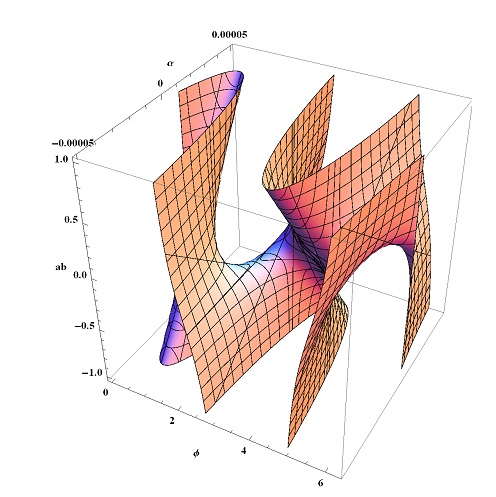
Figure 12: Implicit plots of ( $h(\alpha,\phi,ab)=0$.

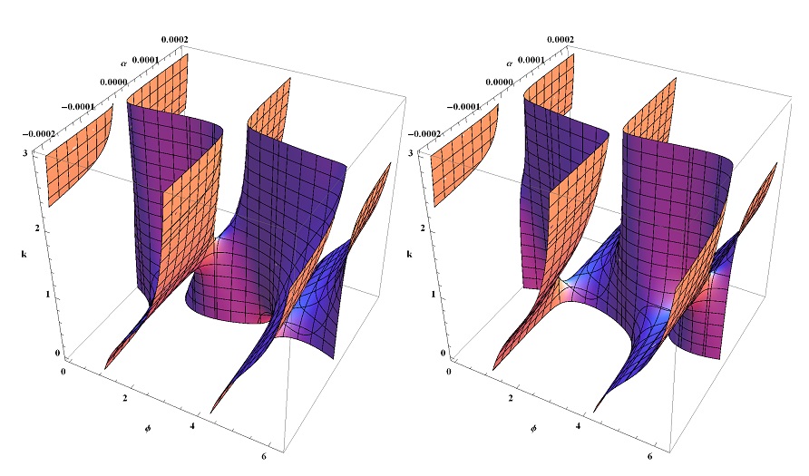
Figure 13: Implicit plots of $h(\alpha,\phi,k,ab)=0$ when (left) $ab=-0.3$ and (right) $ab=0.3$.

To study the stability of the equilibrium position derived we use the same method which was used for the pitch direction. We write equation (51) as a system of two first order equations, linearize them, and find the eigenvalues of the jacobian matrix from the equation given below.

$$\lambda^{2}-h_{\phi}(\alpha^{\ast},k,\phi,ab)=0.$$ (53)

It can be seen from equation (53) that there are only two types of eigenvalues possible. If $h_{\phi}(\alpha^{\ast},k,\phi,ab)>0$ there exist two eigenvalues one of which is negative and one is positive. Therefore $h_{\phi}(\alpha^{\ast},k,\phi,ab)>0$ becomes a sufficient condition for instability. If $h_{\phi}(\alpha^{\ast},k,\phi,ab)<0$ the equilibrium point in question will be spectrally stable or a stable center. We will investigate the equilibrium points obtained above for $ab=0.6,ab=-0.6,k=1,x_{0}=1$,$~{}a=6900km,i=51^{\circ},e=0.001,f=60^{\circ},$ and write $h_{\phi}(\alpha^{\ast},\phi,ab)$ as below.

$$h_{\phi}(\alpha^{\ast},\phi)|_{ab=-0.6} = (-1.13\times 10^{-7}-0.01\alpha^{\ast})\cos\phi-7.26\times 10^{-7}(\cos\phi)^{2}$$

$$+(-1.04\times 10^{-7}+0.01\alpha^{\ast}+7.26\times 10^{-7}\sin\phi)\sin\phi.$$

The equilibrium positions at $\phi_{1}$ and $\phi_{3}$ are stable as in these cases $h_{\phi}(\alpha^{\ast},\phi)|_{ab=-0.6}<0$. Similarly $\phi_{2}$ and $\phi_{4}$ are unstable as in these cases $h_{\phi}(\alpha^{\ast},\phi)|_{ab=-0.6}>0.$ By similar arguments $\phi_{5}$ will be an unstable equilibrium if the spacecraft is positively charged and $\phi_{6}$ will be unstable if the spacecraft is negatively charged. Similarly, when $ab=0.6,$ $\phi_{7}$ and $\phi_{9}$ are stable, $\phi_{8}$ and $\phi_{10}$ are unstable, $\phi_{11}$ is stable when $\alpha^{\ast}<-1.11\times 10^{-6}$ and $\phi_{12}$ is stable when $\alpha^{\ast}>3.25\times 10^{-7}.$ A typical example is given in figure (14) when $ab=\pm 0.6$. The equilibrium at $\phi=2.36$ is stable when $\alpha^{\ast}=-0.1$ and unstable when $\alpha^{\ast}=0.1$. Similarly, the equilibrium at $\phi=5.5$ is unstable when $\alpha^{\ast}=-0.1$ and stable when $\alpha^{\ast}=0.1$.

Figure 14: Trajectory in the $\phi$-$\frac{d\phi}{dt}$ phase plane when (left) $\alpha^{\ast}=0.1,k=1,z_{0}=1,ab=-0.6$,(right) $\alpha^{\ast}=-0.1,k=1,z_{0}=1,ab=-0.6$.

Figure 15: A set of orbits with initial positions close to the equilibrium positions when $e=0.1,ab=0.6$ and (left) $\alpha^{\ast}=-0.1$, (right) $\alpha^{\ast}=0.1$

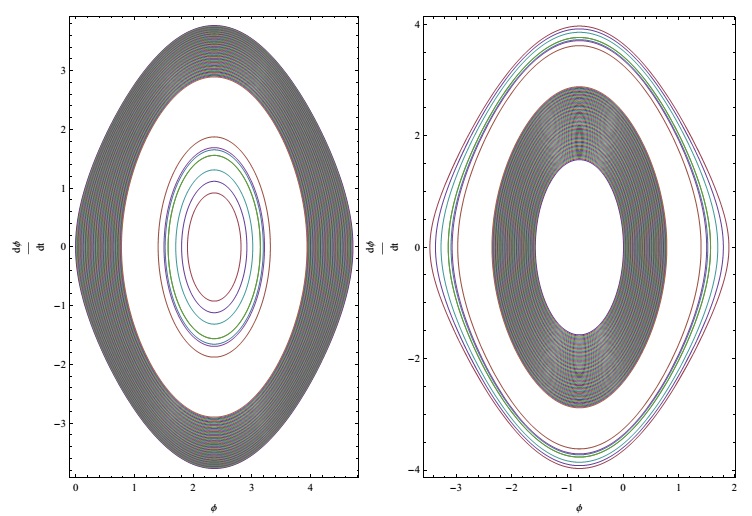
Figure 16: A set of orbits with initial positions close to the equilibrium positions when $e=0.1,ab=0.6$ and (left) $\alpha^{\ast}=-1$, (right) $\alpha^{\ast}=1$

To understand the long term behavior of orbits around the equilibrium positions, a set of orbits with initial positions close to the equilibrium are given in figures ( 15, 16) in the $\phi$-$\frac{d\phi}{dt}$ phase plane when $\alpha^{\ast}=\pm 0.1,\pm 1,$ and $k=1,z_{0}=1,ab=0.6,e=0.1$. These orbits are allowed to evolve for a long period of time and their trajectories are traced in figures (15, 16). The orbits in figure (15left) are given for $\alpha^{\ast}=-0.1$ and it can be seen that all the orbits are captured by the equilibrium position at $\phi=2.36$ which is a stable equilibrium. The orbits which are closer to the stable equilibrium position remain in perfect periodic orbit while the orbits which are not so close have an elliptic orbit in the vicinity of the equilibrium position but are not necessarily periodic. For $\alpha^{\ast}=0.1$ in figure ( 15right), the equilibrium position at $\phi=2.36$ is unstable. Hence the same orbits are captured by another nearby stable equilibrium at $\phi=-0.723$ which is a mirror image of the stable equilibrium at $\phi=5.56$. When the same orbits are integrated for $\alpha^{\ast}=\pm 1$, similar behavior is observed. Also, similar behavior is observed around all the stable equilibriums. Therefore we can safely conjecture that around each stable equilibrium position there is a family of periodic orbits.

4 Conclusions

The paper discussed the attitude stabilization of a charged spacecraft moving in an elliptic orbit using Lorentz torque. The Lorentz torque is developed in two parts $T_{mag}$ and $T_{elec}.$ $T_{mag}$ is the Lorentz torque which is experienced by magnetic field and $T_{elec}$ is the Lorentz Torque experienced by an electric dipole moment in the presence of electric field. The model we developed incorporates all Lorentz torques as a function of orbital elements and the radius vector of the charged center of the spacecraft relative to it’s center of mass. We investigated, both analytically and numerically, the existence and stability of equilibrium positions both in pitch and roll directions. In the pitch direction there are a total of five equilibrium points at $\theta=n\pi/2,n=0,1,2,3,4$ when $-1<\alpha^{\ast}=q/m<1$, $0<k<1$ and $\theta\in[0,2\pi]$ . Their stability is analyzed for changing values of the charge to mass ratio, $\alpha^{\ast}$, and it is shown that $\alpha^{\ast}$ effect the stability and existence of equilibrium positions. The equilibrium positions at $\theta=0,2\pi$ are unstable for $\alpha^{\ast}>0$ when $B=0.7$ and $C=0.1.$ These two equilibrium positions are stable when $B=0.1$ and $C=0.7.$ These equilibrium positions are also stable for $\alpha^{\ast}<0.$ We have shown that the sign and amount of charge play a significant role in determining the equilibrium positions and their stability. In the case of roll direction we have four equilibrium points when $\alpha^{\ast}\in(-2.15\times 10^{-5},2.15\times 10^{-5})$ and only two equilibrium positions when $\alpha^{\ast}\notin(-2.15\times 10^{-5},2.15\times 10^{-5}).$ It is demonstrated both analytically and numerically that almost all the equilibrium positions depend on the values and sign of charge to mass ratio both in terms of existence and stability. In the same way as in pitch direction, the equilibrium positions which are stable for $A<B$ becomes unstable when $A>B$ and vice versa. This is not true in general but this happens in most of the cases. Here $A,B$ and $C,$ refers to the components of moment of inertia of the spacecraft.

References

- [2007a] Abdel-Aziz, Y. A. 2007a, Applied Mathematical Sciencs, 31(1), 1511
- [2007b] Abdel-Aziz, Y. A. 2007b, Adv Space Res. 40, 18.
- [2014] Abdel-Aziz, Y. A., Khalil, K. I. 2014, RAA. 14 (5), 589-600.
- [2014] Abdel-Aziz, Y. A., Shoaib, M. 2014, RAA. (in press).
- [ 2012] Chao, P., & Yang,G. 2012, Acta Astronautica, 77, 12
- [2010] Gangestad, J. W., Pollock, G. E.,& Longuski, J. M. 2010, Celest Mech Dyn. Astr, 108, 125
- [2009] Hiroshi, Y. Katsuyuki, Y.,& Mai, B., 2009, Twenty-seventh International Symposium on Space Technology and Science
- [2012] Heilmann, A, Luiz, D., Damasceno, F., & Cesar, A. D., 2012, Brazilian Journal of Physics 42, 55
- [2005] Peck, M. A., 2005, AIAA Guidance, Navigation, and Control Conference. CityplaceSan Francisco, State CA. AIAA paper 2005-5995
- [2011] Pollock, G. E., Gangestad, J. W., & Longuski, J. M., 2011, Acta Astronautica, 68(1), 204
- [2007] Streetman, B., Peck, M. A., 2007, Journalof Guidance Control and Dynamics,30, 1677
- [2011] Tikhonov,A.A., Spasic, D. T., Antipov, K. A., and Sablina, M. V., 2011, Automation and Remote Control, 72(9), 1898
- [2005] Ulaby, F. T., 2005, Electromagnetics for Engineers, Pearson Education International.
- [Vokrouhlický (1989)] Vokrouhlický, D., 1989, Celestial Mechanics and Dynamical Astronomy, 46, 85
- [1978] Wertz, J. R., 1978, Spacecraft attitude determination and control. D. Reidel Publishing Company, Dordecht, Holland.
- [2012] Yamakawa, H., Hachiyama, S., & Bando, M., 2012, Acta Astronautica, 70, 77