Transport Capacity of Distributed Wireless CSMA Networks

Abstract

In this paper, we study the transport capacity of large multi-hop wireless CSMA networks. Different from previous studies which rely on the use of centralized scheduling algorithm and/or centralized routing algorithm to achieve the optimal capacity scaling law, we show that the optimal capacity scaling law can be achieved using entirely distributed routing and scheduling algorithms. Specifically, we consider a network with nodes Poissonly distributed with unit intensity on a $\sqrt{n}\times\sqrt{n}$ square $B_{n}\subset\Re^{2}$. Furthermore, each node chooses its destination randomly and independently and transmits following a CSMA protocol. By resorting to the percolation theory and by carefully tuning the three controllable parameters in CSMA protocols, i.e. transmission power, carrier-sensing threshold and count-down timer, we show that a throughput of $\Theta\left(\frac{1}{\sqrt{n}}\right)$ is achievable in distributed CSMA networks. Furthermore, we derive the pre-constant preceding the order of the transport capacity by giving an upper and a lower bound of the transport capacity. The tightness of the bounds is validated using simulations.

I Introduction

Wireless multi-hop networks have been increasingly used in civilian and military applications. In a wireless multi-hop network, nodes communicate with each other via wireless multi-hop paths, and packets are forwarded collaboratively hop-by-hop by intermediate relay nodes from sources to their respective destinations. Studying the capacity of these networks is an important problem.

Capacity of large wireless networks has been extensively investigated with a particular focus on the throughput scaling laws when the network becomes sufficiently large [1, 2, 3, 4, 5, 6, 7, 8, 9, 10, 11]. Two metrics are widely used in the study of network capacity: transport capacity and transmission capacity. The transport capacity quantifies the end-to-end throughput that can be achieved between source-destination pairs whereas the transmission capacity, often used together with another metric outage probability, quantifies the achievable single-hop rates in large wireless networks. The transport capacity is useful to capture the impact of network topology, routing and scheduling algorithms on network capacity [12, 1, 2, 3, 4, 5, 6, 8, 9, 10, 13, 14]. Comparatively, the transmission capacity is more useful when the focus is on the impact of physical layer details, e.g., fading, interference and signal propagation model, on the capacity of large networks [15, 16, 17, 18, 19]. In this paper, we focus on the study of the transport capacity.

In the ground-breaking work [6] by Gupta and Kumar, it was shown that in a static network of $n$ nodes uniformly and i.i.d. on an area of unit size and each node is capable of transmitting at $W$ bits/second and using a fixed and identical transmission range, the achievable per-node throughput is $\Theta\left(\frac{W}{\sqrt{n\log n}}\right)$ when each node chooses its destination randomly and independently. If nodes are optimally and deterministically placed to maximize capacity, the achievable per-node throughput becomes $\Theta\left(\frac{W}{\sqrt{n}}\right)$. In a more general setting, assuming only that power attenuates with distance following a power-law relationship, Xie and Kumar [11] showed that $\Theta\left(\frac{1}{\sqrt{n}}\right)$ is an upper bound on the per-node throughput of wireless networks, regardless of the scheduling and routing algorithm being employed. Since then, a number of solutions have been proposed to achieve the above upper bounds under various network settings and using various routing and scheduling algorithms [12, 1, 2, 3, 4, 5, 6, 8, 9, 10, 13, 14]. In [4], Franceschetti et al. considered the same network as that in [6] except that nodes are allowed to use two different transmission ranges. They showed that by using a routing scheme based on the so-called “highway system” and a centralized/deterministic time division multiple access (TDMA) scheme, the per-node throughput can reach $\Theta\left(\frac{1}{\sqrt{n}}\right)$ even when nodes are randomly located. Specifically, the highway system is formed by nodes using the smaller transmission range, whereas the larger transmission range is used for the last mile, i.e., between the source (or destination) and its nearest highway node. The existence of highway system was established using the percolation theory.

Other work in the field includes [5] in which Grossglauser and Tse showed that in mobile networks, by leveraging on the nodes’ mobility, a per-node throughput of $\Theta\left(1\right)$ can be achieved at the expense of large delay. Their work [5] has sparked huge interest in studying the capacity-delay tradeoffs in mobile networks assuming various mobility models and the obtained results often vary greatly with the different mobility models being considered, see [20, 21, 22, 23, 24, 25] and references therein for examples. In [26], Chen et al. studied the capacity of wireless networks under a different traffic distribution. In particular, they considered a set of $n$ randomly deployed nodes transmitting to a single sink or multiple sinks where the sinks can be either regularly deployed or randomly deployed. They showed that with single sink, the transport capacity is given by $\Theta\left(W\right)$; with $k$ sinks, the transport capacity is increased to $\Theta\left(kW\right)$ when $k=O(n\log n)$ or $\Theta\left(n\log nW\right)$ when $k=\Omega\left(n\log n\right)$. Furthermore, there is also significant amount of work studying the impact of infrastructure nodes [27] and multiple-access protocols [28, 29] on the capacity and the multicast capacity [30]. We refer readers to [31] for a comprehensive review of related work.

The above work of Franceschetti et al. [4] and Gupta and Kumar [6, 11], and most other work in the field [12, 2, 3, 8, 9, 10, 13], established the capacity of wireless multi-hop networks using centralized scheduling and routing schemes, which may not be appropriate for large-scale networks being investigated in [4, 6, 11].

In a recent work [1], Chau et al. took the lead in studying the throughput of CSMA networks. They showed that CSMA networks can achieve the per-node throughput $\Theta\left(\frac{1}{\sqrt{n}}\right)$, the same order as networks using optimal centralized TDMA, if multiple back off countdown rates are used in the distributed CSMA protocol and packets are routed using the highway system proposed in [4]. While the use of distributed CSMA for scheduling in [1] constitutes a significant advance compared with the centralized TDMA considered in previous work, the routing scheme in [1] still relies on the highway system, which needs centralized coordination to identify the highway nodes and to establish the highway. The centralized routing scheme used in [1] is not compatible with the distributed CSMA scheduling scheme. In this sense, the routing and scheduling scheme in [1] is not entirely distributed and may not be suitable for large-scale networks. Furthermore, the deployment of the highway system in CSMA networks requires two different carrier-sensing ranges to be used: a smaller carrier-sensing range used by the highway nodes and a larger carrier-sensing range used by the remaining nodes to access the highway. The use of two different carrier-sensing ranges may exacerbate the hidden node problem in CSMA networks, which will be explained in detail in Section V. To conquer the potential hidden problem brought by the use of two different carrier-sensing ranges, the entire frequency bandwidth is divided into two sub-bands for use by the two types of nodes employing different carrier-sensing ranges respectively. This imposes additional hardware requirements on the nodes and also causes spectrum waste.

Based on the above observation, we are motivated to develop a distributed scheduling and routing algorithm to achieve the order-optimal throughput in CSMA networks in this paper. Specifically, by resorting to the percolation theory and by carefully tuning the three controllable parameters in CSMA protocols, i.e., transmission power, carrier-sensing threshold and count-down timer, we show that a throughput of $\Theta\left(\frac{1}{\sqrt{n}}\right)$ is achievable in distributed CSMA networks. Furthermore, we analyze the pre-constant preceding the order of the transport capacity by giving an upper and a lower bound of the transport capacity. The tightness of the bounds is established using simulations.

The following is a detailed summary of our contributions:

• We develop a distributed routing and scheduling algorithm that is able to achieve the order-optimal throughput in CSMA networks. More specifically, the routing decision relies on the use of local neighborhood knowledge only and each node competes for channel access in a distributed and randomized manner using CSMA protocols.

• We demonstrate that by jointly tuning the carrier-sensing threshold and the transmission power, the hidden node problem can be eliminated even for nodes using different carrier-sensing thresholds, different transmission powers and a common frequency band. This is different from the techniques used in the previous work [1] where nodes using different carrier-sensing ranges have to use different frequency band for transmission. The technique developed provides guidance on setting the carrier-sensing threshold and the transmission power to avoid the hidden node problem in CSMA networks in a more general setting.

• We analyze the pre-constant preceding the order of the transport capacity by giving an upper and a lower bound of the transport capacity. As pointed out in [31], the pre-constant is important to fully understand the impact of various parameters on network capacity.

• Extensive simulations are carried out which validate the tightness of our analytical results.

The rest of this paper is organized as follows. Section II reviews related work; Section III presents the network model and defines notations and concepts used in the later analysis; Section IV describes the routing algorithm and analyzes the traffic load of each node; Section V presents the solution for obtaining a hidden node free CSMA network; Section VI optimizes the medium access probability for each node by tuning the back off timer and analyzes the per-node throughput under our proposed communication strategy; Finally, Section VII concludes the paper.

II Related Work

In addition to the work mentioned in Section I on general studies of network capacity, in this section we further review work closely related to research and theoretical analysis in this paper.

Limited work exists on analyzing capacity of large networks running distributed routing and scheduling algorithms, despite their extensive deployment in real networks. Reference [1] discussed in Section I was among the first work studying the capacity of networks employing distributed and randomized CSMA protocols and showed that these networks can achieve the same order-optimal throughput of $\Theta\left(\frac{1}{\sqrt{n}}\right)$ as networks employing centralized TDMA schemes. Yang et al [14] studied the achievable throughput of three dimensional CSMA networks. Ko et al [32] showed that in CSMA networks, by jointly optimizing the transmission range and packet generation rate, the end-to-end throughput and end-to-end delay can scale as $\Theta\left(\frac{1}{\sqrt{n\log n}}\right)$ and $\Theta\left(\frac{n}{\sqrt{\log n}}\right)$, respectively. Byun et al [33] showed that distributed slotted ALOHA protocols can have order-optimal throughput. Unlike in ALOHA, where each node access the medium independently with a prescribed probability, nodes of CSMA networks suffer from a spatial correlation problem, which means that the activity of a node is dependent on the activities of other nodes due to the carrier-sensing operation. This correlation problem makes the analysis of interference and capacity of CSMA networks more challenging than that of ALOHA networks. Therefore, although both ALOHA and CSMA are distributed medium access control protocols, the results obtained for ALOHA networks are not directly applicable to CSMA networks.

Some research efforts were also devoted to modeling the spatial distribution of concurrent transmitters obeying carrier-sensing constraints and the distribution of interference resulting from these transmitters. The spatial distribution of concurrent transmitters following CSMA protocols are often modeled by the Matï¿œrn hard-core point process (p.p.) and sometimes approximated by the Poisson point process [34, 35, 19, 36, 37]. In more recent studies [35, 29, 37], the Random Sequential Absorption (RSA) p.p. was proposed as a more natural model for representing the spatial distribution of concurrent CSMA transmitters. Nguyen and Baccelli [34] studied the RSA p.p. by characterizing its generating functional and derived upper and lower bounds for the generating functional. Furthermore, the authors of [34] derived the network performance metrics, viz., average medium access probability and average transmission success probability (two commonly used metrics in the study of transmission capacity), in terms of the generating functional. Alfano et al. in [29] obtained approximately the transmission capacity distribution. The above work [34, 29] studied the transmission capacity by investigating the transmission success probability and the medium access probability of a typical node, which quantifies the spatial average performance of the network. In comparison, the transport capacity often quantifies the throughput that can be achieved by every source-destination pair (asymptotically almost surely), which is often associated with the worst case performance.

Improving spatial frequency reuse of CSMA networks is an important problem that has also been extensively investigated, see [38, 39, 40] for the relevant work. However, high level of spatial frequency reuse does not directly lead to increased end-to-end throughput because the latter performance metric also critically relies on the communication strategies, i.e., routing algorithm and scheduling scheme, used in the network. In this paper we focus on the study of achievable end-to-end throughput.

III Network Model and Settings

In this section, we introduce the network model, the signal propagation model, the SINR model and define notations and concepts that are used in later analysis.

Two network models are widely used in the study of (asymptotic) network capacity: the dense network model and the extended network model. By appropriate scaling of the distance, the results obtained under one model can often be extended to the other one [41]. In this paper, we consider the extended network model. Particularly we consider a network with nodes deployed on a $\sqrt{n}\times\sqrt{n}$ box $B_{n}\subset\Re^{2}$ according to a Poisson point process with unit intensity. Each node chooses its destination randomly and independently of other nodes. We study the capacity of the above network as $n\rightarrow\infty$. It is assumed that all data transmissions are conducted over a common wireless channel.

We are mainly concerned with the events that occur inside $B_{n}$ asymptotically almost surely (a.a.s.) as $n\rightarrow\infty$. An event $\xi_{n}$ depending on $n$ is said to occur a.a.s. if and only if (iff) its probability approaches $1$ as $n\rightarrow\infty$. The following notations are used throughout the paper concerning the asymptotic behavior of positive functions:

• $f\left(n\right)=O\left(g\left(n\right)\right)$ if that there exist a positive constant $c$ and an integer $n_{0}$ such that $f\left(n\right)\leq cg\left(n\right)$ for any $n>n_{0}$;

• $f\left(n\right)=\Omega\left(g\left(n\right)\right)$ if $g\left(n\right)=O\left(f\left(n\right)\right)$;

• $f\left(n\right)=\Theta\left(g\left(n\right)\right)$ if that there exist two constants $c_{1}$, $c_{2}$ and an integer $n_{0}$ such that $c_{1}g\left(n\right)\leq f\left(n\right)\leq c_{2}g\left(n\right)$ for any $n>n_{0}$;

• $f\left(n\right)=o\left(g\left(n\right)\right)$ if ${\displaystyle\lim_{n\rightarrow\infty}}\frac{f\left(n\right)}{g\left(n\right)}=0$.

III-A Interference model

Let $\boldsymbol{x}_{k},\,k\in\Gamma$, be the location of node $k$, where $\Gamma$ represents the set of indices of all nodes. When node $i$ is transmitting with power $P_{i}$, the received power at node $j$ located at $\boldsymbol{x}_{j}$ from node $i$ is given by $P_{i}\left\|\boldsymbol{x}_{i}-\boldsymbol{x}_{j}\right\|^{-\alpha}$ where $\left\|\boldsymbol{x}_{i}-\boldsymbol{x}_{j}\right\|^{-\alpha}$ represents the path-loss from node $i$ to node $j$, $\alpha$ is the path-loss exponent and $\left\|\boldsymbol{x}_{i}-\boldsymbol{x}_{j}\right\|$ is the Euclidean distance between the two nodes. In the paper we assume that $\alpha>2$. This channel model is widely used in the literature [36, 4, 6, 1]. A transmission from node $i$ to node $j$ is successful iff the SINR at node $j$ is above a predetermined threshold $\beta$, i.e.,

$$\textrm{SINR}\left(\boldsymbol{x}_{i}\rightarrow\boldsymbol{x}_{j}\right)=\frac{P_{i}\left\|\boldsymbol{x}_{i}-\boldsymbol{x}_{j}\right\|^{-\alpha}}{N_{0}+\underset{k\in\mathcal{T}_{i}}{\sum}P_{k}\left\|\boldsymbol{x}_{k}-\boldsymbol{x}_{j}\right\|^{-\alpha}}\geq\beta$$ (1)

where $\mathcal{T}_{i}\subseteq\Gamma$ denotes the set of simultaneously active transmitters as node $i$ and $N_{0}$ represents background noise. In this paper we consider an interference-limited network and assume that the impact of $N_{0}$ is negligible. Despite the common knowledge that a higher SINR can lead to an increased link capacity, in reality transmission from a transmitter to a receiver can only occur at one of a set of preset data rates after the SINR threshold is met [39, 40]. Therefore for a transmitter-receiver pair, when its associated SINR is above $\beta$, it is considered that the transmitter can transmit to the receiver at a fixed rate of

$$W=\log_{2}\left(1+\beta\right)\;\;b/s$$ (2)

III-B Definition of throughput

Each node sends packets to an independently and randomly chosen destination node via multiple hops. A node can be a source node, a destination node for another source node, a relay node or a mixture.

The per-node throughput or equivalently the transport capacity of the network, denoted by $\lambda\left(n\right)$, is defined as the maximum rate that could be achieved a.a.s. by all source-destination pairs simultaneously. Similar as that in [6], we say that a per-node throughput of $\lambda\left(n\right)$ is feasible if there is a temporal and spatial routing and scheduling scheme such that every node can send $\lambda\left(n\right)$ bits/sec on time average to its destination a.a.s., i.e., there exists a sufficiently large positive number $\tau$ such that in every finite time interval $\left[\left(j-1\right)\tau,j\tau\right]$ every node can send $\tau\lambda\left(n\right)$ bits to its destination a.a.s..

III-C CSMA protocol

The general idea of CSMA protocols is that before transmission, a node will sense other active transmissions in its vicinity such that nearby nodes will not transmit simultaneously. More specifically, a node $j$ is said to be in contention with node $i$ if the received power by node $i$ from node $j$ is above the carrier-sensing threshold $T_{i}$ of node $i$, i.e.,

$$P_{j}\left\|\boldsymbol{x}_{i}-\boldsymbol{x}_{j}\right\|^{-\alpha}>T_{i}.$$ (3)

Node $i$ can only transmit if it senses no other active transmissions in contention, or in other words the node senses the channel idle.

To prevent the situation where several nearby nodes simultaneously start transmitting when their common neighbor stops its transmission, hence causing a collision, a back off mechanism is often employed such that a node sensing the channel idle will wait a random amount of time before starting its transmission.

The following back off mechanism is considered in this paper. Each node senses the channel continuously and maintains a countdown timer, which is initialized to a non-negative random value. The timer of a node counts down when it senses the channel idle; when the channel is sensed as busy, the node freezes its timer. A node initiates its transmission when its countdown timer reaches zero and the channel is sensed as idle. After finishing its transmission, the node resets its countdown timer to a new random value for the next transmission. The distribution of the random initial countdown timer will be specified later in the paper.

IV Routing Algorithm and Traffic load

In this section we describe the routing algorithm to be used and analyze the traffic load for each node under the algorithm. The routing algorithm chooses the sequence of nodes to deliver a packet from its source to its destination without considering physical layer implementation details.

To begin the construction of our routing algorithm, we partition the box $B_{n}$ of size $\sqrt{n}\times\sqrt{n}$ into squares of side length $c_{1}\log n$ where $c_{1}$ is a positive constant. Each of these squares is then further subdivided into smaller cells of constant side length $c$. The values of $c_{1}$ and $c$ will be specified later. See Fig. 1 for an illustration. Following common terminology used in the percolation theory, we also refer to these cells as sites and use the two terms cells and sites exchangeably. We call a site open if it contains at least one node, and closed otherwise. Due to the Poisson distribution of nodes with unit intensity, it can be easily obtained that a site is open with probability $p\triangleq 1-e^{-c^{2}}$. Furthermore, the event that a site is open or closed is independent of the event that another distinct site is open or closed. The total number of sites in a square is $\left(\frac{c_{1}}{c}\log n\right)^{2}$, the total number of sites in $B_{n}$ is $\left(\frac{\sqrt{n}}{c}\right)^{2}$ and the total number of squares in $B_{n}$ is $\left(\frac{\sqrt{n}}{c_{1}\log n}\right)^{2}$. The techniques to handle the situation that $\frac{c_{1}}{c}\log n$, $\frac{\sqrt{n}}{c}$ and $\frac{\sqrt{n}}{c_{1}\log n}$ are not integers are well-known [4]. Therefore in this paper we ignore some trivial discussions involving the situations that $\frac{c_{1}}{c}\log n$, $\frac{\sqrt{n}}{c}$ and $\frac{\sqrt{n}}{c_{1}\log n}$ are not integers and consider them to be integers.

Before we can further explain our routing algorithm, we need to first establish some preliminary results. The network area $B_{n}$ can be sliced into horizontal rectangles of size $c_{1}\log n\times\sqrt{n}$, where each horizontal rectangle consists of $\frac{\sqrt{n}}{c_{1}\log n}$ squares. Denote by $H_{i}$ the $i$-th horizontal rectangle where $1\leq i\leq\frac{\sqrt{n}}{c_{1}\log n}$. We call two sites adjacent if they share a common edge. We define a left to right open path in $H_{i}$ as a sequence of distinct and adjacent open sites that starts from an open site on the left border of $H_{i}$ and ends at an open site on the right border of $H_{i}$. The following theorem, due to [41, Theorem 4.3.9], gives a lower bound on the number of open paths in $H_{i}$.

Theorem 1.

[41, Theorem 4.3.9]Consider site percolation with parameter $p=1-e^{-c^{2}}$. For $c$ sufficiently large, there exist constants $c_{1}$ and $\omega_{1}$ independent of $n$, satisfying

$$\frac{5}{6}<p<1,$$ (4)

$$2+c_{1}\log\left(6\left(1-p\right)\right)<0$$ (5)

and

$$\omega_{1}\log\frac{p}{1-p}+c_{1}\log\left(6\left(1-p\right)\right)+2<0,$$ (6)

such that a.a.s. there exist at least $\omega_{1}\log n$ left to right disjoint open paths in every horizontal rectangle.

By symmetry, if we partition $B_{n}$ into $\frac{\sqrt{n}}{c_{1}\log n}$ vertical rectangles. Each one is of size $c_{1}\log n\times\sqrt{n}$ and consists of $\frac{\sqrt{n}}{c_{1}\log n}$ squares. Denote by $V_{j}$ the $j$-th, $1\leq j\leq\frac{\sqrt{n}}{c_{1}\log n}$ vertical rectangle. It can also be established that a.a.s. there are at least $\omega_{1}\log n$ top to bottom disjoint open paths in every $V_{j},\>1\leq j\leq\frac{\sqrt{n}}{c_{1}\log n}$. The following result can be readily established [4]:

Corollary 2.

There are a.a.s at least $\omega_{1}\log n$ left-to-right open paths and $\omega_{1}\log n$ top-to-bottom open paths in every square.

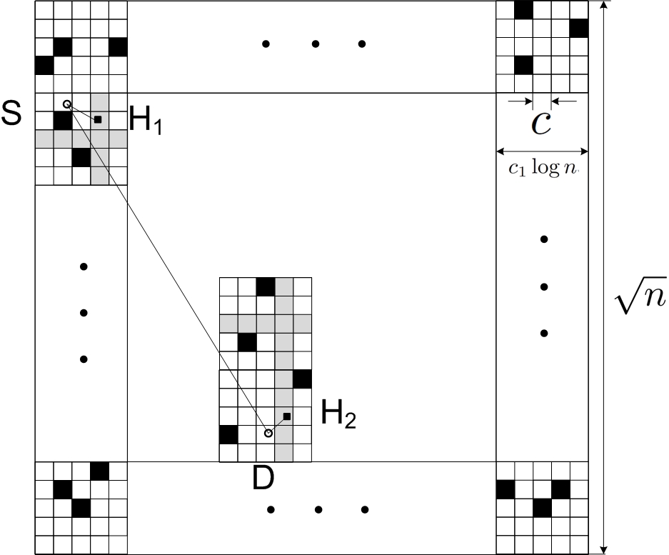
Figure 1: An illustration of partition of $B_{n}$ and the routing algorithm. Black square represents a closed site and white square represents an open site. Grey square represents an open site that forms an open path. $S$ and $D$, indicated by two small hollow circles, are a pair of source and destination nodes. $H_{1}$ and $H_{2}$, indicated by two small black squares, are two nodes located in open sites that form open paths. First $S$ transmits its packets to $H_{1}$ using a transmission range of up to $\sqrt{2}c_{1}\log n$. Then the packets will be routed along the open paths to $H_{2}$, using a transmission range of up to $\sqrt{5}c$. Finally, $H_{2}$ transmits the packets to the destination $D$. If $H_{1}$ itself is a source node, then it transmits its packet directly to the next-hop node along the open path, using a transmission range of up to $\sqrt{5}c$.

IV-A Description of the distributed routing algorithm

We are now ready to explain our routing algorithm. Denote by $SD_{i}$ the line segment connecting node $i$ to its destination. The packets generated by source node $i$ are routed along the squares intersecting $SD_{i}$. A square will only serve the traffic of a source-destination pair if the associated SD line intersects the square. Note that it is trivial to establish that a.a.s. every square has at least one node.

The routing can be divided into three stages:

In the first stage, a source node S, if it is not a node located in an open site that forms one of the open paths, will transmit its packet to a node in a randomly chosen open site that forms an open path. If there are multiple nodes in an open site, a node will be designated randomly to relay all traffic passing through the site. If the source node is already in a site that forms an open path, this stage of routing can be omitted and the routing proceeds directly to the next stage. The maximum distance between the source node and its next-hop node in this stage is bounded by $\sqrt{2}c_{1}\log n$ because the distance between any two nodes located in a square is at most $\sqrt{2}c_{1}\log n$.

In the second stage, the packet will be routed to the adjacent square intersecting the SD line along one of these left-to-right open path or top-to-bottom open paths until the packet reaches a node in the next square. Depending on the location of the open path containing the relay node and the location of the adjacent square, the packet may be routed along a left-to-right open path (when the adjacent square is on the left or on the right of the current square) or along a top-to-bottom open path (when the adjacent square is on the top or on the bottom of the current square). If the packet needs to be switched from a left-to-right open path to a top-to-bottom open path (e.g., when the previous square is on the left of the current square but the next square is on the bottom of the current square), a top-to-bottom open path is chosen randomly from the at least $\omega_{1}\log n$ open path available. The above process continues until the packet reaches the square that contains the destination node. In this stage, the maximum distance between a node and its next-hop node is bounded by $\sqrt{5}c$ because the distance between any two nodes located in two adjacent cells is at most $\sqrt{5}c$.

In the third stage, after reaching the square containing the destination node, if the destination node is located on one of the open paths, the packet will be routed along a multi-hop path to the destination via open paths; if the destination is not located on one of the open paths, the packet will be transmitted to the destination directly and the maximum transmission distance is bounded by $\sqrt{2}c_{1}\log n$.

The same route is used for all packets belonging to the same source-destination pair.

The feasibility of the above routing algorithm is guaranteed by Corollary 2. A node only needs neighborhood information of nodes no more than $\sqrt{5}c_{1}\log n$ away to make a routing decision. The required information for making a proper routing decision is vanishingly small compared with that in the highway algorithm. Furthermore, compared with the network size, the required information is also vanishingly small as $n\rightarrow\infty$. Therefore the routing algorithm can be executed in a distributed manner. On the other hand, we readily acknowledge that neighborhood information of nodes up to $\sqrt{5}c_{1}\log n$ away may be required by the routing algorithm. The required neighborhood information grows logarithmically with the size of the network.

Corollary 3 is a ready consequence of Theorem 1:

Corollary 3.

Let $c=1.7308$ and $c_{1}=3$, a.a.s. there are at least $0.5474\log n$ left-to-right open paths in every horizontal rectangle.

In the rest of this paper, we carry out analysis assuming that $c$ and $c_{1}$ take values specified in Corollary 3 and $\omega_{1}=0.5474$. Fig. 2 shows simulation results of the number of open paths in a horizontal rectangle as the network size $n$ varies. Each random simulation is repeated a large number of times and the average result is shown. The confidence interval is very small and negligible, and thus not plotted in the figure. The lower bound on the number of open paths suggested in Corollary 3 is also plotted for comparison. As shown in Fig. 2, the lower bound is reasonably tight.

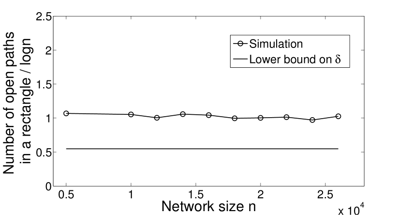
Figure 2: An illustration of the number of left-to-right open paths in a horizontal rectangle as the network size varies. Vertical axis shows the ratio of the number of open paths to $\log n$.

Fig. 3, drawn from a simulation, further gives an intuitive illustration of the open paths in a horizontal rectangle.

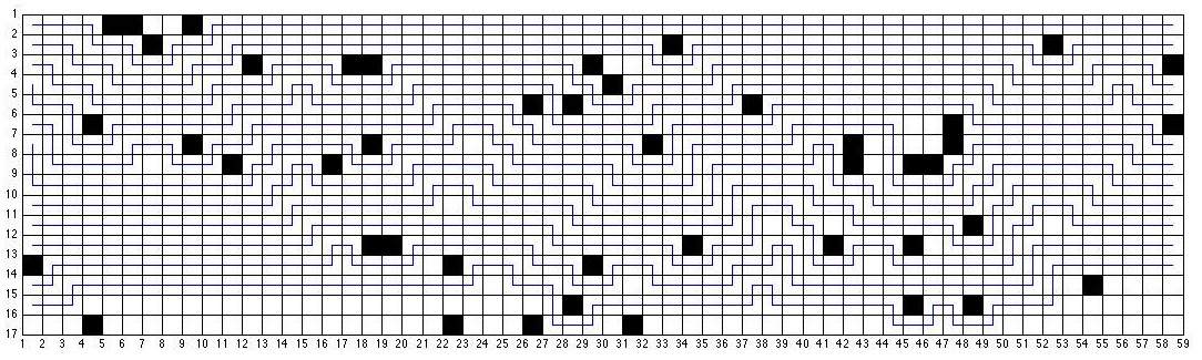
Figure 3: An illustration of left-to-right open paths in a rectangle obtained by computer simulations. Black cells represent closed sites while white cells represent open sites.

After establishing the routing algorithm, next we analyze the traffic load for each node under the algorithm, which forms a key step in analyzing the network capacity.

Lemma 4 shows that the random number of SD lines passing through an arbitrarily chosen square, including the SD lines originating from and ending at the square, is upper bounded.

Lemma 4.

For an arbitrary square in $B_{n}$, the random number of $SD$ lines passing through it, denoted by $Y$, satisfies that

$$\lim_{n\rightarrow\infty}\Pr\left(Y\leq\omega_{2}\sqrt{n}\log n\right)=1$$ (7)

where $\omega_{2}=3.2\left(1+\epsilon\right)\left(1+\delta_{1}\right)c_{1}$, $\epsilon$ and $\delta_{1}$ are arbitrarily small positive constants.

Proof:

See Appendix I. ∎

As a way of establishing the tightness of the bound in Lemma 4, Fig. 4 shows simulation results of the number of SD lines passing a square in comparison with the upper bound in Lemma 4.

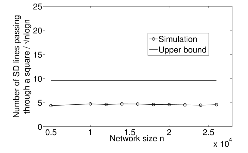
Figure 4: The number of SD lines passing through a square versus the upper bound in Lemma 4. Vertical axis shows the ratio of the number of SD lines passing through a square to $\sqrt{n}\log n$.

Using Corollary 2 and Lemma 4, the following result can be readily established:

Lemma 5.

Each relay node needs to carry the traffic of at most $\frac{\omega_{2}\sqrt{n}}{0.5474}$ source-destination pairs a.a.s.

Note that a node not on an open path does not need to carry the traffic of other source-destination pairs.

V A Solution to the Hidden-node Problem

Our routing algorithm described in the last section needs to use two different transmission ranges of lengths $\Theta\left(1\right)$ and $\Theta\left(\log n\right)$ respectively. The use of two different transmission ranges in CSMA networks will exacerbate the so-called hidden node problem. See Fig. 5 for an illustration. In [1], the problem was addressed by letting nodes operate on two frequency bands, namely, short-range transmissions operate on one frequency band while long-range transmissions operate on the other. Their solution may result in lower spectrum usage because long-range transmission is used less frequently and also poses additional hardware requirements on nodes. Therefore, we present a solution by jointly tuning the transmission power and the carrier-sensing threshold.

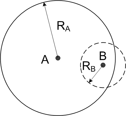
Figure 5: An illustration of the hidden node problem when nodes use different transmission power. Assume that the same carrier-sensing threshold is used by node A and B. The transmission of A using a lager transmission power (node B using a smaller transmission power, respectively) can be detected by nodes located within a distance $R_{A}$ ($R_{B}$, respectively), and $R_{A}>R_{B}$. Consequently B can detect A’s transmission but node A cannot detect node B’s. Therefore even when node B is transmitting, node A still can start its own transmission, thereby resulting in a collision and causing the hidden node problem.

V-A A formal definition of the hidden node problem

Under the SINR model, a set of concurrent transmissions (or links) are said to form an independent set if the SINRs are all above the SINR threshold $\beta$. Let $\mathcal{F}$ be the set of all independent sets. Because of the random and distributed nature of the carrier-sensing operations by individual nodes, the set of simultaneous transmissions observing the carrier-sensing constraint, denoted by $\mathcal{S}^{CS}$, may or may not belong to $\mathcal{F}$, i.e., some transmissions observing the carrier-sensing constraints may still cause the SINRs at some receivers to be above $\beta$. Let $\mathcal{F}^{CS}$ be the set of all $\mathcal{S}^{CS}$s. Let $\Psi$ be the set of concurrent transmissions in a CSMA network. More formally, a hidden node problem is said to occur if $\Psi\in\mathcal{F}^{CS}$ but $\Psi\notin\mathcal{F}$. A CSMA network is said to be hidden node free if its carrier-sensing operations and transmission powers are carefully designed such that all $\Psi\in\mathcal{F}^{CS}$ also meets the condition that $\Psi\in\mathcal{F}$.

For a CSMA network in which uniform transmission power is in use, by setting the carrier-sensing range to be a constant multiple of the transmission range, the hidden node problem can be effectively eliminated [42, 1]. For our routing algorithm using two transmission ranges of lengths $\Theta\left(1\right)$ and $\Theta\left(\log n\right)$ , if the carrier-sensing range is set to be $\Theta\left(\log n\right)$, although the hidden node problem can be eliminated, the number of concurrent transmissions (hence the spatial frequency reuse) will be reduced compared with a carrier-sensing range of $\Theta\left(1\right)$, which in turn causes a reduced capacity. Therefore we manage to have transmissions with different ranges to coexist concurrently instead. In this way, the capacity will be maximized while eliminating the hidden node problem.

More specifically, let $P_{i}$ be the transmission power used for the $i^{th}$ transmission where the same transmitter may use different power when transmitting to different receiver. The transmitter also uses different carrier-sensing threshold when different transmission power is used. Denote by $T_{i}$ the carrier-sensing threshold used for $P_{i}$. Furthermore, let the transmission power of a transmitter be such that the power received at its intended receiver is at least $\bar{P}$ ($\bar{P}$ is a constant not depending on $n$ and the value of $\bar{P}$ will be specified shortly later in this section). The following lemma specifies the relation between $P_{i}$ and $T_{i}$ required for two transmitters to be able to sense each other’s transmission.

Lemma 6.

Let the values of $P_{i}$ and $T_{i}$ be chosen such that the following condition is met

$$P_{i}=\bar{P}T_{i}^{-1}.$$ (8)

For two arbitrary transmitters located at $\boldsymbol{x}_{i}$ and $\boldsymbol{x}_{j}$ respectively, they can sense each other’s transmission iff

$$\left\|\boldsymbol{x}_{i}-\boldsymbol{x}_{j}\right\|<\left(\frac{\bar{P}}{T_{i}T_{j}}\right)^{\frac{1}{\alpha}}=\left(\frac{P_{i}P_{j}}{\bar{P}}\right)^{\frac{1}{\alpha}}$$ (9)

Proof:

When node $i$ located at $\boldsymbol{x}_{i}$ transmits using power $P_{i}$, the power received at node $j$ at location $\boldsymbol{x}_{j}$ is given by $P_{i}\left\|\boldsymbol{x}_{i}-\boldsymbol{x}_{j}\right\|^{-\alpha}$. Let $T_{j}$ be the carrier-sensing threshold of node $j$. The transmission of node $i$ can be detected iff $P_{i}\left\|\boldsymbol{x}_{i}-\boldsymbol{x}_{j}\right\|^{-\alpha}>T_{j}$. Using (8), node $j$ can detect node $i$’s transmission iff $\bar{P}T_{i}^{-1}\left\|\boldsymbol{x}_{i}-\boldsymbol{x}_{j}\right\|^{-\alpha}>T_{j}$ or equivalently $\left\|\boldsymbol{x}_{i}-\boldsymbol{x}_{j}\right\|<\left(\frac{\bar{P}}{T_{i}T_{j}}\right)^{\frac{1}{\alpha}}=\left(\frac{P_{i}P_{j}}{\bar{P}}\right)^{\frac{1}{\alpha}}$. Using a similar argument, node $i$ can detect node $j$’s transmission iff (9) is met. ∎

Lemma 6 shows that by carefully choosing the carrier-sensing threshold according to the transmission power for each transmitter, a major cause of the hidden node problem: a node $A$ senses another node $B$’s transmission but node $B$ cannot sense node $A$’s transmission can be eliminated. In the next several paragraphs, we shall demonstrate how to choose $\bar{P}$, which determines the minimum power received at a receiver, such that the SINR requirement can also be met.

In the first and third stages of our routing algorithm, the maximum distance between a transmitter and a receiver is $\sqrt{2}c_{1}\log n$ while the the maximum distance between a transmitter and a receiver in the second stage is $\sqrt{5}c$. Accordingly, for the first and third stages, we let the transmission power be

$$P^{h}=\bar{P}\left(\sqrt{2}c_{1}\log n\right)^{\alpha}$$ (10)

while for the second stage, the transmission power is set at

$$P^{l}=\bar{P}\left(\sqrt{5}c\right)^{\alpha}$$ (11)

It is trivial to show that the received signal power of all transmissions is at least $\bar{P}$. Furthermore, the following theorem established in our previous work [43, Theorem 1] helps to obtain an upper bound on the interference experienced by any receiver in the network.

Theorem 7.

Consider a CSMA network with nodes distributed arbitrarily on a finite area in $\Re^{2}$ where all nodes transmit at the same power $P$ and use the same carrier-sensing threshold $T$. Furthermore, the power received by a node at $\boldsymbol{x}_{j}$ from a transmitter at $\boldsymbol{x}_{i}$ is given by $P\left\|\boldsymbol{x}_{i}-\boldsymbol{x}_{j}\right\|^{-\alpha}$. Let $r_{0}$ be the distance between a receiver and its transmitter. The maximum interference experienced by the receiver is smaller than or equal to $N_{1}\left(d,r_{0}\right)+N_{2}\left(d\right)$ where

$$N_{1}\left(d,r_{0}\right)= \frac{4\left(\frac{5\sqrt{3}}{4}d-r_{0}\right)^{1-\alpha}\left(\frac{\sqrt{3}}{4}\left(3\alpha-1\right)d-r_{0}\right)}{d^{2}\left(\alpha-1\right)\left(\alpha-2\right)}$$

$$+ \frac{3}{\left(d-r_{0}\right)^{\alpha}}+\frac{3}{\left(\sqrt{3}d-r_{0}\right)^{\alpha}}+\frac{3\left(\frac{3}{2}d-r_{0}\right)^{1-\alpha}}{\left(\alpha-1\right)d}$$ (12)

$$N_{2}\left(d\right) = \frac{3}{d^{\alpha}}+\frac{3(\frac{3}{2})^{1-\alpha}}{\left(\alpha-1\right)d^{\alpha}}+\frac{3}{\left(\sqrt{3}d\right)^{\alpha}}$$ (13)

$$+\frac{3\left(\frac{5}{4}\right)^{1-\alpha}\left(3\alpha-1\right)}{\left(\alpha-1\right)\left(\alpha-2\right)\left(\sqrt{3}d\right)^{\alpha}}$$

and $d=\left(\frac{P}{T}\right)^{\frac{1}{\alpha}}$.

Noting that $N_{1}\left(d,r_{0}\right)$ is a monotonically increasing function of $r_{0}$, it can be readily established using Theorem 7 that in the CSMA network analyzed in this paper in which two sets of transmission powers, carrier-sensing threshold and the maximum transmission range are employed, the maximum interference (for any value of $n$) is bounded by

$$N_{1}\left(\left(\frac{P^{h}}{T^{h}}\right)^{\frac{1}{\alpha}},\sqrt{2}c_{1}\log n\right)+N_{2}\left(\left(\frac{P^{h}}{T^{h}}\right)^{\frac{1}{\alpha}}\right)$$

$$+ N_{1}\left(\left(\frac{P^{l}}{T^{l}}\right)^{\frac{1}{\alpha}},\sqrt{5}c\right)+N_{2}\left(\left(\frac{P^{l}}{T^{l}}\right)^{\frac{1}{\alpha}}\right)$$ (14)

where $T^{l}$ and $T^{h}$ are the carrier-sensing threshold chosen for $P^{l}$ and $P^{h}$ respectively according to (8).

Remark 8.

At the expense of more analytical efforts, a tighter bound on interference can be established that the maximum interference in the CSMA network considered in this paper is bounded by $N_{1}\left(\left(\frac{P^{l}}{T^{l}}\right)^{\frac{1}{\alpha}},\sqrt{5}c\right)+N_{2}\left(\left(\frac{P^{l}}{T^{l}}\right)^{\frac{1}{\alpha}}\right)$ for any value of $n$. Because for a sufficiently large network, which is the focus of this paper, the difference between this bound and the upper bound in (14) is negligibly small, we choose to omit the analysis due to space limitation.

Noting that $\left(\frac{P^{h}}{T^{h}}\right)^{\frac{1}{\alpha}}=\bar{P}^{\frac{1}{\alpha}}\left(\sqrt{2}c_{1}\log n\right)^{2}$, $\left(\frac{P^{l}}{T^{l}}\right)^{\frac{1}{\alpha}}=\bar{P}^{\frac{1}{\alpha}}\left(\sqrt{5}c\right)^{2}$ and $d=\left(\frac{P}{T}\right)^{\frac{1}{\alpha}}$, it is easy to conclude using (12) and (13) that when $\alpha>1$, the contribution of the first two terms $N_{1}\left(\left(\frac{P^{h}}{T^{h}}\right)^{\frac{1}{\alpha}},\sqrt{2}c_{1}\log n\right)+N_{2}\left(\left(\frac{P^{h}}{T^{h}}\right)^{\frac{1}{\alpha}}\right)$, attributable to transmissions using a larger transmission power, become vanishingly small compared with the last two terms as $n\rightarrow\infty$. The following theorem provides guidance on how to choose $\bar{P}$ to meet the SINR requirements for all concurrent transmissions in a large CSMA network.

Theorem 9.

For an arbitrarily high SINR requirement $\beta$, there exists a value of $\bar{P}$ for sufficiently large $n$ such that the SINR of all transmissions in a CSMA network, in which each transmitter sets its transmission power and carrier sensing threshold according to the relationship in Lemma 6, is greater than or equal to $\beta$. Furthermore, the value of $\bar{P}$ is given implicitly by the following equation

$$\frac{\bar{P}}{N_{1}\left(\left(\frac{P^{l}}{T^{l}}\right)^{\frac{1}{\alpha}},\sqrt{5}c\right)+N_{2}\left(\left(\frac{P^{l}}{T^{l}}\right)^{\frac{1}{\alpha}}\right)}=\beta$$ (15)

Proof:

Noting that the minimum received power is $\bar{P}$, the theorem becomes an easy consequence of the interference upper bound established earlier in the section. ∎

As a brief summary of the results of this section, Theorem 9 gives guidance on how to choose $\bar{P}$ to meet the SINR requirement. More specifically, noting that $\left(\frac{P^{l}}{T^{l}}\right)^{\frac{1}{\alpha}}=\bar{P}^{\frac{1}{\alpha}}\left(\sqrt{5}c\right)^{2}$ and using equations (12) and (13), equation (15) becomes an implicit equation of $\bar{P}$. Solving the equation, the value of $\bar{P}$ that meets the SINR requirement can be obtained, which is independent of $n$. Given the value of $\bar{P}$, the other parameters in the CSMA network, i.e. $P^{h}$, $P^{l}$ and the carrier sensing thresholds, can all be determined using equations (8), (10) and (11) respectively. It can be readily established using the analysis presented in this section that the CSMA network whose transmission power and carrier sensing threshold are chosen following the above steps are immune from the hidden node problem.

VI Back Off Timer Setting and Capacity Analysis

In the last section, we demonstrated how to choose the transmission power and the carrier sensing threshold to solve the hidden node problem. In the CSMA network in which nodes may use two different transmission powers, a potential problem that may arise is that nodes using the larger transmission power may potentially contend with more nodes for transmission opportunities. Therefore nodes using the larger transmission power may not get a fair transmission opportunity compared with nodes using the smaller transmission power. This may potentially causes nodes using the larger transmission power to become a bottleneck in throughput which reduces the overall network capacity. In this section, we demonstrate how to choose another controllable parameter in CSMA protocols, i.e., back off timer, to conquer the difficulty.

Same as that in references [1] and [44], we consider a CSMA protocol in which the initial back off timer is a random variable following an exponential distribution. Nodes using different transmission power may however choose different mean value to use in the exponential distribution governing their respective random initial back off timer. The following theorem provides the basis for choosing these mean values.

Theorem 10.

Let $\delta_{2}$ and $\delta_{3}$ be two small positive constants. If transmissions using a low transmit power $P^{l}$ set their initial back off time to be exponentially distributed with mean $\lambda_{l}=1$ and transmissions using a high transmission power $P^{h}$ set their initial back off time to be exponentially distributed with mean $\lambda_{h}=\frac{1}{\log^{2}n}$, then

(i) a.a.s. each low power transmission can be active with a constant probability greater than or equal to

$$\omega_{3}=\frac{1}{\pi\left(5\bar{P}^{\frac{1}{\alpha}}c\right)^{2}+\left(1+\delta_{2}\right)10\pi c^{2}c_{1}^{2}\bar{P}^{\frac{2}{\alpha}}+1}$$ (16)

(ii) a.a.s. each high power transmission can be active with a probability greater than or equal to

$$\omega_{4}=\frac{1}{\pi\left(\sqrt{10}c_{1}\bar{P}^{\frac{1}{\alpha}}\right)^{2}\log^{4}n+\left(1+\delta_{3}\right)4\pi c_{1}^{4}\bar{P}^{\frac{2}{\alpha}}\log^{4}n+1}$$

Proof:

See Appendix II. ∎

Fig. 6 shows the transmission opportunity (or the medium access probability) of a node using $P^{l}$ versus the lower bound in Theorem 10 for different values of $n$.

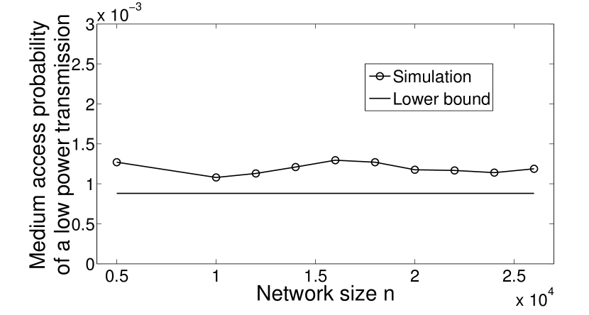
Figure 6: A comparison between the simulation result on the medium access probability of a node using the low power transmission with the lower bound in Theorem 10 where $\beta=10$ and $\alpha=4$.

On the basis of the results established in this section and in the earlier sections, we present the following theorem which forms the major result of this paper.

Theorem 11.

The achievable per-node throughput in the CSMA network is greater than or equal to

$$\frac{0.5474\omega_{3}}{\omega_{2}\sqrt{n}}W;$$ (17)

and is smaller than or equal to

$$\frac{1}{0.52c\left(5\pi c^{2}c_{1}^{2}\bar{P}^{\frac{2}{\alpha}}+1\right)\sqrt{n}}\times W$$

a.a.s. as $n\rightarrow\infty$, where $\omega_{2}$ is given in Lemma 4 and $\omega_{3}$ is given by (16).

Proof:

We first show that the achievable per-node throughput is lower bounded by $\frac{0.5474\omega_{3}}{\omega_{2}\sqrt{n}}W$. Let $\lambda_{1}\left(n\right)$ ($\lambda_{2}\left(n\right)$, respectively) be the per-node throughput that can be achieved in the first and the third (the second, respectively) stages of our routing algorithm. Obviously the final per-node throughput $\lambda\left(n\right)$ satisfies $\lambda\left(n\right)=\min\left\{\lambda_{1}\left(n\right),\lambda_{2}\left(n\right)\right\}$. In the following, we analyze $\lambda_{1}\left(n\right)$ and $\lambda_{2}\left(n\right)$ separately.

As an easy consequence of Lemma 5, a.a.s. each relay node carries the traffic of at most $\frac{\omega_{2}\sqrt{n}}{0.5474}$ source-destination pairs. According to the first statement of Theorem 10, a.a.s. each relay node on an open path can access the channel with a probability of at least $\omega_{3}$, which is a constant independent of $n$. The conclusion then readily follows that $\lim_{n\rightarrow\infty}\Pr\left(\lambda_{2}\left(n\right)\geq\frac{0.5474\omega_{3}}{\omega_{2}\sqrt{n}}W\right)=1$.

For the second stage of the routing, note that a source or a destination node not on an open path does not need to carry traffic for other source-destination pairs. Using the second statement of Theorem 10, conclusion follows that $\lambda_{1}\left(n\right)=\Omega\left(\frac{1}{\log^{4}n}\right)$.

Combining the above two results on $\lambda_{1}\left(n\right)$ and $\lambda_{2}\left(n\right)$ and noting that the capacity bottleneck lies in the second stage, the first statement in this theorem is proved.

We now further show that the achievable per-node throughput is upper bounded by $\frac{W}{0.52c\left(5\pi c^{2}c_{1}^{2}\bar{P}^{\frac{2}{\alpha}}+1\right)\sqrt{n}}$. The upper bound is to be established using a result proved in our previous work [45, Corollary 6], which shows that the per-node throughput is equal to the product of the average number of simultaneous transmissions and the link capacity divided by the product of the average number of transmissions required to deliver a packet to its destination and the number of source-destination pairs. We first analyze the average number of transmissions required for a packet to reach its destination. The average distance between a randomly chosen source-destination pair is $0.52\sqrt{n}$ [46]. A packet moves by one cell in each hop on an open path where the contribution of the last mile transmission between a source (a destination) and an open-path node is vanishingly small compared with $0.52\sqrt{n}$. Thus a.a.s. the average number of hops traversed by a packet is at least $\frac{0.52\sqrt{n}}{c}$. Next we analyze the average number of simultaneous transmissions. Since there is at most one node in a cell acting as an open path node, there are at most $\frac{n}{c^{2}}$ open path nodes in the network. Following the same procedure in obtaining (23), (24) and (25), we have that $\Pr\left[\eta_{i}^{l}\right]\leq\frac{1}{5\pi c^{2}c_{1}^{2}\bar{P}^{\frac{2}{\alpha}}+1}$. Therefore, the average number of simultaneous transmissions is at most $\frac{n}{c^{2}}\times\frac{1}{5\pi c^{2}c_{1}^{2}\bar{P}^{\frac{2}{\alpha}}+1}$ (Note that when a non-open-path node transmits using $P^{h}$, the number of simultaneous transmissions will only reduce). As a ready consequence of the above analysis and [45, Corollary 6], an upper bound on the per-node throughput results. ∎

The lower bound on the per-node throughput provided in Theorem 11 is order optimal in the sense that the throughput is of the same order as the known result on the optimum per-node throughput [4] of networks under the same settings. Furthermore, Theorem 11 gives the pre-constant preceding the order of the per-node throughput: $\frac{0.5474\omega_{3}}{\omega_{2}}$. A detail examination of the pre-constant reveals that the pre-constant can be separated into the product of two terms: $\frac{0.5474}{\omega_{2}}$ and $\omega_{3}$. The first term $\frac{0.5474}{\omega_{2}}$ is entirely determined by the routing algorithm, more specifically determined by how the routing algorithm distribute traffic load among relay nodes and among source-destination pairs. The second term $\omega_{3}$ is entirely determined by the scheduling algorithm and some physical layer details, i.e., the SINR requirement, interference and propagation model. The above observation appears to suggest that impact of the routing algorithm and the scheduling algorithm can be decoupled and studied separately, and the two algorithms that determine the overall network capacity can be optimized separately.

Fig. 7 shows a comparison of the per-node throughput obtained from simulations, the upper lower bounds obtained in Theorem 11 for different values of $n$. To facilitate comparison, Fig. 8 further shows the ratio of the per-node throughput obtained from simulations to the throughput lower bound and the ratio of the throughput upper bound to the throughput lower bound. As shown in the figures, the lower bound is fairly tight and the upper bound is also within a factor of $10$ of the simulation result. The simulation results demonstrate that the pre-constant obtained in our study provides a pretty accurate characterization of the per-node throughput.

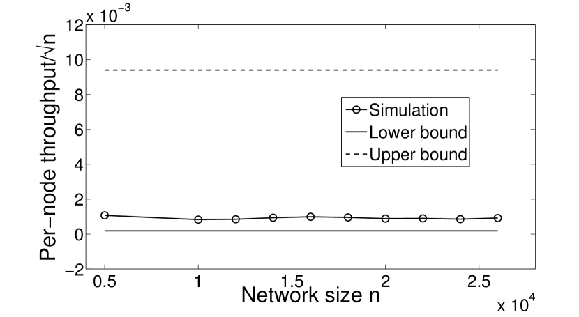
Figure 7: A simulation of per-node throughput with $\alpha=4$ and $\beta=10$. For comparison, the upper and the lower bound obtained in the paper is also shown.

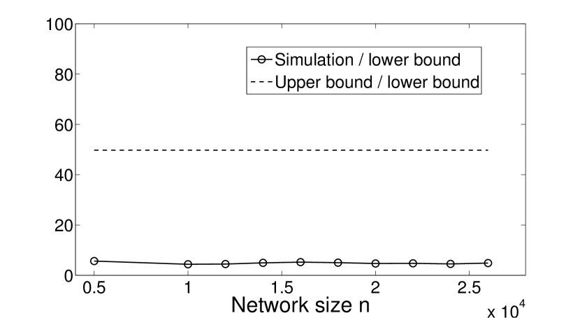
Figure 8: A simulation of per-node throughput with $\alpha=4$ and $\beta=10$. For comparison, the upper and the lower bound obtained in the paper are also shown. To facilitate comparison, both the per-node throughput obtained from simulations and the per-node throughput upper bound are normalized by the per-node throughput lower bound.

VII Conclusion

In this paper, we studied the transport capacity of large wireless multi-hop CSMA networks. We showed that by carefully choosing the controllable parameters in the CSMA protocol and designing the routing algorithm, a network running distributed CSMA scheduling algorithm and each node making routing decisions based on local information only can also achieve an order-optimal throughput of $\Theta\left(\frac{1}{\sqrt{n}}\right)$, which is the same as that of large networks employing centralized routing and scheduling algorithms. Furthermore, we not only gave the order of the throughput but also derived the pre-constant preceding the order by giving an upper and a lower bound of the transport capacity. The tightness of the bounds was validated using simulations. Theoretical analysis was presented on tuning the carrier-sensing threshold and the transmission power to avoid hidden node problems and on tuning the back off timer distribution to ensure each node gain a fair access to the channel in CSMA networks using non-uniform transmission powers. The principle developed through the analysis was expected to be also helpful to set the corresponding parameters of CSMA networks in a more realistic setting.

Appendix I Proof of Lemma 4

In the proof of Lemma 4, we will make use of a result established in the stochastic ordering theory [47]. For two real valued random variables $X_{1}$ and $X_{2}$, we say $X_{1}\leq_{st}X_{2}$ iff for all $x\in\left(-\infty,\infty\right)$, $\Pr\left(X_{1}>x\right)\leq\Pr\left(X_{2}>x\right)$.

Theorem 12.

[47, Theorem 1(a)]Suppose $X_{i}$ follows a Binomial distribution with parameters $n_{i}\in\mathbb{N}$ and $p_{i}\in\left(0,1\right)$, denote the distribution of $X_{i}$ by $B\left(n_{i},p_{i}\right)$, $i=1,2$, i.e., $X_{i}\sim B\left(n_{i},p_{i}\right)$. We have $X_{1}\leq_{st}X_{2}$ iff $\left(1-p_{1}\right)^{n_{1}}\geq\left(1-p_{2}\right)^{n_{2}}$ and $n_{1}\leq n_{2}$.

As an easy consequence of the above theorem, for three independent Binomial random variables $X_{1}\sim B\left(n_{1},p_{1}\right)$, $X_{2}\sim B\left(n_{1},p_{2}\right)$ and $X_{3}\sim B\left(n_{2},p_{2}\right)$ with $n_{1}\leq n_{2}$ and $p_{1}\leq p_{2}$, it can be concluded that $X_{1}\leq_{st}X_{2}\leq_{st}X_{3}$.

Now we are ready to prove Lemma 4. Let $Y_{i}^{j}$ be the indicator random variable for the event that the $SD_{i}$ passes through the $j^{th}$ square:

$$Y_{i}^{j}=\begin{cases}1&\textrm{if $SD_{i}$passes through the $j$th square}\\ 0&\textrm{otherwise.}\end{cases}$$

We shall derive an upper bound on $\Pr\left[Y_{i}^{j}=1\right]$ for any $j\in\left[1,\,\frac{n}{\log^{2}n}\right]$. Circumscribe the $j^{th}$ square with a small circle of radius $\frac{\sqrt{2}}{2}c_{1}\log n$, as shown in Fig. 9. For a source $S$ located outside the square and at a distance $x$ from the center of the square, the angle $\theta\left(x\right)$ subtended by the circle at S is $\theta\left(x\right)=2\arcsin\frac{\frac{\sqrt{2}}{2}c_{1}\log n}{x}$. Using the fact that $\arcsin x\leq 1.6x$ when $0\leq x\leq 1$, we have

$$\theta\left(x\right)=1.6\arcsin\frac{\frac{\sqrt{2}}{2}c_{1}\log n}{x}\leq 3.2\frac{\frac{\sqrt{2}}{2}c_{1}\log n}{x}$$ (18)

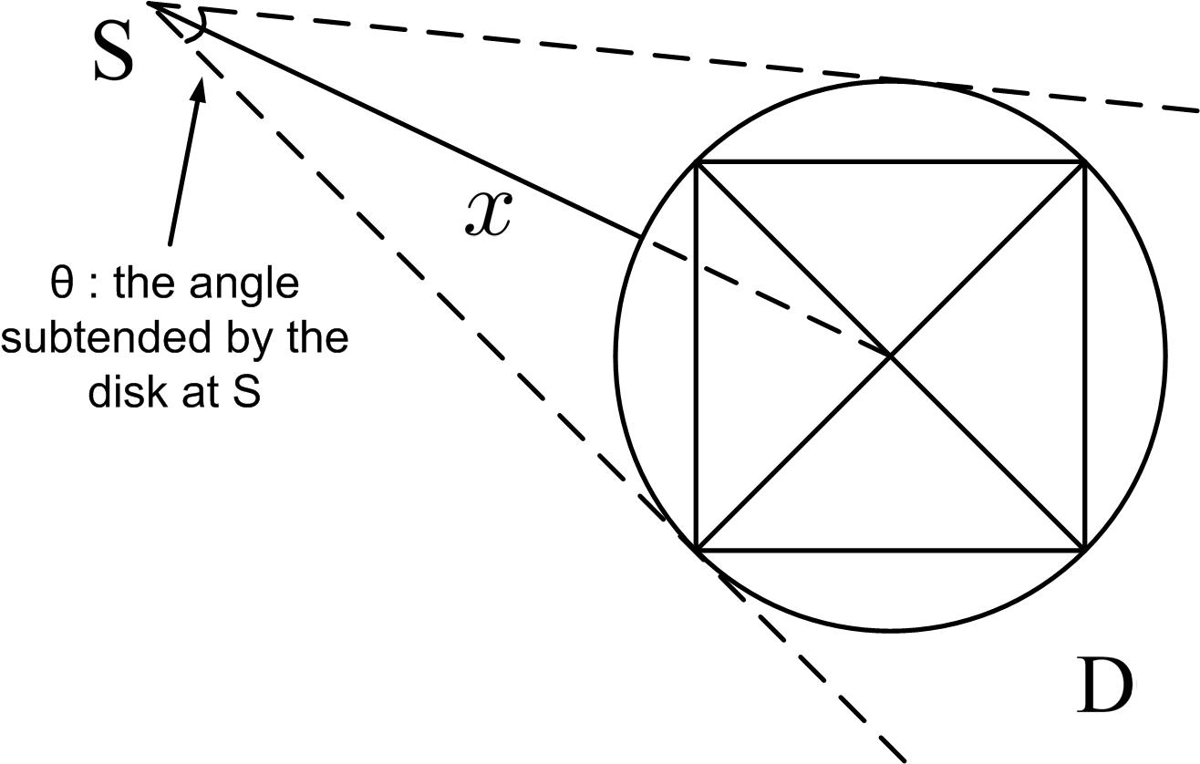
Figure 9: An illustration of a SD line intersecting the circumscribed circle

Noting that $B_{n}$ is of size $\sqrt{n}\times\sqrt{n}$, the area of the sector formed by the two dashed tangents Fig. 9 and the boarder of $B_{n}$ is at most $\frac{\theta\left(x\right)}{2\pi}n$. If the destination of $S$, denoted by $D$, does not lie in this sector, then the associated $SD$ line does not pass through the circle. Therefore, the probability that the $SD$ line intersecting the circle is at most $\frac{\theta\left(x\right)}{2\pi}$. Considering that the circle is located in a $\sqrt{n}\times\sqrt{n}$ box $B_{n}$, the probability density that $S$ is at a distance $x$ from the circle can be shown to be upper bounded by $\frac{2\pi x}{n}$. It follows from the above analysis and (18) that

$$\Pr\left[Y_{i}^{j}=1\right]$$

$$\leq \int_{0}^{\sqrt{2n}}\frac{3.2\times\frac{\sqrt{2}}{2}c_{1}\log n}{2\pi x}\times\frac{2\pi x}{n}\mathrm{d}x=\frac{3.2c_{1}\log n}{\sqrt{n}}$$ (19)

Recall that $\Gamma$ represents the set of indices of all nodes in the network. For a fixed square $j$, the total number of $SD$ lines passing through it is given by $Y^{j}=\sum_{i=1}^{\left|\Gamma\right|}Y_{i}^{j}$, which is the sum of i.i.d. Bernoulli random variables since the locations of nodes are independent and $Y_{i}^{j}$ depends only on the locations of source and destination nodes of the $i^{th}$ source-destination pair. Therefore $Y^{j}$ follows the Binomial distribution, i.e., $Y^{j}\sim B\left(\left|\Gamma\right|,\,\Pr\left[Y_{i}^{j}=1\right]\right)$. As an easy consequence of the Poisson distribution of nodes, a.a.s. the total number of nodes $\left|\Gamma\right|\leq\left(1+\epsilon\right)n$, where $\epsilon$ is an arbitrarily small positive constant. Define another Binomial random variable $\tilde{Y}^{j}\sim B\left(\left(1+\epsilon\right)n,\frac{4c_{1}\log n}{\sqrt{n}}\right)$ . It follows from Theorem 12 that

$$Y^{j}\leq_{\textrm{st}}\tilde{Y}^{j}$$

It can be further shown that for any $0<\delta_{1}<1$,

$$\Pr\left[Y^{j}>\left(1+\delta_{1}\right)\left(1+\epsilon\right)n\frac{3.2c_{1}\log n}{\sqrt{n}}\right]$$ (20)

$$\leq \Pr\left[\tilde{Y}^{j}>\left(1+\delta_{1}\right)\left(1+\epsilon\right)n\frac{3.2c_{1}\log n}{\sqrt{n}}\right]$$

$$= \Pr\left[\tilde{Y}^{j}>\left(1+\delta_{1}\right)\textrm{E}\left[\tilde{Y}^{j}\right]\right]$$

$$\leq \exp\left(-\frac{\delta_{1}^{2}}{3}\textrm{E}\left[\tilde{Y}^{j}\right]\right)$$

$$= \exp\left(-\frac{3.2\left(1+\epsilon\right)\delta_{1}^{2}c_{1}\sqrt{n}\log n}{3}\right)$$ (21)

where (20) results from the Chernoff bound. Using the union bound and the above result, we have

$$\Pr\left[\bigcup_{j=1}^{\frac{n}{c_{1}^{2}\log^{2}n}}Y^{j}>3.2\left(1+\epsilon\right)\left(1+\delta_{1}\right)c_{1}\sqrt{n}\log n\right]$$ (22)

$$\leq \frac{n}{c_{1}^{2}\log^{2}n}\exp\left(-\frac{3.2\left(1+\epsilon\right)\delta_{1}^{2}c_{1}\sqrt{n}\log n}{3}\right)$$

Noting that $\frac{n}{c_{1}^{2}\log^{2}n}\exp\left(-\frac{3.2\left(1+\epsilon\right)\delta_{1}^{2}c_{1}\sqrt{n}\log n}{3}\right)\rightarrow 0$ as $n\rightarrow\infty$, therefore a.a.s. $Y^{j}\leq 3.2\left(1+\epsilon\right)\left(1+\delta_{1}\right)c_{1}\sqrt{n}\log n$ for any $j\in\left[1,\,\frac{n}{\log^{2}n}\right]$ which completes the proof of Lemma 4.

Appendix II Proof of Theorem 10

Consider a node $i$ on an open path located at $\boldsymbol{x}_{i}$ transmitting with power $P^{l}=\bar{P}\left(\sqrt{5}c\right)^{\alpha}$. Since the highest transmission power used in the network is $P^{h}=\bar{P}\left(\sqrt{2}c_{1}\log n\right)^{\alpha}$, by (9), the furtherest transmitter that node $i$ can sense is within a distance of $\sqrt{10}cc_{1}\bar{P}^{\frac{1}{\alpha}}\log n$. Denote by $\mathcal{D}\left(\boldsymbol{x},\,r\right)$ a disk centered at $\boldsymbol{x}$ and with a radius of $r$. All nodes that are possibly competing with node $i$ for transmission opportunities are located within $\mathcal{D}\left(\boldsymbol{x}_{i},\,\sqrt{10}cc_{1}\bar{P}^{\frac{1}{\alpha}}\log n\right)$. Denote by $\mathcal{A}\left(\boldsymbol{x},\,r_{1},\,r_{2}\right)$ an annulus area centered at $\boldsymbol{x}$ with an inner radius $r_{1}$ and an outer radius $r_{2}$. A little reflection shows that all nodes using the low transmission power $P^{l}$ and competing with node $i$ must be located in $\mathcal{D}\left(\boldsymbol{x}_{i},\,5\bar{P}^{\frac{1}{\alpha}}c^{2}\right)$, and the nodes in $\mathcal{A}\left(\boldsymbol{x}_{i},\,5\bar{P}^{\frac{1}{\alpha}}c^{2},\,\sqrt{10}cc_{1}\bar{P}^{\frac{1}{\alpha}}\log n\right)$ that compete with node $\boldsymbol{x}_{i}$ must use the high transmit power $P^{h}$. Note that in each open site that forms the open path, only one node serves as the relay node. Hence, there are at most $\frac{\pi\left(5\bar{P}^{\frac{1}{\alpha}}c^{2}\right)^{2}}{c^{2}}=\pi\left(5\bar{P}^{\frac{1}{\alpha}}c\right)^{2}$ open path nodes in $\mathcal{D}\left(\boldsymbol{x}_{i},\,5\bar{P}^{\frac{1}{\alpha}}c^{2}\right)$ that use $P^{l}$. Let $\mathcal{N}\left(\boldsymbol{x},\,r\right)$ be the random number of nodes located in $\mathcal{D}\left(\boldsymbol{x},\,r\right)$. Next we provide an asymptotic upper bound on the number of nodes in $\mathcal{D}\left(\boldsymbol{x}_{i},\,\sqrt{10}cc_{1}\bar{P}^{\frac{1}{\alpha}}\log n\right)$ for any node $i$ on an open path. Denoting by $\mathcal{H}$ the set of indices of nodes on open paths, clearly $\left|\mathcal{H}\right|<\frac{n}{c^{2}}$. By Chernoff bound and the union bound, we have for an arbitrarily small positive constant $\delta_{2}$,

$$\Pr\left[\bigcup_{i\in\mathcal{H}}\mathcal{N}\left(\boldsymbol{x}_{i},\sqrt{10}cc_{1}\bar{P}^{\frac{1}{\alpha}}\log n\right)\geq\right.$$ (23)

$$\left.\left(1+\delta_{2}\right)10\pi c^{2}c_{1}^{2}\bar{P}^{\frac{2}{\alpha}}\log^{2}n\right]$$

$$= \Pr\left[\bigcup_{i\in\mathcal{H}}\mathcal{N}\left(\boldsymbol{x}_{i},\,\sqrt{10}cc_{1}\bar{P}^{\frac{1}{\alpha}}\log n\right)\geq\right.$$

$$\left.\left(1+\delta_{2}\right)\textrm{E}\left[\mathcal{N}\left(\boldsymbol{x}_{i},\,\sqrt{10}cc_{1}\bar{P}^{\frac{1}{\alpha}}\log n\right)\right]\right]$$

$$\leq \frac{n}{c^{2}}e^{-\frac{\delta_{2}^{2}}{3}\textrm{E}\left[\mathcal{N}\left(\boldsymbol{x}_{i},\,\sqrt{10}cc_{1}\bar{P}^{\frac{1}{\alpha}}\log n\right)\right]}$$

where $E$ denotes the expectation operator. It can be readily shown that $\frac{n}{c^{2}}\exp\left\{-\frac{\delta_{2}^{2}}{3}\textrm{E}\left[\mathcal{N}\left(\boldsymbol{x}_{i},\,\sqrt{10}cc_{1}\bar{P}^{\frac{1}{\alpha}}\log n\right)\right]\right\}$ approaches $0$ as $n\rightarrow\infty$. Therefore a.a.s. the number of nodes within a distance $\sqrt{10}cc_{1}\bar{P}^{\frac{1}{\alpha}}\log n$ of an open path node is bounded above by $\left(1+\delta_{2}\right)10\pi c^{2}c_{1}^{2}\bar{P}^{\frac{2}{\alpha}}\log^{2}n$.

Next we analyze the transmission opportunity of an open path node. Denote by $t_{i}$ the back off timer of node $i$ at a particular time instant when the channel is idle. Denote by $\mathcal{C}_{i}$ the set of indices of nodes that compete with node $i$ for transmission. Following the CSMA protocol, node $i$ can become an active transmitter in the competition if

$$t_{i}<\min_{j\in\mathcal{C}_{i}\backslash\left\{i\right\}}t_{j}.$$

Let $\eta_{i}^{l}$ be the event that a transmission of node $i$ using the low transmit power is active. Using the “memoryless” property of an exponential distribution that for a timer following an exponential distribution, the amount of lapsed time does not alter the distribution of the remaining value of the timer, it can be shown that for any $i\in\mathcal{H}$

$$\Pr\left[\eta_{i}^{l}\right]$$ (24)

$$= \Pr\left[t_{i}<\min_{j\in\mathcal{C}_{i}\backslash\left\{i\right\}}t_{j}\right]$$

$$\geq \int_{0}^{\infty}\left(e^{-\lambda_{l}t}\right)^{\pi\left(5\bar{P}^{\frac{1}{\alpha}}c\right)^{2}}\left(e^{-\lambda_{h}t}\right)^{\left(1+\delta_{2}\right)10\pi c^{2}c_{1}^{2}\bar{P}^{\frac{2}{\alpha}}\log^{2}n}$$

$$\times\lambda_{l}e^{-\lambda_{l}t}\mathrm{d}t$$

where in the above equation the term $\left(e^{-\lambda_{l}t}\right)^{\pi\left(5\bar{P}^{\frac{1}{\alpha}}c\right)^{2}}$ represents the probability that at a randomly chosen time instant when the channel is idle, all $\pi\left(5\bar{P}^{\frac{1}{\alpha}}c\right)^{2}$ open path nodes in $\mathcal{D}\left(\boldsymbol{x}_{i},\,5\bar{P}^{\frac{1}{\alpha}}c^{2}\right)$, which are competing for transmission opportunities with node $i$, have their respective back off timer larger than a particular value $t$; the term $\left(e^{-\lambda_{h}t}\right)^{\left(1+\delta_{2}\right)10\pi c^{2}c_{1}^{2}\bar{P}^{\frac{2}{\alpha}}\log^{2}n}$ represents the probability that all nodes using $P^{h}$ in $\mathcal{D}\left(\boldsymbol{x}_{i},\,\sqrt{10}cc_{1}\bar{P}^{\frac{1}{\alpha}}\log n\right)$, which are competing for transmission opportunities with node $i$, have their respective back off timer larger than $t$; the term $\lambda_{l}e^{-\lambda_{l}t}$ is the pdf of the back off timer of node $i$. It can be further shown from (24) that for any $i\in\mathcal{H}$,

$$\Pr\left[\eta_{i}^{l}\right]$$ (25)

$$\geq \lambda_{l}\int_{0}^{\infty}e^{-\left(\pi\left(5\bar{P}^{\frac{1}{\alpha}}c\right)^{2}\lambda_{l}+\lambda_{h}\left(1+\delta_{2}\right)10\pi c^{2}c_{1}^{2}\bar{P}^{\frac{2}{\alpha}}\log^{2}n+\lambda_{l}\right)t}\mathrm{d}t$$

$$= \frac{\lambda_{l}}{\pi\left(5\bar{P}^{\frac{1}{\alpha}}c\right)^{2}\lambda_{l}+\lambda_{h}\left(1+\delta_{2}\right)10\pi c^{2}c_{1}^{2}\bar{P}^{\frac{2}{\alpha}}\log^{2}n+\lambda_{l}}$$

$$= \frac{1}{\pi\left(5\bar{P}^{\frac{1}{\alpha}}c\right)^{2}+\frac{\lambda_{h}}{\lambda_{l}}\left(1+\delta_{2}\right)10\pi c^{2}c_{1}^{2}\bar{P}^{\frac{2}{\alpha}}\log^{2}n+1}$$

$$= \frac{1}{\pi\left(5\bar{P}^{\frac{1}{\alpha}}c\right)^{2}+\left(1+\delta_{2}\right)10\pi c^{2}c_{1}^{2}\bar{P}^{\frac{2}{\alpha}}+1}.$$

Now we continue to prove the second part of Theorem 10. Consider that a node $j$ transmits using the high power $P^{h}=\bar{P}\left(\sqrt{2}c_{1}\log n\right)^{\alpha}$. By (9), all nodes that are possibly competing with node $j$ are located within $\mathcal{D}\left(\boldsymbol{x}_{j},\,2c_{1}^{2}\bar{P}^{\frac{1}{\alpha}}\log^{2}n\right)$. Furthermore, among the nodes competing with node $j$, those open path nodes using the lower transmission power $P^{l}$ must be located in $\mathcal{D}\left(\boldsymbol{x}_{j},\,\sqrt{10}cc_{1}\bar{P}^{\frac{1}{\alpha}}\log n\right)$, and the number of these open path nodes is at most $\frac{\pi\left(\sqrt{10}cc_{1}\bar{P}^{\frac{1}{\alpha}}\log n\right)^{2}}{c^{2}}=\pi\left(\sqrt{10}c_{1}\bar{P}^{\frac{1}{\alpha}}\log n\right)^{2}$. Next we derive an upper bound on the number of nodes in $\mathcal{D}\left(\boldsymbol{x}_{j},\,2c_{1}^{2}\bar{P}^{\frac{1}{\alpha}}\log^{2}n\right)$ competing with node $j$ for any $j\in\mathcal{O}$ where $\mathcal{O}$ is the set of indices of nodes using the high power. It can be easily shown that $\lim_{n\rightarrow\infty}\Pr\left(\left|\mathcal{O}\right|<2n\right)=1$. Using the union bound and the Chernoff bound, we have for any small positive constant $\delta_{3}$,

$$\Pr\left[\bigcup_{j\in\mathcal{O}}\mathcal{N}\left(\boldsymbol{x}_{j},2c_{1}^{2}\bar{P}^{\frac{1}{\alpha}}\log^{2}n\right)\geq\right.$$

$$\left.\left(1+\delta_{3}\right)4\pi c_{1}^{4}\bar{P}^{\frac{2}{\alpha}}\log^{4}n\right]$$

$$= \Pr\left[\bigcup_{j\in\mathcal{O}}\mathcal{N}\left(\boldsymbol{x}_{j},2c_{1}^{2}\bar{P}^{\frac{1}{\alpha}}\log^{2}n\right)\geq\right.$$

$$\left.\left(1+\delta_{3}\right)\textrm{E}\left[\mathcal{N}\left(\boldsymbol{x}_{j},2c_{1}^{2}\bar{P}^{\frac{1}{\alpha}}\log^{2}n\right)\right]\right]$$

$$\leq 2ne^{-\frac{\delta_{3}^{2}}{3}\textrm{E}\left[\mathcal{N}\left(\boldsymbol{x}_{j},\,2c_{1}^{2}\bar{P}^{\frac{1}{\alpha}}\log^{2}n\right)\right]}$$

Obviously $2n\exp\left\{-\frac{\delta_{3}^{2}}{3}\textrm{E}\left[\mathcal{N}\left(\boldsymbol{x}_{j},\,2c_{1}^{2}\bar{P}^{\frac{1}{\alpha}}\log^{2}n\right)\right]\right\}$ approaches $0$ as $n\rightarrow\infty$. Therefore a.a.s. the number of nodes competing with node $j$ where $j\in\mathcal{O}$ is smaller than or equal to $\left(1+\delta_{3}\right)4\pi c_{1}^{4}\bar{P}^{\frac{2}{\alpha}}\log^{4}n$. Let $\eta_{j}^{h}$ be the event that node $j$, $j\in\mathcal{O}$, is active. It can be shown that for any $j\in\mathcal{O}$,

$$\Pr\left[\eta_{j}^{h}\right]$$

$$\geq \int_{0}^{\infty}\left(e^{-\lambda_{l}t}\right)^{\pi\left(\sqrt{10}c_{1}\bar{P}^{\frac{1}{\alpha}}\log n\right)^{2}}\left(e^{-\lambda_{h}t}\right)^{\left(1+\delta_{3}\right)4\pi c_{1}^{4}\bar{P}^{\frac{2}{\alpha}}\log^{4}n}$$

$$\times\lambda_{h}e^{-\lambda_{h}t}\mathrm{d}t$$

$$= \frac{1}{\pi\left(\sqrt{10}c_{1}\bar{P}^{\frac{1}{\alpha}}\log n\right)^{2}\frac{\lambda_{l}}{\lambda_{h}}+1\left(1+\delta_{3}\right)4\pi c_{1}^{4}\bar{P}^{\frac{2}{\alpha}}\log^{4}n+1}$$

$$= \frac{1}{\pi\left(\sqrt{10}c_{1}\bar{P}^{\frac{1}{\alpha}}\right)^{2}\log^{4}n+\left(1+\delta_{3}\right)4\pi c_{1}^{4}\bar{P}^{\frac{2}{\alpha}}\log^{4}n+1}$$ (26)

Tao Yang received her BEng degree and MSc degree in Electrical Engineering from Southwest Jiaotong University, China. She is currently working towards the PhD degree in Engineering at The University of Sydney. Her research interests include wireless multihop networks and network performance analysis.

Guoqiang Mao (S’98-M’02-SM’08) received PhD in telecommunications engineering in 2002 from Edith Cowan University. Between 2002 and 2013, he was a Lecturer, a Senior Lecturer and an Associate Professor at the School of Electrical and Information Engineering, the University of Sydney, all in tenured positions. He currently holds the position of Professor of Wireless Networking, Director of Center for Real-time Information Networks at the University of Technology, Sydney. He has published more than 100 papers in international conferences and journals, which have been cited more than 2000 times. His research interest includes intelligent transport systems, applied graph theory and its applications in networking, wireless multihop networks, wireless localization techniques and network performance analysis. He is a Senior Member of IEEE, an Editor of IEEE Transactions on Vehicular Technology and IEEE Transactions on Wireless Communications and a co-chair of IEEE Intelligent Transport Systems Society Technical Committee on Communication Networks.

Wei Zhang (S’01-M’06-SM’11) received the Ph.D. degree in electronic engineering from The Chinese University of Hong Kong in 2005. He was a Research Fellow with the Department of Electronic and Computer Engineering, The Hong Kong University of Science and Technology, during 2006-2007. From 2008, he has been with the School of Electrical Engineering and Telecommunications, The University of New South Wales, Sydney, Australia, where he is an Associate Professor. His current research interests include cognitive radio, cooperative communications, space-time coding, and multiuser MIMO. He received the best paper award at the 50th IEEE Global Communications Conference (GLOBECOM), Washington DC, USA, in 2007 and the IEEE Communications Society Asia-Pacific Outstanding Young Researcher Award in 2009. He was TPC Co-Chair of Communications Theory Symposium of the IEEE International Conference on Communications (ICC), Kyoto, Japan, in 2011. He serves TPC Chair of the Symposium on Signal Processing for Cognitive Radios and Networks in the 2nd IEEE Global Conference on Signal and Information Processing (GlobalSIP) - Atlanta, USA, in 2014. He is an Editor of the IEEE TRANSACTIONS ON WIRELESS COMMUNICATIONS and an Editor of the IEEE JOURNAL ON SELECTED AREAS IN COMMUNICATIONS (Cognitive Radio Series).

Xiaofeng Tao (FIET, SMIEEE) received his B.S degree in electrical engineering from Xi’an Jiaotong University, China, in 1993, and M.S.E.E. and Ph.D. degrees in telecommunication engineering from Beijing University of Posts and Telecommunications (BUPT) in 1999 and 2002, respectively. He was a visiting Professor at Stanford University from 2010 to 2011, chief architect of Chinese National FuTURE 4G TDD working group from 2003 to 2006 and established 4G TDD CoMP trial network in 2006. He is currently a Professor at BUPT, the inventor or co-inventor of 50 patents, the author or co-author of 120 papers, in 4G and beyond 4G.

References

- [1] C.-K. Chau, M. Chen, and S. C. Liew, “Capacity of large-scale CSMA wireless networks,” IEEE/ACM Trans. Netw., vol. 19, no. 3, pp. 893–906, 2011.
- [2] J.-w. Cho, S.-L. Kim, and S. Chong, “Capacity of interference-limited ad hoc networks with infrastructure support,” IEEE Commun. Letters, vol. 10, no. 1, pp. 16–18, 2006.
- [3] O. Dousse, M. Franceschetti, and P. Thiran, “On the throughput scaling of wireless relay networks,” IEEE Trans. Inf. Theory, vol. 52, no. 6, pp. 2756–2761, 2006.
- [4] M. Franceschetti, O. Dousse, D. N. C. Tse, and P. Thiran, “Closing the gap in the capacity of wireless networks via percolation theory,” IEEE Trans. Inf. Theory, vol. 53, no. 3, pp. 1009–1018, 2007.
- [5] M. Grossglauser and D. N. C. Tse, “Mobility increases the capacity of ad hoc wireless networks,” IEEE/ACM Trans. Netw., vol. 10, no. 4, pp. 477–486, 2002.
- [6] P. Gupta and P. R. Kumar, “The capacity of wireless networks,” IEEE Trans. Inf. Theory, vol. 46, no. 2, pp. 388–404, 2000.
- [7] ——, “Internets in the sky: capacity of 3D wireless networks,” in Proceedings of IEEE CDC, pp. 2290– 2295, 2000.
- [8] C. Hu, X. Wang, Z. Yang, J. Zhang, Y. Xu, and X. Gao, “A geometry study on the capacity of wireless networks via percolation,” IEEE Trans. Commun., vol. 58, no. 10, pp. 2916–2925, 2010.
- [9] S. R. Kulkarni and P. Viswanath, “A deterministic approach to throughput scaling in wireless networks,” IEEE Trans. Inf. Theory, vol. 50, no. 6, pp. 1041–1049, 2004.
- [10] P. Li and Y. Fang, “Impacts of topology and traffic pattern on capacity of hybrid wireless networks,” IEEE Trans. Inf. Theory, vol. 8, no. 12, pp. 1585–1595, 2009.
- [11] L. Xie and P. R. Kumar, “A network information theory for wireless communication: scaling laws and optimal operation,” IEEE Trans. Inf. Theory, vol. 50, no. 5, pp. 748–767, 2004.
- [12] G. Alfano, M. Garetto, and E. Leonardi, “Capacity scaling of wireless networks with inhomogeneous node density: upper bounds,” IEEE J. Select. Areas Commun., vol. 27, no. 7, pp. 1147–1157, 2009.
- [13] P. Li, M. Pan, and Y. Fang, “The capacity of three-dimensional wireless ad hoc networks,” in Proceedings of IEEE INFOCOM, pp. 1485–1493, 2011.
- [14] T. Yang, G. Mao, and W. Zhang, “Capacity of interference-limited three dimensional CSMA networks,” in Proceedings of IEEE ICC, pp. 5010–5014, 2012.
- [15] J. Andrews, S. Weber, M. Kountouris, and M. Haenggi, “Random access transport capacity,” IEEE Trans. Wireless Commun., vol. 9, no. 6, pp. 2101–2111, 2010.
- [16] R. K. Ganti, J. G. Andrews, and M. Haenggi, “High-sir transmission capacity of wireless networks with general fading and node distribution,” IEEE Trans. Inf. Theory, vol. 57, no. 5, pp. 3100–3116, 2011.
- [17] R. K. Ganti and M. Haenggi, “Interference and outage in clustered wireless networks,” IEEE Trans. Inf. Theory, vol. 55, no. 9, pp. 4067–4086, 2009.
- [18] S. Weber, J. G. Andrews, and N. Jindal, “An overview of the transmission capacity of wireless networks,” IEEE Trans. Commun., vol. 58, no. 12, pp. 3593–3604, 2010.
- [19] F. Baccelli and B. Blaszczyszyn, Stochastic Geometry and Wireless Networks Volume II : APPLICATION. Paris: Now Publishers, 2009.
- [20] P. Jacquet, S. Malik, B. Mans, and A. Silva, “On the throughput-delay trade-off in georouting networks,” in Proceedings of IEEE INFOCOM, pp. 765–773, 2012.
- [21] Z. Kong and Y. E. M., “Connectivity and latency in large-scale wireless networks with unreliable links,” in Proceedings of IEEE INFOCOM, 2008.
- [22] P. Li, C. Zhang, and Y. Fang, “Capacity and delay of hybrid wireless broadband access networks,” IEEE J. Select. Areas Commun., vol. 27, no. 2, pp. 117–125, 2009.
- [23] M. J. Neely and E. Modiano, “Capacity and delay tradeoffs for ad hoc mobile networks,” IEEE Trans. Inf. Theory, vol. 51, no. 6, pp. 1917–1937, 2005.
- [24] A. El Gamal, J. Mammen, B. Prabhakar, and D. Shah, “Optimal throughput-delay scaling in wireless networks - part i: the fluid model,” IEEE Trans. Inf. Theory, vol. 52, no. 6, pp. 2568–2592, 2006.
- [25] ——, “Optimal throughput-delay scaling in wireless networks - part ii: Constant-size packets,” IEEE Trans. Inf. Theory, vol. 52, no. 11, pp. 5111–5116, 2006.
- [26] S. Chen, Y. Wang, M. Li, and X. Shi, “Order-optimal data collection in wireless sensor networks: Delay and capacity,” in Proceedings of IEEE SECON, 2009, pp. 1–9.
- [27] A. Zemlianov and G. de Veciana, “Capacity of ad hoc wireless networks with infrastructure support,” IEEE J. Select. Areas Commun., vol. 23, no. 3, pp. 657–667, 2005.
- [28] M. Durvy, O. Dousse, and P. Thiran, “On the fairness of large csma networks,” IEEE J. Select. Areas Commun., vol. 27, no. 7, pp. 1093–1104, 2009.
- [29] G. Alfano, M. Garetto, and E. Leonardi, “New insights into the stochastic geometry analysis of dense csma networks,” in Proceedings of IEEE INFOCOM, 2011, pp. 2642–2650.
- [30] X. Y. Li, “Multicast capacity of wireless ad hoc networks,” IEEE/ACM Trans. Netw., vol. 17, no. 3, pp. 950–961, 2009.
- [31] M. Haenggi, J. G. Andrews, F. Baccelli, O. Dousse, and M. Franceschetti, “Stochastic geometry and random graphs for the analysis and design of wireless networks,” IEEE J. Select. Areas Commun., vol. 27, no. 7, pp. 1029–1046, 2009.
- [32] S. W. Ko and S. L. Kim, “Optimization of transport capacity in wireless multihop networks,” Eurasip Journal on Wireless Communications and Networking, 2013, 110.
- [33] I. Byun, A. J. G., and K. Kwang Soon, “Delay-constrained random access transport capacity,” IEEE Trans. Wireless Commun., vol. 12, no. 4, pp. 1628–1639, 2013.
- [34] T. V. Nguyen and F. Baccelli, “On the spatial modeling of wireless networks by random packing models,” in Proceedings of IEEE INFOCOM, 2012, pp. 28–36.
- [35] A. Busson, G. Chelius, and Acm, “Point processes for interference modeling in csma/ca ad-hoc networks,” in Proceedings of ACM Pe-Wasun, 2009, pp. 33–40.
- [36] M. Haenggi and R. K. Ganti, “Interference in large wireless networks,” Found. Trends Netw., vol. 3, no. 2, pp. 127–248, 2009.
- [37] M. Haenggi, “Mean interference in hard-core wireless networks,” IEEE Commun. Letters, vol. 15, no. 8, pp. 792–794, 2011.
- [38] B. Alawieh, Z. Yongning, C. Assi, and H. Mouftah, “Improving spatial reuse in multihop wireless networks - a survey,” IEEE Communications Surveys, Tutorials, vol. 11, no. 3, pp. 71–91, 2009.
- [39] T.-S. Kim, H. Lim, and J. C. Hou, “Understanding and improving the spatial reuse in multihop wireless networks,” IEEE Trans. Mobile Comput., vol. 7, no. 10, pp. 1200–1212, 2008.
- [40] T.-Y. Lin and J. C. Hou, “Interplay of spatial reuse and SINR-determined data rates in CSMA/CA-based, multi-hop, multi-rate wireless networks,” in Proceedings of IEEE INFOCOM, pp. 803 –811, 2007.
- [41] M. Franceschetti and R. Meester, Random Networks for Communication from Statistical Physics to Information Systems. Cambridge University Press, 2007.
- [42] L. Fu, S. Liew, and J. Huang, “Effective carrier sensing in CSMA networks under cumulative interference,” IEEE Trans. Mobile Comput., vol. PP, no. 99, pp. 1–1, 2012.
- [43] T. Yang, G. Mao, and W. Zhang, “Connectivity of large-scale csma networks,” IEEE Trans. Wireless Commun., vol. 11, no. 6, pp. 2266–2275, 2012.
- [44] L. Jiang and J. Walrand, “A distributed csma algorithm for throughput and utility maximization in wireless networks,” IEEE/ACM Trans. Netw., vol. 18, no. 3, pp. 960–972, 2010.
- [45] G. Mao, Z. Lin, X. Ge, and Y. Yang, “Towards a simple relationship to estimate the capacity of static and mobile wireless networks,” IEEE Trans. Wireless Commun., vol. 12, no. 8,pp. 3883–3895, 2013.
- [46] J. Philip, The probability distribution of the distance between two random points in a box. KTH mathematics, Royal Institute of Technology, 2007.
- [47] A. Klenke and L. Mattner, “Stochastic ordering of classical disrete distributions,” Advances in Applied Probability, vol. 42, no. 2, pp. 392–410, 2010.