Abstract

This paper presents high-order integral equation methods for evaluation of electromagnetic wave scattering by dielectric bumps and dielectric cavities on perfectly conducting or dielectric half-planes. In detail, the algorithms introduced in this paper apply to eight classical scattering problems, namely: scattering by a dielectric bump on a perfectly conducting or a dielectric half-plane, and scattering by a filled, overfilled or void dielectric cavity on a perfectly conducting or a dielectric half-plane. In all cases field representations based on single-layer potentials for appropriately chosen Green functions are used. The numerical far fields and near fields exhibit excellent convergence as discretizations are refined—even at and around points where singular fields and infinite currents exist.

1 Introduction

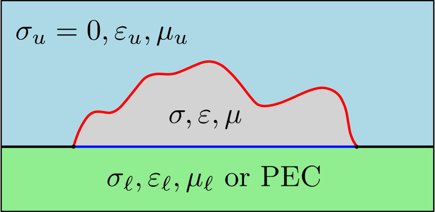
(a) Dielectric bump on a half-plane.

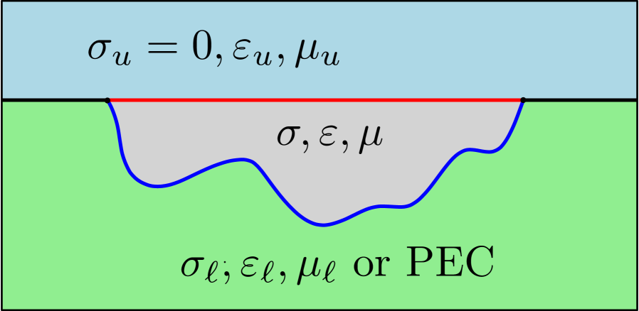
(b) Dielectric-filled cavity on a half-plane.

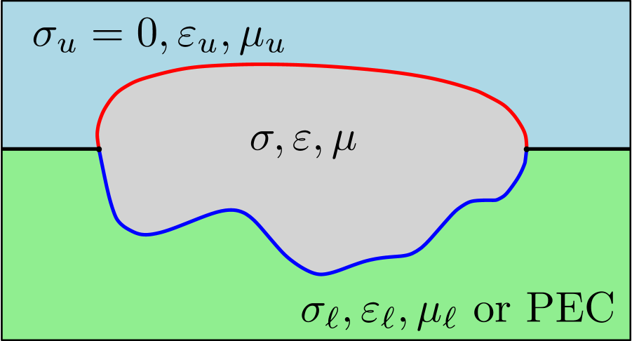
(c) Dielectric-overfilled cavity on a half-plane.

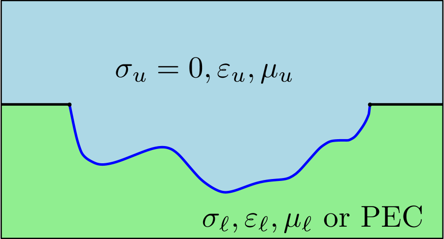
(d) Void cavity on a half-plane.

Figure 1: Schematics of the eight physical problems considered in this paper.

This paper presents high-order integral equation methods for the numerical solution of problems of scattering of a plane electromagnetic wave by cylindrical dielectric defects at the interface between two half-planes. Eight such classical problems are tackled in this contribution: scattering by a dielectric bump on 1) a perfectly electrically conducting (PEC) or 2) a dielectric half-plane (Fig. 1(a)); scattering by a dielectric-filled cavity on 3) a perfectly-conducting or 4) a dielectric half-plane (Fig. 1(b)); scattering by a dielectric-overfilled cavity on 5) a perfectly-conducting or 6) a dielectric half-plane (Fig. 1(c)); and scattering by a void cavity on 7) a perfectly-conducting or 8) a dielectric half-plane (Fig. 1(d)). From a mathematical perspective these eight different physical problems reduce to just three problem types for which this paper provides numerical solutions on the basis of highly accurate and efficient boundary integral equation methods.

In all cases the proposed methods utilize field representations based on single-layer potentials for appropriately chosen Green functions. As is known, such single-layer formulations lead to non-invertible integral equations at certain spurious resonances—that is, for wavenumbers that coincide with interior Dirichlet eigenvalues for a certain differential operator—either the Laplace operator or an elliptic differential operator with piecewise constant coefficients (see Sec. 4.2 for details). We nevertheless show that solutions for all wavenumbers can be obtained from such non-invertible formulations—including wavenumbers at which non-invertible integral equations result. Our method in these regards relies on the analyticity of the PDE solution as a function of the wavenumber together with a certain approach based on use of Chebyshev approximation.

(The use of field representations which give rise to non-invertible operators is advantageous in two main ways: on one hand this strategy allows one to bypass the need to utilize hypersingular operators, whose evaluation is computationally expensive and, otherwise, highly challenging near corner points; and, on the other hand, it leads to systems of integral equations containing fewer integral operators—with associated reduced computational cost.)

The problems considered in this paper draw considerable interest in a wide range of settings. For example, the problem of scattering by bumps and cavities on a (perfect or imperfect) conducting half-plane is important in the study of the radio-frequency absorption and electric and magnetic field enhancement that arises from surface roughness [28, 40]. The problem of scattering by open groove cavities on a conducting plane, in turn, impacts on a variety of technologies, with applicability to design of cavity-backed antennas, non-destructive evaluation of material surfaces, and more recently, modeling of extraordinary transmission of light and plasmonics resonance, amongst many others (e.g. [3] and references therein).

There is vast literature concerning the types of problems considered in this paper. For a circular bump a separation-of-variables analytical Fourier-Bessel expansion exists [27]. Related semi-analytical separation-of-variables solutions are available for other simple configurations, such as semi-circular cavities and rectangular bumps and cavities (e.g. [8, 9, 13, 19, 24, 23, 25, 31, 32, 39] and references therein), while solutions based on Fourier-type integral representations, mode matching techniques and staircase approximation of the geometry are available for more general domains (e.g. [5] and references therein). Even for simple configurations, such as a circular cavity or bump on a perfectly conduction plane, the semi-analytical separation-of-variables method requires solution of an infinite dimensional linear system of equations that must be truncated to an $n\times n$ system and solved numerically [14, 24, 25, 29, 31, 32]. As it happens, the resulting (full) matrix is extremely ill-conditioned for large values of $n$. In practice only limited accuracy results from use of such algorithms: use of small values of $n$ naturally produces limited accuracy, while for large values of $n$ matrix ill-conditioning arises as an accuracy limiting element.

Finite element and finite difference methods of low order of accuracy have been used extensively over the last decade [2, 3, 4, 12, 20, 33, 36, 37]. As is well known, finite element and finite difference methods lead to sparse linear systems. However, in order to satisfy the Sommerfeld radiation condition at infinity, a relatively large computational domain containing the scatterer must be utilized (unless a non-local boundary condition is used, with a consequent loss of sparsity). In view of the large required computational domains (or large coupled systems of equations for methods that use non-local domain truncation) and their low-order convergence (especially around corners where fields are singular and currents are infinite), these methods yield very slow convergence, and, therefore, for adequately accurate solutions, they require use of large numbers of unknowns and a high computational cost.

Boundary integral equation methods, on the other hand, lead to linear systems of reduced dimensionality, the associated solutions automatically satisfy the condition of radiation at infinity, and, unlike finite element methods, they do not suffer from dispersion errors. Integral equation methods have been used previously for the solution of the problem of scattering by an empty and dielectric-filled cavity on a perfectly conducting half-plane; see e.g. [15, 38, 35]. However, previous integral approaches for these problems are based on use of low-order numerical algorithms and, most importantly, they do not accurately account for singular field behavior at corners—and, thus, they may not be sufficiently accurate for evaluation of important physical mechanisms that arise from singular electrical currents and local fields at and around corners.

The present paper is organized as follows. Sec. 2 presents a brief description of the various problems at hand and Sec. 3 introduces a new set of integral equations for their treatment. Sec. 4 then describes the high-order solvers we have developed for the numerical solution of these integral equations, which include full resolution of singular fields at corners. The excellent convergence properties of the equations and algorithms introduced in this text are demonstrated in Sec. 5. In particular, the high accuracy of the new methods in presence of corner singularities can be used to evaluate the effects of corner singularities on currents and local fields on and around bumps and cavities, and, thus, on important physical observables such as absorption, extraordinary transmission, cavity resonance, etc.

2 Scattering problem

All the problems considered in this contribution can be described mathematically following the compact depiction presented in Fig. 2. Thus, a plane wave $\mathbb{H}^{\mathrm{inc}}(\boldsymbol{x})=\mathbb{H}^{0}\operatorname{e}^{i\mathbb{k}\cdot\boldsymbol{x}}$, $\mathbb{E}^{\mathrm{inc}}(\boldsymbol{x})=\mathbb{E}^{0}\operatorname{e}^{i\mathbb{k}\cdot\boldsymbol{x}}$ with wave vector $\mathbb{k}=k_{3}(\cos\alpha,\sin\alpha)$ impinges on a cavity formed by the subdomains $\Omega_{1}$ and $\Omega_{2}$ which lies on the boundary of an otherwise planar horizontal interface between the infinite subdomains $\Omega_{3}$ and $\Omega_{4}$. As is well-known, the $z$ components $u=E_{z}$ and $u=H_{z}$ of the total electric and magnetic field satisfy the Helmholtz equation

$$\Delta u+k^{2}_{j}u=0\quad\mbox{in}\quad\Omega_{j},$$ (1)

where, letting $\omega>0$, $\varepsilon_{j}>0$, $\mu_{j}>0$ and $\sigma_{j}\geq 0$ denote the angular frequency, the electric permittivity, the magnetic permeability and the electrical conductivity, the wavenumber $k_{j}$ ($\Im(k_{j})>0$) is defined by $k^{2}_{j}=\omega^{2}(\varepsilon_{j}+i\sigma_{j}/\omega)\mu_{j}$, $1\leq j\leq 4$ . Throughout this paper it is assumed that $\Omega_{3}$ is a lossless medium ($\sigma_{3}=0$).

In order to formulate transmission problems for the transverse components of the electromagnetic field, $u$ is expressed as

$$u=\left\{\begin{array}[]{lcc}u_{1}&\mathrm{in}&\Omega_{1},\\ u_{2}&\mathrm{in}&\Omega_{2},\\ u_{3}+f&\mathrm{in}&\Omega_{3},\\ u_{4}+f&\mathrm{in}&\Omega_{4},\\ \end{array}\right.$$ (2)

where $f$ is the solution (presented below in this section) of the problem of scattering by the lower half-plane in absence of the dielectric defect.

Additionally, $u$ satisfies the transmission conditions

$$\begin{array}[]{rclcl}u_{i}-u_{j}&=&g,\vskip 6.0pt plus 2.0pt minus 2.0pt\\ \displaystyle\frac{1}{\beta_{i}}\frac{\partial u_{i}}{\partial{\mathbf{n}}}-\frac{1}{\beta_{j}}\frac{\partial u_{j}}{\partial{\mathbf{n}}}&=&\displaystyle\frac{1}{\beta_{j}}\frac{\partial g}{\partial{\mathbf{n}}},\end{array}$$ (3)

at the interface $\Gamma_{ij}$ between $\Omega_{i}$ and $\Omega_{j}$, where $\beta_{j}=\mu_{j}$ in TM-polarization and $\beta_{j}=\varepsilon_{j}+i\sigma_{j}/\omega$ in TE-polarization. For each one of the problems considered in this paper Equations (3) with $g=f$ are satisfied on $\Gamma_{13}$. In the case in which $\Omega_{4}$ is filled by a dielectric material the transmission conditions (3) are also satisfied with boundary data $g=f$ on $\Gamma_{24}$, and they are satisfied with boundary data $g=0$ on $\Gamma_{34}$. On the other hand, when $\Omega_{4}$ is a perfectly conducting half-plane, $u_{4}=0$ and boundary conditions

$$u_{j}=0\quad\mbox{and}\quad\frac{\partial u_{j}}{\partial{\mathbf{n}}}=0,\quad j=2,3$$ (4)

are satisfied on $\Gamma_{j4}$ in TM- and TE-polarization, respectively. Additionally, the scattering fields $u_{j}$, $j=3,4$ fulfill the Sommerfeld radiation condition at infinity.

The solution $f$ of the problem of scattering by the lower half-plane in absence of the dielectric defect (which provides the necessary source term in (2)) can be computed explicitly for each one of the problems considered in this paper. For the problems in which $\Omega_{4}$ is a perfectly flat PEC half-plane the total field is given by $f(\boldsymbol{x})=E^{0}_{z}(\operatorname{e}^{i\mathbb{k}\cdot\boldsymbol{x}}-\operatorname{e}^{i\overline{\mathbb{k}}\cdot\boldsymbol{x}})$ in TM-polarization, and $f(\boldsymbol{x})=H^{0}_{z}(\operatorname{e}^{i\mathbb{k}\cdot\boldsymbol{x}}+\operatorname{e}^{i\overline{\mathbb{k}}\cdot\boldsymbol{x}})$ in TE-polarization, where $\mathbb{k}=k_{3}(\cos\alpha,\sin\alpha)$ and $\overline{\mathbb{k}}=k_{3}(\cos\alpha,-\sin\alpha)$. For the problems in which $\Omega_{4}$ is a flat dielectric half-plane, in turn, the total field is given by

$$f(\boldsymbol{x})=\left\{\begin{array}[]{ccc}E^{0}_{z}(\operatorname{e}^{i\mathbb{k}\cdot\boldsymbol{x}}+R^{\mbox{\tiny TM}}\operatorname{e}^{i\bar{\mathbb{k}}\cdot\boldsymbol{x}})&\mathrm{in}&\Omega_{3},\\ E^{0}_{z}T^{\mbox{\tiny TM}}\operatorname{e}^{i\widetilde{\mathbb{k}}\cdot\boldsymbol{x}}&\mathrm{in}&\Omega_{4},\end{array}\right.$$

and

$$f(\boldsymbol{x})=\left\{\begin{array}[]{ccc}H^{0}_{z}(\operatorname{e}^{i\mathbb{k}\cdot\boldsymbol{x}}+R^{\mbox{\tiny TE}}\operatorname{e}^{i\bar{\mathbb{k}}\cdot\boldsymbol{x}})&\mathrm{in}&\Omega_{3},\\ H^{0}_{z}T^{\mbox{\tiny TE}}\operatorname{e}^{i\widetilde{\mathbb{k}}\cdot\boldsymbol{x}}&\mathrm{in}&\Omega_{4},\end{array}\right.$$

in TM- and TE-polarization respectively, where

$$T^{\mathrm{TM,TE}}=\frac{2\beta_{4}k_{3}}{\beta_{4}k_{3}+\lambda\beta_{3}k_{4}},\quad R^{\mathrm{TM,TE}}=\frac{\beta_{4}k_{3}-\lambda\beta_{3}k_{4}}{\beta_{4}k_{3}+\lambda\beta_{3}k_{4}},\quad\lambda=\frac{\sqrt{1-k_{3}^{2}/k_{4}^{2}\cos^{2}(\alpha)}}{|\sin(\alpha)|}$$

and $\widetilde{\mathbb{k}}=k_{4}\left(k_{3}/k_{4}\cos(\alpha),-\sqrt{1-k_{3}^{2}/k_{4}^{2}\cos^{2}(\alpha)}\right)$ (using the square root function $\sqrt{z}$ determined by the relation $-\pi<\arg(z)\leq\pi$—so that, in particular, $\sqrt{-1}=i$).

3 Integral equation formulations

Three main problem types can be identified in connection with Fig. 2, namely Problem Type I, where transmission conditions (3) are imposed on $\Gamma_{13}$ and $\Gamma_{24}$ (which, in our context, characterize the problem of scattering by a dielectric bump on a dielectric half-plane as well as the problems of scattering by a filled, overfilled or empty cavity on a dielectric half-plane); Problem Type II, where transmission conditions (3) are imposed on $\Gamma_{13}$ and PEC boundary condition (4) is imposed on $\Gamma_{24}$, which applies to the problem of scattering by a (filled, overfilled or empty) cavity on a PEC half-plane; and Problem Type III, where transmission conditions (3) are only imposed on $\Gamma_{13}$, with application to the problem of scattering by a dielectric bump on a perfectly conducting half-plane. In the following three sections we derive systems of boundary integral equations for each one of these problem types.

Figure 2: Compact mathematical description of the problems considered in this paper.

3.1 Problem Type I

In Problem Type I the domains $\Omega_{j}$ ($1\leq j\leq 4$) contain dielectric media of finite or zero conductivity; we denote by $k_{j}$ the (real or complex) wavenumber in the domain $\Omega_{j}$. Note that

• For the problem of scattering by a dielectric-filled cavity on dielectric half-plane we have $k_{3}=k_{1},k_{1}\neq k_{2},k_{2}\neq k_{4}$;

• For the problem of scattering by an overfilled cavity on dielectric half-plane we have $k_{3}\neq k_{1},k_{1}=k_{2},k_{2}\neq k_{4}$; and

• For the problem of scattering by a void cavity on a dielectric half-plane we have $k_{3}=k_{1},k_{1}=k_{2},k_{2}\neq k_{4}$.

To tackle the Type I problem we express the total field $u$ by means the single-layer-potential representation

$$u=\left\{\begin{array}[]{lll}\mathcal{S}_{\mathrm{int}}[\psi_{\mathrm{int}}]&\mbox{in}&\Omega_{1}\cup\Omega_{2},\vskip 6.0pt plus 2.0pt minus 2.0pt\\ \mathcal{S}_{\mathrm{ext}}[\psi_{\mathrm{ext}}]+f&\mbox{in}&\Omega_{3}\cup\Omega_{4},\end{array}\right.$$ (5)

in terms of the unknown density functions $\psi_{\mathrm{int}}$ and $\psi_{\mathrm{ext}}$ where, letting $G_{k_{j}}^{k_{i}}$ denote the Green function of the Helmholtz equation for the two-layer medium with wavenumbers $k_{i}$ and $k_{j}$ in the upper and lower half-planes respectively (see Appendix C), we have set

$$\mathcal{S}_{\mathrm{int}}[\psi](\boldsymbol{x}) = \int_{\Gamma_{13}\cup\Gamma_{24}}G^{k_{1}}_{k_{2}}(\boldsymbol{x},\boldsymbol{y})\psi(\boldsymbol{y})\,\text{d}s_{\boldsymbol{y}},\vskip 6.0pt plus 2.0pt minus 2.0pt$$ (6a)

$$\mathcal{S}_{\mathrm{ext}}[\psi](\boldsymbol{x}) = \int_{\Gamma_{13}\cup\Gamma_{24}}G_{k_{4}}^{k_{3}}(\boldsymbol{x},\boldsymbol{y})\psi(\boldsymbol{y})\,\text{d}s_{\boldsymbol{y}}.$$ (6b)

The Green functions $G^{k_{i}}_{k_{j}}$ satisfy the transmission conditions (3) on $\Gamma_{ij}$ (with $(ij)$ equal to either $(12)$ or $(34)$) and, therefore, they depend on the polarization (through the parameters $\beta_{i}$ and $\beta_{j}$). Note, further, that for $k_{i}=k_{j}=k$ the Green function $G^{k_{i}}_{k_{j}}$ equals the free space Green function with wavenumber $k$.

It is easy to check that the representation (5) for the solution $u$ satisfies the Helmholtz equation with wavenumber $k_{j}$ in the domain $\Omega_{j}$ ($1\leq j\leq 4$) as well as the radiation conditions at infinity. Since the two-layer Green functions satisfy the relevant transmission conditions on $\Gamma_{12}$ and $\Gamma_{34}$, there remain only two boundary conditions to be satisfied, namely, the transmission conditions (3) on the boundary of the defect $\Omega_{1}\cup\Omega_{2}$. Using classical jump relations [10] for various layer potentials, these conditions lead to the system

$$\begin{array}[]{rrccl}\displaystyle S^{\Gamma_{13}}_{\mathrm{int}}[\psi_{\mathrm{int}}]-S^{\Gamma_{13}}_{\mathrm{ext}}[\psi_{\mathrm{ext}}]&=&f,\vskip 6.0pt plus 2.0pt minus 2.0pt\\ \displaystyle\frac{\beta_{3}}{\beta_{1}}\left\{\frac{\psi_{\mathrm{int}}}{2}-K^{\Gamma_{13}}_{\mathrm{int}}[\psi_{\mathrm{int}}]\right\}+\frac{\psi_{\mathrm{ext}}}{2}-K^{\Gamma_{13}}_{\mathrm{ext}}[\psi_{\mathrm{ext}}]&=&\displaystyle\frac{\partial f}{\partial{\mathbf{n}}},\vskip 6.0pt plus 2.0pt minus 2.0pt\\ \displaystyle S^{\Gamma_{24}}_{\mathrm{int}}[\psi_{\mathrm{int}}]-S^{\Gamma_{24}}_{\mathrm{ext}}[\psi_{\mathrm{ext}}]&=&f,\vskip 6.0pt plus 2.0pt minus 2.0pt\\ \displaystyle\frac{\beta_{4}}{\beta_{2}}\left\{\frac{\psi_{\mathrm{int}}}{2}-K^{\Gamma_{24}}_{\mathrm{int}}[\psi_{\mathrm{int}}]\right\}+\frac{\psi_{\mathrm{ext}}}{2}-K^{\Gamma_{24}}_{\mathrm{ext}}[\psi_{\mathrm{ext}}]&=&\displaystyle\frac{\partial f}{\partial{\mathbf{n}}}\end{array}$$ (7)

of boundary integral equations on the open curves $\Gamma_{13}$ and $\Gamma_{24}$ for the unknowns $\psi_{\mathrm{int}}$ and $\psi_{\mathrm{ext}}$. The boundary integral operators in (7) for $(ij)=(13)$ and $(ij)=(24)$ are given by

$$\begin{array}[]{l}S^{\Gamma_{ij}}_{\mathrm{int}}[\psi](\boldsymbol{x})=\displaystyle\int_{\Gamma_{13}\cup\Gamma_{24}}G^{k_{1}}_{k_{2}}(\boldsymbol{x},\boldsymbol{y})\psi(\boldsymbol{y})\,\text{d}s_{\boldsymbol{y}},\ \boldsymbol{x}\in\Gamma_{ij},\vskip 6.0pt plus 2.0pt minus 2.0pt\\ S^{\Gamma_{ij}}_{\mathrm{ext}}[\psi](\boldsymbol{x})=\displaystyle\int_{\Gamma_{13}\cup\Gamma_{24}}G_{k_{4}}^{k_{3}}(\boldsymbol{x},\boldsymbol{y})\psi(\boldsymbol{y})\,\text{d}s_{\boldsymbol{y}},\ \boldsymbol{x}\in\Gamma_{ij},\vskip 6.0pt plus 2.0pt minus 2.0pt\\ K^{\Gamma_{ij}}_{\mathrm{int}}[\psi](\boldsymbol{x})=\displaystyle\int_{\Gamma_{13}\cup\Gamma_{24}}\frac{\partial G^{k_{1}}_{k_{2}}}{\partial{\mathbf{n}}_{\boldsymbol{x}}}(\boldsymbol{x},\boldsymbol{y})\psi(\boldsymbol{y})\,\text{d}s_{\boldsymbol{y}},\ \boldsymbol{x}\in\Gamma_{ij},\vskip 6.0pt plus 2.0pt minus 2.0pt\\ K^{\Gamma_{ij}}_{\mathrm{ext}}[\psi](\boldsymbol{x})=\displaystyle\int_{\Gamma_{13}\cup\Gamma_{24}}\frac{\partial G_{k_{4}}^{k_{3}}}{\partial{\mathbf{n}}_{\boldsymbol{x}}}(\boldsymbol{x},\boldsymbol{y})\psi(\boldsymbol{y})\,\text{d}s_{\boldsymbol{y}},\ \boldsymbol{x}\in\Gamma_{ij}.\end{array}$$ (8)

3.2 Problem Type II

In Problem Type II the domain $\Omega_{4}$ contains a PEC medium, and the domains $\Omega_{j}$ ($1\leq j\leq 3$) contain dielectric media of finite or zero conductivity; we denote by $k_{j}$ the (real or complex) wavenumber in the domain $\Omega_{j}$ ($1\leq j\leq 3$). Clearly,

• For the problem of scattering by a dielectric-filled cavity on PEC half-plane we have $k_{3}=k_{1},k_{1}\neq k_{2}$;

• For the problem of scattering by an overfilled cavity on PEC half-plane we have $k_{3}\neq k_{1},k_{1}=k_{2}$; and

• For the problem of scattering by a void cavity on PEC half-plane we have $k_{3}=k_{1},k_{1}=k_{2}$.

For Type II problems we express the total field $u$ by means of the single-layer-potential representation

$$u=\left\{\begin{array}[]{lll}\mathcal{S}_{\mathrm{int}}[\psi_{\mathrm{int}}]&\mbox{in}&\Omega_{1}\cup\Omega_{2},\vskip 6.0pt plus 2.0pt minus 2.0pt\\ \mathcal{S}_{\mathrm{ext}}[\psi_{\mathrm{ext}}]+f&\mbox{in}&\Omega_{3},\vskip 6.0pt plus 2.0pt minus 2.0pt\\ 0&\mbox{in}&\Omega_{4},\end{array}\right.$$ (9)

where, defining $G^{k_{1}}_{k_{2}}$ as in Sec. 3.1 and letting $G^{k_{3}}_{\infty}$ denote the Green function that satisfies the PEC boundary condition (4) on $\Gamma_{34}$, the potentials above are defined by

$$\mathcal{S}_{\mathrm{int}}[\psi](\boldsymbol{x}) = \int_{\Gamma_{13}\cup\Gamma_{24}}G^{k_{1}}_{k_{2}}(\boldsymbol{x},\boldsymbol{y})\psi(\boldsymbol{y})\,\text{d}s_{\boldsymbol{y}},\vskip 6.0pt plus 2.0pt minus 2.0pt$$ (10a)

$$\mathcal{S}_{\mathrm{ext}}[\psi](\boldsymbol{x}) = \int_{\Gamma_{13}}G^{k_{3}}_{\infty}(\boldsymbol{x},\boldsymbol{y})\psi(\boldsymbol{y})\,\text{d}s_{\boldsymbol{y}}.$$ (10b)

As mentioned in Sec. 3.1 the Green function $G^{k_{i}}_{k_{j}}$ depends on the polarization; the same is of course true for $G^{k_{3}}_{\infty}$, which is given by $G^{k}_{\infty}(\boldsymbol{x},\boldsymbol{y})=G_{k}(\boldsymbol{x},\boldsymbol{y})-G_{k}(\bar{\boldsymbol{x}},\boldsymbol{y})$ in TM-polarization, and $G_{\infty}^{k}(\boldsymbol{x},\boldsymbol{y})=G_{k}(\boldsymbol{x},\boldsymbol{y})+G_{k}(\bar{\boldsymbol{x}},\boldsymbol{y})$ in TE-polarization, where $\bar{\boldsymbol{x}}=(x_{1},-x_{2})$ and where $G_{k}(\boldsymbol{x},\boldsymbol{y})=iH_{0}^{(1)}(k|\boldsymbol{x}-\boldsymbol{y}|)/4$ is the free-space Green function. By virtue of the integral representation (9) the field satisfies the Helmholtz equation in the domain $\Omega_{j}$ with wavenumber $k_{j}$ ($1\leq j\leq 3$), the radiation condition at infinity, transmission conditions on $\Gamma_{12}$ and the PEC boundary conditions on $\Gamma_{24}$. Imposing the remaining transmission conditions (3) on $\Gamma_{13}$ and PEC boundary condition (4) of $\Gamma_{24}$, we obtain the equations

$$\begin{array}[]{rcl}\displaystyle S^{\Gamma_{13}}_{\mathrm{int}}[\psi_{\mathrm{int}}]-S^{\Gamma_{13}}_{\mathrm{ext}}[\psi_{\mathrm{ext}}]&=&f,\vskip 6.0pt plus 2.0pt minus 2.0pt\\ \displaystyle\frac{\beta_{3}}{\beta_{1}}\left\{\frac{\psi_{\mathrm{int}}}{2}-K^{\Gamma_{13}}_{\mathrm{int}}[\psi_{\mathrm{int}}]\right\}+\frac{\psi_{\mathrm{ext}}}{2}-K^{\Gamma_{13}}_{\mathrm{ext}}[\psi_{\mathrm{ext}}]&=&\displaystyle\frac{\partial f}{\partial{\mathbf{n}}},\end{array}$$ (11a)

on $$\Gamma_{13} \beta_{j}$$ (valid for both TE and TM polarizations provided the corresponding constants  and Green functions are used) and

$$\frac{\psi_{\mathrm{int}}}{2}+K^{\Gamma_{24}}_{\mathrm{int}}[\psi_{\mathrm{int}}]=0\quad(\mbox{TE polarization})\vskip 6.0pt plus 2.0pt minus 2.0pt$$ (11b)

$$S^{\Gamma_{24}}_{\mathrm{int}}[\psi_{\mathrm{int}}]=0\quad(\mbox{TM polarization})$$ (11c)

on $\Gamma_{24}$. In accordance with the definition of the single-layer potentials (10), the boundary integral operators in (11) for $(ij)=(13)$ and $(ij)=(24)$ are given by

$$\begin{array}[]{l}S^{\Gamma_{ij}}_{\mathrm{int}}[\psi](\boldsymbol{x})=\displaystyle\int_{\Gamma_{13}\cup\Gamma_{24}}G^{k_{1}}_{k_{2}}(\boldsymbol{x},\boldsymbol{y})\psi(\boldsymbol{y})\,\text{d}s_{\boldsymbol{y}},\ \boldsymbol{x}\in\Gamma_{ij},\vskip 6.0pt plus 2.0pt minus 2.0pt\\ S^{\Gamma_{ij}}_{\mathrm{ext}}[\psi](\boldsymbol{x})=\displaystyle\int_{\Gamma_{13}}G^{k_{3}}_{\infty}(\boldsymbol{x},\boldsymbol{y})\psi(\boldsymbol{y})\,\text{d}s_{\boldsymbol{y}},\ \boldsymbol{x}\in\Gamma_{ij},\vskip 6.0pt plus 2.0pt minus 2.0pt\\ K^{\Gamma_{ij}}_{\mathrm{int}}[\psi](\boldsymbol{x})=\displaystyle\int_{\Gamma_{13}\cup\Gamma_{24}}\frac{\partial G^{k_{1}}_{k_{2}}}{\partial{\mathbf{n}}_{\boldsymbol{x}}}(\boldsymbol{x},\boldsymbol{y})\psi(\boldsymbol{y})\,\text{d}s_{\boldsymbol{y}},\ \boldsymbol{x}\in\Gamma_{ij},\vskip 6.0pt plus 2.0pt minus 2.0pt\\ K^{\Gamma_{ij}}_{\mathrm{ext}}[\psi](\boldsymbol{x})=\displaystyle\int_{\Gamma_{13}}\frac{\partial G_{\infty}^{k_{3}}}{\partial{\mathbf{n}}_{\boldsymbol{x}}}(\boldsymbol{x},\boldsymbol{y})\psi(\boldsymbol{y})\,\text{d}s_{\boldsymbol{y}},\ \boldsymbol{x}\in\Gamma_{ij}.\end{array}$$ (12)

3.3 Problem Type III

For Problem Type III the domains $\Omega_{j}$ ($j=1,3$) contain dielectric media of finite or zero conductivity (the corresponding, possibly complex, wavenumbers are denoted by $k_{1}$ and $k_{3}$), and the domains $\Omega_{j}$, $j=2,4,$ contain a PEC medium. Note that

• For the problem of scattering by a dielectric bump on PEC half-plane we have $k_{3}\neq k_{1}$.

As in the previous cases, for Type III problems the total field $u$ is expressed by means of the single-layer-potential representation

$$u=\left\{\begin{array}[]{lll}\mathcal{S}_{\mathrm{int}}[\psi_{\mathrm{int}}]&\mbox{in}&\Omega_{1},\vskip 6.0pt plus 2.0pt minus 2.0pt\\ \mathcal{S}_{\mathrm{ext}}[\psi_{\mathrm{ext}}]+f&\mbox{in}&\Omega_{3},\vskip 6.0pt plus 2.0pt minus 2.0pt\\ 0&\mbox{in}&\Omega_{2}\cup\Omega_{4},\end{array}\right.$$ (13)

where the potentials above are defined by

$$\mathcal{S}_{\mathrm{int}}[\psi](\boldsymbol{x}) = \int_{\Gamma_{13}}G^{k_{1}}_{\infty}(\boldsymbol{x},\boldsymbol{y})\psi(\boldsymbol{y})\,\text{d}s_{\boldsymbol{y}},\vskip 6.0pt plus 2.0pt minus 2.0pt$$ (14a)

$$\mathcal{S}_{\mathrm{ext}}[\psi](\boldsymbol{x}) = \int_{\Gamma_{13}}G^{k_{3}}_{\infty}(\boldsymbol{x},\boldsymbol{y})\psi(\boldsymbol{y})\,\text{d}s_{\boldsymbol{y}}.$$ (14b)

As mentioned in Sec. 3.2, the Green functions $G_{\infty}^{k_{1}}$ and $G_{\infty}^{k_{3}}$ depend on the polarization and satisfy the PEC boundary condition on $\Gamma_{12}$ and $\Gamma_{34}$ respectively. The total field, as given by the potentials (14), satisfies Helmholtz equations with wavenumber $k_{j}$ in the domain $\Omega_{j}$, $j=1,3$, PEC boundary condition on $\Gamma_{24}$ and $\Gamma_{12}$, as well as the radiation condition at infinity. Imposing the transmission conditions (3) on $\Gamma_{13}$ the following system of boundary integral equations is obtained for the unknown density functions $\psi_{\mathrm{int}}$ and $\psi_{\mathrm{ext}}$:

$$\begin{array}[]{rcl}\displaystyle S^{\Gamma_{13}}_{\mathrm{int}}[\psi_{\mathrm{int}}]-S^{\Gamma_{13}}_{\mathrm{ext}}[\psi_{\mathrm{ext}}]&=&f,\vskip 6.0pt plus 2.0pt minus 2.0pt\\ \displaystyle\frac{\beta_{3}}{\beta_{1}}\left\{\frac{\psi_{\mathrm{int}}}{2}-K^{\Gamma_{13}}_{\mathrm{int}}[\psi_{\mathrm{int}}]\right\}+\frac{\psi_{\mathrm{ext}}}{2}-K^{\Gamma_{13}}_{\mathrm{ext}}[\psi_{\mathrm{ext}}]&=&\displaystyle\frac{\partial f}{\partial{\mathbf{n}}},\end{array}$$ (15)

on $\Gamma_{13}$, where the boundary integral operators are defined by

$$\begin{array}[]{l}S^{\Gamma_{13}}_{\mathrm{int}}[\psi](\boldsymbol{x})=\displaystyle\int_{\Gamma_{13}}G^{k_{1}}_{\infty}(\boldsymbol{x},\boldsymbol{y})\psi(\boldsymbol{y})\,\text{d}s_{\boldsymbol{y}},\ \boldsymbol{x}\in\Gamma_{13},\vskip 6.0pt plus 2.0pt minus 2.0pt\\ S^{\Gamma_{13}}_{\mathrm{ext}}[\psi](\boldsymbol{x})=\displaystyle\int_{\Gamma_{13}}G^{k_{3}}_{\infty}(\boldsymbol{x},\boldsymbol{y})\psi(\boldsymbol{y})\,\text{d}s_{\boldsymbol{y}},\ \boldsymbol{x}\in\Gamma_{13},\vskip 6.0pt plus 2.0pt minus 2.0pt\\ K^{\Gamma_{13}}_{\mathrm{int}}[\psi](\boldsymbol{x})=\displaystyle\int_{\Gamma_{13}}\frac{\partial G^{k_{1}}_{\infty}}{\partial{\mathbf{n}}_{\boldsymbol{x}}}(\boldsymbol{x},\boldsymbol{y})\psi(\boldsymbol{y})\,\text{d}s_{\boldsymbol{y}},\ \boldsymbol{x}\in\Gamma_{13},\vskip 6.0pt plus 2.0pt minus 2.0pt\\ K^{\Gamma_{13}}_{\mathrm{ext}}[\psi](\boldsymbol{x})=\displaystyle\int_{\Gamma_{13}}\frac{\partial G_{\infty}^{k_{3}}}{\partial{\mathbf{n}}_{\boldsymbol{x}}}(\boldsymbol{x},\boldsymbol{y})\psi(\boldsymbol{y})\,\text{d}s_{\boldsymbol{y}},\ \boldsymbol{x}\in\Gamma_{13}.\end{array}$$ (16)

4 Numerical method

4.1 Discretization of integral equations

The integral equations (7), (11) and (15) involve either a) Integrals over $\Gamma_{13}\cup\Gamma_{24}$ with equality enforced on $\Gamma_{13}\cup\Gamma_{24}$, or given by b) Integrals over $\Gamma_{13}$ with equality enforced on $\Gamma_{13}$. All of these integral equations can be expressed in terms of parametrizations of the curves $\Gamma_{13}$ and $\Gamma_{24}$, or, more precisely, in terms of integrals of the form

$$\int_{0}^{2\pi}L(t,\tau)\phi(\tau)\,\text{d}\tau \int_{0}^{2\pi}M(t,\tau)\phi(\tau)\,\text{d}\tau,$$ and (17)

with kernels

$$\begin{array}[]{rcl}L(t,\tau)&=&\displaystyle G(\boldsymbol{x}(t),\boldsymbol{y}(\tau))|\boldsymbol{y}^{\prime}(\tau)|,\vskip 6.0pt plus 2.0pt minus 2.0pt\\ M(t,\tau)&=&\displaystyle\nabla_{\boldsymbol{x}}[G](\boldsymbol{x}(t),\boldsymbol{y}(\tau))\cdot{\mathbf{n}}(t)|\boldsymbol{y}^{\prime}(\tau)|\end{array}$$ (18)

where i) Each of the functions $\boldsymbol{x}(t)$ and $\boldsymbol{y}(\tau)$ denote either a parametrization for the curve $\Gamma_{13}$ or of the curve $\Gamma_{24}$ with parameters $t$ and $\tau$ in the interval $(0,2\pi)$; ii) ${\mathbf{n}}(t)=(x^{\prime}_{2}(t),-x^{\prime}_{1}(t))/|\boldsymbol{x}^{\prime}(t)|$ denotes the unit normal on $\Gamma_{13}$ or $\Gamma_{24}$, as appropriate, which points outward from the defect; iii) $\phi(\tau)=\psi(\boldsymbol{y}(\tau))$, where $\psi$ stands for the unknown density function under consideration; and iv) $G$ denotes the relevant Green function. Indeed, in case a) above, the integral over $\Gamma_{13}\cup\Gamma_{24}$ can be expressed as a sum of integrals on $\Gamma_{13}$ and $\Gamma_{24}$. In case b), in particular, we take $\boldsymbol{x}=\boldsymbol{y}$.

Our discretization of the integral equations (7), (11) and (15) is based on corresponding discretizations of the integrals (17). Following [10] we thus proceed by expressing the kernels (18) in the form

$$L(t,\tau) = L_{1}(t,\tau)\log r^{2}(t,\tau)+L_{2}(t,\tau),\vskip 6.0pt plus 2.0pt minus 2.0pt$$ (19a)

$$M(t,\tau) = M_{1}(t,\tau)\log r^{2}(t,\tau)+M_{2}(t,\tau),\$$ (19b)

where $L_{j}$ and $M_{j}$ ($j=1,2$) are smooth functions on $(0,2\pi)\times(0,2\pi)$ and where $\mathbf{r}(t,\tau)=\boldsymbol{x}(t)-\boldsymbol{y}(\tau)$ and $r(t,\tau)=|\mathbf{r}(t,\tau)|$. In cases for which $\boldsymbol{x}(t)$ and $\boldsymbol{y}(\tau)$ parametrize the same open curve we have

$$L_{1}(t,\tau) = -\frac{1}{4\pi}J_{0}(kr(t,\tau))|\boldsymbol{y}^{\prime}(\tau)|,\vskip 6.0pt plus 2.0pt minus 2.0pt$$

$$L_{2}(t,\tau) = L(t,\tau)-L_{1}(t,\tau)\log r^{2}(t,\tau),\vskip 6.0pt plus 2.0pt minus 2.0pt$$

$$M_{1}(t,\tau) = \frac{k}{4\pi}J_{1}(kr(t,\tau)){\mathbf{n}}(t)\cdot\frac{\mathbf{r}(t,\tau)}{r}|\boldsymbol{y}^{\prime}(\tau)|,\vskip 6.0pt plus 2.0pt minus 2.0pt$$

$$M_{2}(t,\tau) = M(t,\tau)-M_{1}(t,\tau)\log r^{2}(t,\tau).$$

The diagonal terms $L_{2}(t,t)$ and $M_{2}(t,t)$ can be computed exactly by taking the limit of $L_{2}(t,\tau)$ and $M_{2}(t,\tau)$ as $\tau\rightarrow t$ (see [10, p. 77] for details). On the other hand, when $\boldsymbol{x}(t)$ and $\boldsymbol{y}(\tau)$ parametrize different curves, $L$ and $M$ are smooth on $(0,2\pi)\times(0,2\pi)$ and, thus, $L_{1}=0$, $L=L_{2}$, $M_{1}=0$ and $M=M_{2}$. (Note that although in the latter case $L$ and $M$ are smooth functions, these functions are in fact nearly singular, for $t$ near the endpoints of the parameter interval $(0,2\pi)$ for the curve $\boldsymbol{x}$, and for $\tau$ around the corresponding endpoint of the parameter interval for the curve $\boldsymbol{y}$.)

Letting $K$ denote one of the integral kernels $L$ or $M$ in equation (19), in view of the discussion above $K$ may be expressed in the form $K(t,\tau)=K_{1}(t,\tau)\log r^{2}(t,\tau)+K_{2}(t,\tau)$ for smooth kernels $K_{1}$ and $K_{2}$. For a fixed $t$ then, there are two types of integrands for which high-order quadratures must be provided, namely integrands that are smooth in $(0,2\pi)$ but have singularities at the endpoints of the interval (that arise from corresponding singularities of the densities $\phi$ at the endpoints of the open curves; cf. [21, 34, 7]), and integrands that additionally have a logarithmic singularity at $\tau=t$. To handle both singular integration problems we follow [18, 10] and utilize a combination of a graded-meshes, the trapezoidal quadrature rule, and a quadrature rule that incorporates the logarithmic singularity into its quadrature weights—as described in what follows. Interestingly, the graded meshes and associated changes of variables gives rise to accurate integration even in the near-singular regions mentioned above in this section.

To introduce graded meshes we consider the polynomial change of variables $t=w(s)$ where

$$w(s) = 2\pi\frac{[v(s)]^{p}}{[v(s)]^{p}+[v(2\pi-s)]^{p}},\quad 0\leq s\leq 2\pi,$$ (20)

$$v(s) = \left(\frac{1}{p}-\frac{1}{2}\right)\left(\frac{\pi-s}{\pi}\right)^{3}+\frac{1}{p}\frac{s-\pi}{\pi}+\frac{1}{2},$$

and where $p\geq 2$. The function $w$ is smooth and increasing on $[0,2\pi]$, with $w^{(k)}(0)=w^{(k)}(2\pi)=0$ for $1\leq k\leq p-1$. Using this transformation we express $K$ as

$$K(t,\tau) = K(w(s),w(\sigma))$$

$$= K_{1}(w(s),w(\sigma))\log\left(4\sin^{2}\frac{s-\sigma}{2}\right)+\widetilde{K}_{2}(s,\sigma)$$

where

$$\widetilde{K}_{2}(s,\sigma) = K_{1}(w(s),w(\sigma))\log\left(\frac{r^{2}(w(s),w(\sigma))}{4\sin^{2}\frac{s-\sigma}{2}}\right)+K_{2}(w(s),w(\sigma)),$$

and where the diagonal term is given by $\widetilde{K}_{2}(s,\sigma)=2K_{1}(t,t)\log(w^{\prime}(s)|\boldsymbol{x}^{\prime}(t)|)+K_{2}(t,t)$. High-order accurate quadrature formulae for the integral operators (17) based on the $(2n-1)$–point discretization $\sigma_{j}=j\pi/n$ ($1\leq j\leq 2n-1$, corresponding to integration over the curve parametrized by $\boldsymbol{y}(\tau)$) at evaluation points $t=t_{i}=w(s_{i})$ with $s_{i}=i\pi/q$ ($1\leq i\leq 2q-1$, corresponding to evaluation of the operator at points on the curve parametrized by $\boldsymbol{x}(t)$) can easily be obtained [10] from the expressions

$$\int_{0}^{2\pi}f(\sigma)\,\text{d}\sigma\approx\frac{\pi}{n}\sum_{j=0}^{2n-1}f(\sigma_{j})$$ (21)

and

$$\int_{0}^{2\pi}f(\sigma)\log\left(4\sin^{2}\frac{s-\sigma}{2}\right)\,\text{d}\sigma\approx\sum_{j=0}^{2n-1}R_{j}^{(n)}(s)f(\sigma_{j}),$$

$0\leq s\leq 2\pi$, (which, for smooth functions $f$, yield high-order accuracy), where the weights $R_{j}(s)$ are given by

$$R_{j}(s)=-\frac{2\pi}{n}\sum_{m=1}^{n-1}\frac{1}{m}\cos m(s-\sigma_{j})-\frac{\pi}{n^{2}}\cos n(s-\sigma_{j}).$$

Clearly setting $s=\sigma_{i}$ in this equation gives $R_{j}(\sigma_{i})=R_{|i-j|}$ where

$$R_{k}=-\frac{2\pi}{n}\sum_{m=1}^{n-1}\frac{1}{m}\cos\frac{mk\pi}{n}-\frac{(-1)^{k}\pi}{n^{2}}.$$

Using these quadrature points and weights and corresponding parameter values $t=t_{i}=w(s_{i})$ for the observation point ($s_{i}=i\pi/q$) we obtain the desired discrete approximation for the integrals (17): for an approximation $\phi_{j}\approx\phi(\tau_{j})=\phi(w(\sigma_{j}))$ we have

$$\begin{array}[]{c}\displaystyle\int_{0}^{2\pi}K(t_{i},\tau)\phi(\tau)\,\text{d}\tau\approx\sum_{j=1}^{2n-1}\left\{K_{1}(t_{i},\tau_{j})W_{ij}+K_{2}(t_{i},\tau_{j})\frac{\pi}{n}\right\}\phi_{j}\,w^{\prime}(\sigma_{j})\end{array}$$ (22)

for $1\leq i\leq 2q-1$, where $\tau_{j}=w(\sigma_{j})$ and where the quadrature weights are given by

$$W_{ij}=R_{|i-j|}+\frac{\pi}{n}\log\left(\frac{r^{2}(t_{i},t_{j})}{4\sin^{2}(s_{i}-s_{j})/2}\right).$$

Note that for sufficiently large values of $p$ the product $\phi(w(\sigma))w^{\prime}(\sigma)$, (an approximation of which appears in (22)) vanishes continuously at the endpoints of the parameter interval $[0,2\pi]$—even in cases for which, as it happens for corners or points of junction between multiple dielectric materials, $\phi(w(\sigma))$ tends to infinity at the endpoints.

The systems of boundary integral equations (7), (11) and (15) are discretized by means of applications of the quadrature rule (22) to the relevant integral operators (8), (12) and (16), respectively. This procedure leads to linear systems of algebraic equations for the unknown values of the density functions $\psi_{\mathrm{int}}$ and $\psi_{\mathrm{ext}}$ at the quadrature points. The presence of the weight $w^{\prime}(\sigma_{j})$ in (22), which multiplies the unknowns $\phi_{j}\approx\phi(\tau_{j})$ and which is very small for $\sigma_{j}$ close to $0$ and $2\pi$, however, gives rise to highly ill conditioned linear systems. To avoid this difficulty we resort to the change of unknown $\eta_{j}=\phi_{j}w^{\prime}(\sigma_{j})$ in (22); for the equations which contain terms of the form $\psi_{\mathrm{int}}/2$ and $\psi_{\mathrm{ext}}/2$ it is additionally necessary to multiply both sides of the equation by $w^{\prime}(\sigma_{j})$ to avoid small denominators. In what follows, the resulting discrete linear systems for the problems under consideration are generically denoted by $\mathbb{A}\boldsymbol{\eta}=\mathbb{f}$ where, in each case $\boldsymbol{\eta}$ is a vector that combines the unknowns that result from the discretization procedure described above in this section for the various boundary portions $\Gamma_{ij}$ (cf. Fig. 2). Once $\boldsymbol{\eta}$ has been found, the numerical approximation of the scattered fields at a given point $\boldsymbol{x}$ in space, which in what follows will be denoted by $\tilde{u}=\tilde{u}(\boldsymbol{x})$, can be obtained by consideration of the relevant representation (6), (10) or (14). For evaluation points $\boldsymbol{x}$ sufficiently far from the integration curves these integrals can be accurately approximated using the change of variable $t=w(s)$ together with the trapezoidal rule (21); for observation points near the integration curves, in turn, a procedure based on interpolation along a direction transverse to the curve is used (see [1] for details).

4.2 Solution at resonant and near-resonant frequencies

As mentioned in the introduction, despite the fact that each one of the physical problems considered in this contribution admit unique solutions for all frequencies $\omega$ and all physically admissible values of the dielectric constant and magnetic permeability, for certain values of $\omega$ spurious resonances occur: for such values of $\omega$ the systems of integral equations derived in Sec. 3 are not invertible. In fact, spurious resonances for these systems arise whenever the wavenumber $k_{3}$, which will also be denoted by $\kappa$ in what follows, is such that $-k_{3}^{2}=-\kappa^{2}$ equals a certain Dirichlet eigenvalue. (More precisely, letting $\varepsilon(x)$ and $\mu(x)$ denote the prescribed (piece-wise constant) permittivity and permeability, spurious resonances occur whenever $\kappa$ satisfies $\Delta u=-\kappa^{2}\varepsilon(x)\mu(x)u$ in $\Omega_{1}\cup\Omega_{2}$ for some nonzero function $u$ satisfying $u=0$ on $\partial(\Omega_{1}\cup\Omega_{2})$. This can be established e.g. taking into account ideas underlying uniqueness arguments of the type found in [11, Chapter 3]. Note, in particular, that the values of $\kappa$ for which spurious resonances occur are necessarily real numbers (and, thus, physically realizable), since the eigenvalues $-\kappa^{2}$ are necessarily negative).

It is important to note that, in addition to the spurious resonances mentioned above, the transmission problems considered in Sec. 2 themselves (and, therefore the corresponding systems of integral equations mentioned above) also suffer from non-uniqueness for certain non-physical values of $\kappa$ ($\Im(\kappa)<0$) which are known as “scattering poles” [30]; cf. Fig. 4 and a related discussion below in this section.

The non-invertibility of the aforementioned continuous systems of integral equations at a spurious-resonance or scattering-pole wavenumber $\kappa=\kappa^{*}$ manifests itself at the discrete level in non-invertibility or ill-conditioning of the system matrix $\mathbb{A}:=\mathbb{A}(\kappa)$ for values of $\kappa$ close to $\kappa^{*}$. Therefore, for $\kappa$ near $\kappa^{*}$ the numerical solution of the transmission problems under consideration (which, in what follows will be denoted by $\tilde{u}:=\tilde{u}_{\kappa}(\boldsymbol{x})$ to make explicit the solution dependence on the parameter $\kappa$) cannot be obtained via direct solution the linear system $\mathbb{A}\boldsymbol{\eta}=\mathbb{f}$. As is known, however [30], the solutions $u=u_{\kappa}$ of the continuous transmission problems are analytic functions of $\kappa$ for all real values of $\kappa$—including, in particular, for $\kappa$ equal to any one of the spurious resonances mentioned above and for real values of $\kappa$ near a scattering pole—and therefore, the approximate values $\tilde{u}_{\kappa}(\boldsymbol{x})$ for $\kappa$ sufficiently far from $\kappa^{*}$ can be used, via analytic continuation, to obtain corresponding approximations around $\kappa=\kappa^{*}$ and even at a spurious resonance $\kappa=\kappa^{*}$.

In order to implement this strategy for a given value of $\kappa$ it is necessary for our algorithm to possess a capability to perform two main tasks, namely, Task I: Determination of whether $\kappa$ is “sufficiently far” from any one of the spurious resonances and scattering poles $\kappa^{*}$; and Task II: Evaluation of analytic continuations to a given real wavenumber $\kappa_{0}$ which is either close or equal to a spurious resonance $\kappa^{*}$, or which lies close to a scattering pole $\kappa^{*}$. Once these capabilities are available the algorithm can be completed readily: if completion of Task I leads to the conclusion that $\kappa$ is far from all spurious resonances then the solution process proceeds directly via solution of the associated system of integral equations. Otherwise, the solution process is completed by carrying out Task II. Descriptions of the proposed methodologies to perform Tasks I and II are presented in the following two sections.

4.2.1 Task I: matrix-singularity detection

Consider a given wavenumber $\kappa^{\prime}$ for which a solution to one of the problems under consideration needs to be obtained. As discussed in what follows, in order to determine the level of proximity of $\kappa^{\prime}$ to a spurious resonance or scattering pole $\kappa^{*}$, the matrix-singularity detection algorithm utilizes the minimum singular value $\sigma_{\min}(\kappa^{\prime})$ of $\mathbb{A}(\kappa^{\prime})$. (Note that in view of the discussion concerning Task I above in the present Sec. 4.2 it is not necessary to differentiate wavenumbers $\kappa^{\prime}$ that lie near to either a spurious resonance or to a scattering pole: both cases can be treated equally well by means of one and the same Task II (analytic continuation) algorithm (Sec. 4.2.2).

To introduce the matrix-singularity detection algorithm consider Fig. 3: clearly, with exception of a sequence of wavenumbers (spurious resonances and/or real wavenumbers close to non-real scattering pole) around which the minimum singular value is small, the function $\sigma_{\min}(\kappa)$ maintains an essentially constant level. This property forms the basis of the matrix-singularity detection algorithm. Indeed, noting that there are no singularities for $\kappa$ smaller than certain threshold (as it follows from the spectral theory for the Laplace operator), we choose a wavenumber $\kappa_{0}>0$ close to zero and we compare $\sigma_{\min}(\kappa_{0})$ with $\sigma_{\min}(\kappa^{\prime})$. If $\sigma_{\min}(\kappa^{\prime})\ll\sigma_{\min}(\kappa_{0})$, say $\sigma_{\min}(\kappa^{\prime})<\xi\cdot\sigma_{\min}(\kappa_{0})$ for an adequately chosen value of $\xi$, $\kappa^{\prime}$ is determined to be close to a some singularity $\kappa^{*}$, and therefore the Task-II analytic-continuation algorithm is utilized to evaluate $\tilde{u}_{\kappa^{\prime}}(\boldsymbol{x})$. The parameter values $\kappa_{0}=0.1$ and $\xi=10^{-4}$ were used in all the numerical examples presented in this paper.

(A remark is in order concerning the manifestations of resonances and scattering poles on the plots of the function $\sigma_{\min}(\kappa)$ as a function of the real variable $\kappa$. By definition the function $\sigma_{\min}(\kappa)$ vanishes exactly at all spurious resonances. The four sharp peaks shown in Fig. 3, for example, occur at the spurious resonances listed in the inset of Fig. 4. The first peak from the left in Fig. 3, in contrast, is not sharp—as can be seen in the inset close-up included in the figure. The small value $\sigma_{\min}(\kappa)\sim 10^{-7}$ around $\kappa=0.5708$ is explained by the presence of a scattering pole $\kappa^{*}$: $\sigma_{\min}(\kappa^{*})=0$ at the complex wavenumber $\kappa^{*}=0.57807113743881-0.000074213015953i$. Thus scattering poles can in practice be quite close to the real $\kappa$ axis, and thus give rise to rather sharp peaks which are not associated with actual spurious resonances. As mentioned above, however, the analytic continuation algorithm presented in what follows need not differentiate between these two types of singularities: analytic continuation is utilized whenever a sufficiently small value of $\sigma_{\min}$ is detected.)

4.2.2 Task II: analytic continuation

Analytic continuation of the numerical solution $\tilde{u}_{\kappa}(\boldsymbol{x})$ to a given wavenumber $\kappa^{\prime}$ detected as a matrix singularity (Sec. 4.2.1) is carried out via interpolation. Note, however, that, since $\mathbf{A}(\kappa)$ is generally extremely ill-conditioned for values of $\kappa$ in a narrow interval around such wavenumbers $\kappa^{\prime}$, fine interpolation meshes cannot be utilized to achieve arbitrary accuracy in the approximation. To overcome this difficulty we utilize an interpolation method based on use of Chebyshev expansions, for which the meshsize is not allowed to be smaller than a certain tolerance, and within which convergence is achieved, in view of the analyticity of the scattered field with respect to the wavenumber $\kappa$, by increasing the order of the Chebyshev expansion. To do this for a given wavenumber $\kappa^{\prime}$ identified by the matrix-singularity detection algorithm (Sec. 4.2.1), the analytic continuation algorithm proceeds by introducing a Chebyshev grid of points $\{\kappa_{j}\}_{j=1}^{2m}$ (cf. [16]) sorted in ascending order such that the two middle points in the grid, $\kappa_{m}$ and $\kappa_{m+1}$, lie at an appropriately selected distance $\delta>0$ from the wavenumber $\kappa^{\prime}$: $\kappa_{m}=\kappa^{\prime}-\delta$ and $\kappa_{m+1}=\kappa^{\prime}+\delta$.

The accuracy of the numerical evaluation of the field $\tilde{u}_{\kappa_{j}}$ at each one of the interpolation points $\kappa_{j}$ is ensured by running the matrix-singularity detection algorithm at each $\kappa_{j}$ and adequately changing the value of $\delta$ if a matrix-singularity is detected at one or more of the mesh points $\kappa_{j}$. Letting $\tilde{u}^{(m)}_{\kappa}$ denote the Chebyshev expansion of order $2m-1$ resulting for a Chebyshev mesh selected as indicated above, the sequence $\tilde{u}^{(m)}_{\kappa^{\prime}}$ convergences exponentially fast to $\tilde{u}_{\kappa^{\prime}}$ as $m$ grows—as it befits Chebyshev expansions of analytic functions. If the matrix-singularity condition $\sigma_{\min}(\kappa_{j_{\ell}})<\xi\cdot\sigma_{\min}(\kappa_{0})$ occurs at one of more of the interpolation points $\kappa_{j}$, say $\kappa_{j_{\ell}}$, $1\leq\ell\leq L^{\prime}$, the algorithm proceeds by selecting the smallest value of the parameter $\delta^{\prime}>\delta$ and a new set of Chebyshev points $\{\kappa^{\prime}_{j}\}_{j=1}^{2m^{\prime}}$ ($m^{\prime}\geq m$) satisfying $\kappa^{\prime}_{m^{\prime}}=\kappa^{\prime}-\delta^{\prime}$, $\kappa^{\prime}_{m^{\prime}+1}=\kappa^{\prime}+\delta^{\prime}$, such that none of the new interpolation points lie on the region $\bigcup_{\ell=1}^{L^{\prime}}(\kappa_{j_{\ell}}-\delta,\kappa_{j_{\ell}}+\delta)$. If the condition $\sigma_{\min}(\kappa^{\prime}_{j})<\xi\cdot\sigma_{\min}(\kappa_{0})$ occurs for some of the new interpolation points, say $\kappa^{\prime}_{j_{\ell}}$, $1\leq\ell\leq L^{\prime\prime}$, the algorithm proceeds as described above, but for a new value $\delta^{\prime\prime}>\delta^{\prime}$, and so on. Note that in practice the interpolation procedure described above is rarely needed, and when it is needed, a suitable interpolation grid is usually found after a single iteration: in practice the choice $\delta=0.01$ has given excellent results in all the examples presented in this paper.

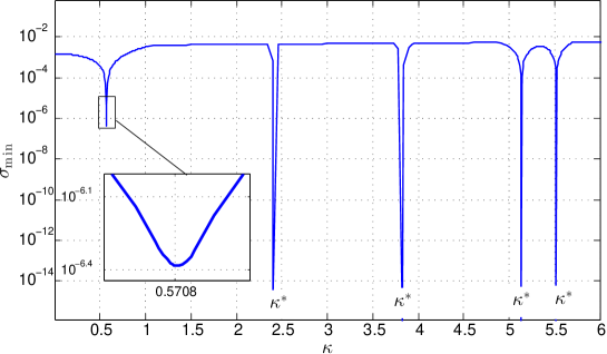
Figure 3: Minimum singular value of $\mathbb{A}$ as a function of $\kappa=k_{3}$ for the problem of scattering by a semi-circular bump on a PEC half-plane in TE-polarization.

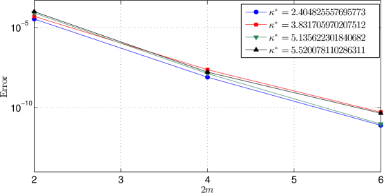
Figure 4: Error in the approximation of $\tilde{u}_{\kappa^{*}}$ by Chebyshev interpolation/analytic-continuation for various spurious resonant frequencies $\kappa^{*}$ as a function of the order $2m$ of the Chebyshev expansion.

In order to demonstrate the fast convergence of $\tilde{u}^{(m)}_{\kappa^{\prime}}$ to $\tilde{u}_{\kappa^{\prime}}$ as $m$ increases we consider the problem of scattering by a dielectric unit-radius semi-circular bump on a PEC half-plane. For this problem the wavenumbers $\kappa^{*}$ for which the system of integral equations (15) is non-invertible can be computed explicitly: spurious resonances are given by real solutions of the equation $J_{n}(\kappa)=0$, $n\geq 0$, where $J_{n}$ denotes the Bessel function of first kind and order $n$, and scattering poles are complex valued solutions of $\kappa H_{n}^{(1)}(\kappa)J_{n}^{\prime}(k_{1})=k_{1}J_{n}(k_{1}){H_{n}^{(1)}}^{\prime}(\kappa)$, where $H_{n}^{(1)}$ denotes the Hankel function of first kind and order $n$ (see Appendix. AB). The function $\sigma_{\min}(\kappa)$ is displayed in Fig. 3. The $\kappa^{*}$ values identified in that figure coincide (up to machine precision) with the first four positive solutions of the equation $J_{n}(\kappa)=0$. On the other hand, this problem admits an analytical solution $u_{\kappa}$ in terms of a Fourier-Bessel expansion (see Appendix A). The availability of the exact solution allows us to quantify the magnitude of interpolation error by evaluating the maximum of the error function $E(\boldsymbol{x})=|\tilde{u}^{(m)}_{\kappa^{*}}(\boldsymbol{x})-u_{\kappa^{*}}(\boldsymbol{x})|$ at a polar grid $\Pi$ (consisting of points inside, outside and at the boundary of the semi-circular bump). Fig. 4 shows the error $\max_{\boldsymbol{x}\in\Pi}E(\boldsymbol{x})$ versus the number of points used in the Chebyshev interpolation of $\tilde{u}_{\kappa^{*}}$, which is computed for the four spurious resonances $k^{*}$ shown in Fig. 3, and where a sufficiently fine spatial discretization is used. In all the calculations $k_{1}=6$, the curve $\Gamma_{13}$ is discretized using $128$ points, and $\delta=0.01$ is utilized to construct the Chebyshev grids.

5 Numerical results

This section demonstrates the high accuracies and high-order convergence that result as the proposed boundary integral methods are applied to each one of the mathematical problems formulated in Sec. 3. For definiteness all dielectric media are assumed non-magnetic so that $\beta_{i}/\beta_{j}=1$ for TM-polarization and $\beta_{i}/\beta_{j}=k_{i}^{2}/k_{j}^{2}$ for TE-polarization. In all the numerical examples shown in this section the incident plane-wave is parallel to the vector $d=(\cos(\pi/3),-\sin(\pi/3))$ and the graded-mesh parameter (20) is $p=8$.

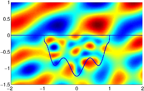
(a) TM-polarization.

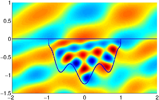
(b) TE-polarization.

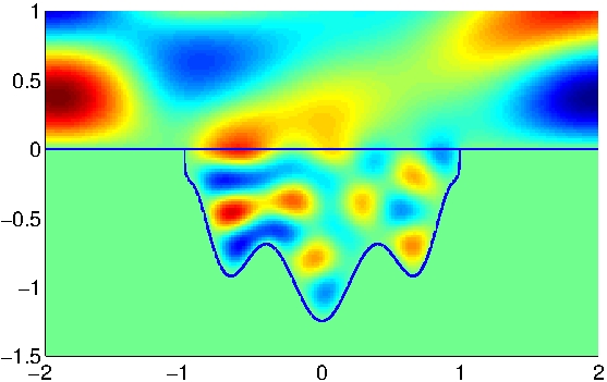
(c) TM-polarization.

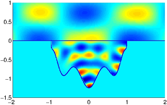
(d) TE-polarization.

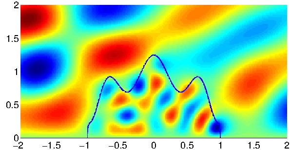
(e) TM-polarization.

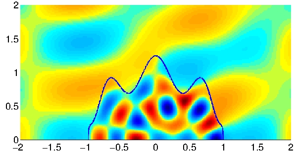
(f) TE-polarization.

Figure 5: Diffraction pattern resulting from the scattering of a plane-wave by; a dielectric-filled cavity on a dielectric half-plane ((a) and (b)); a dielectric-filled cavity on a PEC half-plane ((c) and (d)); a dielectric bump on a PEC half-plane ((e) and (f)).

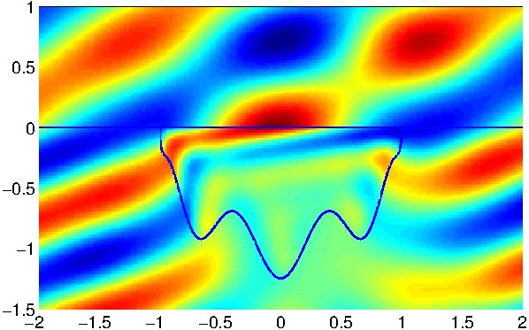
(a) TM-polarization.

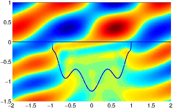
(b) TE-polarization.

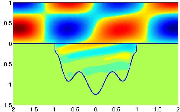
(c) TM-polarization.

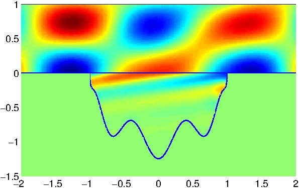
(d) TE-polarization.

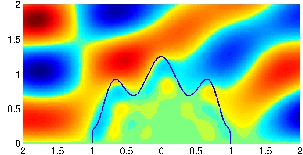
(e) TM-polarization.

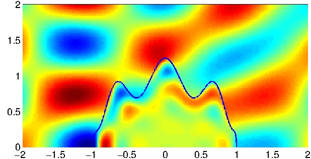
(f) TE-polarization.

Figure 6: Diffraction pattern resulting from the scattering of a plane-wave by; a dielectric-filled cavity on a dielectric half-plane ((a) and (b)); a dielectric-filled cavity on a PEC half-plane ((c) and (d)); a dielectric bump on a PEC half-plane ((e) and (f)).

We thus consider the problem of scattering by a dielectric filled cavity on a dielectric half-plane (problem type I); the problem of scattering by a dielectric filled cavity on a PEC half-plane (problem type II); and the problem of scattering by a dielectric bump on a PEC half-plane (problem type III). With reference to Fig. 2, in the first two examples the cavity is determined by the curve $\Gamma_{24}=\{(x,y)\in\mathbb{R}^{2}:x=-\cos(\frac{t}{2}),y=\frac{\cos(4t)}{40}t(t-2\pi)-\sin(\frac{t}{2}),t\in(0,2\pi)\}$, and the curve $\Gamma_{13}$ (which, in view of the formulation in Sec. 3, may be selected rather arbitrarily as long as it lies in the upper half plane and has the same endpoints as $\Gamma_{24}$) is given by the semicircle of radius one in the upper half plane that joins the points $(1,0)$ and $(-1,0)$. For the problem of scattering by a dielectric bump (type III problem), in turn, the boundary of the bump is given by $\Gamma_{13}=\{(x,y)\in\mathbb{R}^{2}:x=\cos(\frac{t}{2}),y=\frac{\cos(4t)}{40}t(2\pi-t)+\sin(\frac{t}{2}),t\in(0,2\pi)\}.$

To estimate the error in the aforementioned numerical test problems, the systems of boundary integral equations (7), (11) and (15) were discretized utilizing five different meshes $\Pi_{j}$, $1\leq j\leq 5$ consisting of $P=2^{j+5}-1$ points distributed along each one of the relevant boundaries: $P$ points on $\Gamma_{24}$ and $P$ points on $\Gamma_{13}$ in the case of type I and II problems, and $P$ points on $\Gamma_{13}$ in the case of type III problem. The sequence of meshes is chosen to be nested ($\Pi_{j}\subset\Pi_{i}$ for $j<i$) in order to facilitate the convergence analysis; in what follows the numerical solution that results from the discretization $\Pi_{j}$ is denoted by $\tilde{u}_{j}$. The error in the numerical solution $\tilde{u}_{j}$ is estimated by means of the expression

$$E_{j}=\frac{\max_{\boldsymbol{x}\in\Pi_{1}}|\tilde{u}_{j}(\boldsymbol{x})-\tilde{u}_{5}(\boldsymbol{x})|}{\max_{\boldsymbol{x}\in\Pi_{1}}|\tilde{u}_{5}(\boldsymbol{x})|},\quad 1\leq j\leq 4.$$

		Type I		Type II		Type III
		$k_{2}$		$k_{2}$		$k_{1}$
	$P$	$15$	$15+5i$	$15$	$15+5i$	$15$	$15+5i$
	63	$3\!\cdot\!10^{-01}$	$6\!\cdot\!10^{-03}$	$7\!\cdot\!10^{-01}$	$1\!\cdot\!10^{-04}$	$2\!\cdot\!10^{-01}$	$7\!\cdot\!10^{-02}$
TM	127	$7\!\cdot\!10^{-04}$	$4\!\cdot\!10^{-06}$	$2\!\cdot\!10^{-03}$	$1\!\cdot\!10^{-07}$	$2\!\cdot\!10^{-03}$	$1\!\cdot\!10^{-03}$
	255	$1\!\cdot\!10^{-10}$	$7\!\cdot\!10^{-12}$	$3\!\cdot\!10^{-11}$	$6\!\cdot\!10^{-12}$	$5\!\cdot\!10^{-08}$	$8\!\cdot\!10^{-08}$
	511	$6\!\cdot\!10^{-12}$	$5\!\cdot\!10^{-12}$	$1\!\cdot\!10^{-12}$	$3\!\cdot\!10^{-13}$	$1\!\cdot\!10^{-13}$	$8\!\cdot\!10^{-13}$
	63	$9\!\cdot\!10^{-02}$	$3\!\cdot\!10^{-03}$	$2\!\cdot\!10^{-01}$	$6\!\cdot\!10^{-04}$	$4\!\cdot\!10^{-01}$	$4\!\cdot\!10^{-02}$
TE	127	$3\!\cdot\!10^{-04}$	$7\!\cdot\!10^{-06}$	$1\!\cdot\!10^{-04}$	$2\!\cdot\!10^{-07}$	$1\!\cdot\!10^{-03}$	$3\!\cdot\!10^{-04}$
	255	$3\!\cdot\!10^{-12}$	$2\!\cdot\!10^{-12}$	$3\!\cdot\!10^{-12}$	$7\!\cdot\!10^{-12}$	$2\!\cdot\!10^{-08}$	$2\!\cdot\!10^{-08}$
	511	$1\!\cdot\!10^{-12}$	$2\!\cdot\!10^{-12}$	$4\!\cdot\!10^{-14}$	$1\!\cdot\!10^{-14}$	$1\!\cdot\!10^{-13}$	$2\!\cdot\!10^{-13}$

Table 1: Convergence test for the numerical solution of Problem Type I ($k_{1}=5$, $k_{2}=15$ or $15+5i$, $k_{3}=5$, and $k_{4}=7$), II ($k_{1}=5$, $k_{2}=15$ or $15+5i$, and $k_{3}=5$) and III ($k_{1}=15$ or $15+5i$, and $k_{3}=5$).

Table 1 presents the numerical error estimates $E_{j}$, $1\leq j\leq 5$ for the three different problem types (including real and complex wavenumbers); clearly high accuracies and fast convergence is achieved in all cases. To further illustrate the results provided by the proposed method, the real part of the total field is presented in Figs. 5 and 6 for the cases considered in Table 1, including examples for TM- and TE-polarization. Thus, Figs. 5(a)-5(b) ($k_{2}=15$) and Figs. 6(a)-6(b) ($k_{2}=15+5i$) present the diffraction pattern for the problem of scattering by the dielectric-filled cavity on the dielectric half-plane (problem Type I); Figs. 5(c)-5(d) ($k_{2}=15$) and Figs. 6(c)-6(d) ($k_{2}=15+5i$) present the diffraction pattern for the problem of scattering by the dielectric-filled cavity on the PEC half-plane (problem Type II); and Figs. 5(e)-5(f) ($k_{1}=15$) and Figs. 6(e)-6(f) ($k_{1}=15+5i$) present the diffraction pattern for the problem of scattering by the dielectric bump on the PEC half-plane.

Fig. 7, finally, presents diffraction patterns (real part) for the problem of scattering by a dielectric filled cavity on a dielectric half-plane (Problem Type I) for the wavenumbers $k_{1}=k_{3}=15$, $k_{2}=10$, $k_{4}=5$ and the angle of incidence $\alpha=-\pi/3$ in TM- and TE-polarization, as well as the corresponding transmission patterns for the dielectric half-plane in absence of the cavity. For these specially selected numerical values of the physical constants the phenomenon of total internal reflection [17] takes place: in absence of the cavity the field transmitted below the interface decays exponentially fast with the distance to the interface. Interestingly (although not surprisingly), placement of a defect in this configuration gives rise to transmission of electromagnetic radiation to the lower half plane.

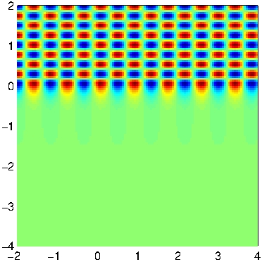
(a) TM-polarization.

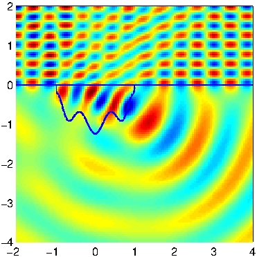
(b) TM-polarization.

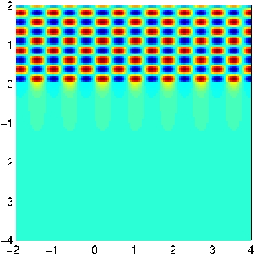
(c) TE-polarization.

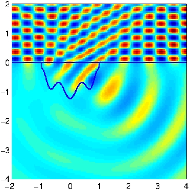
(d) TE-polarization.

Figure 7: Scattering and transmission of a plane-wave by a dielectric half plane in absence (resp. presence) of a dielectric-filled cavity (Problem Type I with wavenumbers $k_{1}=k_{3}=15$, $k_{2}=10$ and $k_{4}=5$. The parameters are selected in such a way to give rise to total internal reflection in absence of the cavity.

Acknowledgments. The authors gratefully acknowledge support from the Air Force Office of Scientific Research and the National Science Foundation.

Appendix A Semi-circular dielectric bump on PEC half-plane

For reference and testing we consider the problem of scattering of a plane-wave by a unit-radius semi-circular dielectric bump $\Omega_{1}=\{(r\cos\theta,r\sin\theta)\in\mathbb{R}^{2},0\leq r<1,0\leq\theta\leq\pi\}$ on a PEC half-plane $\Omega_{4}$ (Problem Type III), for which an exact solution in terms of a Fourier-Bessel expansion exists. In detail, the solution of (1) can expressed as

$$u_{1}(r,\theta) = \sum_{n=0}^{\infty}a_{n}J_{n}(k_{1}r)\Phi_{n}(\theta)\quad\mbox{in}\quad\Omega_{1},$$ (23a)

$$u_{3}(r,\theta) = \sum_{n=0}^{\infty}b_{n}H_{n}^{(1)}(k_{3}r)\Phi_{n}(\theta)\quad\mbox{in}\quad\Omega_{3},$$ (23b)

where $J_{n}$ and $H^{(1)}_{n}$ are the Bessel and Hankel functions of the first kind and order $n$, where $\Phi_{n}(\theta)=\cos(n\theta)$ in TE-polarization and $\Phi_{n}(\theta)=\sin(n\theta)$ in TM-polarization. The Fourier coefficients in (23) are given by

$$a_{n} = \frac{c_{n}k_{3}+(d_{n}-nc_{n})A_{n}}{\left[\frac{\beta_{3}}{\beta_{1}}k_{1}J^{\prime}_{n}(k_{1})-nJ_{n}(k_{1})\right]A_{n}+k_{3}J_{n}(k_{1})},$$

$$b_{n} = -\frac{c_{n}k_{1}+(\frac{\beta_{1}}{\beta_{3}}d_{n}-nc_{n})B_{n}}{\left[\frac{\beta_{1}}{\beta_{3}}k_{3}{H^{(1)}_{n}}^{\prime}(k_{3})-nH^{(1)}_{n}(k_{3})\right]B_{n}+k_{1}H^{(1)}_{n}(k_{3})},$$

where

$$A_{n}=\frac{H^{(1)}_{n}(k_{3})}{H^{(1)}_{n+1}(k_{3})},\quad B_{n}=\frac{J_{n}(k_{1})}{J_{n+1}(k_{1})},$$

$$c_{n} = \frac{2}{(1+\delta_{n0})\pi}\int_{0}^{\pi}f(1,\theta)\Phi_{n}(\theta)\,\text{d}\theta,$$

$$d_{n} = \frac{2}{(1+\delta_{n0})\pi}\int_{0}^{\pi}\frac{\partial f}{\partial r}(1,\theta)\Phi_{n}(\theta)\,\text{d}\theta.$$

Appendix B Scattering poles

As discussed in Sec. 4.2, scattering poles are complex wavenumbers $k$ for which there exists a non-trivial solution of a transmission problem without sources. In the context of the problem of a dielectric bump on a PEC half plane, for example, scattering poles correspond to existence of non-zero solutions of Problem Type III with $f=0$. In the particular case considered in Appendix A (semi-circular bump), the problem of evaluation of scattering poles can be further reduced to the problem of finding zeroes of certain nonlinear equations. Indeed, in order for $k_{3}$ to be a scattering pole the conditions

$$u_{1}=u_{3}\quad\mbox{and}\quad\frac{1}{\beta_{1}}\frac{\partial u_{1}}{\partial r}=\frac{1}{\beta_{3}}\frac{\partial u_{3}}{\partial r}$$

must be satisfied on the boundary $r=1$ of the bump. From eq. (23) it follows that $k_{3}$ is a scattering pole if and only if there exist non-trivial constants $a_{n}$ and $b_{n}$ such that

$$a_{n}J_{n}(k_{1})-b_{n}H_{n}^{(1)}(k_{3}) = 0,$$

$$a_{n}\frac{k_{1}J^{\prime}_{n}(k_{1})}{\beta_{1}}-b_{n}\frac{k_{3}{H^{(1)}_{n}}^{\prime}(k_{3})}{\beta_{3}} = 0$$

for some non-negative integer $n$. Clearly such constants exist if and only if the determinant of the matrix associated to the linear system above vanishes at $k_{3}$. Therefore, scattering poles are given by complex valued solutions $k_{3}$ of the equation

$$\frac{k_{1}}{\beta_{1}}H_{n}^{(1)}(k_{3})J_{n}^{\prime}(k_{1}) = \frac{k_{3}}{\beta_{3}}J_{n}(k_{1}){H_{n}^{(1)}}^{\prime}(k_{3})$$

for some non-negative integer $n$.

Appendix C Green function for a two-layer medium: Sommerfeld integrals

Consider the Helmholtz equation in the regions $\mathbb{R}^{2}_{+}=\{(x_{1},x_{2})\in\mathbb{R}^{2},x_{2}>0\}$ and $\mathbb{R}^{2}_{-}=\{(x_{1},x_{2})\in\mathbb{R}^{2},x_{2}<0\}$ with respective wavenumbers $k_{+}$ and $k_{-}$. The Green function of the problem satisfies:

$$\begin{array}[]{rccllll}\Delta_{\boldsymbol{x}}G+k_{\pm}^{2}G&=&-\delta_{\boldsymbol{y}}&\mbox{in}&\mathbb{R}^{2}_{\pm},\vskip 3.0pt plus 1.0pt minus 1.0pt\\ \left[G\right]&=&0&\mbox{on}&\{x_{2}=0\},\vskip 3.0pt plus 1.0pt minus 1.0pt\\ \displaystyle\left[\frac{1}{\beta}\frac{\partial G}{\partial x_{2}}\right]&=&0&\mbox{on}&\{x_{2}=0\},\end{array}$$ (24)

and the Sommerfeld radiation condition at infinity, where $\delta_{\boldsymbol{y}}$ denotes the Dirac delta function centered at the point $\boldsymbol{y}\in\mathbb{R}^{2}$. As is known $G$ can be computed explicitly in terms of Sommerfeld integrals. To obtain such explicit expressions, given a fixed point $\boldsymbol{y}$ we define the functions $\varphi_{\pm}(\boldsymbol{x})=G(\boldsymbol{x},\boldsymbol{y})$, $\boldsymbol{x}\in\mathbb{R}^{2}_{\pm}$. Expressing $\varphi_{\pm}$ as inverse Fourier transforms

$$\varphi_{\pm}(x_{1},x_{2})=\frac{1}{\sqrt{2\pi}}\int_{-\infty}^{\infty}\hat{\varphi}_{\pm}(\xi,x_{2})\operatorname{e}^{i\xi x_{1}}\,\text{d}x_{1}$$ (25)

and replacing (25) in (24) a system of ordinary differential equations for the unknown functions $\hat{\varphi}_{\pm}$ is obtained which can be solved analytically. Two cases arise. For $\boldsymbol{y}\in\mathbb{R}^{2}_{+}$, the solution of the ODE system is given by

$$\begin{array}[]{rcl}\displaystyle\hat{\varphi}_{+}(\xi,x_{2})&=&\displaystyle\frac{\operatorname{e}^{-i\xi y_{1}}}{\sqrt{2\pi}}\left\{\frac{\operatorname{e}^{-\gamma_{+}|x_{2}-y_{2}|}}{2\gamma_{+}}\right.+\left(\frac{\beta_{-}-\beta_{+}}{\beta_{-}+\beta_{+}}\right)\frac{\operatorname{e}^{-\gamma_{+}|x_{2}+y_{2}|}}{2\gamma_{+}}\vskip 6.0pt plus 2.0pt minus 2.0pt\\ &&\displaystyle\left.+\frac{\beta_{+}\beta_{-}(k^{2}_{-}-k^{2}_{+})}{(\beta_{-}\gamma_{+}+\beta_{+}\gamma_{-})(\beta_{-}+\beta_{+})}\frac{\operatorname{e}^{-\gamma_{+}(x_{2}+y_{2})}}{\gamma_{+}(\gamma_{+}+\gamma_{-})}\right\},\vskip 12.0pt plus 4.0pt minus 4.0pt\\ \displaystyle\hat{\varphi}_{-}(\xi,x_{2})&=&\displaystyle\frac{\operatorname{e}^{-i\xi y_{1}}}{\sqrt{2\pi}}\left\{\frac{\beta_{-}}{\beta_{-}+\beta_{+}}\frac{\operatorname{e}^{-\gamma_{+}(y_{2}-x_{2})}}{\gamma_{+}}+\right.\left.\left(\frac{\beta_{-}\operatorname{e}^{\gamma_{-}x_{2}-\gamma_{+}y_{2}}}{\beta_{-}\gamma_{+}+\beta_{+}\gamma_{-}}-\frac{\beta_{-}}{\beta_{-}+\beta_{+}}\frac{\operatorname{e}^{-\gamma_{+}(y_{2}-x_{2})}}{\gamma_{+}}\right)\right\},\end{array}$$

where $\gamma_{\pm}=\sqrt{\xi^{2}-k_{\pm}^{2}}$. The determination of physically admissible branches of the functions $\gamma_{\pm}(\xi)=\sqrt{\xi-k_{\pm}}\sqrt{\xi+k_{\pm}}$ require selection of branch cuts for each one of the two associated square root functions. The relevant branches, which are determined by consideration of Sommerfeld’s radiation condition, are $-3\pi/2\leq\arg(\xi-k_{\pm})<\pi/2$ for $\sqrt{\xi-k_{\pm}}$ and $-\pi/2\leq\arg(\xi+k_{\pm})<3\pi/2$ for $\sqrt{\xi+k_{\pm}}$. Taking the inverse Fourier transform (25) of $\hat{\varphi}_{\pm}$ and using the identity

$$\int_{\mathbb{R}}\frac{\operatorname{e}^{-\gamma_{\pm}|x_{2}-y_{2}|}}{4\pi\gamma_{\pm}}\operatorname{e}^{i\xi(x_{1}-y_{1})}\,\text{d}\xi=\frac{i}{4}H^{(1)}_{0}(k_{\pm}|\boldsymbol{y}-\boldsymbol{x}|),$$

we obtain

$$\varphi_{+}(\boldsymbol{x}) = \frac{i}{4}H_{0}^{(1)}(k_{+}|\boldsymbol{x}-\boldsymbol{y}|)+\frac{i}{4}\frac{\beta_{-}-\beta_{+}}{\beta_{-}+\beta_{+}}H_{0}^{(1)}(k_{+}|\bar{\boldsymbol{x}}-\boldsymbol{y}|)+\Phi^{+}(\boldsymbol{x},\boldsymbol{y}),$$

$$\varphi_{-}(\boldsymbol{x}) = \frac{i}{2}\frac{\beta_{-}}{\beta_{-}+\beta_{+}}H_{0}^{(1)}(k_{+}|\boldsymbol{x}-\boldsymbol{y}|)+\Phi^{-}(\boldsymbol{x},\boldsymbol{y}),$$

where the functions $\Phi_{\pm}$ are given by

$$\begin{array}[]{rcl}\Phi_{+}(\boldsymbol{x},\boldsymbol{y})&=&\displaystyle\frac{\beta_{+}\beta_{-}(k_{-}^{2}-k_{+}^{2})}{\pi(\beta_{-}+\beta_{+})}\displaystyle\int_{0}^{\infty}\frac{\operatorname{e}^{-\gamma_{+}(x_{2}+y_{2})}\cos(\xi(x_{1}-y_{1}))}{\gamma_{+}(\gamma_{-}+\gamma_{+})(\beta_{-}\gamma_{+}+\beta_{+}\gamma_{-})}\,\text{d}\xi,\vskip 12.0pt plus 4.0pt minus 4.0pt\\ \Phi_{-}(\boldsymbol{x},\boldsymbol{y})&=&\displaystyle\frac{\beta_{-}}{\pi}\int_{0}^{\infty}\left(\frac{\operatorname{e}^{\gamma_{-}x_{2}-\gamma_{+}y_{2}}}{\gamma_{+}\beta_{-}+\gamma_{-}\beta_{+}}\right.\left.-\frac{\operatorname{e}^{\gamma_{+}(x_{2}-y_{2})}}{(\beta_{+}+\beta_{-})\gamma_{+}}\right)\cos(\xi(x_{1}-y_{1}))\,\text{d}\xi,\end{array}$$

Similarly, the solution of the ODE system for $\boldsymbol{y}\in\mathbb{R}^{2}_{-}$ is given by

$$\begin{array}[]{lcl}\displaystyle\hat{\varphi}_{+}(\xi,x_{2})&=&\displaystyle\frac{\operatorname{e}^{-i\xi y_{1}}}{\sqrt{2\pi}}\left\{\frac{\beta_{+}}{\beta_{-}+\beta_{+}}\frac{\operatorname{e}^{-\gamma_{-}(x_{2}-y_{2})}}{\gamma_{-}}+\right.\left.\left(\frac{\beta_{+}\operatorname{e}^{-\gamma_{+}x_{2}+\gamma_{-}y_{2}}}{\beta_{-}\gamma_{+}+\beta_{+}\gamma_{-}}-\frac{\beta_{+}}{\beta_{-}+\beta_{+}}\frac{\operatorname{e}^{-\gamma_{-}(x_{2}-y_{2})}}{\gamma_{-}}\right)\right\},\vskip 12.0pt plus 4.0pt minus 4.0pt\\ \displaystyle\hat{\varphi}_{-}(\xi,x_{2})&=&\displaystyle\frac{\operatorname{e}^{-i\xi y_{1}}}{\sqrt{2\pi}}\left\{\frac{\operatorname{e}^{-\gamma_{-}|x_{2}-y_{2}|}}{2\gamma_{-}}\right.+\left(\frac{\beta_{+}-\beta_{-}}{\beta_{-}+\beta_{+}}\right)\frac{\operatorname{e}^{-\gamma_{-}|x_{2}+y_{2}|}}{2\gamma_{-}}\vskip 6.0pt plus 2.0pt minus 2.0pt\\ &&\displaystyle\left.+\frac{\beta_{+}\beta_{-}(k^{2}_{+}-k^{2}_{-})\operatorname{e}^{\gamma_{-}(x_{2}+y_{2})}}{(\beta_{-}\gamma_{+}+\beta_{+}\gamma_{-})(\beta_{-}+\beta_{+})\gamma_{-}(\gamma_{-}+\gamma_{+})}\right\}.\end{array}$$

Taking inverse Fourier transform (25) we now obtain

$$\varphi_{+}(\boldsymbol{x}) = \frac{i}{2}\frac{\beta_{+}}{\beta_{-}+\beta_{+}}H_{0}^{(1)}(k_{-}|\boldsymbol{x}-\boldsymbol{y}|)+\Psi^{-}(\boldsymbol{x},\boldsymbol{y}),$$

$$\varphi_{-}(\boldsymbol{x}) = \frac{i}{4}H_{0}^{(1)}(k_{-}|\boldsymbol{x}-\boldsymbol{y}|)+\frac{i}{4}\frac{\beta_{+}-\beta_{-}}{\beta_{-}+\beta_{+}}H_{0}^{(1)}(k_{-}|\bar{\boldsymbol{x}}-\boldsymbol{y}|)+\Psi^{+}(\boldsymbol{x},\boldsymbol{y}),$$

where the functions $\Psi_{\pm}$ are given by

$$\begin{array}[]{lcl}\Psi_{+}(\boldsymbol{x},\boldsymbol{y})&=&\displaystyle\frac{\beta_{+}}{\pi}\int_{0}^{\infty}\left(\frac{\operatorname{e}^{-\gamma_{+}x_{2}-\gamma_{-}y_{2}}}{\gamma_{-}\beta_{+}+\gamma_{+}\beta_{-}}-\frac{\operatorname{e}^{-\gamma_{-}(x_{2}-y_{2})}}{(\beta_{+}+\beta_{-})\gamma_{-}}\right)\cos(\xi(x_{1}-y_{1}))\,\text{d}\xi,\vskip 12.0pt plus 4.0pt minus 4.0pt\\ \Psi_{-}(\boldsymbol{x},\boldsymbol{y})&=&\displaystyle\frac{\beta_{+}\beta_{-}(k_{+}^{2}-k_{-}^{2})}{\pi(\beta_{-}+\beta_{+})}\int_{0}^{\infty}\frac{\operatorname{e}^{\gamma_{-}(x_{2}+y_{2})}\cos(\xi(x_{1}-y_{1}))}{\gamma_{-}(\gamma_{-}+\gamma_{+})(\beta_{-}\gamma_{+}+\beta_{+}\gamma_{-})}\,\text{d}\xi.\end{array}$$

The gradient of the Green function is evaluated from the expressions above by differentiation under the integral sign.

Appendix D Green function for a two-layer medium: numerical computation

In order to evaluate numerically the functions $\Phi_{\pm}$, $\Psi_{\pm}$ (Appendix C) and their derivatives we use a contour integration method described in [26] together with the smooth-windowing approach put forth in [22, 6] for evaluation of oscillatory integrals. As an example we consider here the problem of evaluation of $\Phi_{+}$, the corresponding problem of evaluation of $\Phi_{-}$, $\Psi_{\pm}$ and derivatives of $\Phi_{\pm}$ and $\Psi_{\pm}$ can be treated similarly. The evaluation of $\Phi_{+}$ requires integration of the function

$$\phi(\xi)=\frac{\operatorname{e}^{-\gamma_{+}(\xi)(x_{2}+y_{2})}\cos(\xi(x_{1}-y_{1}))}{\gamma_{+}(\xi)[\gamma_{-}(\xi)+\gamma_{+}(\xi)][\beta_{-}\gamma_{+}(\xi)+\beta_{+}\gamma_{-}(\xi)]},$$

which is highly oscillatory for wide ranges of values of the spatial variables $x$ and $y$, and which is additionally singular at certain points in the integration domain.

Here we consider the most challenging case in which one or both of the wavenumbers $k_{\pm}$ is real, in such a way that $\phi$ has branch-point singularities at $\xi=k_{-}\in\mathbb{R}$ and/or $\xi=k_{+}\in\mathbb{R}$. Note that significant simplifications occur in the case in which both media are lossy since, in view of the definition of $\gamma_{\pm}$, for lossy media the function $\phi$ is smooth (in fact analytic) on the whole positive real axis. Also note that $\phi,\phi_{x_{2}}$ and $\phi_{y_{2}}$ decay exponentially fast as $\xi\rightarrow\infty$ when $x_{2}+y_{2}>0$. However, $\phi$ decays as $|\xi|^{-3}$ and $\phi_{x_{2}}$ and $\phi_{y_{2}}$ decay as $|\xi|^{-2}$ as $|\xi|\rightarrow\infty$ when $x_{2}=y_{2}=0$.

To proceed with the numerical evaluation of the needed integral of $\phi$ we write $\int_{0}^{\infty}\phi(\xi)\,\text{d}\xi=I_{1}+I_{2},$ where $I_{1}=\int_{0}^{L_{1}}\phi(\xi)\,\text{d}\xi$ and $I_{2}=\int_{L_{1}}^{\infty}\phi(\xi)\,\text{d}\xi$, and where $L_{1}$ is an adequately selected real number such that $L_{1}>\max\{\mathfrak{Re}\,k_{-},\mathfrak{Re}\,k_{+}\}$. Note that the branch cuts set forth in Appendix C are vertical rays directly above of the interval $0\leq\xi\leq L_{1}$; the ray end-points $k_{\pm}$, further, are close to (resp. on) the real $\xi$ axis for small (resp. vanishing) values of the imaginary parts of $k_{\pm}$. Using the Cauchy integral theorem we obtain

$$I_{1}=\int_{C}\phi(z)\,\text{d}z=\displaystyle\int_{-1}^{1}\phi(\zeta(t))|\zeta^{\prime}(t)|\,\text{d}t,$$ (26)

where $C$ is a simple curve in the fourth quadrant which is parametrized by $\zeta:[-1,1]\mapsto\mathbb{C}$ satisfying $\zeta(-1)=0$ and $\zeta(1)=L_{1}$.

In order to evaluate $I_{2}$, on the other hand, we utilize the partition of the unity method introduced in [22, 6]. Hence

$$\begin{array}[]{rcl}I_{2}&=&\displaystyle\int_{L_{1}}^{\infty}\phi(\xi)\,\text{d}\xi\approx\int_{L_{1}}^{\infty}\phi(\xi)\eta(\xi,cL_{2},L_{2})\,\text{d}\xi=\int_{L_{1}}^{L_{2}}\phi(\xi)\eta(\xi,cL_{2},L_{2})\,\text{d}\xi\end{array}$$ (27)

where $L_{2}>L_{1}$, $L_{1}/L_{2}<c<1$ and $\eta$ is the window function defined by

$$\eta(\xi,\xi_{0},\xi_{1})\!=\!\left\{\begin{array}[]{ccc}1,&|\xi|\leq\xi_{0}\\ \!\!\exp\left(\displaystyle\frac{2\operatorname{e}^{-1/u}}{u-1}\right),&\xi_{0}<|\xi|<\xi_{1},u=\frac{|\xi|-\xi_{0}}{\xi_{1}-\xi_{0}},\\ 0,&|\xi|>\xi_{1}.\end{array}\right.$$

It can be shown that the last integral in (27) converges super-algebraically fast to $I_{2}$ as $L_{2}$ goes to infinity [22, 6].

Throughout the examples presented in this paper the curve $C$ is the ellipse $\zeta(t)=\{(L_{1}+L_{1}\cos(\pi(t+3)/2))/2+iL_{1}\sin(\pi(t+3)/2)/4,t\in(-1,1)\}$ where $L_{1}=\mathfrak{Re}\{k_{-}+k_{+}\}$. The last integral in (26) and the last integral in (27) are approximated by using Clenshaw-Curtis quadrature, which yields rapid convergence for the smooth integrands under consideration.

References

• [1] E. Akhmetgaliyev and O. P. Bruno. A boundary integral strategy for the Laplace Dirichlet/Neumann mixed eigenvalue problem. In preparation, 2014.
• [2] B. Alavikia and O. M. Ramahi. Finite-element solution of the problem of scattering from cavities in metallic screens using the surface integral equation as a boundary constraint. J. Opt. Soc. Am. A, 26(9):1915–1925, 2009.
• [3] B. Alavikia and O. M. Ramahi. Hybrid finite element-boundary integral algorithm to solve the problem of scattering from a finite array of cavities with multilayer stratified dielectric coating. J. Opt. Soc. Am. A, 28(10):2192–2199, 2011.
• [4] G. Bao and W. Sun. A fast algorithm for the electromagnetic scattering from a large cavity. SIAM J. Sci. Comput., 27(2):553–574, 2005.
• [5] M. Basha, S. Chaudhuri, S. Safavi-Naeini, and H. Eom. Rigorous formulation for electromagnetic plane-wave scattering from a general-shaped groove in a perfectly conducting plane. J. Opt. Soc. Am. A, 24(6):1647–1655, 2007.
• [6] O. P. Bruno and B. Delourme. Rapidly convergent two-dimensional quasi-periodic Green function throughout the spectrum—including Wood anomalies. J. Comput. Phys., 262:262–290, 2014.
• [7] O. P. Bruno, J. S. Ovall, and C. Turc. A high-order integral algorithm for highly singular PDE solutions in Lipschitz domains. Computing, 84(3-4):149–181, 2009.
• [8] W. J. Byun, J. W. Yu, and N. H. Myung. TM scattering from hollow and dielectric-filled semielliptic channels with arbitrary eccentricity in a perfectly conducting plane. IEEE T. Microw. Theory, 46(9):1336–1339, 1998.
• [9] W. J. Byun, J. W. Yu, and N. H. Myung. TM scattering from hollow and dielectric-filled semielliptic channels with arbitrary eccentricity in a perfectly conducting plane. IEEE T. Microw. Theory, 46(9):1336–1339, 1998.
• [10] D. Colton and R. Kress. Inverse acoustic and electromagnetic scattering theory, volume 93. Springer, third edition, 2012.
• [11] D. L. Colton and R. Kress. Integral Equation Methods in Scattering Theory. Pure and Applied Mathematics. John Wiley & Sons Inc., New York, first edition, 1983.
• [12] K. Du. Two transparent boundary conditions for the electromagnetic scattering from two-dimensional overfilled cavities. J. Comput. Phys., 230(15):5822–5835, 2011.
• [13] H. Eom and G. Hur. Gaussian beam scattering from a semicircular boss above a conducting plane. IEEE T. Antenn. Propag., 41(1):106–108, 1993.
• [14] M. K. Hinders and A. D. Yaghjian. Dual-series solution to scattering from a semicircular channel in a ground plane. IEEE Microw. Guided Wave Lett., 1(9):239–242, 1991.
• [15] E. Howe and A. Wood. TE solutions of an integral equations method for electromagnetic scattering from a 2D cavity. IEEE Antenn. Wirel. Pr., 2:93–96, 2003.
• [16] E. Isaacson and H. Keller. Analysis of numerical methods. Dover Publications, 1994.
• [17] J. D. Jackson. Classical Electrodynamics. John Wiley & Sons: New York, 1998.
• [18] R. Kress. A Nystrom method for boundary integral equations in domains with corners. Numer. Math., 58:145–161, 1990.
• [19] S. J. Lee, D. J. Lee, W. S. Lee, and J. W. Yu. Electromagnetic scattering from both finite semi-circular channels and bosses in a conducting plane: TM case. J. Electromagnet. Wave., 26:2398–2409., 2012.
• [20] P. Li and A. Wood. A two-dimensional Helmhotlz equation solution for the multiple cavity scattering problem. J. Comput. Phys., 240:100–120, 2013.
• [21] J. Meixner. The behavior of electromagnetic fields at edges. Antennas and Propagation, IEEE Transactions on, 20(4):442–446, 1972.
• [22] J. Monro. A super-algebraically convergent, windowing-based approach to the evaluation of scattering from periodic rough surfaces. PhD thesis, California Institute of Technology, 2007.
• [23] T. Park, H. Eom, and K. Yoshitomi. Analysis of TM scattering from finite rectangular grooves in a conducting plane. J. Opt. Soc. Am. A, 10(5):905–911, 1993.
• [24] T. J. Park, H. J. Eom, Y. Yamaguchi, and W. Boerner. TE-plane wave scattering from a trough in a conducting plane. J. Electromagnet. Wave, 7(2):235–245, 1993.
• [25] T. J. Park, H. J. Eom, Y. Yamaguchi, W. M. Boerner, and S. Kozaki. TE-plane wave scattering from a dielectric-loaded semi-circular trough in a conducting plane. J. Electromagnet. Wave, 7(2):235–245, 1993.
• [26] M. Paulus, P. Gay-Balmaz, and O. Martin. Accurate and efficient computation of the Green’s tensor for stratified media. Phys. Rev. E, 62(4):5797–5807, 2000.
• [27] L. Rayleigh. On the light dispersed from fine lines ruled upon reflecting surfaces or transmitted by very narrow slits. The London, Edinburgh, and Dublin Philosophical Magazine and Journal of Science, 14(81):350–359, 1907.
• [28] R. Ruppin. Electric field enhancement near a surface bump. Solid State Commun., 39(4):903–906, 1981.
• [29] B. K. Sachdeva and R. A. Hurd. Scattering by a dielectric‐loaded trough in a conducting plane. J. Appl. Phys., 48(4):1473–1476, 1977.
• [30] M. Taylor. Partial differential equations, Vol. II: Qualitative studies of linear equations. Appl. Math. Sci, 117, 1996.
• [31] A. Tyzhnenko. Two-dimensional TE-plane wave scattering by a dielectric-loaded semicircular trough in a ground plane. Electromagnetics, 24(5):357–368, 2004.
• [32] A. G. Tyzhnenko. A unique solution to the 2-d H-scattering problem for a semicircular trough in a PEC ground plane. Prog. Electromagn. Res., 54:303–319, 2005.
• [33] T. Van and A. Wood. Finite element analysis of electromagnetic scattering from a cavity. IEEE T. Antenn. Propag., 51(1):130–137, 2003.
• [34] J. Van Bladel. Field singularities at metal-dielectric wedges. Antennas and Propagation, IEEE Transactions on, 33(4):450–455, 1985.
• [35] C.-F. Wang and Y.-B. Gan. 2D cavity modeling using method of moments and iterative solvers. Prog. Electromagn. Res., 43:123–142, 2003.
• [36] Y. Wang, K. Du, and W. Sun. A second-order method for the electromagnetic scattering from a large cavity. Numerical Math: Theory, Methods and Applications, 1(4):357–382, 2008.
• [37] A. Wood. Analysis of electromagnetic scattering from an overfilled cavity in the ground plane. J. Comput. Phys., 215(2):630–641, 2006.
• [38] W. D. Wood and A. W. Wood. Development and numerical solution of integral equations for electromagnetic scattering from a trough in a ground plane. IEEE T. Antenn. Propag., 47(8):1318–1322., 1999.
• [39] J.-W. Yu, W. J. Byun, and N.-H. Myung. Multiple scattering from two dielectric-filled semi-circular channels in a conducting plane: TM case. IEEE T. Antenn. Propag., 50(9):1250–1253, 2002.
• [40] P. Zhang, Y. Y. Lau, and R. M. Gilgenbach. Analysis of radio-frequency absorption and electric and magnetic field enhancements due to surface roughness. J. Appl. Phys., 105(114908):1–9, 2009.