Synchrotron self-inverse Compton radiation from reverse shock on GRB120326A

Abstract

We present multi-wavelength observations of a typical long duration GRB 120326A at $z=1.798$, including rapid observations using a submillimeter array (SMA), and a comprehensive monitoring in X-ray and optical. The SMA observation provided the fastest detection to date among seven submillimeter afterglows at 230 GHz. The prompt spectral analysis, using Swift and Suzaku yielded a spectral peak energy of $E^{\rm src}_{\rm peak}=107.8^{+15.3}_{-15.3}$ keV and equivalent isotropic energy of $E_{\rm iso}$ as $3.18^{+0.40}_{-0.32}\times 10^{52}$ erg. The temporal evolution and spectral properties in the optical were consistent with the standard forward shock synchrotron with jet collimation ($6^{\circ}.69\pm 0^{\circ}.16$). The forward shock modeling using a 2D relativistic hydrodynamic jet simulation also determined the reasonable burst explosion and the synchrotron radiation parameters for the optical afterglow. The X-ray light curve showed no apparent jet break and the temporal decay index relation between the X-ray and optical ($\alpha{\rm o}-\alpha_{X}=-1.45\pm 0.10$) indicated different radiation processes in the X-ray and optical. Introducing synchrotron self-inverse Compton radiation from reverse shock is a possible solution, and a the detection and the slow decay of the afterglow in submillimeter supports that this is a plausible idea. The observed temporal evolution and spectral properties as well as forward shock modeling parameters, enabled to determine reasonable functions to describe the afterglow properties. Because half of events share similar properties in the X-ray and optical to the current event, GRB120326A will be a benchmarks with further rapid follow-ups, using submillimeter instruments such as SMA and ALMA.

1 Introduction

Gamma-ray bursts (GRBs) are among the most powerful explosions in the universe and are observationally characterized with intense short flashes primarily in a high-energy band (so-called “prompt emission”) and long-lived afterglows observed from X-ray to radio wavelength. The GRB afterglow is believed to involve a relativistically expanding fireball (e.g., Meszaros & Rees, 1997). Interstellar matter (ISM) influences the fireball shell after it has been collected and considerable energy is transferred from the shell to the ISM. The energy transfer is caused by two shocks: a forward shock propagating into the ISM and a reverse shock propagating into the shell. It is also believed that the forward shock produces long-lived afterglows and the reverse shock generates short-lived bright optical flashes(e.g., Akerlof et al., 1999) and/or intense radio afterglows(e.g., Kulkarni et al., 1999).

A number of afterglows have been monitored densely in X-ray and optical bands since launch of the Swift satellite (Gehrels et al., 2004), and significant number of afterglows showed the different temporal evolutions in X-ray and optical bands. These results indicated that the simple forward shock model cannot explain their behavior altogether, and additional processes are required (e.g., Panaitescu et al., 2006; Huang et al., 2007; Urata et al., 2007; Li et al., 2012). Inverse-Compton scattering and/or reverse shocks may play the important role to solve the problem. Panaitescu & Vestrand (2011) suggested the local inverse-Compton scattering to describe the X-ray faster decay comparing with that of optical. Kobayashi et al. (2007) introduced a synchrotron self-inverse Compton radiation from a reverse shock to explain X-ray flare and its early afterglows. Thus, confirming the existence of reverse shocks at particularly longer wavelengths and ascertaining their typical occurrence conditions is critical. Because the expected lifetime of reverse shock at longer wavelengths is substantially longer than those at optical wavelengths, decoding radiations into forward and reverse shock components is possible. In addition, numerous rapid optical follow-ups are missing the reverse shock components; although, several successful detections at optical wavelengths have been made.

The possible reason of the missing reverse shock component would be that typical reverse shock synchrotron frequency is much below the optical band. Submillimeter (submm) observations are the key element to catch reverse shock and to understand emission mechanism of GRB afterglows. Searching for reverse shock emission in the submm wavelength would test this possibility. These submm observations also provide clean measurements of source intensity, unaffected by scintillation and extinction. However, no systematic submm observational studies in the early afterglow phase exist. This has remained so in reverse shock studies for some time. One of the main reasons the absence of dedicated submm telescopes and strategic follow-ups with rapid response that involve employing open-use telescopes for this challenging observations. In addition, it is nearly impossible to have rapid (several hrs after the burst) follow-ups with current open-use telescopes that require manual preparation of the observational scripts. In addition to this technical problem, sensitivities of current submm telescopes except ALMA are not good enough to detect number of afterglows in the submm band (e.g., de Ugarte Postigo et al., 2012). Hence, rapid careful target selections are required to conduct effective submm follow-up observations using open-use resources.

GRB 120326A was detected and localized using Swift(Siegel et al., 2012). The Suzaku/Wide-band All-Sky Monitor (Suzaku/WAM) and Fermi Gamma-ray Burst Monitor (Fermi /GBM) also detected this burst, and quick look spectral analysis were reported (Iwakiri et al., 2012; Collazzi, 2012). The optical afterglow was discovered by Klotz et al. (2012) and observed at the early stage by using several telescopes. The optical afterglow also exhibited remarkable rebrightening (Walker et al., 2012). The afterglow at submm and radio bands was also detected using SMA (SMA; Urata et al., 2012), Combined Array for Research in Millimeter-wave Astronomy (CARMA; Perley et al., 2012), and Expanded Very Large Array (EVLA; Laskar et al., 2012). The SMA observation provided the fastest afterglow detection (about $4.6\times 10^{4}$ s after the burst) among seven submm afterglows at 230 GHz which are mostly detected about $1\times 10^{5}$ s ($\sim$1 d) after the bursts. Although numerous follow-ups in various wavelength have been conducted, the submm afterglow monitoring from earlier phase ($<1\times 10^{5}$ s) is still rare, and essential observational approach to understand the puzzle of afterglow radiation. The redshift was determined to be $z$=1.798, according to a series of metal absorption features (Tello et al., 2012). We used $f(t,\nu)\propto t^{\alpha}\nu^{\beta}$ to express the afterglow properties.

2 Observations

The Swift Burst Alert Telescope (Swift /BAT) triggered and located GRB 120326A at 01:20:29 (T₀) UT on March 26, 2012. Swift immediately slewed to the burst, and the XRT initiated follow-up observations at 59.5 s after the burst. The X-ray afterglow was identified and localized at RA$=18^{\rm h}15^{\rm m}36^{\rm s}.47$, Dec$=+69^{\circ}15^{\prime}37".0$, with an uncertainty of $4".1$. The X-ray afterglow was observed using the XRT until $\sim 5\times 10^{5}$ s. UVOT also obtained images by using the White filter starting 67 s after the burst and no counterpart in the band was observed.

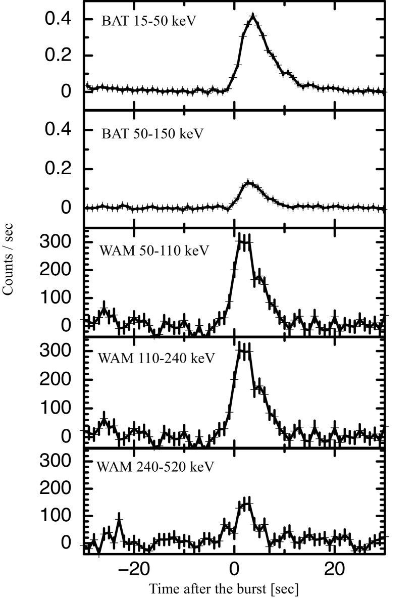
Figure 1: Prompt $\gamma$-ray light curves observed by Swift/BAT and Suzaku/WAM. The trigger time of Swift/BAT is used as T₀.

The Suzaku/WAM also triggered the burst at 01:20:31.9 (T${}_{0}+2.9$ s) UT on March 26, 2012. The WAM (Yamaoka et al., 2009) is a lateral shield of the Hard X-ray Detector (Takahashi et al., 2007) on board the Suzaku satellite (Mitsuda et al., 2007) and is a powerful GRB spectrometer covering an energy range of 50$-$5000 keV to determine prompt spectral energy peaks $E_{peak}$ (e.g., Ohno et al., 2008; Tashiro et al., 2007; Urata et al., 2009). As shown in Figure 1, the prompt X-ray and $\gamma$-ray light curves observed using the Swift/BAT and Suzaku/WAM exhibited a single fast-rise-exponential-decay (FRED) structure.

We performed the optical afterglow observations using the Lulin One-meter Telescope (Huang et al., 2005) and the LOAO robotic 1-m telescope (Han et al., 2005; Lee et al., 2010) within the framework of the EAFON (Urata et al., 2003). Four color observations were made with LOT on the night of March 26. The LOAO data were obtained in $R$ band filter from 2013 March 26 to April 2. The afterglow was also observed with Camera for Quasars in Early Universe (Camera for QUasars in the EArly uNiverse; Park et al., 2012; Kim et al., 2011; Lim et al., 2013) on the 2.1-m Otto-Struve telescope of the McDonald observatory, Texas, USA. The data were obtained in $g,r,i,z$, and $Y$ filters, starting at 2013 March 26, 10:09:22 (UT), and continued till April 2. The logs for both observations are summarized in Table 1.

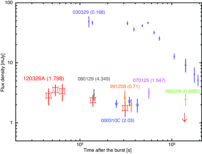
Figure 2: Light curves of all the submm afterglows detected in 230 GHz band to date. The SMA observation on GRB120326A provides the earliest submm detection and continuous monitoring. The values noted in brackets is redshift of each event. The samples are taken from Galama et al. (2000) for 991208, Berger et al. (2000) for 0000301C, Resmi et al. (2005); Sheth et al. (2003) for 030329, Chandra et al. (2008) for 070125, Gorosabel et al. (2010) for 080109, and Greiner et al. (2009) for 080129.

We also triggered the submm continuum follow-up observations by using the seven 6-m antennas of SMA (Ho et al., 2004). The first continuum observation at 230 GHz (with an 8 GHz bandwidth) was conducted at 10:15:05 on March 26, 2012, about $4.6\times 10^{4}$ s after the BAT trigger. As Urata et al. (2012) reported, the submm counterpart was observed at the location of the X-ray and optical afterglow. The continuous monitoring using the SMA was also performed at the same frequency setting on March 27, 29, 31, and April 6, and 11. Table 2 summarizes the scientific observations that were conducted for 4 nights, because of weather conditions and antenna reconfiguration. Figure 2 shows submm light curves of all the GRB afterglows detected at the 230 GHz to date. Among all seven events, we successfully detected the earliest submm afterglow on GRB120326A. A possible reason for this successful submm monitoring was the target selection using the quick optical follow-ups.

3 Analysis and Results

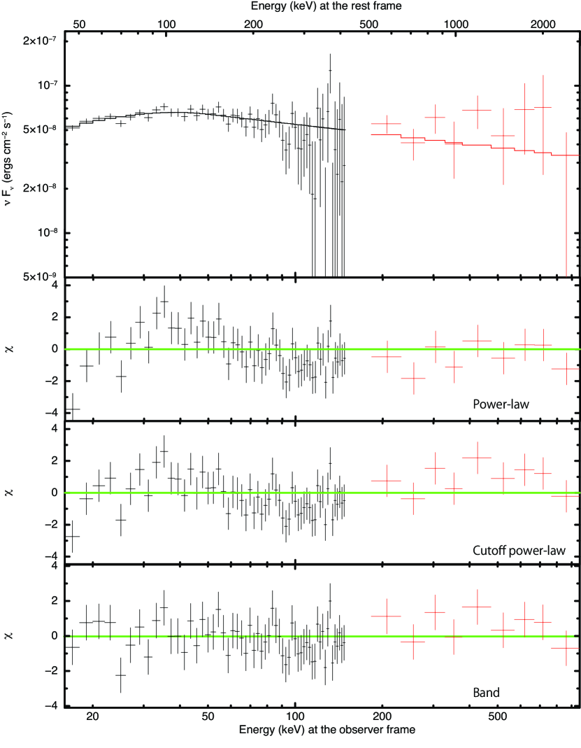
Figure 3: Time-averaged spectrum of the prompt emission, observed using Swift/BAT and Suzaku/WAM. The BAT and WAM data are shown in black and red colros, respectively. In the top panel, the solid lines indicate the best-fit Band function model. The lower panels show residuals for fitting with power-law (2nd), power-law with exponential cutoff (3rd), and Band (4th) models.

The BAT data were analyzed using the standard BAT analysis software included in HEADAS v6.12. The time averaged spectrum (15 – 150 keV) from T${}_{0}-2$ to T${}_{0}+11$ s was extracted using batgrbproduct. Response matrices were generated by the task batdrmgen, using the latest spectral redistribution matrices. The WAM spectral and temporal data were extracted using hxdmkwamlc and hxdmkwamspec in HEADAS version 6.12. The background was estimated using the fitting model described in Sugita et al. (2009). Response matrices were generated by the WAM response generator as described in Ohno et al. (2008). We used three models for the joint spectral fitting: power-law, power-law with exponential cutoff, and Band function model. As shown in Figure 3, the spectrum was reasonably fitted with the Band function. The fitting yielded a low-energy photon index of $1.17^{+0.53}_{-0.32}$, high-energy photon index of $2.23^{+0.09}_{-0.11}$ and $\nu F\nu$ spectrum peak energy in the source frame $E^{\rm src}_{\rm peak}$ of $107.8^{+15.2}_{-15.3}$ keV ($\chi^{2}/\nu=0.92$ for $\nu=63$). Both power-law ($\chi^{2}/\nu=1.55$ for $\nu=65$) and power-law with exponential cutoff ($\chi^{2}/\nu=1.38$ for $\nu=67$) were not acceptable, leaving a curvature of the residuals around 30-40 keV at the observer frame (the 2nd and 3rd panele in Figure 3). We also estimated the equivalent isotropic radiated energy in the prompt phase at the 1-10000keV band $\rm E_{\rm iso}$ as $3.18^{+0.40}_{-0.32}\times 10^{52}$ erg, assuming cosmological parameters: $H_{0}=71{\rm km/s/Mpc}$, $\Omega_{m}=0.27$, and $\Omega_{\Lambda}=0.73$.

We obtained a reduced Swift/XRT light curve with a flux density unit at 10 keV from the U.K. Swift Science Data Center (Evans et al., 2007, 2009). The light curves shown in Figure 4 were suitably fitted using the broken power-law model described in (Urata et al., 2009), using the best fitted parameters of $\alpha_{X1}=0.19\pm 0.09$, $\alpha_{X2}=-2.35\pm 0.15$, and $t_{bX}=(5.29\pm 0.32)\times 10^{4}$ s. We also generated the time-averaged spectrum at a mean time of $6.47\times 10^{4}$ s (from 55741 to 73639 s). The spectra were suitably fitted using power-law modified by photo-electric absorptions (galactic and intrinsic), and the photon index was estimated as $1.95^{+0.18}_{-0.17}$.

A standard routine including bias subtraction and flat-fielding corrections was employed to processes the optical data by using the IRAF package. The DAOPHOT package was used to perform aperture photometry of the GRB images. Standard star observation in one night is used to derive magnitudes of reference stars in the vicinity of the GRB afterglow, and these reference stars were used to perform photometry of the afterglow. We also made use of the Pan-STARRS1 $3\pi$ catalogs (Magnier et al., 2013; Schlafly et al., 2012; Tonry et al., 2012) to calibrate our $g^{\prime}$, $r^{\prime}$, $i^{\prime}$, $z^{\prime}$, and $Y$ band data. As shown in Figure 4, the light curves in the $g^{\prime}$, $r^{\prime}$, $i^{\prime}$, and $z^{\prime}$ bands indicated the achromatic temporal break at $\sim 2.6\times 10^{5}$ s. We successfully fitted the broken power-law model to the $g^{\prime}$, $r^{\prime}$, $i^{\prime}$, and $z^{\prime}$ bands light curves. Regarding the $g^{\prime}$ band, we have obtained $\alpha_{g1}=-1.01\pm 0.06$, $\alpha_{g2}=-2.84\pm 0.16$, and $t_{bg}=(2.58\pm 0.15)\times 10^{5}$ s; regarding the $r^{\prime}$ band, $\alpha_{r1}=-0.96\pm 0.01$, $\alpha_{r2}=-2.64\pm 0.09$, and $t_{br}=(2.58\pm 0.07)\times 10^{5}$ s; regarding the $i^{\prime}$ band, $\alpha_{i1}=-0.88\pm 0.02$, $\alpha_{i2}=-2.48\pm 0.05$, and $t_{bi}=(2.51\pm 0.10)\times 10^{5}$ s; regarding the $z^{\prime}$ band, $\alpha_{z1}=-0.89\pm 0.01$, $\alpha_{z2}=-2.64\pm 0.10$, and $t_{bz}=(2.63\pm 0.06)\times 10^{5}$ s; and regarding the $y^{\prime}$ band, we fitted the light curve by using the simple power-law model, because the $y^{\prime}$ band observations covered only before the temporal break. The light curve was fitted with the model and we obtained $\alpha_{y}=-0.87\pm 0.03$. The decay indices before and after the break are $\sim-1$ and $\sim-2$, respectively, which is highly consistent with typical well-observed long GRB optical afterglows. In Figure 5, we plot the spectral flux distribution with the submm and X-ray data. We fitted the optical data alone using a power-law function and obtained $\beta=-1.44\pm 0.10$, $-1.11\pm 0.09$, and $-1.18\pm 0.17$ at $t=6.42\times 10^{4}$ s, $1.38\times 10^{5}$ s, and $3.10\times 10^{5}$ s, respectively. To remove the effects of the Galactic interstellar extinction, we used the reddening map by Schlafly & Finkbeiner (2011).

The raw data of the SMA observations were calibrated using the MIR and MIRIAD packages and images were made with the natural weighting. Regarding the first night of observation, we split the data into three periods to describe the temporal evolution of submm afterglow. Table 2 summarizes each observation period and flux density measurements (upper part). Because of adverse weather conditions during the first $1.08\times 10^{4}$ s, only the data recorded after 13:00 on March 26 UT were used for the scientific analysis. In the final period, we constrained the 3$\sigma$ upper limit. With our SMA follow-ups, we successfully monitored the afterglow from $4.32\times 10^{4}$ to $3.46\times 10^{5}$ s as shown in Figure 4. The submm afterglow exhibited a flat evolution with slight brightening between the first and second periods. To describe the temporal evolution, we fitted the submm data with the single power-law function and obtained $\alpha_{\rm submm}=-0.33\pm 0.08$, which was considerably flatter than those of the X-ray and optical.

4 Discussion

4.1 Prompt Emission and Energetics Relations

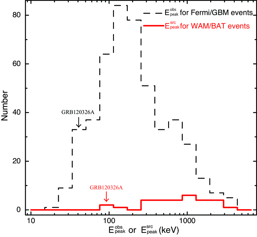
Figure 6: The distribution of $E^{\rm src}_{\rm peak}$ for BAT/WAM events and $E^{\rm obs}_{\rm peak}$ for Fermi /GBM events. GRB120326A is one of the lowest $E^{\rm src}_{\rm peak}$ events among the BAT/WAM sample. $E^{\rm obs}_{\rm peak}$ also shows the same trend with large Fermi /GBM samples; although the measurements was analyzed without redshift correction.

The joint fitting of the Swift/BAT and Suzaku/WAM suitably constrained the spectral parameters of the prompt emission of GRB120326A that are critical to characterize event. As shown in Figure 6, the spectral peak energy in the source frame $E^{\rm src}_{peak}$ is one of the lowest events among the sample of the joint Swift/BAT-Suzaku/WAM analysis. The trend is similar to that of the $\nu F\nu$ spectral peak energy at the observer frame $E^{obs}_{peak}$ in comparison to a larger set of $E^{obs}_{peak}$ values of 479 GRBs drawn from the Fermi /GBM catalog von Kienlin et al. (2014); although, the Fermi /GBM measurements do not represent $E^{\rm src}_{peak}$ due to the lack of redshift information. By comparing with the HETE-2 sample (Sakamoto et al., 2005), GRB120326A can be categorized as X-ray rich GRBs. Using the definition with Swift/BAT data (Sakamoto et al., 2008), we confirm that GRB120326A with $\sim 0.74$ fluence ratio in the 25-50 keV and 50-100 keV bands falls into the X-ray rich GRB family.

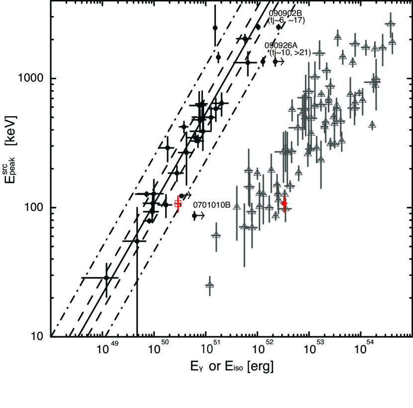
Figure 7: The $E^{\rm src}_{\rm peak}-E_{\rm iso}$ relation in Amati et al. (2002) (open triangle) and the $E^{\rm src}_{\rm peak}-E_{\rm\gamma}$ relation corrected for a homogeneous circumburst medium (filled circle). GRB120326A marked with red box points obeyed both relations. The solid line indicates the best fit correlation derived by Ghirlanda et al. (2007). The dashed and dash-dotted lines indicate the 1$\sigma$ and 3$\sigma$ scatter of the correlation, respectively.

The abundance of the multi-color optical light curves for estimating the jet break time suggests that GRB120326A is a favorable target for evaluating ${E^{\rm src}_{\rm peak}-E_{\rm iso}}$(Amati et al., 2002) and ${E^{\rm src}_{\rm peak}-E_{\rm\gamma}}$(Ghirlanda et al., 2007) relations. Here, ${E^{\rm src}_{\rm peak}-E_{\rm\gamma}}$ is the correlation between the intrinsic spectrum peak energy ${E^{\rm src}_{\rm peak}}$ and the jet collimation-corrected energy in the prompt phase, ${E_{\rm\gamma}}$. The closure relation of the observed optical temporal decay and the spectral indices (e.g., Sari et al., 1999; Zhang & Mészáros, 2004) indicates that, of all the $p>2$ options, the optical results are consistent with both the fast and the slow cooling and both the wind and the ISM medium, as long as $\nu_{m,FS}$ and $\nu_{c,FS}$ lie below the optical band. Here, $\nu_{m,FS}$ and $\nu_{c,FS}$ are the characteristic synchrotron frequency and the cooling frequency based on the standard forward shock synchrotron model. Thus, the jet opening angle and the jet corrected energy are estimated using $t_{br}$ as $6^{\circ}.69\pm 0^{\circ}.16$ and $(2.17\pm 0.10)\times 10^{50}$ erg by assuming the circumburst density $n=$1.0 ${\rm cm^{-3}}$ and the energy conversion efficiency $\eta_{\gamma}=0.2$, To covert the measured jet break time $t_{br}$ to the jet opening angle, we used the formulation of Sari et al. (1999) and Frail et al. (2001). As shown in Figure 7, GRB120326A obeys the ${E^{\rm src}_{\rm peak}-E_{\rm iso}}$ and ${E^{\rm src}_{\rm peak}-E_{\rm\gamma}}$ relations within $3\sigma$ confidence level. Therefore, GRB120326A belongs to the typical long duration GRB family, even with a low $E^{\rm src}_{peak}$.

4.2 Does Classical Forward Shock Synchrotorn model work?

Based on the closure relations, the observed temporal evolution and spectral features of the optical afterglow are well consistent with those of the forward shock synchrotron model. The fact that $\nu_{m,FS}$ and $\nu_{c,FS}$ both lie below the optical band, implies that within the standard synchrotron model, X-ray afterglow therefore lie in the same spectral regime as the optical emission, and that the standard model therefore predicts the same temporal and spectral shape for X-rays as for the optical.

However, the observed X-ray light curve shows a significant deviation from the predicted behavior of the standard model and appears to require an additional component. Using the testing method of the forward shock model using the decay index ($\alpha{\rm o}-\alpha_{X}$) relation between the optical and X-ray(Urata et al., 2007), we find that GRB120326A is a clear outlier ($\alpha{\rm o}-\alpha_{X}=-1.45\pm 0.10$) and the origin of the X-ray afterglow could differ from that of the optical. For conducting a more rigorous analysis, we selected the normal optical decay phase as from $3.2\times 10^{4}$ s to $2.1\times 10^{5}$ s. The optical light curve in this phase is well fitted with a simple power law function with an index of $-0.96\pm 0.01$. For the time range, we forced to fit the X-ray light curve with the simple power law function and obtained the decay index of $-1.54\pm 0.14$. Hence, this event remained outlier ($\alpha{\rm o}-\alpha_{X}=-0.58\pm 0.14$) and the X-ray emission could have a extra component such as X-ray flare on the forward shock synchrotron emission.

To check the excess in the X-ray light curve, we shifted optical light curve to the X-ray band with the factor $(\nu_{X}/\nu_{opt})^{-p/2}$ by assuming the X-ray and optical lie on the same segment of the synchrotron radiation. We used $p=2.48$ with $3\sigma$ error of 0.15 estimated from the optical observations and the closure relation. As shown in Figure 4, the shifted light curve shows a significant gap with that of observed X-ray and the gap is rather smaller after $\sim 3\times 10^{5}$ s. One of the main reasons of the gap is no consideration of the intrinsic extinction for the optical component at the burst site due to lack of spectral coverage in the optical observations. If the main X-ray component after $3\times 10^{5}$ is originated from the same segment of forward shock synchrotron radiation with optical (as sharing the similr decay index with those of optical), $A_{V}=0.3\sim 0.5$ mag with the SMC extinction curve is required to fill up the smaller gap after the $3\times 10^{5}$ s. The extinction value of $A_{V}=0.3\sim 0.5$ mag is rather larger comparing with other majority of optically bright events ($A_{V}<0.25$ mag) (Kann et al., 2006, 2010). We also added the shifted optical light curve with $p=2$ that provides the upper limit of the forward shock synchrotron radiation under the $p>2$ condition (Figure 4. Although these imply that adjustment of $p$ and introducing extinction may be the solution to explain the gap after $3\times 10^{5}$, there remains a significant X-ray excess between $2\times 10^{4}$ and $3\times 10^{5}$ s.

The forward shock synchrotorn model based on the optical afterglow is also impossible to explain the submm emission. Based on the closure relation, the slow decay observed in the submm light curve requirs $\nu_{c,FS}<\nu_{submm}<\nu_{m,FS}$ (i.e. fast cooling condition for both ISM and wind types). Hence, $\nu_{c,FS}<\nu_{submm}<\nu_{m,FS}<\nu_{opt}$ is required to satisfy the closure relation for the submm and optical afterglows all together. In addition to the closure relation, the observed flux densities (both in the submm and optical bands) at $6.42\times 10^{4}$ s and the temporal decay index in the optical bands tightly constrain the range of characterized frequencies as $\nu_{c,FS}<2.3\times 10^{11}$ Hz and $\nu_{m,FS}\sim 3\times 10^{14}$ Hz to make the fast cooling condition. With these conditions, we find that even a drastic case (e.g. $\epsilon_{B}\sim 1$ and $\epsilon_{e}\sim 1$ with very high density of $n>$ several $\times 10^{3}$ cm^-3) cannot meet the condition and that the origin of submm component also could differ from that of the optical. Thus, additional radiation is required to explain X-ray and submm emissions all together.

4.3 Foward Shock Synchrotron modeling

To describe the entire spectral energy distribution, we performed modeling for the optical light curves and spectra by using the boxfit code (van Eerten et al., 2012) that involved two-dimensional relativistic hydrodynamical jet simulations to determine the burst explosion and the synchrotron radiation parameters with a homogeneous circumburst medium. Hence, hereafter, we only consider the ISM condition and do not verify whether ISM or wind condition is favorable. This code also performs data fitting with the downhill simplex method combined with simulated annealing. Based on the observational results, we fixed as $\theta_{jet}=6^{\circ}.7$ and a power-law electron spectrum of slope $p=2.5$. The observing angle was also fixed as $\theta_{obs}=0$. By using only the optical data with the code, we determined the optimal modeling parameters to describe the optical light curves as $E=3.9\times 10^{52}$ erg, $n=1.0$ cm^-3, $\epsilon_{B}=1.0\times 10^{-3}$, and $\epsilon_{e}=6.9\times 10^{-1}$. To adjust the model function, we also set the jet opening angle as a free parameter and then $\theta_{jet}=8.1^{\circ}$ provided favorable agreement ($\chi^{2}/\nu=3.9$ for $\nu=94$) with observing the light curve. The solid line in Figure 4 indicates the best model function for the $r^{\prime}$ band light curve, which also well agreed with the analytical model function. This opening angle adjustment is reasonable because $\theta_{jet}=6^{\circ}.7$ was estimated by considering the conical jet. Additional note is that the post jet-break closure relation is no longer valid under the consideration of detailed spreading of the jet (van Eerten & MacFadyen, 2013). However, we are not concerned about this, since we were able to achieve the good fit with the simulation-based fit models. With the adjusted jet opening angle, GRB120326A still obeyed the ${E^{\rm src}_{\rm peak}-E_{\rm\gamma}}$ relation. We also attempted to determine the optimal solution by using optical and submm data with the code. However, no sufficient solution describe the temporal evolution of submm and optical afterglow all together was determined by the $\chi^{2}$ evaluation with $2.3\times 10^{4}$ iterations. All of trials provided reduced $\chi^{2}$ greater than 13. This is consistent with the forward shock testings described above. We generated the forward shock synchrotron model spectrum by using the box fit with the best modeling parameters for the light curve. Figure 5 shows the SED at $6.42\times 10^{4}$ s after the burst. The spectrum in the X-ray and submm exhibited substantial excesses from the best model function and indicated that the afterglow spectrum required additional radiation components. This interpretation is also consistent with the result of the $\alpha{o}-\alpha_{X}$ relation and the shifted optical light curve to the X-ray band with factor $(\nu_{X}/\nu_{opt})^{-p/2}$.

4.4 Reverse Shock and Synchrotron Self-Compton

A solution that explains the X-ray excess and the different origin of the submm emission is to introduce synchrotron self-inverse Compton radiation from reverse shock. This is one of the most feasible method to deal two notable observed properties all together. Assuming the deceleration time is near the X-ray light curve peak at $t_{bX}\sim 5.2\times 10^{4}$ s, the initial Lorentz factor $\Gamma_{0}$ is estimated as $\sim 16$, which is consistent with the thin-shell case ($\Gamma_{c}\sim 365$). Here, $\Gamma_{c}$ is the critical Lorentz factor that distinguishes thin shell models where the reverse shock remains Newtonian, from thick shell models (Sari & Piran, 1995; Kobayashi et al., 2007). This lower $\Gamma_{0}$ might be associated with the low $E^{src}_{peak}$ property. It might also originate from the cocoon fireball as part of two-component jet in the collapsar framework (e.g., Ramirez-Ruiz et al., 2002). In this case, thermal radiation is expected to arise in the optical light curves (Kashiyama et al., 2013; Nakauchi et al., 2013). However, the observed optical light curves show no excess in the late phase.

Using the estimated parameters described in above, we calculated the model function for synchrotron self-inverse Compton radiation from reverse shock under the thin-shell condition described in Kobayashi et al. (2007). For this calculation, we assumed $\epsilon_{B,RS}\sim 5\times 10^{-3}$, and peak flux densities of reverse and forward shocks as $F_{max,RS}\sim 5.5$ mJy and $F_{max,FS}\sim 0.2$ mJy, respectively. Figure 5 shows the calculated spectrum for the reverse shock and inverse Compton components at $6.42\times 10^{4}$ s with the obtained key parameters of $\nu^{Sync}_{m,RS}\sim 4\times 10^{11}{\rm Hz}$, $\nu^{Sync}_{c,RS}\sim 7\times 10^{12}{\rm Hz}$, $\nu^{IC}_{m,RS}\sim 1\times 10^{17}{\rm Hz}$, and $\nu^{IC}_{c,RS}\sim 4\times 10^{19}{\rm Hz}$. Although the observed X-ray flux was slightly brighter than calculated self-inverse Compton component, the total spectrum including forward shock was sufficiently described the overall properties of the afterglow. Because $\nu_{obs}<\nu^{Sync}_{m,RS}$, the expected decay index of the reverse shock component in the observed submm band was $\sim-0.46$, which was consistent with the slow temporal evolution of the submm afterglow ($\alpha_{submm}=-0.33$). The relatively shallower evolution than that of expected also implies the smooth transition of $\nu^{Sync}_{m,RS}$ in the observing band, unlike the sharp break in Figure 4. This could be same with other spectrum break such as non-existence of sharp cooling break in afterglow spectrum (e.g., Granot & Sari, 2002; van Eerten & Wijers, 2009; Curran et al., 2010). The observed X-ray decay ($\alpha_{X}\sim-2.4$) and spectrum ($\beta_{X}\sim-0.96$) indices were also basically consistent with the expected values ($\alpha_{X}\sim$2.8 and $\beta_{X}\sim-0.75$) for $\nu^{IC}_{m,RS}<\nu_{obs}<\nu^{IC}_{c,RS}$.

5 Summary

We conducted multi-wavelength observations of a typical long duration GRB 120326A, including rapid observations using SMA. Our SMA observation successfully made the fastest afterglow detection among seven submm afterglows at 230 GHz, and monitored from $4.32\times 10^{4}$ to $3.46\times 10^{5}$ s. The submm afterglow showed considerably slower temporal evolution ($\alpha_{submm}=-0.33\pm 0.08$) which is unlikely to be explained by the forward shock synchrotron model. Based on our dense optical observations, we presented the optical afterglows were well fitted by the broken power-law model and the forward shock synchrotron model is feasible to explain the properties. With the boxfit code, we also found the reasonable model function within the forward shock synchrotron model under the assumption of ISM circumburst medium. Using the simple testing method of the forward shock model with temporal decay indices of optical and X-ray afterglows, we found the origin of the X-ray afterglow could differ from that of optical. Our joint spectrum fitting for prompt emission using Swift/BAT and Suzaku/WAM also characterized the event and find that current event obey the ${E^{\rm src}_{\rm peak}-E_{\rm iso}}$ and ${E^{\rm src}_{\rm peak}-E_{\rm\gamma}}$ relations with in $3\sigma$ confidence level.

Based on the detection and the slow decay of the afterglow in submm, we introduced the synchrotron self-inverse Compton radiation from reverse shock and find that this is a plausible idea to explain the diversity. This successful modeling could benefit other GRBs. Similar to GRB120326A, numerous events exhibited no apparent jet breaks in X-ray band and different temporal evolutions between the X-ray and optical. These observational properties imply that additional component such as reverse shock and its synchrotron self-inverse Compton radiation make the different temporal evolution and hide obvious jet break in X-ray. Because of a lack of submm observations for these samples, interpretation from the same picture for these events was difficult. Thus, further rapid follow-ups and continuous monitoring with submm instruments such as SMA and Atacama Large Millimeter/submillimeter Array (ALMA) will enable systematic testing of the reverse shock and self-inverse Compton radiation.

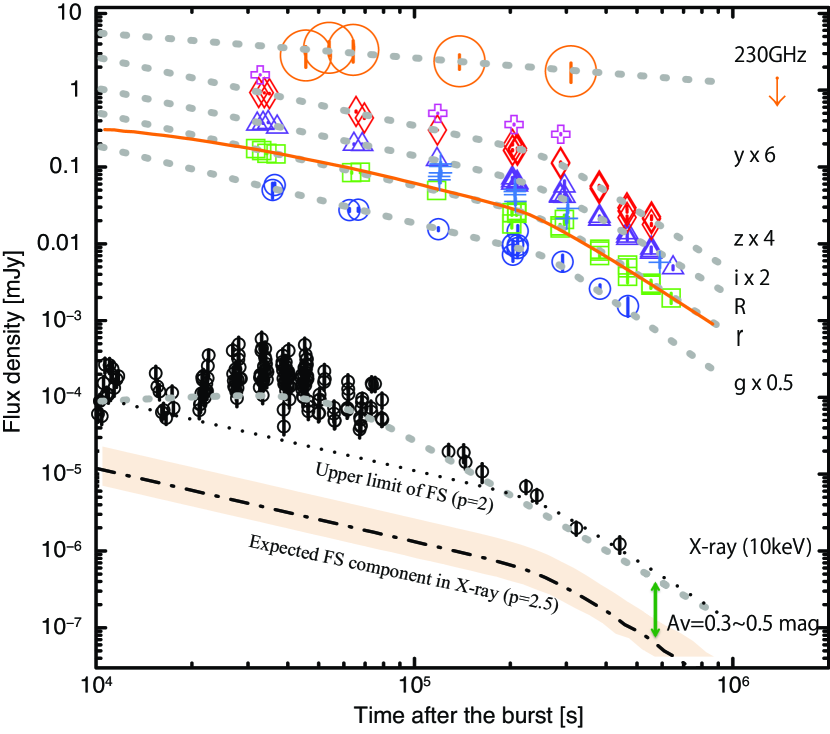
Figure 4: X-ray, optical and submm light curves of the GRB120326A afterglow. The grey dotted lines show the best analytical fitted functions described in the text. The orange solid line shows the best modeling function for the $r$-band light curve obtained with the numerical simulation using boxfit. The black dash-dotted and dotted lines indicat the shifted optical light curve to the X-ray bands by factor of $(\nu_{X}/\nu_{opt})^{-p/2}$ with $p=2.5$ and $p=2$, respectively.

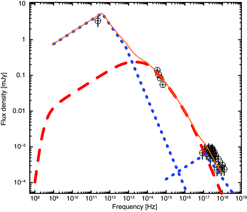
Figure 5: The spectral energy distribution at $6.42\times 10^{4}$ s after the burst. The red dashed line shows the forward shock synchrotron model spectrum calculated using the boxfit code with the same parameters for the best modeling light curve shown in left panel. The blue dotted lines show the reverse shock synchrotron radiation and its self-inverse Compton component calculated based on Kobayashi et al. (2007) using the observed values and model function for the forward shock component.

Table 1: Log of optical observations.

Instruments	T-T0 (s)	Filter	Exposure (s)	Flux density (mJy)
CQUEAN	35818	$g$	120	$(5.031\pm 1.114)\times 10^{-2}$
CQUEAN	36428	$g$	120	$(5.843\pm 0.364)\times 10^{-2}$
LOT	62495	$g$	300	$(2.751\pm 0.130)\times 10^{-2}$
LOT	66550	$g$	300	$(2.781\pm 0.132)\times 10^{-2}$
CQUEAN	118878	$g$	120	$(1.549\pm 0.072)\times 10^{-2}$
CQUEAN	203667	$g$	120	$(9.670\pm 1.290)\times 10^{-3}$
CQUEAN	203788	$g$	120	$(7.200\pm 1.310)\times 10^{-3}$
CQUEAN	203909	$g$	120	$(9.820\pm 1.150)\times 10^{-3}$
CQUEAN	210775	$g$	120	$(8.840\pm 2.050)\times 10^{-3}$
CQUEAN	210896	$g$	120	$(9.580\pm 2.540)\times 10^{-3}$
CQUEAN	211018	$g$	120	$(1.460\pm 0.271)\times 10^{-2}$
CQUEAN	291923	$g$	120$\times$5	$(5.800\pm 1.330)\times 10^{-3}$
CQUEAN	382503	$g$	300$\times$3	$(2.600\pm 0.320)\times 10^{-3}$
CQUEAN	468068	$g$	300$\times$3	$(1.550\pm 0.420)\times 10^{-3}$
LOAO	119527	$R$	300	$(7.517\pm 0.848)\times 10^{-2}$
LOAO	119845	$R$	300	$(6.792\pm 0.654)\times 10^{-2}$
LOAO	120163	$R$	300	$(8.395\pm 0.596)\times 10^{-2}$
LOAO	120532	$R$	300	$(1.019\pm 0.055)\times 10^{-1}$
LOAO	120882	$R$	300	$(1.096\pm 0.059)\times 10^{-1}$
LOAO	121197	$R$	300	$(8.395\pm 0.596)\times 10^{-2}$
LOAO	206539	$R$	300	$(4.787\pm 0.579)\times 10^{-2}$
LOAO	206865	$R$	300	$(4.365\pm 0.633)\times 10^{-2}$
LOAO	207181	$R$	300	$(5.105\pm 0.740)\times 10^{-2}$
LOAO	207498	$R$	300	$(3.565\pm 0.373)\times 10^{-2}$
LOAO	301087	$R$	900	$(2.148\pm 0.242)\times 10^{-2}$
LOAO	300315	$R$	900	$(2.128\pm 0.275)\times 10^{-2}$
LOAO	303167	$R$	1200	$(2.884\pm 0.349)\times 10^{-2}$
LOAO	589749	$R$	2700	$(5.750\pm 0.880)\times 10^{-3}$
CQUEAN	31732	$r$	300	$(1.734\pm 0.022)\times 10^{-1}$
CQUEAN	33129	$r$	300	$(1.636\pm 0.008)\times 10^{-1}$
CQUEAN	34399	$r$	300	$(1.510\pm 0.027)\times 10^{-1}$
CQUEAN	36739	$r$	300	$(1.478\pm 0.010)\times 10^{-1}$
LOT	63503	$r$	300	$(8.434\pm 0.177)\times 10^{-2}$
LOT	67564	$r$	300	$(8.591\pm 0.165)\times 10^{-2}$
CQUEAN	117385	$r$	300	$(4.955\pm 0.036)\times 10^{-2}$
CQUEAN	202218	$r$	120	$(1.812\pm 0.207)\times 10^{-2}$
CQUEAN	202340	$r$	120	$(2.526\pm 0.175)\times 10^{-2}$
CQUEAN	202461	$r$	120	$(2.544\pm 0.141)\times 10^{-2}$
CQUEAN	209219	$r$	120	$(2.586\pm 0.236)\times 10^{-2}$
CQUEAN	209633	$r$	120	$(2.720\pm 0.116)\times 10^{-2}$
CQUEAN	209754	$r$	120	$(2.496\pm 0.119)\times 10^{-2}$
CQUEAN	286528	$r$	120	$(1.715\pm 0.075)\times 10^{-2}$
CQUEAN	286650	$r$	120	$(1.712\pm 0.067)\times 10^{-2}$
CQUEAN	286771	$r$	120	$(1.603\pm 0.065)\times 10^{-2}$
CQUEAN	295768	$r$	120	$(2.072\pm 0.291)\times 10^{-2}$
CQUEAN	381506	$r$	180	$(8.050\pm 0.380)\times 10^{-3}$
CQUEAN	381688	$r$	180	$(7.040\pm 0.390)\times 10^{-3}$
CQUEAN	381869	$r$	180	$(8.500\pm 0.380)\times 10^{-3}$
CQUEAN	466726	$r$	300	$(5.300\pm 0.710)\times 10^{-3}$
CQUEAN	467028	$r$	300	$(3.770\pm 0.670)\times 10^{-3}$
CQUEAN	467329	$r$	300	$(4.860\pm 0.550)\times 10^{-3}$
CQUEAN	552707	$r$	300	$(2.890\pm 0.270)\times 10^{-3}$
CQUEAN	553009	$r$	300	$(2.930\pm 0.290)\times 10^{-3}$
CQUEAN	553310	$r$	300	$(3.070\pm 0.300)\times 10^{-3}$
CQUEAN	639867	$r$	300$\times$6	$(1.970\pm 0.300)\times 10^{-3}$
CQUEAN	32074	$i$	300	$(3.621\pm 0.010)\times 10^{-1}$
CQUEAN	33448	$i$	300	$(3.701\pm 0.005)\times 10^{-1}$
CQUEAN	34711	$i$	300	$(3.803\pm 0.023)\times 10^{-1}$
CQUEAN	37050	$i$	300	$(3.311\pm 0.039)\times 10^{-1}$
LOT	68583	$i$	300	$(1.964\pm 0.028)\times 10^{-1}$
LOT	64510	$i$	300	$(1.982\pm 0.021)\times 10^{-1}$
CQUEAN	117705	$i$	300	$(1.257\pm 0.003)\times 10^{-1}$
CQUEAN	202624	$i$	120	$(6.634\pm 0.084)\times 10^{-2}$
CQUEAN	202746	$i$	120	$(6.164\pm 0.082)\times 10^{-2}$
CQUEAN	202867	$i$	120	$(7.226\pm 0.084)\times 10^{-2}$
CQUEAN	209979	$i$	120	$(5.834\pm 0.089)\times 10^{-2}$
CQUEAN	210100	$i$	120	$(6.346\pm 0.102)\times 10^{-2}$
CQUEAN	210222	$i$	120	$(6.188\pm 0.103)\times 10^{-2}$
CQUEAN	286927	$i$	120	$(4.194\pm 0.069)\times 10^{-2}$
CQUEAN	287048	$i$	120	$(4.292\pm 0.099)\times 10^{-2}$
CQUEAN	287169	$i$	120	$(4.360\pm 0.071)\times 10^{-2}$
CQUEAN	287313	$i$	120	$(4.186\pm 0.063)\times 10^{-2}$
CQUEAN	295903	$i$	120	$(4.150\pm 0.235)\times 10^{-2}$
CQUEAN	296025	$i$	120	$(5.662\pm 0.943)\times 10^{-2}$
CQUEAN	380844	$i$	180	$(2.118\pm 0.036)\times 10^{-2}$
CQUEAN	381025	$i$	180	$(2.092\pm 0.038)\times 10^{-2}$
CQUEAN	381206	$i$	180	$(2.278\pm 0.036)\times 10^{-2}$
CQUEAN	465783	$i$	300	$(1.256\pm 0.056)\times 10^{-2}$
CQUEAN	466084	$i$	300	$(1.178\pm 0.060)\times 10^{-2}$
CQUEAN	466386	$i$	300	$(1.390\pm 0.057)\times 10^{-2}$
CQUEAN	553652	$i$	300	$(7.760\pm 0.280)\times 10^{-3}$
CQUEAN	553954	$i$	300	$(8.820\pm 0.280)\times 10^{-3}$
CQUEAN	554255	$i$	300	$(8.200\pm 0.270)\times 10^{-3}$
CQUEAN	648922	$i$	300$\times$6	$(4.880\pm 0.290)\times 10^{-3}$
CQUEAN	32416	$z$	300	$(9.325\pm 0.016)\times 10^{-1}$
CQUEAN	33766	$z$	300	$(9.250\pm 0.021)\times 10^{-1}$
CQUEAN	35023	$z$	300	$(9.018\pm 0.073)\times 10^{-1}$
LOT	65534	$z$	300	$(5.278\pm 0.088)\times 10^{-1}$
LOT	69604	$z$	300	$(4.358\pm 0.085)\times 10^{-1}$
CQUEAN	118015	$z$	300	$(3.025\pm 0.006)\times 10^{-1}$
CQUEAN	203042	$z$	120	$(1.639\pm 0.020)\times 10^{-1}$
CQUEAN	203163	$z$	120	$(1.970\pm 0.032)\times 10^{-1}$
CQUEAN	203285	$z$	120	$(1.660\pm 0.024)\times 10^{-1}$
CQUEAN	210347	$z$	120	$(1.744\pm 0.018)\times 10^{-1}$
CQUEAN	210468	$z$	120	$(1.650\pm 0.018)\times 10^{-1}$
CQUEAN	210589	$z$	120	$(1.744\pm 0.019)\times 10^{-1}$
CQUEAN	287478	$z$	120	$(1.113\pm 0.017)\times 10^{-1}$
CQUEAN	287600	$z$	120	$(1.112\pm 0.017)\times 10^{-1}$
CQUEAN	287721	$z$	120	$(1.147\pm 0.016)\times 10^{-1}$
CQUEAN	380256	$z$	120	$(5.236\pm 0.079)\times 10^{-2}$
CQUEAN	380438	$z$	120	$(5.696\pm 0.083)\times 10^{-2}$
CQUEAN	380619	$z$	120	$(5.524\pm 0.078)\times 10^{-2}$
CQUEAN	464838	$z$	180	$(2.944\pm 0.141)\times 10^{-2}$
CQUEAN	465140	$z$	180	$(2.680\pm 0.103)\times 10^{-2}$
CQUEAN	465441	$z$	180	$(2.204\pm 0.100)\times 10^{-2}$
CQUEAN	554653	$z$	300	$(1.784\pm 0.060)\times 10^{-2}$
CQUEAN	554955	$z$	300	$(2.248\pm 0.062)\times 10^{-2}$
CQUEAN	555256	$z$	300	$(2.120\pm 0.064)\times 10^{-2}$
CQUEAN	32776	$Y$	300	$1.585\pm 0.004$
CQUEAN	118338	$Y$	300	$(5.005\pm 0.025)\times 10^{-1}$
CQUEAN	205445	$Y$	120$\times$6	$(3.576\pm 0.054)\times 10^{-1}$
CQUEAN	288007	$Y$	120$\times$3	$(2.672\pm 0.053)\times 10^{-1}$

Table 2: Log of SMA observations.

Instruments	Observing period (UT)	T-T0 (s)	Band (GHz)	Beam size	Flux density (mJy)
SMA	2012-03-26 13:00-15:00	45571	230	$1".74\times 1".14$	2.84 $\pm$ 0.86
SMA	2012-03-26 15:10-17:30	53971	230	$1".69\times 1".02$	3.56 $\pm$ 0.75
SMA	2012-03-26 18:00-20:15	64171	230	$2".03\times 0".96$	3.36 $\pm$ 1.04
SMA	2012-03-27 13:25-19:15	138480	230	$1".62\times 1".11$	2.38 $\pm$ 0.51
SMA	2012-03-29 12:45-18:50	310290	230	$0".62\times 0".37$	1.76 $\pm$ 0.50
SMA	2012-04-11 15:50-21:10	1377571	230	$0".55\times 0".42$	$<1.44(3\sigma)$

References

- Akerlof et al. (1999) Akerlof, C., Balsano, R., Barthelmy, S., et al. 1999, Nature, 398, 400
- Amati et al. (2002) Amati, L., et al. 2002, A&A, 390, 81
- Berger et al. (2000) Berger, E., Sari, R., Frail, D. A., et al. 2000, ApJ, 545, 56
- Chandra et al. (2008) Chandra, P., Cenko, S. B., Frail, D. A., et al. 2008, ApJ, 683, 924
- Chandara&Frail (2012) Chandra & Frail 2012, ApJ, 746, 156
- Collazzi (2012) Collazzi, A. C. 2012, GRB Coordinates Network, 13145, 1
- Curran et al. (2010) Curran, P. A., Evans, P. A., de Pasquale, M., Page, M. J., & van der Horst, A. J. 2010, ApJ, 716, L135
- de Ugarte Postigo et al. (2012) de Ugarte Postigo, A., Lundgren, A., Martín, S., et al. 2012, A&A, 538, A44
- Evans et al. (2009) Evans, P. A., Beardmore, A. P., Page, K. L., et al. 2009, MNRAS, 397, 1177
- Evans et al. (2007) Evans, P. A., Beardmore, A. P., Page, K. L., et al. 2007, A&A, 469, 379
- Frail et al. (2001) Frail, D. A., Kulkarni, S. R., Sari, R., et al. 2001, ApJ, 562, L55
- Galama et al. (2000) Galama, T. J., Bremer, M., Bertoldi, F., et al. 2000, ApJ, 541, L45
- Granot & Sari (2002) Granot, J., & Sari, R. 2002, ApJ, 568, 820
- Gehrels et al. (2004) Gehrels, N., Chincarini, G., Giommi, P., et al. 2004, ApJ, 611, 1005
- Ghirlanda et al. (2007) Ghirlanda, G., Nava, L., Ghisellini, G., and Firmani, G., 2007, å, 466, 127
- Gorosabel et al. (2010) Gorosabel, J., de Ugarte Postigo, A., Castro-Tirado, A. J., et al. 2010, A&A, 522, A14
- Greiner et al. (2009) Greiner, J., Krühler, T., McBreen, S., et al. 2009, ApJ, 693, 1912
- Han et al. (2005) Han, W., et al. 2005, PASJ, 57, 821
- Ho et al. (2004) Ho, P. T. P., Moran, J. M., & Lo, K. Y. 2004, ApJ, 616, L1
- Huang et al. (2007) Huang, K. Y., Urata, Y., Kuo, P. H., et al. 2007, ApJ, 654, L25
- Huang et al. (2005) Huang, K. Y., Urata, Y., Filippenko, A. V., et al. 2005, ApJ, 628, L93
- Iwakiri et al. (2012) Iwakiri, W., Tashiro, M., Terada, Y., et al. 2012, GRB Coordinates Network, 13176, 1
- Laskar et al. (2012) Laskar, T., Zauderer, A., & Berger, E. 2012, GRB Coordinates Network, 13181, 1
- Lee et al. (2010) Lee, I., Im, M., & Urata, Y. 2010, Journal of Korean Astronomical Society, 43, 95
- Li et al. (2012) Li, L., Liang, E.-W., Tang, Q.-W., et al. 2012, ApJ, 758, 27
- Lim et al. (2013) Lim, J., Chang, S., Pak, S., et al. 2013, Journal of Korean Astronomical Society, 46, 161
- Kann et al. (2010) Kann, D. A., Klose, S., Zhang, B., et al. 2010, ApJ, 720, 1513
- Kann et al. (2006) Kann, D. A., Klose, S., & Zeh, A. 2006, ApJ, 641, 993
- Kashiyama et al. (2013) Kashiyama, K., Nakauchi, D., Suwa, Y., Yajima, H., & Nakamura, T. 2013, ApJ, 770, 8
- Klotz et al. (2012) Klotz, A., Gendre, B., Boer, M., & Atteia, J. L. 2012, GRB Coordinates Network, 13107, 1
- Kim et al. (2011) Kim, E., Park, W.-K., Jeong, H., et al. 2011, Journal of Korean Astronomical Society, 44, 115
- Kobayashi et al. (2007) Kobayashi, S., Zhang, B., Mészáros, P., & Burrows, D. 2007, ApJ, 655, 391
- Kulkarni et al. (1999) Kulkarni, S. R., Frail, D. A., Sari, R., et al. 1999, ApJ, 522, L97
- Magnier et al. (2013) Magnier, E. A., Schlafly, E., Finkbeiner, D., et al. 2013, ApJS, 205, 20
- Meszaros & Rees (1997) Meszaros, P., & Rees, M. J. 1997, ApJ, 476, 232
- Mitsuda et al. (2007) Mitsuda, K., et al. 2007, PASJ, 59, 1
- Nakauchi et al. (2013) Nakauchi, D., Kashiyama, K., Suwa, Y., & Nakamura, T. 2013, ApJ, 778, 67
- Oates et al. (2011) Oates, S. R., Page, M. J., Schady, P., et al. 2011, MNRAS, 412, 561
- Ohno et al. (2008) Ohno, M., et al. 2008, PASJ, 60, 361
- Panaitescu & Vestrand (2011) Panaitescu, A., & Vestrand, W. T. 2011, MNRAS, 414, 3537
- Panaitescu et al. (2006) Panaitescu, A., Mészáros, P., Burrows, D., et al. 2006, MNRAS, 369, 2059
- Park et al. (2012) Park, W.-K., Pak, S., Im, M., et al. 2012, PASP, 124, 839
- Perley et al. (2012) Perley, D. A., Alatalo, K., & Horesh, A. 2012, GRB Coordinates Network, 13175, 1
- Ramirez-Ruiz et al. (2002) Ramirez-Ruiz, E., Celotti, A., & Rees, M. J. 2002, MNRAS, 337, 1349
- Resmi et al. (2005) Resmi, L., Ishwara-Chandra, C. H., Castro-Tirado, A. J., et al. 2005, A&A, 440, 477
- Sakamoto et al. (2005) Sakamoto, T., Lamb, D. Q., Kawai, N., et al. 2005, ApJ, 629, 311
- Sakamoto et al. (2008) Sakamoto, T., Hullinger, D., Sato, G., et al. 2008, ApJ, 679, 570
- Sari & Piran (1995) Sari, R., & Piran, T. 1995, ApJ, 455, L143
- Sari et al. (1999) Sari, R., Piran, T., & Halpern, J. P. 1999, ApJ, 519, L17
- Schlafly et al. (2012) Schlafly, E. F., Finkbeiner, D. P., Jurić, M., et al. 2012, ApJ, 756, 158
- Schlafly & Finkbeiner (2011) Schlafly, E. F., & Finkbeiner, D. P. 2011, ApJ, 737, 103
- Sheth et al. (2003) Sheth, K., Frail, D. A., White, S., et al. 2003, ApJ, 595, L33
- Siegel et al. (2012) Siegel, M. H., Barthelmy, S. D., Burrows, D. N., et al. 2012, GRB Coordinates Network, 13105, 1
- Sugita et al. (2009) Sugita, S., et al. 2009, PASJ, Vol. 61, No. 3, pp. 521–527
- Takahashi et al. (2007) Takahashi, T., et al. 2007, PASJ, 59, 35
- Tashiro et al. (2007) Tashiro, M. S., Abe, K., Angelini, L., et al. 2007, PASJ, 59, 361
- Tello et al. (2012) Tello, J. C., Sanchez-Ramirez, R., Gorosabel, J., et al. 2012, GRB Coordinates Network, 13118, 1
- Tonry et al. (2012) Tonry, J. L., Stubbs, C. W., Lykke, K. R., et al. 2012, ApJ, 750, 99
- Toma et al. (2008) Toma, K., Ioka, K., & Nakamura, T. 2008, ApJ, 673, L123
- Uhm & Zhang (2013) Uhm, Z. L., & Zhang, B. 2013, arXiv:1301.0291
- Urata et al. (2012) Urata, Y., Huang, K. Y., Takahashi, S., & Petitpas, G. 2012, GRB Coordinates Network, 13136, 1
- Urata et al. (2009) Urata, Y., et al. 2009, ApJ, 706, L183
- Urata et al. (2007) Urata, Y., et al. 2007, ApJ, 668, L95
- Urata et al. (2003) Urata, Y., et al. 2003, ApJ, 595, L21
- van Eerten & MacFadyen (2013) van Eerten, H., & MacFadyen, A. 2013, ApJ, 767, 141
- van Eerten et al. (2012) van Eerten, H., van der Horst, A., & MacFadyen, A. 2012, ApJ, 749, 44
- van Eerten & Wijers (2009) van Eerten, H. J., & Wijers, R. A. M. J. 2009, MNRAS, 394, 2164
- von Kienlin et al. (2014) von Kienlin, A., Meegan, C. A., Paciesas, W. S., et al. 2014, ApJS, 211, 13
- Walker et al. (2012) Walker, C., Court, J., Duffy, R., et al. 2012, GRB Coordinates Network, 13112, 1
- Yamaoka et al. (2009) Yamaoka, K.., et al. 2009, PASJ, 61, S35
- Zhang & Mészáros (2004) Zhang, B., & Mészáros, P. 2004, International Journal of Modern Physics A, 19, 2385