IFT-UAM/CSIC-14-018

FTUAM-14-016

Imprints of massive inverse seesaw model neutrinos in lepton flavor violating Higgs boson decays

E. Arganda1***ernesto.arganda@unizar.es, M.J. Herrero2maria.herrero@uam.es, X. Marcano2xabier.marcano@uam.es, C. Weiland2§§§cedric.weiland@uam.es

1Departamento de Física Teórica, Facultad de Ciencias,
Universidad de Zaragoza, E-50009 Zaragoza, Spain

2Departamento de Física Teórica and Instituto de Física Teórica, IFT-UAM/CSIC,
Universidad Autónoma de Madrid, Cantoblanco, 28049 Madrid, Spain

Abstract

In this paper we consider a Higgs boson with mass and other properties compatible with those of the recently discovered Higgs particle at the LHC, and explore the possibility of new Higgs leptonic decays, beyond the standard model, with the singular feature of being lepton flavor violating (LFV). We study these LFV Higgs decays, Hlkl¯m𝐻subscript𝑙𝑘subscript¯𝑙𝑚H\to l_{k}\bar{l}_{m}, within the context of the inverse seesaw model (ISS) and consider the most generic case where three additional pairs of massive right-handed singlet neutrinos are added to the standard model particle content. We require in addition that the input parameters of this ISS model are compatible with the present neutrino data and other constraints, like perturbativity of the neutrino Yukawa couplings. We present a full one-loop computation of the BR(Hlkl¯m𝐻subscript𝑙𝑘subscript¯𝑙𝑚H\to l_{k}\bar{l}_{m}) rates for the three possible channels, lkl¯m=μτ¯,eτ¯,eμ¯subscript𝑙𝑘subscript¯𝑙𝑚𝜇¯𝜏𝑒¯𝜏𝑒¯𝜇l_{k}\bar{l}_{m}=\mu\bar{\tau},\,e\bar{\tau},\,e\bar{\mu}, and analyze in full detail the predictions as functions of the various relevant ISS parameters. We study in parallel the correlated one-loop predictions for the radiative decays, lmlkγsubscript𝑙𝑚subscript𝑙𝑘𝛾l_{m}\to l_{k}\gamma, within this same ISS context, and require full compatibility of our predictions with the present experimental bounds for the three radiative decays, μeγ𝜇𝑒𝛾\mu\to e\gamma, τμγ𝜏𝜇𝛾\tau\to\mu\gamma, and τeγ𝜏𝑒𝛾\tau\to e\gamma. After exploring the ISS parameter space we conclude on the maximum allowed LFV Higgs decay rates within the ISS.

1 Introduction

At present, there seems to be a broad consensus in the high energy physics community that the recently discovered scalar particle at the CERN-LHC [1, 2] behaves as the Higgs particle of the standard model of particle physics (SM). The most recent measurements of this scalar particle mass by the ATLAS and CMS collaborations set mhATLAS=125.5±0.6superscriptsubscript𝑚ATLASplus-or-minus125.50.6m_{h}^{\rm ATLAS}=125.5\pm 0.6 GeV [3] and mhCMS=125.7±0.4superscriptsubscript𝑚CMSplus-or-minus125.70.4m_{h}^{\rm CMS}=125.7\pm 0.4 GeV [4], respectively. These experiments also show that the most probable JPsuperscript𝐽𝑃J^{P} quantum numbers for this discovered Higgs boson are 0+superscript00^{+}, and conclude that the measured Higgs particle couplings to the other SM particles are in agreement so far, although yet with moderate precision, with the values predicted in the SM. Also the scalar Higgs-like particle width ΓhsubscriptΓ\Gamma_{h} has been found to be Γh<17.4subscriptΓ17.4\Gamma_{h}<17.4 MeV which is about 4.2 times the SM value [5].

On the other hand, there is also a major consensus that the SM must be modified in order to include the neutrino masses and oscillations in agreement with present data, which are nowadays quite impressive and urge of an explanation from a theoretical framework beyond the SM. Thus, in order to be compatible with the present neutrino data we choose here to go beyond the SM using one of its simplest and more appealing extensions, the inverse seesaw model (ISS) [6, 7, 8]. This ISS extends the SM particle content by adding pairs of right-handed (RH) neutrinos with opposite lepton number whose masses and couplings can be properly chosen to produce the physical light neutrino masses and oscillations in good agreement with present data [9, 10, 11]. In contrast to the original seesaw type I model [12, 13, 14, 15, 16], the seesaw mechanism that produces the small light physical neutrino masses in the ISS is associated to the smallness of the Majorana mass model parameters, such that when these are set to zero lepton number conservation is restored, therefore increasing the symmetries of the model. Another appealing feature of the ISS is that it allows for large Yukawa neutrino couplings while having at the same time moderately heavy right-handed neutrino masses at the 𝒪(TeV)𝒪TeV{\cal O}({\rm TeV}) energies that are reachable at the present colliders, like the LHC. In addition to the possibility of being directly produced at colliders, these right-handed neutrinos could also lead to a new rich phenomenology in connection with lepton flavor violating (LFV) Physics. This is because the ISS right-handed neutrinos can produce non-negligible contributions to LFV processes via radiative corrections that are mediated by the sizable neutrino Yukawa couplings, therefore leading to clear signals/imprints in these rare processes, which are totally absent in the SM . These LFV processes include the most frequently studied radiative decays, μeγ𝜇𝑒𝛾\mu\to e\gamma, τμγ𝜏𝜇𝛾\tau\to\mu\gamma, τeγ𝜏𝑒𝛾\tau\to e\gamma, others like μ3e𝜇3𝑒\mu\to 3e, leptonic and semileptonic τ𝜏\tau decays, μe𝜇𝑒\mu-e conversion in heavy nuclei, and others (see [17] for a review). The ISS mechanism also has implications on deviations from lepton flavor universality [18, 19] and from lepton number conservation [20, 21, 22, 23, 24]. Although quite promising future sensitivities for some of these LFV processes are expected, for instance, for μe𝜇𝑒\mu-e conversion in heavy nuclei [26, 27, 28, 25], at present the highest sensitivity to LFV signals is obtained in μeγ𝜇𝑒𝛾\mu\to e\gamma where MEG has set an upper bound at branching ratio (BR), BR(μeγ)<5.7×10¹³𝜇𝑒𝛾5.7superscript1013(\mu\to e\gamma)<5.7\times 10^{-13} [29].

In this paper, we study other LFV processes, the Higgs decays into lepton-antilepton pairs Hlkl¯m𝐻subscript𝑙𝑘subscript¯𝑙𝑚H\to l_{k}\bar{l}_{m} with km𝑘𝑚k\neq m, which are of obvious interest at present, given the recent discovery of the Higgs particle and the fact that these rare Higgs decays are also being presently explored at the LHC. The current direct search at the LHC for these LFV Higgs decays (LFVHD) has been recently reported in [30], where an upper limit of BR(Hμτ)<1.57%𝐻𝜇𝜏percent1.57(H\to\mu\tau)<1.57\% at 95%percent9595\% C.L. has been set using 19.7fb119.7superscriptfb119.7~{}\mathrm{fb}^{-1} of s=8𝑠8\sqrt{s}=8 TeV. This improves previous constraints from indirect measurements at LHC [31] by roughly one order of magnitude (see also [32]), and it is close to the previous estimates in [33] that predicted sensitivities of 4.5×1034.5superscript1034.5\times 10^{-3} (see also, [34]). The future perspectives for LFVHD searches are encouraging due to the expected high statistics of Higgs events at future hadronic and leptonic colliders. Although, to our knowledge, there is no realistic study, including background estimates, of the expected future experimental sensitivities for these kinds of rare LFVHD events, a naive extrapolation from the present situation can be done. For instance, the future LHC runs with s=14𝑠14\sqrt{s}=14 TeV and total integrated luminosity of first 300fb1300superscriptfb1300~{}\rm{fb}^{-1} and later 3000fb13000superscriptfb13000~{}\rm{fb}^{-1} expect the production of about 25 and 250 million Higgs events, respectively, to be compared with 1 million Higgs events that the LHC produced after the first run [35]. These large numbers suggest an improvement in the long-term sensitivities to BR(Hμτ)𝐻𝜇𝜏(H\to\mu\tau) of at least two orders of magnitude with respect to the present sensitivity. Similarly, at the planned lepton colliders, like the international linear collider (ILC) with111We thank J. Fuster for private communication with the updated ILC perspectives. s=1𝑠1\sqrt{s}=1 TeV and 2.5ab12.5superscriptab12.5~{}\rm{ab}^{-1}[36], and the future electron-positron circular collider (FCC-ee) as the TLEP with s=350𝑠350\sqrt{s}=350 GeV and 10ab110superscriptab110~{}\rm{ab}^{-1}[37], the expectations are of about 1 and 2 million Higgs events, respectively, with much lower backgrounds due to the cleaner environment, which will also allow for a large improvement in LFV Higgs searches with respect to the current sensitivities.

We will present a full one-loop computation of the LFV partial decay widths, Γ(Hlkl¯m)Γ𝐻subscript𝑙𝑘subscript¯𝑙𝑚\Gamma(H\to l_{k}\bar{l}_{m}), within the ISS context with three extra pairs of right-handed neutrinos, and will analyze in full detail the predictions for the LFVHD rates, BR(Hlkl¯m)𝐻subscript𝑙𝑘subscript¯𝑙𝑚(H\to l_{k}\bar{l}_{m}), as functions of the various relevant ISS parameters. These LFV Higgs decays were analyzed in the context of the SM enlarged with three heavy Majorana neutrinos for the first time in [38]. Later, they were computed in the context of the seesaw I model in [39], and they were found to lead to extremely small rates due to the strong suppression from the extremely heavy right-handed neutrino masses, at 101415superscript10141510^{14-15} GeV, in that case. This motivates our study of the LFV Higgs decays in the ISS case with the right-handed neutrino masses lying in contrast at the 𝒪(TeV)𝒪TeV{\cal O}({\rm TeV}) energy scale and therefore the rates are expected to be larger than in the seesaw I case. The interest of neutrino masses at this 𝒪(TeV)𝒪TeV\mathcal{O}(\rm{TeV}) energy scale is also because they can be directly produced at the LHC. Furthermore, we will also study in parallel the correlated one-loop predictions for the radiative decays, BR(lmlkγsubscript𝑙𝑚subscript𝑙𝑘𝛾l_{m}\to l_{k}\gamma), within this same ISS context, and we will require full compatibility of our predictions with the present experimental upper bounds for the three relevant radiative decays, μeγ𝜇𝑒𝛾\mu\to e\gamma, τμγ𝜏𝜇𝛾\tau\to\mu\gamma, and τeγ𝜏𝑒𝛾\tau\to e\gamma, the first one being the most constraining one. We will require in addition that the input parameters of the ISS are compatible with the present neutrino data and other constraints, like perturbativity of the neutrino Yukawa couplings. After exploring the ISS parameter space we will conclude on the maximum allowed LFV Higgs decay rates within the ISS.

The paper is organized as follows: in section 2 we summarize our theoretical framework and shortly review the main features of the ISS that are relevant for the present computation. In section 3 we present our computation of the one-loop LFV Higgs decay widths within the ISS and include, for completeness and comparison, both the analytical formulas for the LFV Higgs decays and the LFV radiative decays. The full one-loop analytical formulas for the LFV Higgs form factors are collected in the Appendix. Section 4 is devoted to the presentation of the numerical results of our computation and also includes the predictions for both kind of LFV processes, the branching ratios for the LFV Higgs decays, Hμτ¯𝐻𝜇¯𝜏H\to\mu\bar{\tau}, Heτ¯𝐻𝑒¯𝜏H\to e\bar{\tau}, and Heμ¯𝐻𝑒¯𝜇H\to e\bar{\mu} that we compare with the branching ratios for the radiative decays, τμγ𝜏𝜇𝛾\tau\to\mu\gamma, τeγ𝜏𝑒𝛾\tau\to e\gamma, and μeγ𝜇𝑒𝛾\mu\to e\gamma. Finally, we summarize our conclusions in section 5.

2 Theoretical framework

One of the simplest extensions of the SM leading to nonzero neutrino masses and mixing is the addition of fermionic gauge singlets. As mentioned above, a very attractive model is the ISS that supplements the SM with pairs of RH neutrinos, denoted here by νRsubscript𝜈𝑅\nu_{R} and X𝑋X, with opposite lepton number. While the minimal model that fits oscillation data requires only two generations of RH neutrinos [40], we consider here a more generic model containing three pairs of fermionic singlets. It extends the SM Lagrangian with the following neutrino Yukawa interactions and mass terms:

ISS=YνijLi¯Φ~νRjMRijνRiC¯Xj12μXijXiC¯Xj+h.c.,formulae-sequencesubscriptISSsubscriptsuperscript𝑌𝑖𝑗𝜈¯subscript𝐿𝑖~Φsubscript𝜈𝑅𝑗superscriptsubscript𝑀𝑅𝑖𝑗¯superscriptsubscript𝜈𝑅𝑖𝐶subscript𝑋𝑗12superscriptsubscript𝜇𝑋𝑖𝑗¯superscriptsubscript𝑋𝑖𝐶subscript𝑋𝑗𝑐\mathcal{L}_{\mathrm{ISS}}=-Y^{ij}_{\nu}\overline{L_{i}}\widetilde{\Phi}\nu_{Rj}-M_{R}^{ij}\overline{\nu_{Ri}^{C}}X_{j}-\frac{1}{2}\mu_{X}^{ij}\overline{X_{i}^{C}}X_{j}+h.c.\,, (1)

where L𝐿L is the SM lepton doublet, ΦΦ\Phi is the SM Higgs doublet, Φ~=ıσ2Φ~Φitalic-ısubscript𝜎2superscriptΦ\widetilde{\Phi}=\imath\sigma_{2}\Phi^{*}, with σ2subscript𝜎2\sigma_{2} being the corresponding Pauli matrix, Yνsubscript𝑌𝜈Y_{\nu} is the 3×3333\times 3 neutrino Yukawa coupling matrix, MRsubscript𝑀𝑅M_{R} is a lepton number conserving complex 3×3333\times 3 mass matrix, and μXsubscript𝜇𝑋\mu_{X} is a Majorana complex 3×3333\times 3 symmetric mass matrix that violates lepton number conservation by two units. Setting the latter to zero would restore the conservation of lepton number, thus increasing the symmetry of the model. This makes the smallness of μXsubscript𝜇𝑋\mu_{X} natural since it could be seen as the remnant of a symmetry broken at a higher energy [41]. Since a Majorana mass term of the type νRi¯νRjC¯subscript𝜈𝑅𝑖superscriptsubscript𝜈𝑅𝑗𝐶\overline{\nu_{Ri}}\nu_{Rj}^{C} would only give subleading corrections to the neutrino masses and the observables considered here, we have taken it to be zero, for simplicity.

After electroweak symmetry breaking, the 9×9999\times 9 neutrino mass matrix reads, in the electroweak interaction basis (νLC,νR,X)superscriptsubscript𝜈𝐿𝐶subscript𝜈𝑅𝑋(\nu_{L}^{C}\,,\;\nu_{R}\,,\;X),

MISS=(0mD0mDT0MR0MRTμX),subscript𝑀ISS0subscript𝑚𝐷0superscriptsubscript𝑚𝐷𝑇0subscript𝑀𝑅0superscriptsubscript𝑀𝑅𝑇subscript𝜇𝑋M_{\mathrm{ISS}}=\left(\begin{array}[]{c c c}0&m_{D}&0\\ m_{D}^{T}&0&M_{R}\\ 0&M_{R}^{T}&\mu_{X}\end{array}\right)\,, (2)

with the 3×3333\times 3 Dirac mass matrix given by mD=YνΦsubscript𝑚𝐷subscript𝑌𝜈delimited-⟨⟩Φm_{D}=Y_{\nu}\langle\Phi\rangle, and the Higgs vacuum expectation value is taken to be Φ=v=174GeVdelimited-⟨⟩Φ𝑣174GeV\langle\Phi\rangle=v=174\,\mathrm{GeV}. Since this mass matrix is complex and symmetric, it can be diagonalized using a 9×9999\times 9 unitary matrix Uνsubscript𝑈𝜈U_{\nu} according to

UνTMISSUν=diag(mn1,,mn9).subscriptsuperscript𝑈𝑇𝜈subscript𝑀ISSsubscript𝑈𝜈diagsubscript𝑚subscript𝑛1subscript𝑚subscript𝑛9U^{T}_{\nu}M_{\mathrm{ISS}}U_{\nu}=\text{diag}(m_{n_{1}},\dots,m_{n_{9}})\,. (3)

This gives three light mass eigenstates and six heavy mass eigenstates, and the electroweak eigenstates and the mass eigenstates are related through

(νLCνRX)=UνPR(n1n9),(νLνRCXC)=UνPL(n1n9).\left(\begin{array}[]{c}\nu_{L}^{C}\\ \nu_{R}\\ X\end{array}\right)=U_{\nu}P_{R}\left(\begin{array}[]{c}n_{1}\\ \vdots\\ n_{9}\end{array}\right)\,\quad,\quad\left(\begin{array}[]{c}\nu_{L}\\ \nu_{R}^{C}\\ X^{C}\end{array}\right)=U_{\nu}^{*}P_{L}\left(\begin{array}[]{c}n_{1}\\ \vdots\\ n_{9}\end{array}\right)\,. (4)

In order to illustrate more simply the dependence on the seesaw parameters, let us first consider the one generation case and then we will come back to the three generation case. In this one generation case there are just three ISS model parameters, MRsubscript𝑀𝑅M_{R}, μXsubscript𝜇𝑋\mu_{X}, and Yνsubscript𝑌𝜈Y_{\nu}, and there are just three physical eigenstates: one light ν𝜈\nu and two heavy N1subscript𝑁1N_{1} and N2subscript𝑁2N_{2}. In the limit μXmD,MRmuch-less-thansubscript𝜇𝑋subscript𝑚𝐷subscript𝑀𝑅\mu_{X}\ll m_{D},M_{R}, the mass eigenvalues are given by:

mνsubscript𝑚𝜈\displaystyle m_{\nu} =mD2mD2+MR2μX,absentsuperscriptsubscript𝑚𝐷2superscriptsubscript𝑚𝐷2superscriptsubscript𝑀𝑅2subscript𝜇𝑋\displaystyle=\frac{m_{D}^{2}}{m_{D}^{2}+M_{R}^{2}}\mu_{X}\,, (5)
mN1,N2subscript𝑚subscript𝑁1subscript𝑁2\displaystyle m_{N_{1},N_{2}} =±MR2+mD2+MR2μX2(mD2+MR2),absentplus-or-minussuperscriptsubscript𝑀𝑅2superscriptsubscript𝑚𝐷2superscriptsubscript𝑀𝑅2subscript𝜇𝑋2superscriptsubscript𝑚𝐷2superscriptsubscript𝑀𝑅2\displaystyle=\pm\sqrt{M_{R}^{2}+m_{D}^{2}}+\frac{M_{R}^{2}\mu_{X}}{2(m_{D}^{2}+M_{R}^{2})}\,, (6)

with the light neutrino mass mνsubscript𝑚𝜈m_{\nu} being proportional to μXsubscript𝜇𝑋\mu_{X}, thus making it naturally small, and the two heavy masses mN1,N2subscript𝑚subscript𝑁1subscript𝑁2m_{N_{1},N_{2}} being close to each other. As a consequence in this μXmD,MRmuch-less-thansubscript𝜇𝑋subscript𝑚𝐷subscript𝑀𝑅\mu_{X}\ll m_{D},M_{R} limit, these two nearly degenerate heavy neutrinos combine to form pseudo-Dirac fermions.

A similar pattern of neutrino mass eigenvalues occurs in the three generation case, with one light and two nearly degenerate heavy neutrinos per generation. This can be illustrated clearly in the limit μXmDMRmuch-less-thansubscript𝜇𝑋subscript𝑚𝐷much-less-thansubscript𝑀𝑅\mu_{X}\ll m_{D}\ll M_{R}, where the mass matrix MISSsubscript𝑀ISSM_{\mathrm{ISS}} can be diagonalized by blocks [42], leading to the following 3×3333\times 3 light neutrino mass matrix:

MlightmDMRT1μXMR1mDT,similar-to-or-equalssubscript𝑀lightsubscript𝑚𝐷superscriptsuperscriptsubscript𝑀𝑅𝑇1subscript𝜇𝑋superscriptsubscript𝑀𝑅1superscriptsubscript𝑚𝐷𝑇M_{\mathrm{light}}\simeq m_{D}{M_{R}^{T}}^{-1}\mu_{X}M_{R}^{-1}m_{D}^{T}\,, (7)

which is then diagonalized using the unitary Pontecorvo–-Maki-–Nakagawa–-Sakata (PMNS) matrix UPMNSsubscript𝑈PMNSU_{\rm PMNS}[43]:

UPMNSTMlightUPMNS=diag(mν1,mν2,mν3),superscriptsubscript𝑈PMNS𝑇subscript𝑀lightsubscript𝑈PMNSdiagsubscript𝑚subscript𝜈1subscript𝑚subscript𝜈2subscript𝑚subscript𝜈3U_{\rm PMNS}^{T}M_{\mathrm{light}}U_{\rm PMNS}=\mathrm{diag}(m_{\nu_{1}}\,,m_{\nu_{2}}\,,m_{\nu_{3}})\,, (8)

where mν1subscript𝑚subscript𝜈1m_{\nu_{1}}, mν2subscript𝑚subscript𝜈2m_{\nu_{2}}, and mν3subscript𝑚subscript𝜈3m_{\nu_{3}} are the masses of the three lightest neutrinos.

Then, by defining a new 3×3333\times 3 mass matrix by

M=MRμX1MRT,𝑀subscript𝑀𝑅superscriptsubscript𝜇𝑋1superscriptsubscript𝑀𝑅𝑇M=M_{R}\mu_{X}^{-1}M_{R}^{T}, (9)

the light neutrino mass matrix can be written similarly to the type I seesaw model as:

MlightmDM1mDT.similar-to-or-equalssubscript𝑀lightsubscript𝑚𝐷superscript𝑀1superscriptsubscript𝑚𝐷𝑇M_{\mathrm{light}}\simeq m_{D}M^{-1}m_{D}^{T}\,. (10)

The mass pattern of the heavy neutrinos in the μXmDMRmuch-less-thansubscript𝜇𝑋subscript𝑚𝐷much-less-thansubscript𝑀𝑅\mu_{X}\ll m_{D}\ll M_{R} limit presents a similar behavior to the one generation case. The heavy neutrinos form quasidegenerate pairs with a mass approximately given by the eigenvalues of MRsubscript𝑀𝑅M_{R}, namely MR1,2,3subscript𝑀subscript𝑅123M_{R_{1,2,3}} for the first, second, and third generation, respectively, and with a splitting of order 𝒪(μX)𝒪subscript𝜇𝑋\mathcal{O}(\mu_{X}).

For our phenomenological purposes, and in order to implement easily the compatibility with present neutrino data, we will use here the useful Casas-Ibarra parametrization [44] that can be directly applied to the inverse seesaw model case, giving

mDT=Vdiag(M1,M2,M3)Rdiag(mν1,mν2,mν3)UPMNS,superscriptsubscript𝑚𝐷𝑇superscript𝑉diagsubscript𝑀1subscript𝑀2subscript𝑀3𝑅diagsubscript𝑚subscript𝜈1subscript𝑚subscript𝜈2subscript𝑚subscript𝜈3subscriptsuperscript𝑈PMNSm_{D}^{T}=V^{\dagger}\mathrm{diag}(\sqrt{M_{1}}\,,\sqrt{M_{2}}\,,\sqrt{M_{3}})\;R\;\mathrm{diag}(\sqrt{m_{\nu_{1}}}\,,\sqrt{m_{\nu_{2}}}\,,\sqrt{m_{\nu_{3}}})U^{\dagger}_{\rm PMNS}\,, (11)

where V𝑉V is a unitary matrix that diagonalizes M𝑀M according to M=Vdiag(M1,M2,M3)V𝑀superscript𝑉diagsubscript𝑀1subscript𝑀2subscript𝑀3superscript𝑉M=V^{\dagger}\mathrm{diag}(M_{1}\,,M_{2}\,,M_{3})V^{*} and R𝑅R is a complex orthogonal matrix that can be written as

R=(c2c3c1s3s1s2c3s1s3c1s2c3c2s3c1c3s1s2s3s1c3c1s2s3s2s1c2c1c2),𝑅subscript𝑐2subscript𝑐3subscript𝑐1subscript𝑠3subscript𝑠1subscript𝑠2subscript𝑐3subscript𝑠1subscript𝑠3subscript𝑐1subscript𝑠2subscript𝑐3subscript𝑐2subscript𝑠3subscript𝑐1subscript𝑐3subscript𝑠1subscript𝑠2subscript𝑠3subscript𝑠1subscript𝑐3subscript𝑐1subscript𝑠2subscript𝑠3subscript𝑠2subscript𝑠1subscript𝑐2subscript𝑐1subscript𝑐2R=\left(\begin{array}[]{ccc}c_{2}c_{3}&-c_{1}s_{3}-s_{1}s_{2}c_{3}&s_{1}s_{3}-c_{1}s_{2}c_{3}\\ c_{2}s_{3}&c_{1}c_{3}-s_{1}s_{2}s_{3}&-s_{1}c_{3}-c_{1}s_{2}s_{3}\\ s_{2}&s_{1}c_{2}&c_{1}c_{2}\end{array}\right)\,, (12)

where cicosθisubscript𝑐𝑖subscript𝜃𝑖c_{i}\equiv\cos\theta_{i}, sisinθisubscript𝑠𝑖subscript𝜃𝑖s_{i}\equiv\sin\theta_{i} and θ1subscript𝜃1\theta_{1}, θ2subscript𝜃2\theta_{2}, and θ3subscript𝜃3\theta_{3} are arbitrary complex angles.

In summary, assuming μX=diag(μX1,μX2,μX3)subscript𝜇𝑋diagsubscript𝜇subscript𝑋1subscript𝜇subscript𝑋2subscript𝜇subscript𝑋3\mu_{X}={\rm diag}(\mu_{X_{1}},\mu_{X_{2}},\mu_{X_{3}}) and MR=diag(MR1,MR2,MR3)subscript𝑀𝑅diagsubscript𝑀subscript𝑅1subscript𝑀subscript𝑅2subscript𝑀subscript𝑅3M_{R}={\rm diag}(M_{R_{1}},M_{R_{2}},M_{R_{3}}) (hence, diagonal M𝑀M), the input ISS parameters that will have to be fixed for our forthcoming study of the LFV rates are the following: mν1,2,3subscript𝑚subscript𝜈123m_{\nu_{1,2,3}}, μX1,2,3subscript𝜇subscript𝑋123\mu_{X_{1,2,3}}, MR1,2,3subscript𝑀subscript𝑅123M_{R_{1,2,3}}, θ1,2,3subscript𝜃123\theta_{1,2,3}, and the entries of the UPMNSsubscript𝑈PMNSU_{\rm PMNS} matrix. For all the numerical analysis in this work, and in order to keep agreement with the experimental neutrino data, we will choose the lightest neutrino mass, here assumed to be mν1subscript𝑚subscript𝜈1m_{\nu_{1}}, as a free input parameter and the other two light masses will be obtained from the two experimentally measured mass differences:

mν2=mν12+Δm212,mν3=mν12+Δm312.formulae-sequencesubscript𝑚subscript𝜈2superscriptsubscript𝑚subscript𝜈12Δsuperscriptsubscript𝑚212subscript𝑚subscript𝜈3superscriptsubscript𝑚subscript𝜈12Δsuperscriptsubscript𝑚312m_{\nu_{2}}=\sqrt{m_{\nu_{1}}^{2}+\Delta m_{21}^{2}}\ ,\quad m_{\nu_{3}}=\sqrt{m_{\nu_{1}}^{2}+\Delta m_{31}^{2}}\ . (13)

Similarly, the three light neutrino mixing angles will also be set to their measured values. For simplicity, we will set to zero the CP-violating phase of the UPMNSsubscript𝑈PMNSU_{\rm PMNS} matrix. Specifically, we have used the results of the global fit [10] leading to

sin2θ12superscript2subscript𝜃12\displaystyle\sin^{2}\theta_{12} =0.3060.012+0.012,absentsubscriptsuperscript0.3060.0120.012\displaystyle=0.306^{+0.012}_{-0.012}\,, Δm212Δsubscriptsuperscript𝑚221\displaystyle\Delta m^{2}_{21} =7.450.16+0.19×10⁵eV2,absentsubscriptsuperscript7.450.190.16superscript105superscripteV2\displaystyle=7.45^{+0.19}_{-0.16}\times 10^{-5}\;\mathrm{eV}^{2}\,,
sin2θ23superscript2subscript𝜃23\displaystyle\sin^{2}\theta_{23} =0.4460.008+0.008,absentsubscriptsuperscript0.4460.0080.008\displaystyle=0.446^{+0.008}_{-0.008}\,, Δm312Δsubscriptsuperscript𝑚231\displaystyle\Delta m^{2}_{31} =2.4170.014+0.014×10³eV2,absentsubscriptsuperscript2.4170.0140.014superscript103superscripteV2\displaystyle=2.417^{+0.014}_{-0.014}\times 10^{-3}\;\mathrm{eV}^{2}\,, (14)
sin2θ13superscript2subscript𝜃13\displaystyle\sin^{2}\theta_{13} =0.02310.0019+0.0019,absentsubscriptsuperscript0.02310.00190.0019\displaystyle=0.0231^{+0.0019}_{-0.0019}\,,

where we have assumed a normal hierarchy. Regarding the input lightest neutrino mass, mν1subscript𝑚subscript𝜈1m_{\nu_{1}}, we have chosen it so that the effective electron neutrino mass in β𝛽\beta decay agrees with the upper limit from the Mainz and Troitsk experiments [45, 46],

mβ<2.05eVat 95%C.L.formulae-sequencesubscript𝑚𝛽2.05eVatpercent95CLm_{\beta}<2.05\;\mathrm{eV}\quad\mathrm{at}\;95\%\;\mathrm{C.L.} (15)

For the final numerical evaluation of the eigenvalues and eigenstates of the full 9×9999\times 9 neutrino matrix, we have used our private Mathematica code that solves this system numerically, using all the previously mentioned input parameters and experimental data; and besides it also computes the Yukawa coupling matrix entries by using eq. (11).

In order to illustrate the kind of generic neutrino spectra that one obtains in the ISS and that indeed follow the previously commented pattern, we have chosen in this section to show three examples of spectra whose most relevant parameters for the present work are collected in table 1.

ISS examples A B C
MR1(GeV)subscript𝑀subscript𝑅1GeVM_{R_{1}}({\rm GeV}) 1.5×1041.5superscript1041.5\times 10^{4} 1.5×1021.5superscript1021.5\times 10^{2} 1.5×1021.5superscript1021.5\times 10^{2}
MR2(GeV)subscript𝑀subscript𝑅2GeVM_{R_{2}}({\rm GeV}) 1.5×1041.5superscript1041.5\times 10^{4} 1.5×1031.5superscript1031.5\times 10^{3} 1.5×1031.5superscript1031.5\times 10^{3}
MR3(GeV)subscript𝑀subscript𝑅3GeVM_{R_{3}}({\rm GeV}) 1.5×1041.5superscript1041.5\times 10^{4} 1.5×1041.5superscript1041.5\times 10^{4} 1.5×1041.5superscript1041.5\times 10^{4}
μX1,2,3(GeV)subscript𝜇subscript𝑋123GeV\mu_{X_{1,2,3}}({\rm GeV}) 5×1085superscript1085\times 10^{-8} 5×1085superscript1085\times 10^{-8} 5×1085superscript1085\times 10^{-8}
mν1(eV)subscript𝑚subscript𝜈1eVm_{\nu_{1}}({\rm eV}) 0.10.10.1 0.10.10.1 0.10.10.1
θ1,2,3(rad)subscript𝜃123rad\theta_{1,2,3}({\rm rad}) 0,0,00000,0,0 0,0,00000,0,0 π/4,0,0𝜋400\pi/4,0,0
mn1(eV)subscript𝑚subscript𝑛1eVm_{n_{1}}({\rm eV}) 0.09980.09980.0998 0.09980.09980.0998 0.09980.09980.0998
mn2(eV)subscript𝑚subscript𝑛2eVm_{n_{2}}({\rm eV}) 0.10020.10020.1002 0.10020.10020.1002 0.10020.10020.1002
mn3(eV)subscript𝑚subscript𝑛3eVm_{n_{3}}({\rm eV}) 0.11120.11120.1112 0.11120.11120.1112 0.11120.11120.1112
mn4(GeV)subscript𝑚subscript𝑛4GeVm_{n_{4}}({\rm GeV}) 15014.99250747 150.1499250500 150.1499250500
mn5(GeV)subscript𝑚subscript𝑛5GeVm_{n_{5}}({\rm GeV}) 15014.99250752 150.1499250999 150.1499250999
mn6(GeV)subscript𝑚subscript𝑛6GeVm_{n_{6}}({\rm GeV}) 15015.04822299 1501.504822277 1501.587676006
mn7(GeV)subscript𝑚subscript𝑛7GeVm_{n_{7}}({\rm GeV}) 15015.04822304 1501.504822327 1501.587676056
mn8(GeV)subscript𝑚subscript𝑛8GeVm_{n_{8}}({\rm GeV}) 15016.70543659 15016.70543659 15015.87685358
mn9(GeV)subscript𝑚subscript𝑛9GeVm_{n_{9}}({\rm GeV}) 15016.70543664 15016.70543664 15015.87685363
|(YνYν)23|subscriptsubscript𝑌𝜈superscriptsubscript𝑌𝜈23|(Y_{\nu}Y_{\nu}^{\dagger})_{23}| 0.8 8.0 1.4
|(YνYν)12|subscriptsubscript𝑌𝜈superscriptsubscript𝑌𝜈12|(Y_{\nu}Y_{\nu}^{\dagger})_{12}| 0.2 1.7 0.3
|(YνYν)13|subscriptsubscript𝑌𝜈superscriptsubscript𝑌𝜈13|(Y_{\nu}Y_{\nu}^{\dagger})_{13}| 0.2 1.8 4.0
Table 1: Examples of neutrino mass spectrum in the ISS for various input parameters. The relevant nondiagonal |(YνYν)km|subscriptsubscript𝑌𝜈superscriptsubscript𝑌𝜈𝑘𝑚|(Y_{\nu}Y_{\nu}^{\dagger})_{km}| elements are also included.

We see clearly in these three examples that one typically gets the announced pattern of neutrino masses: three light neutrinos compatible with data and six heavy ones, with their heavy masses being degenerate in pairs to values close to MR1subscript𝑀subscript𝑅1M_{R_{1}}, MR2subscript𝑀subscript𝑅2M_{R_{2}}, and MR3subscript𝑀subscript𝑅3M_{R_{3}} respectively, and their tiny mass differences given approximately by μX1subscript𝜇subscript𝑋1\mu_{X_{1}}, μX2subscript𝜇subscript𝑋2\mu_{X_{2}}, and μX3subscript𝜇subscript𝑋3\mu_{X_{3}}. We also see in this table that one can get sizable Yukawa couplings, in particular leading to large nondiagonal entries in flavor space, which are the relevant ones for the present work on lepton flavor violation. It should also be noticed that the heavy masses that are governing the size of these off diagonal entries are not those of MRsubscript𝑀𝑅M_{R} but those of eq. (9), which are largely heavier, therefore leading in general to larger LFV rates in the ISS than in the seesaw I. For instance, the chosen examples in this table lead to large |(YνYν)23|subscriptsubscript𝑌𝜈superscriptsubscript𝑌𝜈23|(Y_{\nu}Y_{\nu}^{\dagger})_{23}| and |(YνYν)13|subscriptsubscript𝑌𝜈superscriptsubscript𝑌𝜈13|(Y_{\nu}Y_{\nu}^{\dagger})_{13}| in the 𝒪(110)𝒪110{\cal O}(1-10) range. |(YνYν)12|subscriptsubscript𝑌𝜈superscriptsubscript𝑌𝜈12|(Y_{\nu}Y_{\nu}^{\dagger})_{12}| in these examples is slightly smaller, 𝒪(1)absent𝒪1\leq{\cal O}(1).

One way of checking the validity of the parametrization in eq. (11) is by comparing the input light neutrino mass values in this equation with the lightest output mass values obtained as a solution of eq. (3). We have checked that the error on the light neutrino masses estimated with this parametrization, meaning the differences between the input mν1,2,3subscript𝑚subscript𝜈123m_{\nu_{1,2,3}} and the output mn1,2,3subscript𝑚subscript𝑛123m_{n_{1,2,3}} masses, is below 10%percent1010\% and that the rotation matrix Uνsubscript𝑈𝜈U_{\nu} exhibits the required unitarity property. Furthermore, since a given set of input parameters can generate arbitrarily large Yukawa couplings, we will enforce their perturbativity by setting an upper limit on the entries of the neutrino Yukawa coupling matrix, given by

|Yij|24π<1.5,superscriptsubscript𝑌𝑖𝑗24𝜋1.5\frac{|Y_{ij}|^{2}}{4\pi}<1.5\,, (16)

for i,j=1,2,3formulae-sequence𝑖𝑗123i,j=1,2,3. This particular perturbativity condition has been used in the literature (see, for instance, SPheno version 2.0 [47]) but others more conservative than this have also been used (see, for instance, SPheno version 3.1 [48]). In the absence of a concrete evaluation of the next order corrections to the observable of interest (two-loop contributions to the LFVHD rates in our present case, which are beyond the scope of this article), the perturbativity condition is not uniquely defined and the choice of a specific criterion is an open issue. For instance, the use of a more conservative condition like |Yij|2<4πsuperscriptsubscript𝑌𝑖𝑗24𝜋|Y_{ij}|^{2}<4\pi instead of eq. (16) will not qualitatively change our results and will just lead to a decrease on the maximum LFVHD rates allowed by perturbativity222We thank the referee for suggesting this other possible choice., by roughly a factor of (1/5)15(1/5), as can be easily estimated with our approximate formulas that will be presented later.

Finally, to complete our setup of the theoretical framework for our study of LFV, we also have to specify all the relevant interactions that will enter in the computation of the LFVHD rates. We focus here on the relevant interactions involving neutrinos, which are the only ones that are assumed here to differ from those of the SM. These include the neutrino Yukawa couplings, the gauge couplings of the charged gauge bosons W±superscript𝑊plus-or-minusW^{\pm} to the lepton-neutrino pairs and the corresponding couplings of the charged Goldstone bosons, denoted here by G±superscript𝐺plus-or-minusG^{\pm}, to the lepton-neutrino pairs. In our one-loop computation of the LFV rates we will choose to work in the mass basis for all the particles involved, with diagonal charged leptons, and taking into account the contributions from all the nine physical neutrinos. As for the gauge choice, we will choose the Feynman-t’Hooft gauge. Following the notation and presentation in [49, 39], the relevant interactions are given in the mass basis by the following terms of the Lagrangian:

intW±superscriptsubscriptintsuperscript𝑊plus-or-minus\displaystyle\mathcal{L}_{\rm int}^{W^{\pm}} =g2Wμli¯BlinjγμPLnj+h.c,formulae-sequenceabsent𝑔2superscript𝑊limit-from𝜇¯subscript𝑙𝑖subscript𝐵subscript𝑙𝑖subscript𝑛𝑗subscript𝛾𝜇subscript𝑃𝐿subscript𝑛𝑗𝑐\displaystyle=\frac{-g}{\sqrt{2}}W^{\mu-}\bar{l_{i}}B_{l_{i}n_{j}}\gamma_{\mu}P_{L}n_{j}+h.c\,,
intHsuperscriptsubscriptint𝐻\displaystyle\mathcal{L}_{\rm int}^{H} =g2mWHn¯iCninj[mniPL+mnjPR]nj,absent𝑔2subscript𝑚𝑊𝐻subscript¯𝑛𝑖subscript𝐶subscript𝑛𝑖subscript𝑛𝑗delimited-[]subscript𝑚subscript𝑛𝑖subscript𝑃𝐿subscript𝑚subscript𝑛𝑗subscript𝑃𝑅subscript𝑛𝑗\displaystyle=\frac{-g}{2m_{W}}H\bar{n}_{i}C_{n_{i}n_{j}}\left[m_{n_{i}}P_{L}+m_{n_{j}}P_{R}\right]n_{j}\,,
intG±superscriptsubscriptintsuperscript𝐺plus-or-minus\displaystyle\mathcal{L}_{\rm int}^{G^{\pm}} =g2mWG[li¯Blinj(mliPLmnjPR)nj]+h.c,formulae-sequenceabsent𝑔2subscript𝑚𝑊superscript𝐺delimited-[]¯subscript𝑙𝑖subscript𝐵subscript𝑙𝑖subscript𝑛𝑗subscript𝑚subscript𝑙𝑖subscript𝑃𝐿subscript𝑚subscript𝑛𝑗subscript𝑃𝑅subscript𝑛𝑗𝑐\displaystyle=\frac{-g}{\sqrt{2}m_{W}}G^{-}\left[\bar{l_{i}}B_{l_{i}n_{j}}(m_{l_{i}}P_{L}-m_{n_{j}}P_{R})n_{j}\right]+h.c\,, (17)

where PLsubscript𝑃𝐿P_{L} and PRsubscript𝑃𝑅P_{R} are respectively the left- and right-chirality projectors, given by (1γ5)/21superscript𝛾52(1-\gamma^{5})/2 and (1+γ5)/21superscript𝛾52(1+\gamma^{5})/2, and the coupling factors Blinjsubscript𝐵subscript𝑙𝑖subscript𝑛𝑗B_{l_{i}n_{j}} (i=1, 2, 3,j=1,,9formulae-sequence𝑖123𝑗19i=1,\,2,\,3,\,j=1,\dots,9) and Cninjsubscript𝐶subscript𝑛𝑖subscript𝑛𝑗C_{n_{i}n_{j}} (i,j=1,,9formulae-sequence𝑖𝑗19i,\,j=1,\dots,9) are defined in terms of the Uνsubscript𝑈𝜈U_{\nu} matrix of eq. (3) by

Blinj=Uijν,subscript𝐵subscript𝑙𝑖subscript𝑛𝑗superscriptsubscript𝑈𝑖𝑗𝜈\displaystyle B_{l_{i}n_{j}}=U_{ij}^{\nu*}\,, (18)
Cninj=k=13UkiνUkjν.subscript𝐶subscript𝑛𝑖subscript𝑛𝑗superscriptsubscript𝑘13superscriptsubscript𝑈𝑘𝑖𝜈superscriptsubscript𝑈𝑘𝑗𝜈\displaystyle C_{n_{i}n_{j}}=\sum_{k=1}^{3}U_{ki}^{\nu}U_{kj}^{\nu*}\ . (19)

3 Computation of the LFV decay widths

Refer to caption
Figure 1: One-loop contributing diagrams to the LFV Higgs decays Hlkl¯m𝐻subscript𝑙𝑘subscript¯𝑙𝑚H\to l_{k}\bar{l}_{m} in the ISS with massive neutrinos ni(i=1,..,9)n_{i}\,(i=1,..,9).

In the calculation of the LFV Higgs decay rates, we consider the full set of contributing one-loop diagrams, drawn in fig. 1, and adapt to our present ISS case the complete one-loop formulas for the Γ(Hlkl¯m)Γ𝐻subscript𝑙𝑘subscript¯𝑙𝑚\Gamma(H\to l_{k}\bar{l}_{m}) partial decay width, taken from [39], which we include, for completeness, also here. The relation between the form factors FLsubscript𝐹𝐿F_{L} and FRsubscript𝐹𝑅F_{R} given in the Appendix and the decay amplitude F𝐹F is given by

iF=igu¯lk(p2)(FLPL+FRPR)vlm(p3),𝑖𝐹𝑖𝑔subscript¯𝑢subscript𝑙𝑘subscript𝑝2subscript𝐹𝐿subscript𝑃𝐿subscript𝐹𝑅subscript𝑃𝑅subscript𝑣subscript𝑙𝑚subscript𝑝3iF=-ig\bar{u}_{l_{k}}(-p_{2})(F_{L}P_{L}+F_{R}P_{R})v_{l_{m}}(p_{3})\,, (20)

where

FL=i=110FL(i),FR=i=110FR(i),formulae-sequencesubscript𝐹𝐿superscriptsubscript𝑖110superscriptsubscript𝐹𝐿𝑖subscript𝐹𝑅superscriptsubscript𝑖110superscriptsubscript𝐹𝑅𝑖F_{L}=\sum_{i=1}^{10}F_{L}^{(i)},\,\,F_{R}=\sum_{i=1}^{10}F_{R}^{(i)}\,, (21)

and p1=p3p2subscript𝑝1subscript𝑝3subscript𝑝2p_{1}=p_{3}-p_{2} is the ingoing Higgs boson momentum.

The width for the LFV Higgs decays is obtained from these form factors by

Γ(Hlkl¯m)Γ𝐻subscript𝑙𝑘subscript¯𝑙𝑚\displaystyle\Gamma(H\to{l_{k}}\bar{l}_{m}) =\displaystyle= g216πmH(1(mlk+mlmmH)2)(1(mlkmlmmH)2)superscript𝑔216𝜋subscript𝑚𝐻1superscriptsubscript𝑚subscript𝑙𝑘subscript𝑚subscript𝑙𝑚subscript𝑚𝐻21superscriptsubscript𝑚subscript𝑙𝑘subscript𝑚subscript𝑙𝑚subscript𝑚𝐻2\displaystyle\frac{g^{2}}{16\pi m_{H}}\sqrt{\left(1-\left(\frac{m_{l_{k}}+m_{l_{m}}}{m_{H}}\right)^{2}\right)\left(1-\left(\frac{m_{l_{k}}-m_{l_{m}}}{m_{H}}\right)^{2}\right)} (22)
×((mH2mlk2mlm2)(|FL|2+|FR|2)4mlkmlmRe(FLFR)).absentsuperscriptsubscript𝑚𝐻2superscriptsubscript𝑚subscript𝑙𝑘2superscriptsubscript𝑚subscript𝑙𝑚2superscriptsubscript𝐹𝐿2superscriptsubscript𝐹𝑅24subscript𝑚subscript𝑙𝑘subscript𝑚subscript𝑙𝑚𝑅𝑒subscript𝐹𝐿superscriptsubscript𝐹𝑅\displaystyle\times\left((m_{H}^{2}-m_{l_{k}}^{2}-m_{l_{m}}^{2})(|F_{L}|^{2}+|F_{R}|^{2})-4m_{l_{k}}m_{l_{m}}Re(F_{L}F_{R}^{*})\right)\,.

In this work we focus on the decays Hμτ¯,eτ¯,eμ¯𝐻𝜇¯𝜏𝑒¯𝜏𝑒¯𝜇H\to\mu\bar{\tau},e\bar{\tau},e\bar{\mu} and do not consider their related CP𝐶𝑃CP conjugate decays Hτμ¯,τe¯,μe¯𝐻𝜏¯𝜇𝜏¯𝑒𝜇¯𝑒H\to\tau\bar{\mu},\tau\bar{e},\mu\bar{e}, which, in the presence of complex phases, could lead to different rates.

We have explicitly checked that the only divergent contributions to the LFV Higgs decays arise from the diagrams (1), (8), and (10), and that they cancel among each other, in agreement with [39], giving rise to a total finite result. All these formulas for the LFV Higgs form factors and the LFV Higgs partial decay widths have been implemented into our private Mathematica code. In order to get numerical predictions for the BR(Hlkl¯m)𝐻subscript𝑙𝑘subscript¯𝑙𝑚(H\to{l_{k}}\bar{l}_{m}) rates we use mH=126GeVsubscript𝑚𝐻126GeVm_{H}=126\,{\rm GeV} and its corresponding SM total width is computed with FeynHiggs [50, 51, 52] including two-loop corrections.

At the same time that we analyze the LFV Higgs decays, we also compute the one-loop lmlkγsubscript𝑙𝑚subscript𝑙𝑘𝛾l_{m}\to l_{k}\gamma decay rates within this same ISS framework and for the same input parameters, and check that these radiative decay rates are compatible with their present experimental 90%percent9090\% C.L. upper bounds:

BR(μeγ)BR𝜇𝑒𝛾\displaystyle{\rm BR}(\mu\to e\gamma) 5.7×10¹³[29],absent5.7superscript1013[29]\displaystyle\leq 5.7\times 10^{-13}\text{\cite[cite]{[\@@bibref{}{Adam:2013mnn}{}{}]}}\,, (23)
BR(τeγ)BR𝜏𝑒𝛾\displaystyle{\rm BR}(\tau\to e\gamma) 3.3×10⁸[53],absent3.3superscript108[53]\displaystyle\leq 3.3\times 10^{-8}~{}\text{\cite[cite]{[\@@bibref{}{Aubert:2009ag}{}{}]}}\,, (24)
BR(τμγ)BR𝜏𝜇𝛾\displaystyle{\rm BR}(\tau\to\mu\gamma) 4.4×10⁸[53].absent4.4superscript108[53]\displaystyle\leq 4.4\times 10^{-8}~{}\text{\cite[cite]{[\@@bibref{}{Aubert:2009ag}{}{}]}}\,. (25)

In order to calculate these LFV radiative decay rates, which have been first computed in [54], we use the analytical formulas appearing in [49] and [55] that have also been implemented in our code:

BR(lmlkγ)=αW3sW2256π2(mlmMW)4mlmΓlm|Gmk|2,BRsubscript𝑙𝑚subscript𝑙𝑘𝛾subscriptsuperscript𝛼3𝑊superscriptsubscript𝑠𝑊2256superscript𝜋2superscriptsubscript𝑚subscript𝑙𝑚subscript𝑀𝑊4subscript𝑚subscript𝑙𝑚subscriptΓsubscript𝑙𝑚superscriptsubscript𝐺𝑚𝑘2{\rm BR}(l_{m}\to l_{k}\gamma)=\frac{\alpha^{3}_{W}s_{W}^{2}}{256\pi^{2}}\left(\frac{m_{l_{m}}}{M_{W}}\right)^{4}\frac{m_{l_{m}}}{\Gamma_{l_{m}}}|G_{mk}|^{2}, (26)

where ΓlmsubscriptΓsubscript𝑙𝑚\Gamma_{l_{m}} is total decay width of the lepton lmsubscript𝑙𝑚l_{m}, and

Gmksubscript𝐺𝑚𝑘\displaystyle G_{mk} =i=16BmiBkiGγ(mNi2MW2),absentsuperscriptsubscript𝑖16subscriptsuperscript𝐵𝑚𝑖subscript𝐵𝑘𝑖subscript𝐺𝛾superscriptsubscript𝑚subscript𝑁𝑖2superscriptsubscript𝑀𝑊2\displaystyle=\sum_{i=1}^{6}B^{*}_{mi}B_{ki}\,G_{\gamma}\left(\dfrac{m_{N_{i}}^{2}}{M_{W}^{2}}\right)\,,
Gγ(x)subscript𝐺𝛾𝑥\displaystyle G_{\gamma}(x) =2x3+5x2x4(1x)33x32(1x)4logx,absent2superscript𝑥35superscript𝑥2𝑥4superscript1𝑥33superscript𝑥32superscript1𝑥4𝑥\displaystyle=-\dfrac{2x^{3}+5x^{2}-x}{4(1-x)^{3}}-\dfrac{3x^{3}}{2(1-x)^{4}}\log x\,, (27)

where the sum above extends over the six heavy neutrinos, N1,..,6=n4,..,9N_{1,..,6}=n_{4,..,9}. Notice that in the above formulas (26)-(3) the mass of the final lepton lksubscript𝑙𝑘l_{k} has been neglected.

Finally, we offer a few words summarizing the various constraints that we have also implemented in our code. As we have already said, we have imposed the perturbativity constraint on the neutrino Yukawa couplings given in eq. (16). Regarding the Higgs total width, it could be modified by the presence of sterile neutrinos with a mass below the Higgs boson mass that could open new invisible decays, as was studied in [56, 57]. However, in this work, we focus on the scenario where the new fermionic singlets have a mass above 200GeV200GeV200\,\mathrm{GeV}, thus escaping these constraints. If the right-handed neutrinos provide a sizable contribution to LFV processes, a non-negligible contribution to the lepton electric dipole moments (EDMs) could also be expected in the general case with complex phases. Thus, to avoid potential constraints from EDMs, we assume in most of this work that all mass matrices are real, as well as the PMNS matrix. The case of complex R𝑅R matrix has also been considered in this work, but as it will be shown later (see fig. 8) it is highly constrained by μeγ𝜇𝑒𝛾\mu\to e\gamma. Additional constraints might also arise from lepton universality tests. However, in the scenario that we consider where the sterile neutrinos are heavier than the Higgs boson, points that would be excluded by lepton universality tests are already excluded by μeγ𝜇𝑒𝛾\mu\rightarrow e\gamma, as can be seen in fig. 8 of [19]. In the end, we found that the most constraining observable for our study is by far μeγ𝜇𝑒𝛾\mu\rightarrow e\gamma.

4 Numerical results for the LFV rates

In this section we present our numerical results for the LFV Higgs decay rates, BR(Hμτ¯)𝐻𝜇¯𝜏(H\to\mu\bar{\tau}), BR(Heτ¯)𝐻𝑒¯𝜏(H\to e\bar{\tau}), and BR(Heμ¯)𝐻𝑒¯𝜇(H\to e\bar{\mu}), and we also compare them with the numerical results for the related radiative decay rates, BR(μeγ)𝜇𝑒𝛾(\mu\to e\gamma), BR(τeγ)𝜏𝑒𝛾(\tau\to e\gamma), and BR(τμγ)𝜏𝜇𝛾(\tau\to\mu\gamma). First, we consider the simplest case of diagonal MRsubscript𝑀𝑅M_{R} and μXsubscript𝜇𝑋\mu_{X} matrices and study all these LFV rates as functions of the more relevant ISS parameters, namely, MRisubscript𝑀subscript𝑅𝑖M_{R_{i}}, μXisubscript𝜇subscript𝑋𝑖\mu_{X_{i}}, mνisubscript𝑚subscript𝜈𝑖m_{\nu_{i}}, and the R𝑅R matrix angles, θisubscript𝜃𝑖\theta_{i}, trying to localize the areas of the parameter space where the LFV Higgs decays can be both large and respect the constraints on the radiative decays. The results of this first case will be presented in two generically different scenarios for the heavy neutrinos: (1) the case of (nearly) degenerate heavy neutrinos (first subsection), and (2) the case of hierarchical heavy neutrinos (second subsection). In the last subsection, we then consider the most general case of nondiagonal μXsubscript𝜇𝑋\mu_{X} and look for solutions within the ISS that lead to the largest and allowed LFVHD rates. We will then present our predictions for the maximal allowed BR(Hμτ¯)𝐻𝜇¯𝜏(H\to\mu\bar{\tau}) and BR(Heτ¯)𝐻𝑒¯𝜏(H\to e\bar{\tau}) rates and will provide some specific examples for this kind of ISS scenarios.

4.1 Degenerate heavy neutrinos
Refer to caption Refer to caption
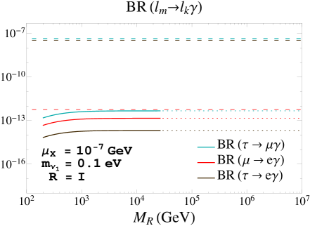
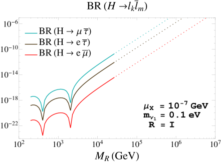
Figure 2: Predictions for the LFV decay rates as functions of MRsubscript𝑀𝑅M_{R} in the degenerate heavy neutrinos case. Left panel: BR(Hμτ¯)𝐻𝜇¯𝜏(H\to\mu\bar{\tau}) (upper blue line), BR(Heτ¯)𝐻𝑒¯𝜏(H\to e\bar{\tau}) (middle dark brown line), BR(Heμ¯)𝐻𝑒¯𝜇(H\to e\bar{\mu}) (lower red line). Right panel: BR(τμγ)𝜏𝜇𝛾(\tau\to\mu\gamma) (upper blue line), BR(μeγ)𝜇𝑒𝛾(\mu\to e\gamma) (middle red line), BR(τeγ)𝜏𝑒𝛾(\tau\to e\gamma) (lower dark brown line). The other input parameters are set to μX=107GeVsubscript𝜇𝑋superscript107GeV\mu_{X}=10^{-7}\,{\rm GeV}, mν1=0.1eVsubscript𝑚subscript𝜈10.1eVm_{\nu_{1}}=0.1\,{\rm eV}, R=I𝑅𝐼R=I. The dotted lines in both panels indicate nonperturbative neutrino Yukawa couplings. The horizontal dashed lines in the right panel are the present (90%percent9090\% C.L.) upper bounds on the radiative decays: BR(τμγ)<4.4×10⁸𝜏𝜇𝛾4.4superscript108(\tau\to\mu\gamma)<4.4\times 10^{-8} [53] (blue line), BR(τeγ)<3.3×10⁸𝜏𝑒𝛾3.3superscript108(\tau\to e\gamma)<3.3\times 10^{-8} [53] (dark brown line), BR(μeγ)<5.7×10¹³𝜇𝑒𝛾5.7superscript1013(\mu\to e\gamma)<5.7\times 10^{-13} [29] (red line).

The case of (nearly) degenerate heavy neutrinos is implemented here by choosing degenerate entries in MR=diag(MR1,MR2,MR3)subscript𝑀𝑅diagsubscript𝑀subscript𝑅1subscript𝑀subscript𝑅2subscript𝑀subscript𝑅3M_{R}={\rm diag}(M_{R_{1}},M_{R_{2}},M_{R_{3}}) and in μX=diag(μX1,μX2,μX3)subscript𝜇𝑋diagsubscript𝜇subscript𝑋1subscript𝜇subscript𝑋2subscript𝜇subscript𝑋3\mu_{X}={\rm diag}(\mu_{X_{1}},\mu_{X_{2}},\mu_{X_{3}}), i.e., by setting MRi=MRsubscript𝑀subscript𝑅𝑖subscript𝑀𝑅M_{R_{i}}=M_{R} and μXi=μXsubscript𝜇subscript𝑋𝑖subscript𝜇𝑋\mu_{X_{i}}=\mu_{X} (i=1,2,3𝑖123i=1,2,3).

First we show in fig. 2 the results for all the LFV rates as functions of the common right-handed neutrino mass parameter MRsubscript𝑀𝑅M_{R} for all the LFV Higgs decay channels (left panel) and for all the LFV radiative decay channels (right panel). Here we have fixed the other input parameters to μX=107subscript𝜇𝑋superscript107\mu_{X}=10^{-7} GeV, mν1=0.1subscript𝑚subscript𝜈10.1m_{\nu_{1}}=0.1 eV, and R=I𝑅𝐼R=I. As expected, we find that the largest LFV Higgs decay rates are for BR(Hμτ¯𝐻𝜇¯𝜏H\to\mu\bar{\tau}) and the largest radiative decay rates are for BR(τμγ𝜏𝜇𝛾\tau\to\mu\gamma). We also see that, for this particular choice of input parameters, all the predictions for the LFV Higgs decays are allowed by the present experimental upper bounds on the three radiative decays (dashed horizontal lines in all our plots for the radiative decays) for all explored values of MRsubscript𝑀𝑅M_{R} in the interval (200,107)GeV200superscript107GeV(200,10^{7})\,{\rm GeV}. Besides, it shows clearly that the most constraining radiative decay at present is by far the μeγ𝜇𝑒𝛾\mu\to e\gamma radiative decay. This is so in all the cases explored in this work, so whenever we wish to conclude on the allowed LFVHD rates we will focus mainly on this radiative channel.

Regarding the MRsubscript𝑀𝑅M_{R} dependence shown in fig. 2, we clearly see that the LFVHD rates grow faster with MRsubscript𝑀𝑅M_{R} than the radiative decays which indeed tend to a constant value for MRsubscript𝑀𝑅M_{R} above 103similar-toabsentsuperscript103\sim 10^{3} GeV. In fact, the LFVHD rates can reach quite sizable values at the large MRsubscript𝑀𝑅M_{R} region of these plots, yet are allowed by the constraints on the radiative decays. For instance, we obtain BR(Hμτ¯)106similar-to𝐻𝜇¯𝜏superscript106(H\to\mu\bar{\tau})\sim 10^{-6} for MR=4×10⁵subscript𝑀𝑅4superscript105M_{R}=4\times 10^{5} GeV. However, our requirement of perturbativity for the neutrino Yukawa coupling entries, see eq. (16), does not allow for such large MRsubscript𝑀𝑅M_{R} values leading to too-large Yνsubscript𝑌𝜈Y_{\nu} values in the framework of our parametrization of eq. (11). Indeed, the exclusion region for MRsubscript𝑀𝑅M_{R} from perturbativity of Yνsubscript𝑌𝜈Y_{\nu} (given by the dotted lines in these plots), forbids these large MRsubscript𝑀𝑅M_{R} values. For the specific input parameter values of this fig. 2, the forbidden values are for MRsubscript𝑀𝑅M_{R} above 3×1043superscript1043\times 10^{4} GeV, and this leads to maximum allowed values of BR(Hμτ¯)2×10¹¹similar-to𝐻𝜇¯𝜏2superscript1011(H\to\mu\bar{\tau})\sim 2\times 10^{-11}, BR(Heτ¯)1012similar-to𝐻𝑒¯𝜏superscript1012(H\to e\bar{\tau})\sim 10^{-12}, and BR(Heμ¯)5×10¹⁵similar-to𝐻𝑒¯𝜇5superscript1015(H\to e\bar{\mu})\sim 5\times 10^{-15}.

Refer to caption Refer to caption
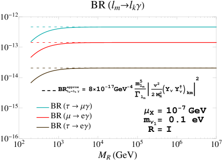
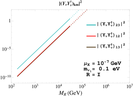
Figure 3: Comparison of the full one-loop and approximate rates for the radiative decays lmlkγsubscript𝑙𝑚subscript𝑙𝑘𝛾l_{m}\to l_{k}\gamma and their relation with the (YνYν)kmsubscriptsubscript𝑌𝜈superscriptsubscript𝑌𝜈𝑘𝑚(Y_{\nu}Y_{\nu}^{\dagger})_{km} nondiagonal matrix elements in the degenerate heavy neutrinos case. Left panel: full one-loop rates (solid lines) and approximate rates (dashed lines) as functions of MRsubscript𝑀𝑅M_{R}. Right panel: |(YνYν)km|2superscriptsubscriptsubscript𝑌𝜈superscriptsubscript𝑌𝜈𝑘𝑚2|(Y_{\nu}Y_{\nu}^{\dagger})_{km}|^{2} versus MRsubscript𝑀𝑅M_{R} for km=23𝑘𝑚23km=23 (blue line), km=12𝑘𝑚12km=12 (red line), and km=13𝑘𝑚13km=13 (dark brown line). Dotted lines indicate nonperturbative neutrino Yukawa couplings. The other input parameters are set to μX=107GeVsubscript𝜇𝑋superscript107GeV\mu_{X}=10^{-7}\,{\rm GeV}, mν1=0.1eVsubscript𝑚subscript𝜈10.1eVm_{\nu_{1}}=0.1\,{\rm eV}, and R=I𝑅𝐼R=I.

The qualitatively different functional behavior with MRsubscript𝑀𝑅M_{R} of the LFVHD and the radiative rates shown by fig. 2 is an interesting feature that we wish to explore further. Whereas the BR(lmlkγ)subscript𝑙𝑚subscript𝑙𝑘𝛾(l_{m}\to~{}l_{k}\gamma) rates follow the expected behavior with MRsubscript𝑀𝑅M_{R} as derived from their dependence with the relevant (YνYν)kmsubscriptsubscript𝑌𝜈superscriptsubscript𝑌𝜈𝑘𝑚(Y_{\nu}Y_{\nu}^{\dagger})_{km} element, the BR(Hlkl¯m𝐻subscript𝑙𝑘subscript¯𝑙𝑚H\to l_{k}\bar{l}_{m}) rates do not follow this same pattern. As it is clearly illustrated in fig. 3, the radiative decay rates can be well approximated for large MRsubscript𝑀𝑅M_{R} by a simple function of |(YνYν)km|2superscriptsubscriptsubscript𝑌𝜈superscriptsubscript𝑌𝜈𝑘𝑚2|(Y_{\nu}Y_{\nu}^{\dagger})_{km}|^{2} given by

BRlmlkγapprox=8×10¹⁷mlm5(GeV5)Γlm(GeV)|v22MR2(YνYν)km|2,subscriptsuperscriptBRapproxsubscript𝑙𝑚subscript𝑙𝑘𝛾8superscript1017superscriptsubscript𝑚subscript𝑙𝑚5superscriptGeV5subscriptΓsubscript𝑙𝑚GeVsuperscriptsuperscript𝑣22superscriptsubscript𝑀𝑅2subscriptsubscript𝑌𝜈superscriptsubscript𝑌𝜈𝑘𝑚2{\rm BR}^{\rm approx}_{l_{m}\to l_{k}\gamma}=8\times 10^{-17}\frac{m_{l_{m}}^{5}({\rm GeV}^{5})}{\Gamma_{l_{m}}{\rm(GeV)}}\bigg{|}\frac{v^{2}}{2M_{R}^{2}}(Y_{\nu}Y_{\nu}^{\dagger})_{km}\bigg{|}^{2}, (28)

which provides predictions very close to the exact rates (given by the solid lines) for MR>103subscript𝑀𝑅superscript103M_{R}>10^{3} GeV. Then we can understand the final constant behavior of all the radiative decay rates with MRsubscript𝑀𝑅M_{R}, since the |(YνYν)km|2superscriptsubscriptsubscript𝑌𝜈superscriptsubscript𝑌𝜈𝑘𝑚2|(Y_{\nu}Y_{\nu}^{\dagger})_{km}|^{2} elements grow with MRsubscript𝑀𝑅M_{R} approximately as MR4superscriptsubscript𝑀𝑅4M_{R}^{4} in the parametrization here used of eq. (11), as can be seen in the plot on the right in fig. 3. This simple behavior with MRsubscript𝑀𝑅M_{R} is certainly not the case of the LFVHD rates, and we conclude that these do not follow this same behavior with |(YνYν)km|2superscriptsubscriptsubscript𝑌𝜈superscriptsubscript𝑌𝜈𝑘𝑚2|(Y_{\nu}Y_{\nu}^{\dagger})_{km}|^{2}. This different functional behavior of BR(Hlkl¯m)𝐻subscript𝑙𝑘subscript¯𝑙𝑚(H\to l_{k}\bar{l}_{m}) with MRsubscript𝑀𝑅M_{R} will be further explored and clarified later.
Refer to caption Refer to caption
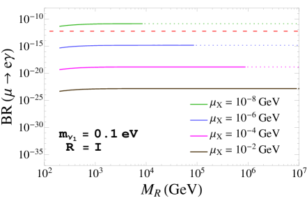
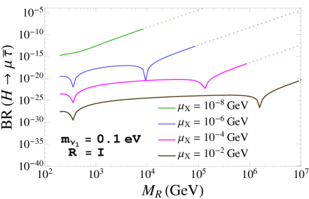
Figure 4: Branching ratios of Hμτ¯𝐻𝜇¯𝜏H\to\mu\overline{\tau} (left panel) and μeγ𝜇𝑒𝛾\mu\to e\gamma (right panel) as functions of MRsubscript𝑀𝑅M_{R} for different values of μX=(108,106,104,102)subscript𝜇𝑋superscript108superscript106superscript104superscript102\mu_{X}=(10^{-8},10^{-6},10^{-4},10^{-2}) GeV from top to bottom. In both panels, mν1=0.1subscript𝑚subscript𝜈10.1m_{\nu_{1}}=0.1 eV and R=I𝑅𝐼R=I. The horizontal red dashed line denotes the current experimental upper bound for μeγ𝜇𝑒𝛾\mu\to e\gamma, BR(μeγ𝜇𝑒𝛾\mu\to e\gamma) <5.7×10¹³absent5.7superscript1013<5.7\times 10^{-13} [29]. Dotted lines represent nonperturbative neutrino Yukawa couplings.

Next we study the sensitivity in the LFV rates to other choices of μXsubscript𝜇𝑋\mu_{X}. For this study we focus on the largest LFVHD rates, BR(Hμτ¯𝐻𝜇¯𝜏H\to\mu\bar{\tau}), and on the most constraining BR(μeγ)𝜇𝑒𝛾(\mu\to e\gamma) rates. In fig. 4 we show the predictions for the LFV rates for different values of μX=(108,106,104,102)subscript𝜇𝑋superscript108superscript106superscript104superscript102\mu_{X}=(10^{-8},10^{-6},10^{-4},10^{-2}) GeV. The other input parameters have been fixed here to mν1=0.1subscript𝑚subscript𝜈10.1m_{\nu_{1}}=0.1 eV and R=I𝑅𝐼R=I. On the left panel of fig. 4 we see again the increase of BR(Hμτ¯𝐻𝜇¯𝜏H\to\mu\overline{\tau}) as MRsubscript𝑀𝑅M_{R} grows, which is more pronounced in the region where MRsubscript𝑀𝑅M_{R} is large and μXsubscript𝜇𝑋\mu_{X} is low, and, therefore, where the Yukawa couplings are large [see eq. (11)]. We have checked that, in that region, the dominant diagrams are by far the divergent diagrams (1), (8), and (10), and that the BR(Hμτ¯𝐻𝜇¯𝜏H\to\mu\overline{\tau}) rates grow as MR4superscriptsubscript𝑀𝑅4M_{R}^{4}. In this plot, as well as in the previous plot of BR(Hlkl¯m𝐻subscript𝑙𝑘subscript¯𝑙𝑚H\to l_{k}\bar{l}_{m}) in fig. 2, we can also identify the appearance of different dips, which we have understood as destructive interferences among the various contributing diagrams. More precisely, we have checked that the dips that appear at large MRsubscript𝑀𝑅M_{R} and just before the MR4superscriptsubscript𝑀𝑅4M_{R}^{4} growing region are due to partial cancellations between diagrams (1),(8), and (10), while the other dips that appear at lower MRsubscript𝑀𝑅M_{R} happen among diagrams (2)-(6) [(7) and (9) are subleading]. These last diagrams have relevant contributions to BR(Hμτ¯𝐻𝜇¯𝜏H\to\mu\overline{\tau}) only for low values of the Yukawa couplings. We also observe a fast growth of the LFV Higgs rates as μXsubscript𝜇𝑋\mu_{X} decreases from 102superscript10210^{-2} GeV to 108superscript10810^{-8} GeV. However, not all the values of MRsubscript𝑀𝑅M_{R} and μXsubscript𝜇𝑋\mu_{X} are allowed, because they may generate nonperturbative Yuwaka entries, expressed again in this figure by dotted lines. Therefore, the largest LFV Higgs rates permitted by our perturbativity requirements [eq. (16)] are approximately BR(Hμτ¯𝐻𝜇¯𝜏H\to\mu\overline{\tau}) 109similar-toabsentsuperscript109\sim 10^{-9}, obtained for μX=108subscript𝜇𝑋superscript108\mu_{X}=10^{-8} GeV and MR104similar-to-or-equalssubscript𝑀𝑅superscript104M_{R}\simeq 10^{4} GeV. Larger values of MRsubscript𝑀𝑅M_{R}, for this choice of μXsubscript𝜇𝑋\mu_{X}, would produce Yukawa couplings that are not perturbative.

Nevertheless, we must pay attention to the predictions of BR(μeγ𝜇𝑒𝛾\mu\to e\gamma) for this choice of parameters, because they can be excluded by its quite restrictive present experimental upper bound, as shown on the right panel of fig. 4. In this plot, the dependence of BR(μeγ𝜇𝑒𝛾\mu\to e\gamma) on MRsubscript𝑀𝑅M_{R} is depicted, for the same choices of μXsubscript𝜇𝑋\mu_{X}, mν1subscript𝑚subscript𝜈1m_{\nu_{1}}, and R𝑅R as in the left panel. The horizontal red dashed line denotes again its current upper bound; see eq. (23). In addition to what we have already learned about the approximate behavior of the BR(μeγ𝜇𝑒𝛾\mu\to e\gamma) rates going as |(YνYν)12/MR2|2superscriptsubscriptsubscript𝑌𝜈superscriptsubscript𝑌𝜈12superscriptsubscript𝑀𝑅22|(Y_{\nu}Y_{\nu}^{\dagger})_{12}/M_{R}^{2}|^{2}, which explains the constant behavior with MRsubscript𝑀𝑅M_{R}, we also learn from this figure about the generic behavior with μXsubscript𝜇𝑋\mu_{X}, which leads to increasing LFV rates for decreasing μXsubscript𝜇𝑋\mu_{X} values, for both LFVHD and radiative processes. In particular, we see that small values of μX𝒪(108GeV)subscript𝜇𝑋𝒪superscript108GeV\mu_{X}\leq\mathcal{O}(10^{-8}~{}\rm{GeV}) lead to BR(μeγ𝜇𝑒𝛾\mu\to e\gamma) rates that are excluded by the present experimental upper bound. Taking this into account, the largest value of BR(Hμτ¯𝐻𝜇¯𝜏H\to\mu\overline{\tau}), for the choice of parameters fixed in fig. 4, that is allowed by the BR(μeγ𝜇𝑒𝛾\mu\to e\gamma) upper bound (this being more restrictive than the perturbativity requirement in this case) is 1012similar-toabsentsuperscript1012\sim 10^{-12}, which is obtained for MR=105subscript𝑀𝑅superscript105M_{R}=10^{5} GeV and μX=106subscript𝜇𝑋superscript106\mu_{X}=10^{-6} GeV.

Refer to caption Refer to caption
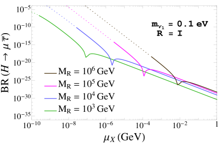
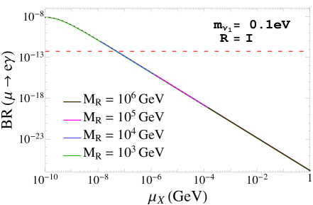
Figure 5: Branching ratios of Hμτ¯𝐻𝜇¯𝜏H\to\mu\overline{\tau} (left panel) and μeγ𝜇𝑒𝛾\mu\to e\gamma (right panel) as functions of μXsubscript𝜇𝑋\mu_{X} for different values of MR=(106,105,104,103)subscript𝑀𝑅superscript106superscript105superscript104superscript103M_{R}=(10^{6},10^{5},10^{4},10^{3}) GeV from top to bottom. In both panels, mν1=0.1subscript𝑚subscript𝜈10.1m_{\nu_{1}}=0.1 eV and R=I𝑅𝐼R=I. The horizontal red dashed line denotes the current experimental upper bound for μeγ𝜇𝑒𝛾\mu\to e\gamma, BR(μeγ𝜇𝑒𝛾\mu\to e\gamma) <5.7×10¹³absent5.7superscript1013<5.7\times 10^{-13} [29]. Dotted lines represent nonperturbative neutrino Yukawa couplings.

The behavior of BR(Hμτ¯𝐻𝜇¯𝜏H\to\mu\overline{\tau}) and BR(μeγ𝜇𝑒𝛾\mu\to e\gamma) as functions of μXsubscript𝜇𝑋\mu_{X}, for several values of MRsubscript𝑀𝑅M_{R}, mν1=0.1subscript𝑚subscript𝜈10.1m_{\nu_{1}}=0.1 eV, and R=I𝑅𝐼R=I, is displayed in fig. 5. As already seen in fig. 4, both LFV rates decrease as μXsubscript𝜇𝑋\mu_{X} grows; however, the functional dependence is not the same. The LFV radiative decay rates decrease as μX2superscriptsubscript𝜇𝑋2\mu_{X}^{-2}, in agreement with the approximate expression (28), while the LFVHD rates go as μX4superscriptsubscript𝜇𝑋4\mu_{X}^{-4} when the Yukawa couplings are large. For a fixed value of μXsubscript𝜇𝑋\mu_{X}, the larger MRsubscript𝑀𝑅M_{R} is, the larger BR(Hμτ¯𝐻𝜇¯𝜏H\to\mu\overline{\tau}) can be, while the prediction for BR(μeγ𝜇𝑒𝛾\mu\to e\gamma) is the same for any value of MRsubscript𝑀𝑅M_{R}. We have already learned this independence of the LFV radiative decays on MRsubscript𝑀𝑅M_{R} from the previous figure, which can be easily confirmed on the right panel of fig. 5, where all the lines for different values of MRsubscript𝑀𝑅M_{R} are superimposed. We observe again the existence of dips in the left panel of fig. 5. We also see in this figure that the smallest value of μXsubscript𝜇𝑋\mu_{X} allowed by the BR(μeγ𝜇𝑒𝛾\mu\to e\gamma) upper bound is μX5×108similar-tosubscript𝜇𝑋5superscript108\mu_{X}\sim 5\times 10^{-8} GeV, which is directly translated to a maximum allowed value of BR(Hμτ¯𝐻𝜇¯𝜏H\to\mu\overline{\tau}) 1011similar-toabsentsuperscript1011\sim 10^{-11}, for MR=104subscript𝑀𝑅superscript104M_{R}=10^{4} GeV.

Refer to caption Refer to caption
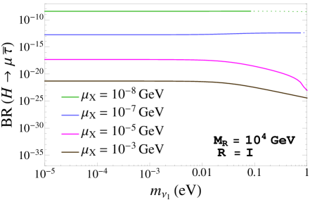
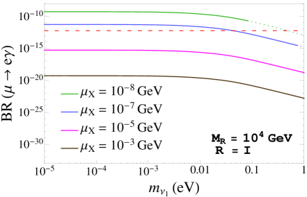
Figure 6: Branching ratios of Hμτ¯𝐻𝜇¯𝜏H\to\mu\overline{\tau} (left panel) and μeγ𝜇𝑒𝛾\mu\to e\gamma (right panel) as functions of mν1subscript𝑚subscript𝜈1m_{\nu_{1}} for different values of μX=(108,107,105,103)subscript𝜇𝑋superscript108superscript107superscript105superscript103\mu_{X}=(10^{-8},10^{-7},10^{-5},10^{-3}) GeV from top to bottom. In both panels, MR=104subscript𝑀𝑅superscript104M_{R}=10^{4} GeV and R=I𝑅𝐼R=I. The horizontal red dashed line denotes the current experimental upper bound for μeγ𝜇𝑒𝛾\mu\to e\gamma, BR(μeγ𝜇𝑒𝛾\mu\to e\gamma) <5.7×10¹³absent5.7superscript1013<5.7\times 10^{-13} [29]. Dotted lines represent nonperturbative neutrino Yukawa couplings [see eq. (16)].

The dependence of BR(Hμτ¯𝐻𝜇¯𝜏H\to\mu\overline{\tau}) and BR(μeγ𝜇𝑒𝛾\mu\to e\gamma) on the lightest neutrino mass mν1subscript𝑚subscript𝜈1m_{\nu_{1}} is studied in fig. 6, for several values of μXsubscript𝜇𝑋\mu_{X} with MR=104subscript𝑀𝑅superscript104M_{R}=10^{4} GeV and R=I𝑅𝐼R=I. For the chosen parameters in this figure, a similar dependence on mν1subscript𝑚subscript𝜈1m_{\nu_{1}} is observed in both observables, in which there is a flat behavior with mν1subscript𝑚subscript𝜈1m_{\nu_{1}} except for values of mν1greater-than-or-equivalent-tosubscript𝑚subscript𝜈1absentm_{\nu_{1}}\gtrsim 0.01 eV. For these values, the LFV rates decrease as mν1subscript𝑚subscript𝜈1m_{\nu_{1}} grows.

The behavior of BR(lmlkγsubscript𝑙𝑚subscript𝑙𝑘𝛾l_{m}\to l_{k}\gamma) with mν1subscript𝑚subscript𝜈1m_{\nu_{1}} can be understood from the fact that the flavor violation arises from the nondiagonal terms of (YνYν)kmsubscriptsubscript𝑌𝜈superscriptsubscript𝑌𝜈𝑘𝑚(Y_{\nu}Y_{\nu}^{\dagger})_{km}. In the simplified case of real R𝑅R and UPMNSsubscript𝑈PMNSU_{\rm PMNS} matrices, for diagonal and degenerate MRsubscript𝑀𝑅M_{R} and μXsubscript𝜇𝑋\mu_{X}, and by using eqs. (9) and (11), we find the following simple expression for the nondiagonal km𝑘𝑚km elements:

v2(YνYν)kmMR2{1μX(UPMNSΔm2UPMNST)km,formν12|Δmij2|,1μX(UPMNSΔm2UPMNST)km2mν1,formν12|Δmij2|,\frac{v^{2}\Big{(}Y_{\nu}Y_{\nu}^{\dagger}\Big{)}_{km}}{M_{R}^{2}}\approx\left\{\begin{array}[]{ll}\displaystyle{\frac{1}{\mu_{X}}\Big{(}U_{\rm PMNS}\sqrt{\Delta m^{2}}~{}U_{\rm PMNS}^{T}\Big{)}_{km}}&,\,{\rm for}~{}m_{\nu_{1}}^{2}\ll|\Delta m^{2}_{ij}|\,,\\ \\ \displaystyle{\frac{1}{\mu_{X}}\frac{\Big{(}U_{\rm PMNS}\Delta m^{2}~{}U_{\rm PMNS}^{T}\Big{)}_{km}}{2m_{\nu_{1}}}}&,\,{\rm for}~{}m_{\nu_{1}}^{2}\gg|\Delta m^{2}_{ij}|\,,\end{array}\right. (29)

where we have defined

Δm2diag(0,Δm212,Δm312),Δsuperscript𝑚2diag0Δsuperscriptsubscriptm212Δsuperscriptsubscriptm312\Delta m^{2}\equiv\rm{diag}(0,\Delta m_{21}^{2},\Delta m_{31}^{2})~{}, (30)

and we have expanded properly mν2subscript𝑚subscript𝜈2m_{\nu_{2}} and mν3subscript𝑚subscript𝜈3m_{\nu_{3}} in eq. (13) in terms of mν1subscript𝑚subscript𝜈1m_{\nu_{1}} and Δmij2Δsuperscriptsubscript𝑚𝑖𝑗2\Delta m_{ij}^{2}. Therefore, using eqs. (28)-(30), we conclude that the BR(μeγ𝜇𝑒𝛾\mu\to~{}e\gamma) rates have a flat behavior with mν1subscript𝑚subscript𝜈1m_{\nu_{1}} for low values of mν10.01eVless-than-or-similar-tosubscript𝑚subscript𝜈10.01eVm_{\nu_{1}}\lesssim 0.01~{}\rm{eV}, but they decrease with mν1subscript𝑚subscript𝜈1m_{\nu_{1}} for larger values, explaining the observed behavior in fig. 6.

By taking into account all the behaviors learned above, we have tried to find an approximate simple formula that could explain the main features of the BR(Hμτ¯𝐻𝜇¯𝜏H\to\mu\overline{\tau}) rates. As we have already said, in contrast to what we have seen for the LFV radiative decays in eq. (28), a simple functional dependence being proportional to |(YνYν)23|2superscriptsubscriptsubscript𝑌𝜈superscriptsubscript𝑌𝜈232|(Y_{\nu}Y_{\nu}^{\dagger})_{23}|^{2} is not enough to describe our results for the BR(Hμτ¯𝐻𝜇¯𝜏H\to\mu\overline{\tau}) rates. Considering that, in the region where the Yukawa couplings are large, the LFVHD rates are dominated by diagrams (1), (8), and (10), we have looked for a simple expression that could properly fit the contributions from these dominant diagrams. From this fit we have found the following approximate formula:

BRHμτ¯approx=107v4MR4|(YνYν)235.7(YνYνYνYν)23|2,subscriptsuperscriptBRapprox𝐻𝜇¯𝜏superscript107superscript𝑣4superscriptsubscript𝑀𝑅4superscriptsubscriptsubscript𝑌𝜈superscriptsubscript𝑌𝜈235.7subscriptsubscript𝑌𝜈superscriptsubscript𝑌𝜈subscript𝑌𝜈superscriptsubscript𝑌𝜈232{\rm BR}^{\rm approx}_{H\to\mu\bar{\tau}}=10^{-7}\frac{v^{4}}{M_{R}^{4}}~{}\Big{|}(Y_{\nu}Y_{\nu}^{\dagger})_{23}-5.7(Y_{\nu}Y_{\nu}^{\dagger}Y_{\nu}Y_{\nu}^{\dagger})_{23}\Big{|}^{2}, (31)

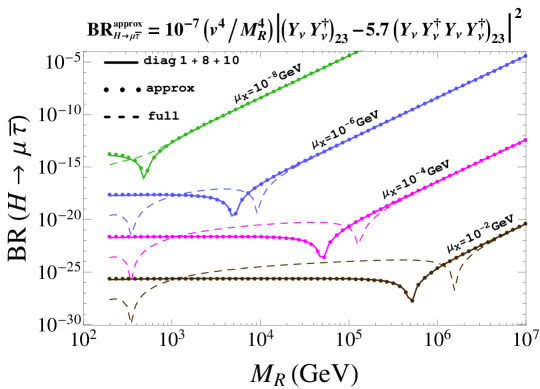
which turns out to work reasonably well. In fig. 7 we show the predicted rates of BR(Hμτ¯𝐻𝜇¯𝜏H\to\mu\overline{\tau}) with (1) the full one-loop formulas (dashed lines); (2) taking just the contributions from diagrams (1), (8), and (10) of fig. 1 (solid lines); and (3) using eq. (31) (dotted lines). We see clearly that this eq. (31) reproduces extremely well the contributions from diagrams (1), (8), and (10) and approximates reasonably well the full rates. The approximation is pretty good indeed for the MRsubscript𝑀𝑅M_{R} region above the dips. The change of functional behavior with MRsubscript𝑀𝑅M_{R} in the two different MRsubscript𝑀𝑅M_{R} regions, from nearly flat with MRsubscript𝑀𝑅M_{R} in the approximate result to fast growing as MR4similar-toabsentsuperscriptsubscript𝑀𝑅4\sim M_{R}^{4}, also gives a reasonable approach to the full result, as well as the appearance of dips. The location of the dips is however not so accurately described by the approximate formula, since in the region where the cancellation among the diagrams (1), (8), and (10) takes place the other diagrams (not considered in the fit) also contribute. Overall, we find the approximate formula given by eq. (31) very useful for generic estimates in the ISS, which could also be applied to other parametrizations of the neutrino Yukawa couplings.
Refer to caption
Figure 7: Comparison between the predicted rates for BR(Hμτ¯𝐻𝜇¯𝜏H\to\mu\overline{\tau}) taking (1) the full one-loop formulas (dashed lines); (2) just the contributions from diagrams (1), (8), and (10) of fig. 1 (solid lines); and (3) the approximate formula of eq. (31) (dotted lines)

This particular choice for the fitting function can be easily understood using the electroweak interaction basis of eq. (1) and applying the mass insertion approximation (MIA). Looking at the finite contribution coming from diagrams (1), (8), and (10), we can see that, at the lowest order in the MIA, the Higgs decay amplitude has a similar behavior to the dimension-six operator that governs the LFV radiative decays, which is proportional to

v2(YνYν)kmMR2.superscript𝑣2subscriptsubscript𝑌𝜈superscriptsubscript𝑌𝜈𝑘𝑚superscriptsubscript𝑀𝑅2\frac{v^{2}(Y_{\nu}Y_{\nu}^{\dagger})_{km}}{M_{R}^{2}}\,. (32)

However, there are other contributions to the Higgs decays that are not present in the case of the radiative decays, owing to the different chiral structure of the lepton flavor violating operators. For example, having two mass insertions of LR𝐿𝑅LR type, one in each internal neutrino line of a loop like that of diagram 1, will give a contribution to the amplitude proportional to

v2(YνYνYνYν)kmMR2.superscript𝑣2subscriptsubscript𝑌𝜈superscriptsubscript𝑌𝜈subscript𝑌𝜈superscriptsubscript𝑌𝜈𝑘𝑚superscriptsubscript𝑀𝑅2\frac{v^{2}(Y_{\nu}Y_{\nu}^{\dagger}Y_{\nu}Y_{\nu}^{\dagger})_{km}}{M_{R}^{2}}\,. (33)

Then, using again eqs. (11) and (9), we find the following simple expression:

v2(YνYνYνYν)kmMR2=MR2v2μX2(UPMNSΔm2UPMNST)km.superscript𝑣2subscriptsubscript𝑌𝜈superscriptsubscript𝑌𝜈subscript𝑌𝜈superscriptsubscript𝑌𝜈𝑘𝑚superscriptsubscript𝑀𝑅2superscriptsubscript𝑀𝑅2superscript𝑣2superscriptsubscript𝜇𝑋2subscriptsubscript𝑈PMNSΔsuperscript𝑚2superscriptsubscript𝑈PMNS𝑇𝑘𝑚\frac{v^{2}(Y_{\nu}Y_{\nu}^{\dagger}Y_{\nu}Y_{\nu}^{\dagger})_{km}}{M_{R}^{2}}=\frac{M_{R}^{2}}{v^{2}\mu_{X}^{2}}\Big{(}U_{\rm PMNS}\Delta m^{2}~{}U_{\rm PMNS}^{T}\Big{)}_{km}\,. (34)

Thus, we can clearly see from the above result that the second contribution in eq. (31) is the one that dominates at large MRsubscript𝑀𝑅M_{R} and low μXsubscript𝜇𝑋\mu_{X}, i.e., at large Yukawa couplings, and, indeed, it reproduces properly the behavior of BR(Hμτ¯𝐻𝜇¯𝜏H\to\mu\overline{\tau}) in this limit, with BR MR4/μX4proportional-toabsentsuperscriptsubscript𝑀𝑅4superscriptsubscript𝜇𝑋4\propto M_{R}^{4}/\mu_{X}^{4}. It is also independent of mν1subscript𝑚subscript𝜈1m_{\nu_{1}}, explaining the flat behavior in fig. 6 for low values of μXsubscript𝜇𝑋\mu_{X}. Moreover, if the two contributions in eq. (31) have opposite signs, they will interfere destructively, leading to a dip in the decay rate when both contributions are of the same size. From eqs. (29) and (34), we can deduce that the position of the dip should verify MR2μXconstantsimilar-tosuperscriptsubscript𝑀𝑅2subscript𝜇𝑋constantM_{R}^{-2}\mu_{X}\sim\mathrm{constant}, which is the behavior observed at large MRsubscript𝑀𝑅M_{R} in figs. 4-5. The other dips, which appear for MR300GeVsimilar-to-or-equalssubscript𝑀𝑅300GeVM_{R}\simeq 300\,\mathrm{GeV} in fig. 4, come from a destructive interference between the other diagrams, as we have said.
Refer to caption Refer to caption
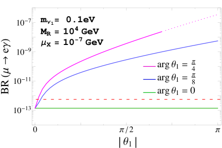
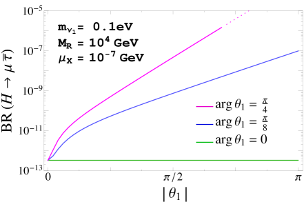
Figure 8: Branching ratios of Hμτ¯𝐻𝜇¯𝜏H\to\mu\overline{\tau} (left panel) and μeγ𝜇𝑒𝛾\mu\to e\gamma (right panel) as functions of |θ1|subscript𝜃1|\theta_{1}| for different values of argθ1subscript𝜃1\theta_{1}. In both panels, MR=104subscript𝑀𝑅superscript104M_{R}=10^{4} GeV, μX=107subscript𝜇𝑋superscript107\mu_{X}=10^{-7} GeV, and mν1=subscript𝑚subscript𝜈1absentm_{\nu_{1}}= 0.1 eV. The horizontal red dashed line denotes the current experimental upper bound for μeγ𝜇𝑒𝛾\mu\to e\gamma, BR(μeγ𝜇𝑒𝛾\mu\to e\gamma) <5.7×10¹³absent5.7superscript1013<5.7\times 10^{-13} [29]. Dotted lines represent nonperturbative neutrino Yukawa couplings [see eq. (16)].

Next, we display in fig. 8 the dependence of the Hμτ¯𝐻𝜇¯𝜏H\to\mu\overline{\tau} and μeγ𝜇𝑒𝛾\mu\to e\gamma decay rates on |θ1|subscript𝜃1|\theta_{1}| for different values of argθ1=0,π/8,π/4subscript𝜃10𝜋8𝜋4\theta_{1}=0,\pi/8,\pi/4, with MR=104subscript𝑀𝑅superscript104M_{R}=10^{4} GeV, μX=107subscript𝜇𝑋superscript107\mu_{X}=10^{-7} GeV, and mν1=subscript𝑚subscript𝜈1absentm_{\nu_{1}}= 0.1 eV. First of all, we highlight the flat behavior of both LFV rates with |θ1|subscript𝜃1|\theta_{1}| for real R𝑅R matrix (argθ1subscript𝜃1\theta_{1} = 0), which is a direct consequence of the degeneracy of MRsubscript𝑀𝑅M_{R} and μXsubscript𝜇𝑋\mu_{X}. In other words, the LFV rates for the degenerate heavy neutrinos case are independent of R𝑅R if it is real. Once we abandon the real case and consider values of argθ1subscript𝜃1\theta_{1} different from zero, a strong dependence on |θ1|subscript𝜃1|\theta_{1}| appears. The larger |θ1|subscript𝜃1|\theta_{1}| and/or argθ1subscript𝜃1\theta_{1} are, the larger the LFV rates become. On the other hand, only values of |θ1|subscript𝜃1|\theta_{1}| lower than π/32𝜋32\pi/32 with argθ1=π/8subscript𝜃1𝜋8\theta_{1}=\pi/8 in this figure are allowed by the μeγ𝜇𝑒𝛾\mu\to e\gamma constraint, which allows us to reach values of BR(Hμτ¯𝐻𝜇¯𝜏H\to\mu\bar{\tau}) 1012similar-toabsentsuperscript1012\sim 10^{-12} at the most. We have also explored the LFV rates as functions of complex θ2subscript𝜃2\theta_{2} and θ3subscript𝜃3\theta_{3} and we have reached similar conclusions as for θ1subscript𝜃1\theta_{1}. Therefore, by choosing complex θ1,2,3subscript𝜃123\theta_{1,2,3} the LFV Higgs decay rates that are allowed by the upper bounds on the radiative decays do not increase with respect to the real case, which is equal to the previous R=I𝑅𝐼R=I reference case, due to the independence on real R𝑅R, as we have already said.

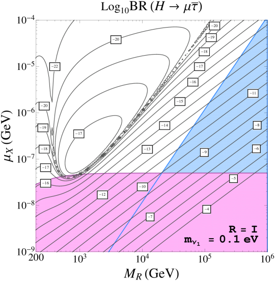
Once we have studied the behavior of all the LFV observables considered here with the most relevant parameters, we next present the results for the maximum allowed LFV Higgs decay rates in the case of heavy degenerate neutrinos. The plot in fig. 9 shows the contour lines of BR(Hμτ¯𝐻𝜇¯𝜏H\to\mu\bar{\tau}) in the (MR,μX)subscript𝑀𝑅subscript𝜇𝑋(M_{R},\mu_{X}) plane for R=I𝑅𝐼R=I and mν1=0.1eVsubscript𝑚subscript𝜈10.1eVm_{\nu_{1}}=0.1\,{\rm eV}. The horizontal area in pink is excluded by not respecting the present upper bound on BR(μeγ)𝜇𝑒𝛾(\mu\to e\gamma). The oblique area in blue is excluded by not respecting the perturbativity of the neutrino Yukawa couplings. These contour lines summarize the previously learned behavior with MRsubscript𝑀𝑅M_{R} and μXsubscript𝜇𝑋\mu_{X}, which lead to the largest values for the LFVHD rates in the bottom right-hand corner of the plot, i.e., at large MRsubscript𝑀𝑅M_{R} and small μXsubscript𝜇𝑋\mu_{X}. We also notice the appearance of dips in the (MR,μX)subscript𝑀𝑅subscript𝜇𝑋(M_{R},\mu_{X}) plane that correspond to the previously commented dips in the previous figures. The most important conclusion from this contour plot is that the maximum allowed LFVHD rate is approximately BR(Hμτ¯)1010similar-to𝐻𝜇¯𝜏superscript1010(H\to\mu\bar{\tau})\sim 10^{-10} and it is found for MR2×104GeVsimilar-tosubscript𝑀𝑅2superscript104GeVM_{R}\sim 2\times 10^{4}\,{\rm GeV} and μX5×108GeVsimilar-tosubscript𝜇𝑋5superscript108GeV\mu_{X}\sim 5\times 10^{-8}\,{\rm GeV}. We have found similar conclusions for BR(Heτ¯)𝐻𝑒¯𝜏(H\to e\bar{\tau}).

Refer to caption
Figure 9: Contour lines of BR(Hμτ¯𝐻𝜇¯𝜏H\to\mu\bar{\tau}) in the (MR,μX)subscript𝑀𝑅subscript𝜇𝑋(M_{R},\mu_{X}) plane for R=I𝑅𝐼R=I and mν1=0.1eVsubscript𝑚subscript𝜈10.1eVm_{\nu_{1}}=0.1\,{\rm eV}. The horizontal area in pink is excluded by the upper bound on BR(μeγ)𝜇𝑒𝛾(\mu\to e\gamma). The oblique area in blue is excluded by the perturbativity requirement of the neutrino Yukawa couplings.

4.2 Hierarchical heavy neutrinos

The case of hierarchical heavy neutrinos refers here to hierarchical masses among generations and it is implemented by choosing hierarchical entries in the MR=diag(MR1,MR2,MR3)subscript𝑀𝑅diagsubscript𝑀subscript𝑅1subscript𝑀subscript𝑅2subscript𝑀subscript𝑅3M_{R}={\rm diag}(M_{R_{1}},M_{R_{2}},M_{R_{3}}) matrix. As for the μX=diag(μX1,μX2,μX3)subscript𝜇𝑋diagsubscript𝜇subscript𝑋1subscript𝜇subscript𝑋2subscript𝜇subscript𝑋3\mu_{X}={\rm diag}(\mu_{X_{1}},\mu_{X_{2}},\mu_{X_{3}}) matrix that introduces the tiny splitting within the heavy masses in the same generation we choose it here to be degenerate, μX1,2,3=μXsubscript𝜇subscript𝑋123subscript𝜇𝑋\mu_{X_{1,2,3}}=\mu_{X}. We focus on the normal hierarchy MR1<MR2<MR3subscript𝑀subscript𝑅1subscript𝑀subscript𝑅2subscript𝑀subscript𝑅3M_{R_{1}}<M_{R_{2}}<M_{R_{3}}, since we have found similar conclusions for other hierarchies.

The results for the LFV rates in the MR1<MR2<MR3subscript𝑀subscript𝑅1subscript𝑀subscript𝑅2subscript𝑀subscript𝑅3M_{R_{1}}<M_{R_{2}}<M_{R_{3}} hierarchical case are shown in fig. 10.
Refer to caption Refer to caption
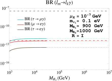
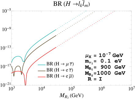
Figure 10: Predictions for the LFV decay rates as functions of MR3subscript𝑀subscript𝑅3M_{R_{3}} in the hierarchical heavy neutrinos case with MR1<MR2<MR3subscript𝑀subscript𝑅1subscript𝑀subscript𝑅2subscript𝑀subscript𝑅3M_{R_{1}}<M_{R_{2}}<M_{R_{3}}. Left panel: BR(Hμτ¯)𝐻𝜇¯𝜏(H\to\mu\bar{\tau}) (upper blue line), BR(Heτ¯)𝐻𝑒¯𝜏(H\to e\bar{\tau}) (middle dark brown line), BR(Heμ¯)𝐻𝑒¯𝜇(H\to e\bar{\mu}) (lower red line). Right panel: BR(τμγ)𝜏𝜇𝛾(\tau\to\mu\gamma) (upper blue line), BR(μeγ)𝜇𝑒𝛾(\mu\to e\gamma) (middle red line), BR(τeγ)𝜏𝑒𝛾(\tau\to e\gamma) (lower dark brown line). The other input parameters are set to μX=107GeVsubscript𝜇𝑋superscript107GeV\mu_{X}=10^{-7}\,{\rm GeV}, mν1=0.1eVsubscript𝑚subscript𝜈10.1eVm_{\nu_{1}}=0.1\,{\rm eV}, MR1=900GeVsubscript𝑀subscript𝑅1900GeVM_{R_{1}}=900\,{\rm GeV}, MR2=1000GeVsubscript𝑀subscript𝑅21000GeVM_{R_{2}}=1000\,{\rm GeV}, and R=I𝑅𝐼R=I. The dotted lines in both panels indicate nonperturbative neutrino Yukawa couplings. The horizontal dashed lines in the right panel are the present (90%percent9090\% C.L.) upper bounds on the radiative decays: BR(τμγ)<4.4×10⁸𝜏𝜇𝛾4.4superscript108(\tau\to\mu\gamma)<4.4\times 10^{-8} [53] (blue line), BR(τeγ)<3.3×10⁸𝜏𝑒𝛾3.3superscript108(\tau\to e\gamma)<3.3\times 10^{-8} [53] (dark brown line), and BR(μeγ)<5.7×10¹³𝜇𝑒𝛾5.7superscript1013(\mu\to e\gamma)<5.7\times 10^{-13} [29] (red line).

This figure shows that the behavior of the LFV rates in the hierarchical case with respect to the heaviest neutrino mass MR3subscript𝑀subscript𝑅3M_{R_{3}} is very similar to the one found previously for the degenerate case with respect to the common MRsubscript𝑀𝑅M_{R}. The BR(Hlkl¯m)𝐻subscript𝑙𝑘subscript¯𝑙𝑚(H\to l_{k}\bar{l}_{m}) rates grow fast with MR3subscript𝑀subscript𝑅3M_{R_{3}} at large MR3>3000GeVsubscript𝑀subscript𝑅33000GeVM_{R_{3}}>3000\,{\rm GeV}, whereas the BR(lmlkγ)subscript𝑙𝑚subscript𝑙𝑘𝛾(l_{m}\to l_{k}\gamma) rates stay flat with MR3subscript𝑀subscript𝑅3M_{R_{3}}. Again, there are dips in the BR(Hlkl¯m)𝐻subscript𝑙𝑘subscript¯𝑙𝑚(H\to l_{k}\bar{l}_{m}) rates due to the destructive interferences among the contributing diagrams. We also observe in this plot that, for the chosen parameters, the size that the BR(Hlkl¯m)𝐻subscript𝑙𝑘subscript¯𝑙𝑚(H\to l_{k}\bar{l}_{m}) rates can reach in this hierarchical scenario is larger than in the previous degenerate case. For instance, BR(Hμτ¯)𝐻𝜇¯𝜏(H\to\mu\bar{\tau}) reaches 109superscript10910^{-9} at MR3=3×10⁴GeVsubscript𝑀subscript𝑅33superscript104GeVM_{R_{3}}=3\times 10^{4}\,{\rm GeV}, to be compared with 1010superscript101010^{-10} at MR=3×10⁴GeVsubscript𝑀𝑅3superscript104GeVM_{R}=3\times 10^{4}\,{\rm GeV} that we got in fig. 2 for the degenerate case. We have found this same behavior of enhanced LFVHD rates by approximately one order of magnitude in the hierarchical case as compared to the degenerate case in most of the explored parameter space regions.

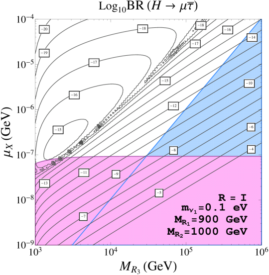
This same enhancement can also be seen in the contour plot in fig. 11 where the maximum allowed BR(Hμτ¯)𝐻𝜇¯𝜏(H\to\mu\bar{\tau}) rates reach values up to about 109superscript10910^{-9} for MR1=900GeVsubscript𝑀subscript𝑅1900GeVM_{R_{1}}=900\,{\rm GeV}, MR2=1000GeVsubscript𝑀subscript𝑅21000GeVM_{R_{2}}=1000\,{\rm GeV}, MR3=3×10⁴GeVsubscript𝑀subscript𝑅33superscript104GeVM_{R_{3}}=3\times 10^{4}\,{\rm GeV}, μX=107GeVsubscript𝜇𝑋superscript107GeV\mu_{X}=10^{-7}\,{\rm GeV}, and R=I𝑅𝐼R=I.

Refer to caption
Figure 11: Contour lines of BR(Hμτ¯𝐻𝜇¯𝜏H\to\mu\bar{\tau}) in the (MR3,μX)subscript𝑀subscript𝑅3subscript𝜇𝑋(M_{R_{3}},\mu_{X}) plane for R=I𝑅𝐼R=I, mν1=0.1eVsubscript𝑚subscript𝜈10.1eVm_{\nu_{1}}=0.1\,{\rm eV}, MR1=900GeVsubscript𝑀subscript𝑅1900GeVM_{R_{1}}=900\,{\rm GeV}, and MR2=1000GeVsubscript𝑀subscript𝑅21000GeVM_{R_{2}}=1000\,{\rm GeV}. The horizontal area in pink is disallowed by the upper bound on BR(μeγ)𝜇𝑒𝛾(\mu\to e\gamma). The oblique area in blue is disallowed by the perturbativity requirement of the neutrino Yukawa couplings.

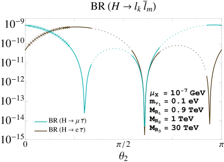
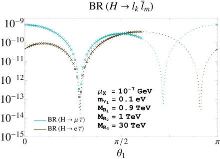
Finally, since in the hierarchical case, in contrast to the degenerate case, there is a dependence on the R𝑅R matrix even if it is real, we have also explored the behavior with the real θ1,2,3subscript𝜃123\theta_{1,2,3} angles. We have found that for this particular hierarchy, MR1<MR2<MR3subscript𝑀subscript𝑅1subscript𝑀subscript𝑅2subscript𝑀subscript𝑅3M_{R_{1}}<M_{R_{2}}<M_{R_{3}}, there is near independence with θ3subscript𝜃3\theta_{3} but there is a clear dependence with θ1subscript𝜃1\theta_{1} and θ2subscript𝜃2\theta_{2}, as it is illustrated in fig. 12. These plots show that the BR(Hlkl¯m)𝐻subscript𝑙𝑘subscript¯𝑙𝑚(H\to l_{k}\bar{l}_{m}) rates for θ1,20subscript𝜃120\theta_{1,2}\neq 0 can indeed increase or decrease with respect to the reference R=I𝑅𝐼R=I case. In particular, for 0<θ1<π0subscript𝜃1𝜋0<\theta_{1}<\pi we find that BR(Hμτ¯𝐻𝜇¯𝜏H\to\mu\bar{\tau}) is always lower than for R=I𝑅𝐼R=I, whereas BR(Heτ¯𝐻𝑒¯𝜏H\to e\bar{\tau}) can be one order of magnitude larger than for R=I𝑅𝐼R=I if θ1subscript𝜃1\theta_{1} is near π/2𝜋2\pi/2. For the case of 0<θ2<π0subscript𝜃2𝜋0<\theta_{2}<\pi, we find again that BR(Hμτ¯𝐻𝜇¯𝜏H\to\mu\bar{\tau}) is always lower than for R=I𝑅𝐼R=I, and BR(Heτ¯𝐻𝑒¯𝜏H\to e\bar{\tau}) can be one order of magnitude larger than for R=I𝑅𝐼R=I if θ2subscript𝜃2\theta_{2} is near π/4𝜋4\pi/4. In this latter case, it is interesting to notice that the region of θ2subscript𝜃2\theta_{2} close to π/4𝜋4\pi/4 where BR(Heτ¯𝐻𝑒¯𝜏H\to e\bar{\tau}) reaches the maximum value close to 109superscript10910^{-9} is allowed by all the constraints. The results for the other decay BR(Heμ¯𝐻𝑒¯𝜇H\to e\bar{\mu}) are not shown here because they again give much smaller rates, as in the degenerate case. We have also tried other choices for the hierarchies among the three heavy masses MR1,2,3subscript𝑀subscript𝑅123M_{R_{1,2,3}} and we have found similar conclusions.
Refer to caption Refer to caption
Figure 12: Predictions for BR(Hμτ¯𝐻𝜇¯𝜏H\to\mu\bar{\tau}) (blue lines) and BR(Heτ¯𝐻𝑒¯𝜏H\to e\bar{\tau}) (dark brown lines) rates as a function of real θ1subscript𝜃1\theta_{1} (left panel) and θ2subscript𝜃2\theta_{2} (right panel). The other input parameters are set to μX=107subscript𝜇𝑋superscript107\mu_{X}=10^{-7} GeV, mν1=0.1subscript𝑚subscript𝜈10.1m_{\nu_{1}}=0.1 eV, MR1=0.9subscript𝑀subscript𝑅10.9M_{R_{1}}=0.9 TeV, MR2=1subscript𝑀subscript𝑅21M_{R_{2}}=1 TeV, MR3=30subscript𝑀subscript𝑅330M_{R_{3}}=30 TeV, θ2=θ3=0subscript𝜃2subscript𝜃30\theta_{2}=\theta_{3}=0 in the left panel and θ1=θ3=0subscript𝜃1subscript𝜃30\theta_{1}=\theta_{3}=0 in the right panel. The dotted lines indicate nonperturbative neutrino Yukawa couplings and the crossed lines are excluded by the present upper bound on BR(μeγ𝜇𝑒𝛾\mu\to e\gamma). The solid lines are allowed by all the constraints.

4.3 ISS scenarios with large LFV Higgs decay rates

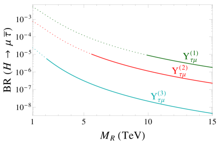
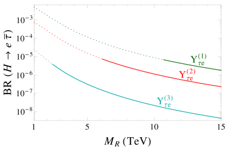
In this section we explore the implications on LFV Higgs decays of going beyond the simplest previous hypothesis of diagonal μXsubscript𝜇𝑋\mu_{X} and MRsubscript𝑀𝑅M_{R} mass matrices in the ISS model. In particular, given the interesting possibility of decoupling the low energy neutrino physics from the LFV physics in this ISS model, by the proper choice of the input parameters, we will look for specific ISS scenarios with nondiagonal μXsubscript𝜇𝑋\mu_{X} while keeping diagonal MRsubscript𝑀𝑅M_{R} that can provide the largest LFV Higgs decay rates and at the same time be compatible with the neutrino data and the present experimental upper bounds on the radiative decays. Here, we will focus on the case of degenerate MRsubscript𝑀𝑅M_{R} and will explore only the LFV Higgs decay channels with the largest rates, namely, Hμτ¯𝐻𝜇¯𝜏H\to\mu\bar{\tau} and Heτ¯𝐻𝑒¯𝜏H\to e\bar{\tau}.

In order to localize the class of scenarios leading to large and allowed LFVHD rates, we first make a rough estimate of the expected maximal rates for the Hμτ¯𝐻𝜇¯𝜏H\to\mu\bar{\tau} channel by using our approximate formula of eq. (31), which is given just in terms of the neutrino Yukawa coupling matrix Yνsubscript𝑌𝜈Y_{\nu} and MRsubscript𝑀𝑅M_{R}. On the other hand, in order to keep the predictions for the radiative decays below their corresponding experimental upper bounds, we need to require a maximum value for the nondiagonal (YνYν)ijsubscriptsubscript𝑌𝜈superscriptsubscript𝑌𝜈𝑖𝑗(Y_{\nu}Y_{\nu}^{\dagger})_{ij} entries. By using our approximate formula of eq. (28) and the present bounds in eqs. (23)-(25), we get

v2(YνYν)12max/MR2superscript𝑣2superscriptsubscriptsubscript𝑌𝜈superscriptsubscript𝑌𝜈12maxsuperscriptsubscript𝑀𝑅2\displaystyle v^{2}(Y_{\nu}Y_{\nu}^{\dagger})_{12}^{\rm max}/M_{R}^{2} similar-to\displaystyle\sim 2.5×105,2.5superscript105\displaystyle 2.5\times 10^{-5}, (35)
v2(YνYν)13max/MR2superscript𝑣2superscriptsubscriptsubscript𝑌𝜈superscriptsubscript𝑌𝜈13maxsuperscriptsubscript𝑀𝑅2\displaystyle v^{2}(Y_{\nu}Y_{\nu}^{\dagger})_{13}^{\rm max}/M_{R}^{2} similar-to\displaystyle\sim 0.015,0.015\displaystyle 0.015, (36)
v2(YνYν)23max/MR2superscript𝑣2superscriptsubscriptsubscript𝑌𝜈superscriptsubscript𝑌𝜈23maxsuperscriptsubscript𝑀𝑅2\displaystyle v^{2}(Y_{\nu}Y_{\nu}^{\dagger})_{23}^{\rm max}/M_{R}^{2} similar-to\displaystyle\sim 0.017.0.017\displaystyle 0.017. (37)

Then, in order to simplify our search, and given the above relative strong suppression of the 12 element, it seems reasonable to neglect it against the other off-diagonal elements. In that case, by assuming (YνYν)120similar-to-or-equalssubscriptsubscript𝑌𝜈superscriptsubscript𝑌𝜈120(Y_{\nu}Y_{\nu}^{\dagger})_{12}\simeq 0 we get

(YνYνYνYν)23(YνYν)22(YνYν)23+(YνYν)23(YνYν)33,similar-to-or-equalssubscriptsubscript𝑌𝜈superscriptsubscript𝑌𝜈subscript𝑌𝜈superscriptsubscript𝑌𝜈23subscriptsubscript𝑌𝜈superscriptsubscript𝑌𝜈22subscriptsubscript𝑌𝜈superscriptsubscript𝑌𝜈23subscriptsubscript𝑌𝜈superscriptsubscript𝑌𝜈23subscriptsubscript𝑌𝜈superscriptsubscript𝑌𝜈33(Y_{\nu}Y_{\nu}^{\dagger}Y_{\nu}Y_{\nu}^{\dagger})_{23}\simeq(Y_{\nu}Y_{\nu}^{\dagger})_{22}(Y_{\nu}Y_{\nu}^{\dagger})_{23}+(Y_{\nu}Y_{\nu}^{\dagger})_{23}(Y_{\nu}Y_{\nu}^{\dagger})_{33}, (38)

and the approximate formula of eq. (31) can then be rewritten as follows:

BRHμτ¯approx=107|v2MR2(YνYν)23|2|15.7((YνYν)22+(YνYν)33)|2.subscriptsuperscriptBRapprox𝐻𝜇¯𝜏superscript107superscriptsuperscript𝑣2superscriptsubscript𝑀𝑅2subscriptsubscript𝑌𝜈superscriptsubscript𝑌𝜈232superscript15.7subscriptsubscript𝑌𝜈superscriptsubscript𝑌𝜈22subscriptsubscript𝑌𝜈superscriptsubscript𝑌𝜈332{\rm BR}^{\rm approx}_{H\to\mu\bar{\tau}}=10^{-7}~{}\Big{|}\frac{v^{2}}{M_{R}^{2}}(Y_{\nu}Y_{\nu}^{\dagger})_{23}\Big{|}^{2}~{}\Big{|}1-5.7\Big{(}(Y_{\nu}Y_{\nu}^{\dagger})_{22}+(Y_{\nu}Y_{\nu}^{\dagger})_{33}\Big{)}\Big{|}^{2}. (39)

This equation clearly shows that the maximal BR(Hμτ¯𝐻𝜇¯𝜏H\to\mu\bar{\tau}) rates are obtained for the maximum allowed values of (YνYν)23subscriptsubscript𝑌𝜈superscriptsubscript𝑌𝜈23(Y_{\nu}Y_{\nu}^{\dagger})_{23}, (YνYν)22subscriptsubscript𝑌𝜈superscriptsubscript𝑌𝜈22(Y_{\nu}Y_{\nu}^{\dagger})_{22}, and (YνYν)33subscriptsubscript𝑌𝜈superscriptsubscript𝑌𝜈33(Y_{\nu}Y_{\nu}^{\dagger})_{33}. Thus, before going to any specific assumption for the Yνsubscript𝑌𝜈Y_{\nu} texture we can already conclude on these maximal rates, by setting the maximum allowed value for v2(YνYν)23max/MR2superscript𝑣2superscriptsubscriptsubscript𝑌𝜈superscriptsubscript𝑌𝜈23maxsuperscriptsubscript𝑀𝑅2v^{2}(Y_{\nu}Y_{\nu}^{\dagger})_{23}^{\rm max}/M_{R}^{2} to that given in eq. (37) and fixing the values of (YνYν)22subscriptsubscript𝑌𝜈superscriptsubscript𝑌𝜈22(Y_{\nu}Y_{\nu}^{\dagger})_{22} and (YνYν)33subscriptsubscript𝑌𝜈superscriptsubscript𝑌𝜈33(Y_{\nu}Y_{\nu}^{\dagger})_{33} to their maximum allowed values that are implied by our perturbativity condition in eq. (16),

(YνYν)33max=(YνYν)22max=(YνYν)11max=18π.superscriptsubscriptsubscript𝑌𝜈superscriptsubscript𝑌𝜈33maxsuperscriptsubscriptsubscript𝑌𝜈superscriptsubscript𝑌𝜈22maxsuperscriptsubscriptsubscript𝑌𝜈superscriptsubscript𝑌𝜈11max18𝜋(Y_{\nu}Y_{\nu}^{\dagger})_{33}^{\rm max}=(Y_{\nu}Y_{\nu}^{\dagger})_{22}^{\rm max}=(Y_{\nu}Y_{\nu}^{\dagger})_{11}^{\rm max}=18\pi~{}. (40)

This leads to our approximate prediction for the maximal rates:

BRHμτ¯max105.similar-to-or-equalssubscriptsuperscriptBRmax𝐻𝜇¯𝜏superscript105{\rm BR}^{\rm max}_{H\to\mu\bar{\tau}}\simeq 10^{-5}. (41)

We obtain similar conclusions for the Heτ¯𝐻𝑒¯𝜏H\to e\bar{\tau} channel. This can be easily derived from the corresponding approximate formula that we have also checked to work quite well in this case:

BRHeτ¯approx=107v4MR4|(YνYν)135.7(YνYνYνYν)13|2,subscriptsuperscriptBRapprox𝐻𝑒¯𝜏superscript107superscript𝑣4superscriptsubscript𝑀𝑅4superscriptsubscriptsubscript𝑌𝜈superscriptsubscript𝑌𝜈135.7subscriptsubscript𝑌𝜈superscriptsubscript𝑌𝜈subscript𝑌𝜈superscriptsubscript𝑌𝜈132{\rm BR}^{\rm approx}_{H\to e\bar{\tau}}=10^{-7}\frac{v^{4}}{M_{R}^{4}}~{}\Big{|}(Y_{\nu}Y_{\nu}^{\dagger})_{13}-5.7(Y_{\nu}Y_{\nu}^{\dagger}Y_{\nu}Y_{\nu}^{\dagger})_{13}\Big{|}^{2}, (42)

leading for (YνYν)120similar-to-or-equalssubscriptsubscript𝑌𝜈superscriptsubscript𝑌𝜈120(Y_{\nu}Y_{\nu}^{\dagger})_{12}\simeq 0 to

BRHeτ¯approx=107|v2MR2(YνYν)13|2|15.7((YνYν)11+(YνYν)33)|2,subscriptsuperscriptBRapprox𝐻𝑒¯𝜏superscript107superscriptsuperscript𝑣2superscriptsubscript𝑀𝑅2subscriptsubscript𝑌𝜈superscriptsubscript𝑌𝜈132superscript15.7subscriptsubscript𝑌𝜈superscriptsubscript𝑌𝜈11subscriptsubscript𝑌𝜈superscriptsubscript𝑌𝜈332{\rm BR}^{\rm approx}_{H\to e\bar{\tau}}=10^{-7}~{}\Big{|}\frac{v^{2}}{M_{R}^{2}}(Y_{\nu}Y_{\nu}^{\dagger})_{13}\Big{|}^{2}~{}\Big{|}1-5.7\Big{(}(Y_{\nu}Y_{\nu}^{\dagger})_{11}+(Y_{\nu}Y_{\nu}^{\dagger})_{33}\Big{)}\Big{|}^{2}, (43)

and, therefore, by using eqs. (36) and (40) we also obtain

BRHeτ¯max105.similar-to-or-equalssubscriptsuperscriptBRmax𝐻𝑒¯𝜏superscript105{\rm BR}^{\rm max}_{H\to e\bar{\tau}}\simeq 10^{-5}. (44)

Having such large and allowed by data LFVHD rates of the order of 105superscript10510^{-5} for either Hμτ¯𝐻𝜇¯𝜏H\to\mu\bar{\tau} or Heτ¯𝐻𝑒¯𝜏H\to e\bar{\tau} is clearly of great interest if the high number of Higgs events mentioned in the introduction is finally achieved.

In the rest of this section we will look for specific examples where the above settings can be reached. In particular, we will devote our attention to the search of particular choices of Yνsubscript𝑌𝜈Y_{\nu} that fulfill all the above requirements. Once some specific inputs are provided for Yνsubscript𝑌𝜈Y_{\nu} and MRsubscript𝑀𝑅M_{R}, the proper μXsubscript𝜇𝑋\mu_{X} matrix that ensures the agreement between low energy neutrino predictions and data can be easily obtained by solving eqs. (7)-(8), which leads to

μX=MRTmD1UPMNSmνUPMNSmDT1MRsubscript𝜇𝑋superscriptsubscript𝑀𝑅𝑇superscriptsubscript𝑚𝐷1superscriptsubscript𝑈PMNSsubscript𝑚𝜈superscriptsubscript𝑈PMNSsuperscriptsuperscriptsubscript𝑚𝐷𝑇1subscript𝑀𝑅\mu_{X}=M_{R}^{T}~{}m_{D}^{-1}~{}U_{\rm PMNS}^{*}m_{\nu}U_{\rm PMNS}^{\dagger}~{}{m_{D}^{T}}^{-1}M_{R} (45)

with mD=vYνsubscript𝑚𝐷𝑣subscript𝑌𝜈m_{D}=vY_{\nu} and mν=diag(mν1,mν2,mν3)subscript𝑚𝜈diagsubscript𝑚subscript𝜈1subscript𝑚subscript𝜈2subscript𝑚subscript𝜈3m_{\nu}=\mathrm{diag}(m_{\nu_{1}}\,,m_{\nu_{2}}\,,m_{\nu_{3}}). It should be noted that for a generic Yνsubscript𝑌𝜈Y_{\nu} texture this μXsubscript𝜇𝑋\mu_{X} will be in general nondiagonal, as announced at the beginning of this section.

For our purpose of looking for specific examples of Yνsubscript𝑌𝜈Y_{\nu} maximizing the LFVHD rates and for simplicity in that search, we focus next on the case of real Yνsubscript𝑌𝜈Y_{\nu} where (YνYν)=(YνYνT)subscript𝑌𝜈superscriptsubscript𝑌𝜈subscript𝑌𝜈superscriptsubscript𝑌𝜈𝑇(Y_{\nu}Y_{\nu}^{\dagger})=(Y_{\nu}Y_{\nu}^{T}), and we use a geometrical picture where the elements of the Yukawa matrix can be interpreted as the components of three vectors that we call here 𝒆𝒆\boldsymbol{e}, 𝝁𝝁\boldsymbol{\mu}, and 𝝉𝝉\boldsymbol{\tau}:

Yν=(Yν 11Yν 12Yν 13Yν 21Yν 22Yν 23Yν 31Yν 32Yν 33)(𝒆𝝁𝝉).subscript𝑌𝜈subscript𝑌𝜈11subscript𝑌𝜈12subscript𝑌𝜈13subscript𝑌𝜈21subscript𝑌𝜈22subscript𝑌𝜈23subscript𝑌𝜈31subscript𝑌𝜈32subscript𝑌𝜈33𝒆𝝁𝝉Y_{\nu}=\left(\begin{array}[]{ccc}Y_{\nu\,11}&Y_{\nu\,12}&Y_{\nu\,13}\\ Y_{\nu\,21}&Y_{\nu\,22}&Y_{\nu\,23}\\ Y_{\nu\,31}&Y_{\nu\,32}&Y_{\nu\,33}\end{array}\right)\equiv\left(\begin{array}[]{c}\boldsymbol{e}\\ \boldsymbol{\mu}\\ \boldsymbol{\tau}\end{array}\right). (46)

Then the relevant matrix for our LFV observables can be written as

YYT=(|𝒆|2𝒆𝝁𝒆𝝉𝝁𝒆|𝝁|2𝝁𝝉𝝉𝒆𝝉𝝁|𝝉|2),𝑌superscript𝑌𝑇superscript𝒆2𝒆𝝁𝒆𝝉𝝁𝒆superscript𝝁2𝝁𝝉𝝉𝒆𝝉𝝁superscript𝝉2YY^{T}=\left(\begin{array}[]{ccc}|\boldsymbol{e}|^{2}&\boldsymbol{e}\cdot\boldsymbol{\mu}&\boldsymbol{e}\cdot\boldsymbol{\tau}\\ \boldsymbol{\mu}\cdot\boldsymbol{e}&|\boldsymbol{\mu}|^{2}&\boldsymbol{\mu}\cdot\boldsymbol{\tau}\\ \boldsymbol{\tau}\cdot\boldsymbol{e}&\boldsymbol{\tau}\cdot\boldsymbol{\mu}&|\boldsymbol{\tau}|^{2}\end{array}\right), (47)

and consequently it can be completely determined by setting six parameters: the modulus of the three vectors (|𝒆|,|𝝁|,|𝝉|)𝒆𝝁𝝉(|\boldsymbol{e}|,|\boldsymbol{\mu}|,|\boldsymbol{\tau}|) and the three angles (θμe,θτe,θτμ)subscript𝜃𝜇𝑒subscript𝜃𝜏𝑒subscript𝜃𝜏𝜇(\theta_{\mu e},\theta_{\tau e},\theta_{\tau\mu}) defining their relative orientations. It should be noticed, however, that a real 3×3333\times 3 Yukawa matrix should contain nine parameters. The missing three parameters can be understood in terms of an additional rotation O𝑂O of the 3 vectors, which does not change their relative angles, and therefore it has no physical consequences for our observables. Thus, one can write, generically, the neutrino Yukawa matrix as a product of two matrices A𝐴A and O𝑂O, with OOT=OTO=1𝑂superscript𝑂𝑇superscript𝑂𝑇𝑂1OO^{T}=O^{T}O=1:

YνAO,subscript𝑌𝜈𝐴𝑂Y_{\nu}\equiv A\cdot O, (48)
YνYνT=AAT.subscript𝑌𝜈superscriptsubscript𝑌𝜈𝑇𝐴superscript𝐴𝑇Y_{\nu}Y_{\nu}^{T}=AA^{T}. (49)

We can use then this freedom to choose the two orthogonal vectors (𝒆,𝝁)𝒆𝝁(\boldsymbol{e},\boldsymbol{\mu}) in two of the axes, for instance 𝒆𝒆\boldsymbol{e} in the X𝑋X axis and 𝝁𝝁\boldsymbol{\mu} in the Y𝑌Y axis, so that we can write

A=(e000μ0τcτeτcτμτ1cτe2cτμ2),𝐴𝑒000𝜇0𝜏subscript𝑐𝜏𝑒𝜏subscript𝑐𝜏𝜇𝜏1superscriptsubscript𝑐𝜏𝑒2superscriptsubscript𝑐𝜏𝜇2A=\left(\begin{array}[]{ccc}e&0&0\\ 0&\mu&0\\ \tau c_{\tau e}&\tau c_{\tau\mu}&\tau\sqrt{1-c_{\tau e}^{2}-c_{\tau\mu}^{2}}\end{array}\right), (50)

with |𝒆|e𝒆𝑒|\boldsymbol{e}|\equiv e, |𝝁|μ𝝁𝜇|\boldsymbol{\mu}|\equiv\mu, |𝝉|τ𝝉𝜏|\boldsymbol{\tau}|\equiv\tau, cτecosθτesubscript𝑐𝜏𝑒subscript𝜃𝜏𝑒c_{\tau e}\equiv\cos\theta_{\tau e}, and cτμcosθτμsubscript𝑐𝜏𝜇subscript𝜃𝜏𝜇c_{\tau\mu}\equiv\cos\theta_{\tau\mu}. Then in our simple geometrical parametrization of the Yukawa matrix we get

YνYνT=AAT=(e20eτcτe0μ2μτcτμeτcτeμτcτμτ2)subscript𝑌𝜈superscriptsubscript𝑌𝜈𝑇𝐴superscript𝐴𝑇superscript𝑒20𝑒𝜏subscript𝑐𝜏𝑒0superscript𝜇2𝜇𝜏subscript𝑐𝜏𝜇𝑒𝜏subscript𝑐𝜏𝑒𝜇𝜏subscript𝑐𝜏𝜇superscript𝜏2Y_{\nu}Y_{\nu}^{T}=AA^{T}=\left(\begin{array}[]{ccc}e^{2}&0&e\tau c_{\tau e}\\ 0&\mu^{2}&\mu\tau c_{\tau\mu}\\ e\tau c_{\tau e}&\mu\tau c_{\tau\mu}&\tau^{2}\end{array}\right) (51)

which shows explicitly our requirement of (YνYνT)12=0subscriptsubscript𝑌𝜈superscriptsubscript𝑌𝜈𝑇120(Y_{\nu}Y_{\nu}^{T})_{12}=0 and whose simple form helps in the choice of the textures maximizing the LFVHD rates. For instance, it is obvious that by choosing parallel or antiparallel 𝝉𝝉\boldsymbol{\tau} and 𝝁𝝁\boldsymbol{\mu} vectors, i.e., cτμ=±1subscript𝑐𝜏𝜇plus-or-minus1c_{\tau\mu}=\pm 1 we will get maximal BR(Hμτ¯)𝐻𝜇¯𝜏(H\to\mu\bar{\tau}), whereas, by choosing parallel or antiparallel 𝝉𝝉\boldsymbol{\tau} and 𝒆𝒆\boldsymbol{e} vectors, i.e., cτe=±1subscript𝑐𝜏𝑒plus-or-minus1c_{\tau e}=\pm 1 we will get maximal BR(Heτ¯)𝐻𝑒¯𝜏(H\to e\bar{\tau}). We also see that we will not be able to get maximal rates for both channels simultaneously, since the imposed orthogonality of 𝒆𝒆\boldsymbol{e} and 𝝁𝝁\boldsymbol{\mu} implies some correlations among the LFV in the eτ𝑒𝜏e-\tau and μτ𝜇𝜏\mu-\tau channels. Thus, for a given input θτμsubscript𝜃𝜏𝜇\theta_{\tau\mu}, the maximum LFV rates in the eτ𝑒𝜏e-\tau channel will occur at the correlated value θτe=π/2θτμsubscript𝜃𝜏𝑒𝜋2subscript𝜃𝜏𝜇\theta_{\tau e}=\pi/2-\theta_{\tau\mu}, and vice versa. As a consequence, the maximum in BR(Hμτ¯)𝐻𝜇¯𝜏(H\to\mu\bar{\tau}) implies a minimum in BR(Heτ¯)𝐻𝑒¯𝜏(H\to e\bar{\tau}), and a maximum in BR(Heτ¯)𝐻𝑒¯𝜏(H\to e\bar{\tau}) implies a minimum in BR(Hμτ¯)𝐻𝜇¯𝜏(H\to\mu\bar{\tau}). We find this result an interesting feature of this kind of texture.

Finally, we provide some illustrative examples with large LFVHD rates. All of them fulfil (YνYνT)12=0subscriptsubscript𝑌𝜈superscriptsubscript𝑌𝜈𝑇120(Y_{\nu}Y_{\nu}^{T})_{12}=0 and (YνYνTYνYνT)12=0subscriptsubscript𝑌𝜈superscriptsubscript𝑌𝜈𝑇subscript𝑌𝜈superscriptsubscript𝑌𝜈𝑇120(Y_{\nu}Y_{\nu}^{T}Y_{\nu}Y_{\nu}^{T})_{12}=0, therefore ensuring the practically vanishing LFV in the μe𝜇𝑒\mu-e sector, i.e., leading all to BR(μeγ)0similar-to𝜇𝑒𝛾0(\mu\to e\gamma)\sim 0 and BR(Heμ¯)0similar-to𝐻𝑒¯𝜇0(H\to e\bar{\mu})\sim 0.

(1) Examples with large LFV μτ𝜇𝜏\mu-\tau:

The following three textures, Yτμ(1)superscriptsubscript𝑌𝜏𝜇1Y_{\tau\mu}^{(1)}, Yτμ(2)superscriptsubscript𝑌𝜏𝜇2Y_{\tau\mu}^{(2)}, and Yτμ(3)superscriptsubscript𝑌𝜏𝜇3Y_{\tau\mu}^{(3)}, provide large LFV in the μτ𝜇𝜏\mu-\tau sector, and practically vanishing LFV in the eτ𝑒𝜏e-\tau sector, since they all have 𝒆𝝉=0𝒆𝝉0\boldsymbol{e}\cdot\boldsymbol{\tau}=0:

Yτμ(1)=6π(0110.911111),Yτμ(2)=6π(011111111),Yτμ(3)=6π(0111110.80.50.5).formulae-sequencesuperscriptsubscript𝑌𝜏𝜇16𝜋0110.911111formulae-sequencesuperscriptsubscript𝑌𝜏𝜇26𝜋011111111superscriptsubscript𝑌𝜏𝜇36𝜋0111110.80.50.5Y_{\tau\mu}^{(1)}=\sqrt{6\pi}\left(\begin{array}[]{ccc}0&1&-1\\ 0.9&1&1\\ 1&1&1\end{array}\right)~{},~{}Y_{\tau\mu}^{(2)}=\sqrt{6\pi}\left(\begin{array}[]{ccc}0&1&1\\ 1&1&-1\\ -1&1&-1\end{array}\right)~{},~{}Y_{\tau\mu}^{(3)}=\sqrt{6\pi}\left(\begin{array}[]{ccc}0&-1&1\\ -1&1&1\\ 0.8&0.5&0.5\end{array}\right). (52)

These textures Yτμ(1,2,3)superscriptsubscript𝑌𝜏𝜇123Y_{\tau\mu}^{(1,2,3)} can be obtained by choosing Aτμ(1,2,3)superscriptsubscript𝐴𝜏𝜇123A_{\tau\mu}^{(1,2,3)} matrices like the A𝐴A matrix in eq. (50) with e(1,2,3)=(12π,12π,12π)superscript𝑒12312𝜋12𝜋12𝜋e^{(1,2,3)}=(\sqrt{12\pi},\sqrt{12\pi},\sqrt{12\pi}), μ(1,2,3)=(17.4π,18π,18π)superscript𝜇12317.4𝜋18𝜋18𝜋\mu^{(1,2,3)}=(\sqrt{17.4\pi},\sqrt{18\pi},\sqrt{18\pi}), τ(1,2,3)=(18π,18π,6.4π)superscript𝜏12318𝜋18𝜋6.4𝜋\tau^{(1,2,3)}=(\sqrt{18\pi},\sqrt{18\pi},\sqrt{6.4\pi}), and cτμ(1,2,3)=(0.98,0.33,0.025)superscriptsubscript𝑐𝜏𝜇1230.980.330.025c_{\tau\mu}^{(1,2,3)}=(0.98,0.33,0.025), respectively; and then applying the corresponding rotation Oτμ=(Aτμ1)Yτμsubscript𝑂𝜏𝜇subscriptsuperscript𝐴1𝜏𝜇subscript𝑌𝜏𝜇O_{\tau\mu}=(A^{-1}_{\tau\mu})Y_{\tau\mu}.

(2) Examples with large LFV eτ𝑒𝜏e-\tau:

The following three textures, Yτe(1)superscriptsubscript𝑌𝜏𝑒1Y_{\tau e}^{(1)}, Yτe(2)superscriptsubscript𝑌𝜏𝑒2Y_{\tau e}^{(2)}, and Yτe(3)superscriptsubscript𝑌𝜏𝑒3Y_{\tau e}^{(3)}, provide large LFV in the eτ𝑒𝜏e-\tau sector, and practically vanishing LFV in the μτ𝜇𝜏\mu-\tau sector, since they all have 𝝉𝝁=0𝝉𝝁0\boldsymbol{\tau}\cdot\boldsymbol{\mu}=0:

Yτe(1)=6π(0.911011111),Yτe(2)=6π(111011111),Yτe(3)=6π(1110110.80.50.5)formulae-sequencesuperscriptsubscript𝑌𝜏𝑒16𝜋0.911011111formulae-sequencesuperscriptsubscript𝑌𝜏𝑒26𝜋111011111superscriptsubscript𝑌𝜏𝑒36𝜋1110110.80.50.5Y_{\tau e}^{(1)}=\sqrt{6\pi}\left(\begin{array}[]{ccc}0.9&1&1\\ 0&1&-1\\ 1&1&1\end{array}\right)~{},~{}Y_{\tau e}^{(2)}=\sqrt{6\pi}\left(\begin{array}[]{ccc}1&1&-1\\ 0&1&1\\ -1&1&-1\end{array}\right)~{},~{}Y_{\tau e}^{(3)}=\sqrt{6\pi}\left(\begin{array}[]{ccc}-1&1&1\\ 0&-1&1\\ 0.8&0.5&0.5\end{array}\right) (53)

These textures Yτe(1,2,3)superscriptsubscript𝑌𝜏𝑒123Y_{\tau e}^{(1,2,3)} can be obtained by choosing Aτe(1,2,3)superscriptsubscript𝐴𝜏𝑒123A_{\tau e}^{(1,2,3)} matrices like the A𝐴A matrix in eq. (50) with e(1,2,3)=(17.4π,18π,18π)superscript𝑒12317.4𝜋18𝜋18𝜋e^{(1,2,3)}=(\sqrt{17.4\pi},\sqrt{18\pi},\sqrt{18\pi}), μ(1,2,3)=(12π,12π,12π)superscript𝜇12312𝜋12𝜋12𝜋\mu^{(1,2,3)}=(\sqrt{12\pi},\sqrt{12\pi},\sqrt{12\pi}), τ(1,2,3)=(18π,18π,6.4π)superscript𝜏12318𝜋18𝜋6.4𝜋\tau^{(1,2,3)}=(\sqrt{18\pi},\sqrt{18\pi},\sqrt{6.4\pi}), and cτe(1,2,3)=(0.98,0.33,0.025)superscriptsubscript𝑐𝜏𝑒1230.980.330.025c_{\tau e}^{(1,2,3)}=(0.98,0.33,0.025), respectively; and then applying the corresponding rotation Oτe=Aτe1Yτesubscript𝑂𝜏𝑒subscriptsuperscript𝐴1𝜏𝑒subscript𝑌𝜏𝑒O_{\tau e}=A^{-1}_{\tau e}Y_{\tau e}.

Refer to caption Refer to caption
Figure 13: Examples in the ISS with large LFVHD rates obtained using the full one-loop formulas. Left panel: BR(Hμτ¯)𝐻𝜇¯𝜏(H\to\mu\bar{\tau}) versus MRsubscript𝑀𝑅M_{R} for Yτμ(1)superscriptsubscript𝑌𝜏𝜇1Y_{\tau\mu}^{(1)} (upper green line), Yτμ(2)superscriptsubscript𝑌𝜏𝜇2Y_{\tau\mu}^{(2)} (middle red line) and Yτμ(3)superscriptsubscript𝑌𝜏𝜇3Y_{\tau\mu}^{(3)} (lower blue line) given in eq. (52). Dotted lines indicate disallowed input values leading to BR(τμγ)𝜏𝜇𝛾(\tau\to\mu\gamma) above the present experimental bound in eq.(25). Right panel: BR(Heτ¯)𝐻𝑒¯𝜏(H\to e\bar{\tau}) versus MRsubscript𝑀𝑅M_{R} for Yτe(1)superscriptsubscript𝑌𝜏𝑒1Y_{\tau e}^{(1)} (upper green line), Yτe(2)superscriptsubscript𝑌𝜏𝑒2Y_{\tau e}^{(2)} (middle red line), and Yτe(3)superscriptsubscript𝑌𝜏𝑒3Y_{\tau e}^{(3)} (lower blue line) given in eq. (53). Dotted lines indicate disallowed input values leading to BR(τeγ)𝜏𝑒𝛾(\tau\to e\gamma) above the present experimental bound in eq. (24). Solid lines indicate predictions allowed by all the constraints.

We present our predictions for the LFVHD rates in our above selected examples in fig. 13 as a function of the degenerate right-handed neutrino mass MRsubscript𝑀𝑅M_{R}. For these predictions we have used the full one-loop formulas. We have also checked that the approximate formulas in eqs. (31) and (42) give a quite good estimate of these BRs in the large MRsubscript𝑀𝑅M_{R} region, with deviations with respect to the full result smaller than 10%percent1010\% for MR>6TeVsubscript𝑀𝑅6TeVM_{R}>6\,{\rm TeV}. The main conclusion from these plots is that with these specific Yukawa textures one can indeed reach large LFVHD rates of the order of 105superscript10510^{-5} and still be compatible with all the bounds from radiative decays. The textures Yτμsubscript𝑌𝜏𝜇Y_{\tau\mu} (Yτesubscript𝑌𝜏𝑒Y_{\tau e}) corresponding to lower cτμsubscript𝑐𝜏𝜇c_{\tau\mu} (cτesubscript𝑐𝜏𝑒c_{\tau e}) allow for lower MRsubscript𝑀𝑅M_{R} values and vice versa. Thus, Yτμ(1)superscriptsubscript𝑌𝜏𝜇1Y_{\tau\mu}^{(1)} (Yτe(1)superscriptsubscript𝑌𝜏𝑒1Y_{\tau e}^{(1)}) leads the maximum allowed BR(Hμτ¯)𝐻𝜇¯𝜏(H\to\mu\bar{\tau}) (BR(Heτ¯)𝐻𝑒¯𝜏(H\to e\bar{\tau})) rates for MRsubscript𝑀𝑅M_{R} around 10 TeV (11 TeV), Yτμ(2)superscriptsubscript𝑌𝜏𝜇2Y_{\tau\mu}^{(2)} (Yτe(2)superscriptsubscript𝑌𝜏𝑒2Y_{\tau e}^{(2)}) around 5.5 TeV (6 TeV), and Yτμ(3)superscriptsubscript𝑌𝜏𝜇3Y_{\tau\mu}^{(3)} (Yτe(3)superscriptsubscript𝑌𝜏𝑒3Y_{\tau e}^{(3)}) around 2 TeV (2.5 TeV).

The above textures are just some selected examples, among many possibilities, but the important feature is that they will all provide maximum allowed rates of around 105superscript10510^{-5}. We have also checked that by selecting examples with hierarchical MR1subscript𝑀subscript𝑅1M_{R_{1}}, MR2subscript𝑀subscript𝑅2M_{R_{2}}, MR3subscript𝑀subscript𝑅3M_{R_{3}} masses we do not obtain larger maximum allowed rates. Thus, our conclusion is quite generic for the maximum allowed LFVHD rates in the ISS models. The other generic feature that is worth mentioning is that, given the correlated rates found between BRmax(Hμτ¯)subscriptBRmax𝐻𝜇¯𝜏{\rm BR}_{\rm max}(H\to\mu\bar{\tau}) and BRmax(τμγ)subscriptBRmax𝜏𝜇𝛾{\rm BR}_{\rm max}(\tau\to\mu\gamma) [similarly, between BRmax(Heτ¯)subscriptBRmax𝐻𝑒¯𝜏{\rm BR}_{\rm max}(H\to e\bar{\tau}) and BRmax(τeγ)subscriptBRmax𝜏𝑒𝛾{\rm BR}_{\rm max}(\tau\to e\gamma)], if an improved future upper experimental bound on BR(τμγ)BR𝜏𝜇𝛾{\rm BR}(\tau\to\mu\gamma) [similarly, on BR(τeγ)BR𝜏𝑒𝛾{\rm BR}(\tau\to e\gamma)] is provided, this will be intermediately translated into a smaller maximal allowed value for BR(Hμτ¯)BR𝐻𝜇¯𝜏{\rm BR}(H\to\mu\bar{\tau}) [similarly, for BR(Heτ¯)BR𝐻𝑒¯𝜏{\rm BR}(H\to e\bar{\tau})].

5 Conclusions

In this paper we have studied the LFV Higgs decays Hlkl¯m𝐻subscript𝑙𝑘subscript¯𝑙𝑚H\to l_{k}\bar{l}_{m} within the context of the inverse seesaw model where three additional pairs (one pair per generation) of massive right-handed singlet neutrinos are added to the standard model particle content. We have presented a full one-loop computation of the BR(Hlkl¯m𝐻subscript𝑙𝑘subscript¯𝑙𝑚H\to l_{k}\bar{l}_{m}) rates for the three possible channels, lkl¯m=μτ¯,eτ¯,eμ¯subscript𝑙𝑘subscript¯𝑙𝑚𝜇¯𝜏𝑒¯𝜏𝑒¯𝜇l_{k}\bar{l}_{m}=\mu\bar{\tau},e\bar{\tau},e\bar{\mu}, and have analyzed in full detail the predictions as functions of the various relevant ISS parameters. The most relevant parameters for LFV have been found to be MRsubscript𝑀𝑅M_{R} and Yνsubscript𝑌𝜈Y_{\nu}. In addition, we have required that the input parameters of this ISS model be compatible with the present neutrino data and other constraints, like perturbativity of the neutrino Yukawa couplings and the present bounds for the three radiative decays μeγ𝜇𝑒𝛾\mu\to e\gamma, τeγ𝜏𝑒𝛾\tau\to e\gamma, and τμγ𝜏𝜇𝛾\tau\to\mu\gamma. To take control on this last requirement, we have studied along this paper in parallel to the LFV Higgs decays the correlated one-loop predictions for the radiative decays, lmlkγsubscript𝑙𝑚subscript𝑙𝑘𝛾l_{m}\to l_{k}\gamma, within this same ISS context. We have explored the ISS parameter space and consider both kinds of scenarios for the right-handed neutrinos, with either degenerate or hierarchical masses. First, we have considered the simplest case of diagonal MRsubscript𝑀𝑅M_{R} and μXsubscript𝜇𝑋\mu_{X} matrices. In this case, we conclude that the largest maximum LFV Higgs decay rates within the ISS that are allowed by all the constraints are for BR(Heτ¯𝐻𝑒¯𝜏H\to e\bar{\tau}) and BR(Hμτ¯𝐻𝜇¯𝜏H\to\mu\bar{\tau}) and reach at most 1010superscript101010^{-10} for the degenerate heavy neutrino case and 109superscript10910^{-9} for the hierarchical case. Second, we have explored more general ISS scenarios with nondiagonal μXsubscript𝜇𝑋\mu_{X} matrices that we have found more promising for LFVHD searches. These can also accommodate successfully the low energy neutrino data, and be compatible with the present bounds on the radiative decays and with the perturbativity bounds on the neutrino Yukawa couplings. We have demonstrated that in this kind of ISS scenarios there are solutions with much larger allowed LFVHD rates than in the previous cases, leading to maximal allowed rates of around 105superscript10510^{-5} for either BR(Hμτ¯𝐻𝜇¯𝜏H\to\mu\bar{\tau}) or BR(Heτ¯𝐻𝑒¯𝜏H\to e\bar{\tau}). Assuming in addition CP𝐶𝑃CP conservation in these scenarios, the final LFVHD rates should be multiplied by a factor of 2 if the CP𝐶𝑃CP conjugate channels BR(Hτμ¯𝐻𝜏¯𝜇H\to\tau\bar{\mu}) and BR(Hτe¯𝐻𝜏¯𝑒H\to\tau\bar{e}) are also considered. Finally, we have also provided a few particular examples where the predicted rates with the full one-loop formulas indeed give such a large LFVHD rate of 105similar-toabsentsuperscript105\sim 10^{-5}, for values of MRsubscript𝑀𝑅M_{R} in the interval (1 TeV, 10 TeV). We certainly find these LFVHD rates and MRsubscript𝑀𝑅M_{R} values interesting, given the expected extremely high statistics of up to hundreds of millions of Higgs bosons that will be produced at the future colliders, allowing for searches of rare Higgs decays, and the potential of LHC to explore new particles at the TeV region.

Acknowledgements

This work is supported by the European Union Grant No. FP7 ITN INVISIBLES (Marie Curie Actions, Grant No. PITN- GA-2011- 289442), by the CICYT through Grant No. FPA2012-31880, by the Spanish Consolider-Ingenio 2010 Programme CPAN (Grant No. CSD2007-00042), and by the Spanish MINECO’s “Centro de Excelencia Severo Ochoa” Programme under Grant No. SEV-2012-0249. E. A. is financially supported by the Spanish DGIID-DGA Grant No. 2013-E24/2 and the Spanish MICINN Grants No. FPA2012-35453 and No. CPAN-CSD2007-00042. X. M. is supported through the FPU Grant No. AP-2012-6708.

Appendix Analytical expressions of the form factors

For completeness, we collect here the analytical results for the LFV Higgs decay form factors in the Feynman ’t Hooft gauge and expressed in the physical basis. These formulas are taken from ref.[39].

FL(1)superscriptsubscript𝐹𝐿1\displaystyle F_{L}^{(1)} =g24mW3116π2BlkniBlmnj{mlkmnj[(mni+mnj)Re(Cninj)+i(mnjmni)Im(Cninj)]C~0\displaystyle=\frac{g^{2}}{4m_{W}^{3}}\frac{1}{16\pi^{2}}B_{l_{k}n_{i}}B_{l_{m}n_{j}}^{*}\left\{m_{l_{k}}m_{n_{j}}\left[(m_{n_{i}}+m_{n_{j}})\mbox{Re}\left(C_{n_{i}n_{j}}\right)+i(m_{n_{j}}-m_{n_{i}})\mbox{Im}\left(C_{n_{i}n_{j}}\right)\right]\tilde{C}_{0}\right.
+(C12C11)[(mni+mnj)Re(Cninj)(mlk3mnjmnimlkmlm2+mnimnj2mlk+mni2mnjmlk)\displaystyle+(C_{12}-C_{11})\left[(m_{n_{i}}+m_{n_{j}})\mbox{Re}\left(C_{n_{i}n_{j}}\right)\left(-m_{l_{k}}^{3}m_{n_{j}}-m_{n_{i}}m_{l_{k}}m_{l_{m}}^{2}+m_{n_{i}}m_{n_{j}}^{2}m_{l_{k}}+m_{n_{i}}^{2}m_{n_{j}}m_{l_{k}}\right)\right.
+i(mnjmni)Im(Cninj)(mlk3mnj+mnimlkmlm2mnimnj2mlk+mni2mnjmlk)]},\displaystyle+\left.\left.i(m_{n_{j}}-m_{n_{i}})\mbox{Im}\left(C_{n_{i}n_{j}}\right)\left(-m_{l_{k}}^{3}m_{n_{j}}+m_{n_{i}}m_{l_{k}}m_{l_{m}}^{2}-m_{n_{i}}m_{n_{j}}^{2}m_{l_{k}}+m_{n_{i}}^{2}m_{n_{j}}m_{l_{k}}\right)\right]\right\}\,,
FR(1)superscriptsubscript𝐹𝑅1\displaystyle F_{R}^{(1)} =g24mW3116π2BlkniBlmnj{mnimlm[(mni+mnj)Re(Cninj)i(mnjmni)Im(Cninj)]C~0\displaystyle=\frac{g^{2}}{4m_{W}^{3}}\frac{1}{16\pi^{2}}B_{l_{k}n_{i}}B_{l_{m}n_{j}}^{*}\left\{m_{n_{i}}m_{l_{m}}\left[(m_{n_{i}}+m_{n_{j}})\mbox{Re}\left(C_{n_{i}n_{j}}\right)-i(m_{n_{j}}-m_{n_{i}})\mbox{Im}\left(C_{n_{i}n_{j}}\right)\right]\tilde{C}_{0}\right.
+C12[(mni+mnj)Re(Cninj)(mlm3mnimnimnj2mlmmni2mnjmlm+mnjmlk2mlm)\displaystyle+C_{12}\left[(m_{n_{i}}+m_{n_{j}})\mbox{Re}\left(C_{n_{i}n_{j}}\right)\left(m_{l_{m}}^{3}m_{n_{i}}-m_{n_{i}}m_{n_{j}}^{2}m_{l_{m}}-m_{n_{i}}^{2}m_{n_{j}}m_{l_{m}}+m_{n_{j}}m_{l_{k}}^{2}m_{l_{m}}\right)\right.
+i(mnjmni)Im(Cninj)(mlm3mni+mnimnj2mlmmni2mnjmlm+mnjmlk2mlm)]},\displaystyle+\left.\left.i(m_{n_{j}}-m_{n_{i}})\mbox{Im}\left(C_{n_{i}n_{j}}\right)\left(-m_{l_{m}}^{3}m_{n_{i}}+m_{n_{i}}m_{n_{j}}^{2}m_{l_{m}}-m_{n_{i}}^{2}m_{n_{j}}m_{l_{m}}+m_{n_{j}}m_{l_{k}}^{2}m_{l_{m}}\right)\right]\right\}\,,

where C11,12=C11,12(mlk2,mH2,mW2,mni2,mnj2)subscript𝐶1112subscript𝐶1112superscriptsubscript𝑚subscript𝑙𝑘2superscriptsubscript𝑚𝐻2superscriptsubscript𝑚𝑊2superscriptsubscript𝑚subscript𝑛𝑖2superscriptsubscript𝑚subscript𝑛𝑗2C_{11,12}=C_{11,12}(m_{l_{k}}^{2},m_{H}^{2},m_{W}^{2},m_{n_{i}}^{2},m_{n_{j}}^{2}) and C~0=C~0(mlk2,mH2,mW2,mni2,mnj2)subscript~𝐶0subscript~𝐶0superscriptsubscript𝑚subscript𝑙𝑘2superscriptsubscript𝑚𝐻2superscriptsubscript𝑚𝑊2superscriptsubscript𝑚subscript𝑛𝑖2superscriptsubscript𝑚subscript𝑛𝑗2\tilde{C}_{0}=\tilde{C}_{0}(m_{l_{k}}^{2},m_{H}^{2},m_{W}^{2},m_{n_{i}}^{2},m_{n_{j}}^{2}).

FL(2)superscriptsubscript𝐹𝐿2\displaystyle F_{L}^{(2)} =g22mW116π2BlkniBlmnjmlk{mnj[(mni+mnj)Re(Cninj)+i(mnjmni)Im(Cninj)]C0\displaystyle=\frac{g^{2}}{2m_{W}}\frac{1}{16\pi^{2}}B_{l_{k}n_{i}}B_{l_{m}n_{j}}^{*}m_{l_{k}}\left\{-m_{n_{j}}\left[(m_{n_{i}}+m_{n_{j}})\mbox{Re}\left(C_{n_{i}n_{j}}\right)+i(m_{n_{j}}-m_{n_{i}})\mbox{Im}\left(C_{n_{i}n_{j}}\right)\right]C_{0}\right.
+(C12C11)[(mni+mnj)2Re(Cninj)+i(mnjmni)2Im(Cninj)]},\displaystyle+\left.(C_{12}-C_{11})\left[(m_{n_{i}}+m_{n_{j}})^{2}\,\mbox{Re}\left(C_{n_{i}n_{j}}\right)+i(m_{n_{j}}-m_{n_{i}})^{2}\,\mbox{Im}\left(C_{n_{i}n_{j}}\right)\right]\right\}\,,
FR(2)superscriptsubscript𝐹𝑅2\displaystyle F_{R}^{(2)} =g22mW116π2BlkniBlmnjmlm{mni[(mni+mnj)Re(Cninj)i(mnjmni)Im(Cninj)]C0\displaystyle=-\frac{g^{2}}{2m_{W}}\frac{1}{16\pi^{2}}B_{l_{k}n_{i}}B_{l_{m}n_{j}}^{*}m_{l_{m}}\left\{m_{n_{i}}\left[(m_{n_{i}}+m_{n_{j}})\mbox{Re}\left(C_{n_{i}n_{j}}\right)-i(m_{n_{j}}-m_{n_{i}})\mbox{Im}\left(C_{n_{i}n_{j}}\right)\right]C_{0}\right.
+C12[(mni+mnj)2Re(Cninj)+i(mnjmni)2Im(Cninj)]},\displaystyle+\left.C_{12}\left[(m_{n_{i}}+m_{n_{j}})^{2}\,\mbox{Re}\left(C_{n_{i}n_{j}}\right)+i(m_{n_{j}}-m_{n_{i}})^{2}\,\mbox{Im}\left(C_{n_{i}n_{j}}\right)\right]\right\}\,,

where C0,11,12=C0,11,12(mlk2,mH2,mW2,mni2,mnj2)subscript𝐶01112subscript𝐶01112superscriptsubscript𝑚subscript𝑙𝑘2superscriptsubscript𝑚𝐻2superscriptsubscript𝑚𝑊2superscriptsubscript𝑚subscript𝑛𝑖2superscriptsubscript𝑚subscript𝑛𝑗2C_{0,11,12}=C_{0,11,12}(m_{l_{k}}^{2},m_{H}^{2},m_{W}^{2},m_{n_{i}}^{2},m_{n_{j}}^{2}).

FL(3)superscriptsubscript𝐹𝐿3\displaystyle F_{L}^{(3)} =g216π2BlkniBlmnimlkmW(C11C12),absentsuperscript𝑔216superscript𝜋2subscript𝐵subscript𝑙𝑘subscript𝑛𝑖superscriptsubscript𝐵subscript𝑙𝑚subscript𝑛𝑖subscript𝑚subscript𝑙𝑘subscript𝑚𝑊subscript𝐶11subscript𝐶12\displaystyle=\frac{g^{2}}{16\pi^{2}}B_{l_{k}n_{i}}B_{l_{m}n_{i}}^{*}m_{l_{k}}m_{W}\left(C_{11}-C_{12}\right)\,,
FR(3)superscriptsubscript𝐹𝑅3\displaystyle F_{R}^{(3)} =g216π2BlkniBlmnimlmmWC12,absentsuperscript𝑔216superscript𝜋2subscript𝐵subscript𝑙𝑘subscript𝑛𝑖superscriptsubscript𝐵subscript𝑙𝑚subscript𝑛𝑖subscript𝑚subscript𝑙𝑚subscript𝑚𝑊subscript𝐶12\displaystyle=\frac{g^{2}}{16\pi^{2}}B_{l_{k}n_{i}}B_{l_{m}n_{i}}^{*}m_{l_{m}}m_{W}C_{12}\,,

where C11,12=C11,12(mlk2,mH2,mni2,mW2,mW2)subscript𝐶1112subscript𝐶1112superscriptsubscript𝑚subscript𝑙𝑘2superscriptsubscript𝑚𝐻2superscriptsubscript𝑚subscript𝑛𝑖2superscriptsubscript𝑚𝑊2superscriptsubscript𝑚𝑊2C_{11,12}=C_{11,12}(m_{l_{k}}^{2},m_{H}^{2},m_{n_{i}}^{2},m_{W}^{2},m_{W}^{2}).

FL(4)superscriptsubscript𝐹𝐿4\displaystyle F_{L}^{(4)} =g24mW116π2BlkniBlmnimlk{mlm2(C122C11)+mni2(C11C12)mni2C0},absentsuperscript𝑔24subscript𝑚𝑊116superscript𝜋2subscript𝐵subscript𝑙𝑘subscript𝑛𝑖superscriptsubscript𝐵subscript𝑙𝑚subscript𝑛𝑖subscript𝑚subscript𝑙𝑘superscriptsubscript𝑚subscript𝑙𝑚2subscript𝐶122subscript𝐶11superscriptsubscript𝑚subscript𝑛𝑖2subscript𝐶11subscript𝐶12superscriptsubscript𝑚subscript𝑛𝑖2subscript𝐶0\displaystyle=-\frac{g^{2}}{4m_{W}}\frac{1}{16\pi^{2}}B_{l_{k}n_{i}}B_{l_{m}n_{i}}^{*}m_{l_{k}}\left\{m_{l_{m}}^{2}(C_{12}-2C_{11})+m_{n_{i}}^{2}(C_{11}-C_{12})-m_{n_{i}}^{2}C_{0}\right\}\,,
FR(4)superscriptsubscript𝐹𝑅4\displaystyle F_{R}^{(4)} =g24mW116π2BlkniBlmnimlm{C~0+2mlm2C11+mni2C12+(mlk22mH2)(C11C12)+2mni2C0},absentsuperscript𝑔24subscript𝑚𝑊116superscript𝜋2subscript𝐵subscript𝑙𝑘subscript𝑛𝑖superscriptsubscript𝐵subscript𝑙𝑚subscript𝑛𝑖subscript𝑚subscript𝑙𝑚subscript~𝐶02superscriptsubscript𝑚subscript𝑙𝑚2subscript𝐶11superscriptsubscript𝑚subscript𝑛𝑖2subscript𝐶12superscriptsubscript𝑚subscript𝑙𝑘22superscriptsubscript𝑚𝐻2subscript𝐶11subscript𝐶122superscriptsubscript𝑚subscript𝑛𝑖2subscript𝐶0\displaystyle=-\frac{g^{2}}{4m_{W}}\frac{1}{16\pi^{2}}B_{l_{k}n_{i}}B_{l_{m}n_{i}}^{*}m_{l_{m}}\left\{\tilde{C}_{0}+2m_{l_{m}}^{2}C_{11}+m_{n_{i}}^{2}C_{12}+(m_{l_{k}}^{2}-2m_{H}^{2})(C_{11}-C_{12})+2m_{n_{i}}^{2}C_{0}\right\}\,,

where C0,11,12=C0,11,12(mlk2,mH2,mni2,mW2,mW2)subscript𝐶01112subscript𝐶01112superscriptsubscript𝑚subscript𝑙𝑘2superscriptsubscript𝑚𝐻2superscriptsubscript𝑚subscript𝑛𝑖2superscriptsubscript𝑚𝑊2superscriptsubscript𝑚𝑊2C_{0,11,12}=C_{0,11,12}(m_{l_{k}}^{2},m_{H}^{2},m_{n_{i}}^{2},m_{W}^{2},m_{W}^{2}) and C~0=C~0(mlk2,mH2,mni2,mW2,mW2)subscript~𝐶0subscript~𝐶0superscriptsubscript𝑚subscript𝑙𝑘2superscriptsubscript𝑚𝐻2superscriptsubscript𝑚subscript𝑛𝑖2superscriptsubscript𝑚𝑊2superscriptsubscript𝑚𝑊2\tilde{C}_{0}=\tilde{C}_{0}(m_{l_{k}}^{2},m_{H}^{2},m_{n_{i}}^{2},m_{W}^{2},m_{W}^{2}).

FL(5)superscriptsubscript𝐹𝐿5\displaystyle F_{L}^{(5)} =g24mW116π2BlkniBlmnimlk{C~0+2mni2C0+(mni2+2mlk2)C11+(mlm2mni22mH2)C12},absentsuperscript𝑔24subscript𝑚𝑊116superscript𝜋2subscript𝐵subscript𝑙𝑘subscript𝑛𝑖superscriptsubscript𝐵subscript𝑙𝑚subscript𝑛𝑖subscript𝑚subscript𝑙𝑘subscript~𝐶02superscriptsubscript𝑚subscript𝑛𝑖2subscript𝐶0superscriptsubscript𝑚subscript𝑛𝑖22superscriptsubscript𝑚subscript𝑙𝑘2subscript𝐶11superscriptsubscript𝑚subscript𝑙𝑚2superscriptsubscript𝑚subscript𝑛𝑖22superscriptsubscript𝑚𝐻2subscript𝐶12\displaystyle=-\frac{g^{2}}{4m_{W}}\frac{1}{16\pi^{2}}B_{l_{k}n_{i}}B_{l_{m}n_{i}}^{*}m_{l_{k}}\left\{\tilde{C}_{0}+2m_{n_{i}}^{2}C_{0}+(m_{n_{i}}^{2}+2m_{l_{k}}^{2})C_{11}+(m_{l_{m}}^{2}-m_{n_{i}}^{2}-2m_{H}^{2})C_{12}\right\}\,,
FR(5)superscriptsubscript𝐹𝑅5\displaystyle F_{R}^{(5)} =g24mW116π2BlkniBlmnimlm{mni2C0+mlk2C11+(mlk2mni2)C12},absentsuperscript𝑔24subscript𝑚𝑊116superscript𝜋2subscript𝐵subscript𝑙𝑘subscript𝑛𝑖superscriptsubscript𝐵subscript𝑙𝑚subscript𝑛𝑖subscript𝑚subscript𝑙𝑚superscriptsubscript𝑚subscript𝑛𝑖2subscript𝐶0superscriptsubscript𝑚subscript𝑙𝑘2subscript𝐶11superscriptsubscript𝑚subscript𝑙𝑘2superscriptsubscript𝑚subscript𝑛𝑖2subscript𝐶12\displaystyle=\frac{g^{2}}{4m_{W}}\frac{1}{16\pi^{2}}B_{l_{k}n_{i}}B_{l_{m}n_{i}}^{*}m_{l_{m}}\left\{m_{n_{i}}^{2}C_{0}+m_{l_{k}}^{2}C_{11}+(m_{l_{k}}^{2}-m_{n_{i}}^{2})C_{12}\right\}\,,

where C0,11,12=C0,11,12(mlk2,mH2,mni2,mW2,mW2)subscript𝐶01112subscript𝐶01112superscriptsubscript𝑚subscript𝑙𝑘2superscriptsubscript𝑚𝐻2superscriptsubscript𝑚subscript𝑛𝑖2superscriptsubscript𝑚𝑊2superscriptsubscript𝑚𝑊2C_{0,11,12}=C_{0,11,12}(m_{l_{k}}^{2},m_{H}^{2},m_{n_{i}}^{2},m_{W}^{2},m_{W}^{2}) and C~0=C~0(mlk2,mH2,mni2,mW2,mW2)subscript~𝐶0subscript~𝐶0superscriptsubscript𝑚subscript𝑙𝑘2superscriptsubscript𝑚𝐻2superscriptsubscript𝑚subscript𝑛𝑖2superscriptsubscript𝑚𝑊2superscriptsubscript𝑚𝑊2\tilde{C}_{0}=\tilde{C}_{0}(m_{l_{k}}^{2},m_{H}^{2},m_{n_{i}}^{2},m_{W}^{2},m_{W}^{2}).

FL(6)superscriptsubscript𝐹𝐿6\displaystyle F_{L}^{(6)} =g24mW3116π2BlkniBlmnimlkmH2{mni2(C0+C11)+(mlm2mni2)C12},absentsuperscript𝑔24superscriptsubscript𝑚𝑊3116superscript𝜋2subscript𝐵subscript𝑙𝑘subscript𝑛𝑖superscriptsubscript𝐵subscript𝑙𝑚subscript𝑛𝑖subscript𝑚subscript𝑙𝑘superscriptsubscript𝑚𝐻2superscriptsubscript𝑚subscript𝑛𝑖2subscript𝐶0subscript𝐶11superscriptsubscript𝑚subscript𝑙𝑚2superscriptsubscript𝑚subscript𝑛𝑖2subscript𝐶12\displaystyle=\frac{g^{2}}{4m_{W}^{3}}\frac{1}{16\pi^{2}}B_{l_{k}n_{i}}B_{l_{m}n_{i}}^{*}m_{l_{k}}m_{H}^{2}\left\{m_{n_{i}}^{2}(C_{0}+C_{11})+(m_{l_{m}}^{2}-m_{n_{i}}^{2})C_{12}\right\}\,,
FR(6)superscriptsubscript𝐹𝑅6\displaystyle F_{R}^{(6)} =g24mW3116π2BlkniBlmnimlmmH2{mni2(C0+C12)+mlk2(C11C12)},absentsuperscript𝑔24superscriptsubscript𝑚𝑊3116superscript𝜋2subscript𝐵subscript𝑙𝑘subscript𝑛𝑖superscriptsubscript𝐵subscript𝑙𝑚subscript𝑛𝑖subscript𝑚subscript𝑙𝑚superscriptsubscript𝑚𝐻2superscriptsubscript𝑚subscript𝑛𝑖2subscript𝐶0subscript𝐶12superscriptsubscript𝑚subscript𝑙𝑘2subscript𝐶11subscript𝐶12\displaystyle=\frac{g^{2}}{4m_{W}^{3}}\frac{1}{16\pi^{2}}B_{l_{k}n_{i}}B_{l_{m}n_{i}}^{*}m_{l_{m}}m_{H}^{2}\left\{m_{n_{i}}^{2}(C_{0}+C_{12})+m_{l_{k}}^{2}(C_{11}-C_{12})\right\}\,,

where C0,11,12=C0,11,12(mlk2,mH2,mni2,mW2,mW2)subscript𝐶01112subscript𝐶01112superscriptsubscript𝑚subscript𝑙𝑘2superscriptsubscript𝑚𝐻2superscriptsubscript𝑚subscript𝑛𝑖2superscriptsubscript𝑚𝑊2superscriptsubscript𝑚𝑊2C_{0,11,12}=C_{0,11,12}(m_{l_{k}}^{2},m_{H}^{2},m_{n_{i}}^{2},m_{W}^{2},m_{W}^{2}).

FL(7)superscriptsubscript𝐹𝐿7\displaystyle F_{L}^{(7)} =g22mW116π2BlkniBlmnimlm2mlkmlk2mlm2B1,absentsuperscript𝑔22subscript𝑚𝑊116superscript𝜋2subscript𝐵subscript𝑙𝑘subscript𝑛𝑖superscriptsubscript𝐵subscript𝑙𝑚subscript𝑛𝑖superscriptsubscript𝑚subscript𝑙𝑚2subscript𝑚subscript𝑙𝑘superscriptsubscript𝑚subscript𝑙𝑘2superscriptsubscript𝑚subscript𝑙𝑚2subscript𝐵1\displaystyle=\frac{g^{2}}{2m_{W}}\frac{1}{16\pi^{2}}B_{l_{k}n_{i}}B_{l_{m}n_{i}}^{*}\frac{m_{l_{m}}^{2}m_{l_{k}}}{m_{l_{k}}^{2}-m_{l_{m}}^{2}}B_{1}\,,
FR(7)superscriptsubscript𝐹𝑅7\displaystyle F_{R}^{(7)} =g22mW116π2BlkniBlmnimlk2mlmmlk2mlm2B1,absentsuperscript𝑔22subscript𝑚𝑊116superscript𝜋2subscript𝐵subscript𝑙𝑘subscript𝑛𝑖superscriptsubscript𝐵subscript𝑙𝑚subscript𝑛𝑖superscriptsubscript𝑚subscript𝑙𝑘2subscript𝑚subscript𝑙𝑚superscriptsubscript𝑚subscript𝑙𝑘2superscriptsubscript𝑚subscript𝑙𝑚2subscript𝐵1\displaystyle=\frac{g^{2}}{2m_{W}}\frac{1}{16\pi^{2}}B_{l_{k}n_{i}}B_{l_{m}n_{i}}^{*}\frac{m_{l_{k}}^{2}m_{l_{m}}}{m_{l_{k}}^{2}-m_{l_{m}}^{2}}B_{1}\,,
FL(8)superscriptsubscript𝐹𝐿8\displaystyle F_{L}^{(8)} =g24mW3116π2BlkniBlmnimlkmlk2mlm2{mlm2(mlk2+mni2)B1+2mni2mlm2B0},absentsuperscript𝑔24superscriptsubscript𝑚𝑊3116superscript𝜋2subscript𝐵subscript𝑙𝑘subscript𝑛𝑖superscriptsubscript𝐵subscript𝑙𝑚subscript𝑛𝑖subscript𝑚subscript𝑙𝑘superscriptsubscript𝑚subscript𝑙𝑘2superscriptsubscript𝑚subscript𝑙𝑚2superscriptsubscript𝑚subscript𝑙𝑚2superscriptsubscript𝑚subscript𝑙𝑘2superscriptsubscript𝑚subscript𝑛𝑖2subscript𝐵12superscriptsubscript𝑚subscript𝑛𝑖2superscriptsubscript𝑚subscript𝑙𝑚2subscript𝐵0\displaystyle=\frac{g^{2}}{4m_{W}^{3}}\frac{1}{16\pi^{2}}B_{l_{k}n_{i}}B_{l_{m}n_{i}}^{*}\frac{m_{l_{k}}}{m_{l_{k}}^{2}-m_{l_{m}}^{2}}\left\{m_{l_{m}}^{2}(m_{l_{k}}^{2}+m_{n_{i}}^{2})B_{1}+2m_{n_{i}}^{2}m_{l_{m}}^{2}B_{0}\right\}\,,
FR(8)superscriptsubscript𝐹𝑅8\displaystyle F_{R}^{(8)} =g24mW3116π2BlkniBlmnimlmmlk2mlm2{mlk2(mlm2+mni2)B1+mni2(mlk2+mlm2)B0},absentsuperscript𝑔24superscriptsubscript𝑚𝑊3116superscript𝜋2subscript𝐵subscript𝑙𝑘subscript𝑛𝑖superscriptsubscript𝐵subscript𝑙𝑚subscript𝑛𝑖subscript𝑚subscript𝑙𝑚superscriptsubscript𝑚subscript𝑙𝑘2superscriptsubscript𝑚subscript𝑙𝑚2superscriptsubscript𝑚subscript𝑙𝑘2superscriptsubscript𝑚subscript𝑙𝑚2superscriptsubscript𝑚subscript𝑛𝑖2subscript𝐵1superscriptsubscript𝑚subscript𝑛𝑖2superscriptsubscript𝑚subscript𝑙𝑘2superscriptsubscript𝑚subscript𝑙𝑚2subscript𝐵0\displaystyle=\frac{g^{2}}{4m_{W}^{3}}\frac{1}{16\pi^{2}}B_{l_{k}n_{i}}B_{l_{m}n_{i}}^{*}\frac{m_{l_{m}}}{m_{l_{k}}^{2}-m_{l_{m}}^{2}}\left\{m_{l_{k}}^{2}(m_{l_{m}}^{2}+m_{n_{i}}^{2})B_{1}+m_{n_{i}}^{2}(m_{l_{k}}^{2}+m_{l_{m}}^{2})B_{0}\right\}\,,

where B0,1=B0,1(mlk2,mni2,mW2)subscript𝐵01subscript𝐵01superscriptsubscript𝑚subscript𝑙𝑘2superscriptsubscript𝑚subscript𝑛𝑖2superscriptsubscript𝑚𝑊2B_{0,1}=B_{0,1}(m_{l_{k}}^{2},m_{n_{i}}^{2},m_{W}^{2}).

FL(9)superscriptsubscript𝐹𝐿9\displaystyle F_{L}^{(9)} =g22mW116π2BlkniBlmnimlm2mlkmlm2mlk2B1,absentsuperscript𝑔22subscript𝑚𝑊116superscript𝜋2subscript𝐵subscript𝑙𝑘subscript𝑛𝑖superscriptsubscript𝐵subscript𝑙𝑚subscript𝑛𝑖superscriptsubscript𝑚subscript𝑙𝑚2subscript𝑚subscript𝑙𝑘superscriptsubscript𝑚subscript𝑙𝑚2superscriptsubscript𝑚subscript𝑙𝑘2subscript𝐵1\displaystyle=\frac{g^{2}}{2m_{W}}\frac{1}{16\pi^{2}}B_{l_{k}n_{i}}B_{l_{m}n_{i}}^{*}\frac{m_{l_{m}}^{2}m_{l_{k}}}{m_{l_{m}}^{2}-m_{l_{k}}^{2}}B_{1}\,,
FR(9)superscriptsubscript𝐹𝑅9\displaystyle F_{R}^{(9)} =g22mW116π2BlkniBlmnimlk2mlmmlm2mlk2B1,absentsuperscript𝑔22subscript𝑚𝑊116superscript𝜋2subscript𝐵subscript𝑙𝑘subscript𝑛𝑖superscriptsubscript𝐵subscript𝑙𝑚subscript𝑛𝑖superscriptsubscript𝑚subscript𝑙𝑘2subscript𝑚subscript𝑙𝑚superscriptsubscript𝑚subscript𝑙𝑚2superscriptsubscript𝑚subscript𝑙𝑘2subscript𝐵1\displaystyle=\frac{g^{2}}{2m_{W}}\frac{1}{16\pi^{2}}B_{l_{k}n_{i}}B_{l_{m}n_{i}}^{*}\frac{m_{l_{k}}^{2}m_{l_{m}}}{m_{l_{m}}^{2}-m_{l_{k}}^{2}}B_{1}\,,
FL(10)superscriptsubscript𝐹𝐿10\displaystyle F_{L}^{(10)} =g24mW3116π2BlkniBlmnimlkmlm2mlk2{mlm2(mlk2+mni2)B1+mni2(mlk2+mlm2)B0},absentsuperscript𝑔24superscriptsubscript𝑚𝑊3116superscript𝜋2subscript𝐵subscript𝑙𝑘subscript𝑛𝑖superscriptsubscript𝐵subscript𝑙𝑚subscript𝑛𝑖subscript𝑚subscript𝑙𝑘superscriptsubscript𝑚subscript𝑙𝑚2superscriptsubscript𝑚subscript𝑙𝑘2superscriptsubscript𝑚subscript𝑙𝑚2superscriptsubscript𝑚subscript𝑙𝑘2superscriptsubscript𝑚subscript𝑛𝑖2subscript𝐵1superscriptsubscript𝑚subscript𝑛𝑖2superscriptsubscript𝑚subscript𝑙𝑘2superscriptsubscript𝑚subscript𝑙𝑚2subscript𝐵0\displaystyle=\frac{g^{2}}{4m_{W}^{3}}\frac{1}{16\pi^{2}}B_{l_{k}n_{i}}B_{l_{m}n_{i}}^{*}\frac{m_{l_{k}}}{m_{l_{m}}^{2}-m_{l_{k}}^{2}}\left\{m_{l_{m}}^{2}(m_{l_{k}}^{2}+m_{n_{i}}^{2})B_{1}+m_{n_{i}}^{2}(m_{l_{k}}^{2}+m_{l_{m}}^{2})B_{0}\right\}\,,
FR(10)superscriptsubscript𝐹𝑅10\displaystyle F_{R}^{(10)} =g24mW3116π2BlkniBlmnimlmmlm2mlk2{mlk2(mlm2+mni2)B1+2mni2mlk2B0},absentsuperscript𝑔24superscriptsubscript𝑚𝑊3116superscript𝜋2subscript𝐵subscript𝑙𝑘subscript𝑛𝑖superscriptsubscript𝐵subscript𝑙𝑚subscript𝑛𝑖subscript𝑚subscript𝑙𝑚superscriptsubscript𝑚subscript𝑙𝑚2superscriptsubscript𝑚subscript𝑙𝑘2superscriptsubscript𝑚subscript𝑙𝑘2superscriptsubscript𝑚subscript𝑙𝑚2superscriptsubscript𝑚subscript𝑛𝑖2subscript𝐵12superscriptsubscript𝑚subscript𝑛𝑖2superscriptsubscript𝑚subscript𝑙𝑘2subscript𝐵0\displaystyle=\frac{g^{2}}{4m_{W}^{3}}\frac{1}{16\pi^{2}}B_{l_{k}n_{i}}B_{l_{m}n_{i}}^{*}\frac{m_{l_{m}}}{m_{l_{m}}^{2}-m_{l_{k}}^{2}}\left\{m_{l_{k}}^{2}(m_{l_{m}}^{2}+m_{n_{i}}^{2})B_{1}+2m_{n_{i}}^{2}m_{l_{k}}^{2}B_{0}\right\}\,,

where B0,1=B0,1(mlm2,mni2,mW2)subscript𝐵01subscript𝐵01superscriptsubscript𝑚subscript𝑙𝑚2superscriptsubscript𝑚subscript𝑛𝑖2superscriptsubscript𝑚𝑊2B_{0,1}=B_{0,1}(m_{l_{m}}^{2},m_{n_{i}}^{2},m_{W}^{2}).

C~0(p22,p12,m12,m22,m32)B0(p12,m22,m32)+m12C0(p22,p12,m12,m22,m32).subscript~𝐶0superscriptsubscript𝑝22superscriptsubscript𝑝12superscriptsubscript𝑚12superscriptsubscript𝑚22superscriptsubscript𝑚32subscript𝐵0superscriptsubscript𝑝12superscriptsubscript𝑚22superscriptsubscript𝑚32superscriptsubscript𝑚12subscript𝐶0superscriptsubscript𝑝22superscriptsubscript𝑝12superscriptsubscript𝑚12superscriptsubscript𝑚22superscriptsubscript𝑚32\tilde{C}_{0}(p_{2}^{2},p_{1}^{2},m_{1}^{2},m_{2}^{2},m_{3}^{2})\equiv B_{0}(p_{1}^{2},m_{2}^{2},m_{3}^{2})+m_{1}^{2}C_{0}(p_{2}^{2},p_{1}^{2},m_{1}^{2},m_{2}^{2},m_{3}^{2})~{}.

Notice that we have corrected the global sign of FL(1)superscriptsubscript𝐹𝐿1F_{L}^{(1)}, which was a typo in [39].

In all the previous formulas, summation over neutrino indices are understood. These run as i,j=1,,9formulae-sequence𝑖𝑗19i,j=1,...,9 for neutrinos, and k,m=1,,3formulae-sequence𝑘𝑚13k,m=1,...,3, for charged leptons. The loop function conventions are as in [58, 59, 60].

References

  • [1] G. Aad et al. [ATLAS Collaboration], Phys. Lett. B 716 (2012) 1 [arXiv:1207.7214 [hep-ex]].
  • [2] S. Chatrchyan et al. [CMS Collaboration], Phys. Lett. B 716 (2012) 30 [arXiv:1207.7235 [hep-ex]].
  • [3] G. Aad et al. [ATLAS Collaboration], Phys. Lett. B 726 (2013) 88 [arXiv:1307.1427 [hep-ex]].
  • [4] S. Chatrchyan et al. [CMS Collaboration], JHEP 1306 (2013) 081 [arXiv:1303.4571 [hep-ex]].
  • [5] CMS Collaboration, CMS-PAS-HIG-14-002.
  • [6] R. N. Mohapatra, Phys. Rev. Lett.  56 (1986) 561.
  • [7] R. N. Mohapatra and J. W. F. Valle, Phys. Rev. D 34 (1986) 1642.
  • [8] J. Bernabeu, A. Santamaria, J. Vidal, A. Mendez and J. W. F. Valle, Phys. Lett. B 187 (1987) 303.
  • [9] D. V. Forero, M. Tortola and J. W. F. Valle, Phys. Rev. D 86 (2012) 073012 [arXiv:1205.4018 [hep-ph]].
  • [10] M. C. Gonzalez-Garcia, M. Maltoni, J. Salvado and T. Schwetz, JHEP 1212 (2012) 123 [arXiv:1209.3023 [hep-ph]].
  • [11] F. Capozzi, G. L. Fogli, E. Lisi, A. Marrone, D. Montanino and A. Palazzo, arXiv:1312.2878 [hep-ph].
  • [12] P. Minkowski, Phys. Lett. B 67 (1977) 421.
  • [13] M. Gell-Mann, P. Ramond and R. Slansky, in Supergravity proceedings, edited by P. Van Nieuwenhuizen and D. Z. Freedman (1979) [arXiv:1306.4669 [hep-th]].
  • [14] T. Yanagida, in Proceedings of the Workshop on the Baryon Number of the Universe and Unified Theories, edited by O. Sawada and A. Sugamoto, (1979).
  • [15] R. N. Mohapatra and G. Senjanovic, Phys. Rev. Lett.  44 (1980) 912.
  • [16] J. Schechter and J. W. F. Valle, Phys. Rev. D 22 (1980) 2227.
  • [17] R. H. Bernstein and P. S. Cooper, Phys. Rept.  532 (2013) 27 [arXiv:1307.5787 [hep-ex]].
  • [18] A. Abada, D. Das, A. M. Teixeira, A. Vicente and C. Weiland, JHEP 1302 (2013) 048 [arXiv:1211.3052 [hep-ph]].
  • [19] A. Abada, A. M. Teixeira, A. Vicente and C. Weiland, JHEP 1402 (2014) 091 [arXiv:1311.2830 [hep-ph]].
  • [20] M. Blennow, E. Fernandez-Martinez, J. Lopez-Pavon and J. Menendez, JHEP 1007 (2010) 096 [arXiv:1005.3240 [hep-ph]].
  • [21] C. -Y. Chen and P. S. B. Dev, Phys. Rev. D 85 (2012) 093018 [arXiv:1112.6419 [hep-ph]].
  • [22] J. Lopez-Pavon, S. Pascoli and C. -f. Wong, Phys. Rev. D 87 (2013) 9, 093007 [arXiv:1209.5342 [hep-ph]].
  • [23] R. L. Awasthi, M. K. Parida and S. Patra, arXiv:1301.4784 [hep-ph].
  • [24] A. Abada and M. Lucente, Nucl. Phys. B 885 (2014) 651 [arXiv:1401.1507 [hep-ph]].
  • [25] M. Aoki [PRISM/PRIME Collaboration], Letter of Intent, April 28th 2006.
  • [26] R. J. Abrams et al. [Mu2e Collaboration], arXiv:1211.7019 [physics.ins-det].
  • [27] M. Aoki [DeeMe Collaboration], AIP Conf. Proc.  1441 (2012) 599.
  • [28] Y. Kuno [COMET Collaboration], PTEP 2013 (2013) 022C01.
  • [29] J. Adam et al. [MEG Collaboration], Phys. Rev. Lett.  110 (2013) 201801 [arXiv:1303.0754 [hep-ex]].
  • [30] CMS Collaboration [CMS Collaboration], CMS-PAS-HIG-14-005.
  • [31] R. Harnik, J. Kopp and J. Zupan, JHEP 1303 (2013) 026 [arXiv:1209.1397 [hep-ph]].
  • [32] G. Blankenburg, J. Ellis and G. Isidori, Phys. Lett. B 712 (2012) 386 [arXiv:1202.5704 [hep-ph]].
  • [33] S. Davidson and P. Verdier, Phys. Rev. D 86 (2012) 111701 [arXiv:1211.1248 [hep-ph]].
  • [34] S. Bressler, A. Dery and A. Efrati, Phys. Rev. D 90 (2014) 015025 [arXiv:1405.4545 [hep-ph]].
  • [35] ATLAS Collaboration [ATLAS Collaboration], ATL-PHYS-PUB-2013-014.
    CMS Collaboration [CMS Collaboration],CMS-NOTE-13-002 arXiv:1307.7135.
    See also talk by A. De Roeck (2014) ‘Higgs Physics at the LHC, experimental review’, at the Physics Challenges in the face of LHC-14, Madrid (available at http://workshops.ift.uam-csic.es/files/157/DeRoeck.pdf)
  • [36] H. Baer, T. Barklow, K. Fujii, Y. Gao, A. Hoang, S. Kanemura, J. List and H. E. Logan et al., arXiv:1306.6352 [hep-ph].
    For Luminosity Upgraded ILC, see talk by K.Fujii (2014) ‘Measuring Higgs Couplings at Future Lepton Colliders’ at the HC 2014, Torino (available at https://indico.cern.ch/event/297759/contribution/19/material/slides/0.pdf)
  • [37] M. Bicer et al. [TLEP Design Study Working Group Collaboration], JHEP 1401 (2014) 164 [arXiv:1308.6176 [hep-ex]].
  • [38] A. Pilaftsis, Phys. Lett. B 285 (1992) 68.
  • [39] E. Arganda, A. M. Curiel, M. J. Herrero and D. Temes, Phys. Rev. D 71 (2005) 035011 [hep-ph/0407302].
  • [40] M. Malinsky, T. Ohlsson, Z. -z. Xing and H. Zhang, Phys. Lett. B 679 (2009) 242 [arXiv:0905.2889 [hep-ph]].
  • [41] G. ’t Hooft, NATO Adv. Study Inst. Ser. B Phys.  59 (1980) 135.
  • [42] M. C. Gonzalez-Garcia and J. W. F. Valle, Phys. Lett. B 216 (1989) 360.
  • [43] B. Pontecorvo, Sov. Phys. JETP 6 (1957) 429 [Zh. Eksp. Teor. Fiz.  33 (1957) 549]. Z. Maki, M. Nakagawa and S. Sakata, Prog. Theor. Phys.  28 (1962) 870.
  • [44] J. A. Casas and A. Ibarra, Nucl. Phys. B 618 (2001) 171 [hep-ph/0103065].
  • [45] C. .Kraus, B. Bornschein, L. Bornschein, J. Bonn, B. Flatt, A. Kovalik, B. Ostrick and E. W. Otten et al., Eur. Phys. J. C 40 (2005) 447 [hep-ex/0412056].
  • [46] V. N. Aseev et al. [Troitsk Collaboration], Phys. Rev. D 84 (2011) 112003 [arXiv:1108.5034 [hep-ex]].
  • [47] W. Porod, Comput. Phys. Commun.  153 (2003) 275 [hep-ph/0301101].
  • [48] W. Porod and F. Staub, Comput. Phys. Commun.  183 (2012) 2458 [arXiv:1104.1573 [hep-ph]].
  • [49] A. Ilakovac and A. Pilaftsis, Nucl. Phys. B 437 (1995) 491 [hep-ph/9403398].
  • [50] S. Heinemeyer, W. Hollik and G. Weiglein, Comput. Phys. Commun.  124 (2000) 76 [hep-ph/9812320].
  • [51] S. Heinemeyer, W. Hollik and G. Weiglein, Eur. Phys. J. C 9 (1999) 343 [hep-ph/9812472].
  • [52] G. Degrassi, S. Heinemeyer, W. Hollik, P. Slavich and G. Weiglein, Eur. Phys. J. C 28 (2003) 133 [hep-ph/0212020].
  • [53] B. Aubert et al. [BaBar Collaboration], Phys. Rev. Lett.  104 (2010) 021802 [arXiv:0908.2381 [hep-ex]].
  • [54] M. C. Gonzalez-Garcia and J. W. F. Valle, Mod. Phys. Lett. A 07 (1992) 477.
  • [55] F. Deppisch and J. W. F. Valle, Phys. Rev. D 72 (2005) 036001 [hep-ph/0406040].
  • [56] P. S. Bhupal Dev, R. Franceschini and R. N. Mohapatra, Phys. Rev. D 86 (2012) 093010 [arXiv:1207.2756 [hep-ph]].
  • [57] C. G. Cely, A. Ibarra, E. Molinaro and S. T. Petcov, Phys. Lett. B 718 (2013) 957 [arXiv:1208.3654 [hep-ph]].
  • [58] G. Passarino and M. J. G. Veltman, Nucl. Phys. B 160 (1979) 151.
  • [59] M. Bohm, H. Spiesberger and W. Hollik, Fortsch. Phys.  34 (1986) 687.
  • [60] W. J. P. Beenakker, Ph.D. thesis, University of Leiden, 1989.