Astrophysical aspects of milli-charged dark matter in a Higgs-Stueckelberg model

Abstract

An extension of the Standard Model is studied, in which two new vector bosons are introduced, a first boson $Z^{\prime}$ coupled to the SM by the usual minimal coupling, producing an enlarged gauge sector in the SM. The second boson $A^{\prime}$ field, in the dark sector of the model, remains massless and originates a dark photon $\gamma^{\prime}$. A hybrid mixing scenario is considered based on a combined Higgs and Stueckelberg mechanisms. In a Compton-like process a photon scattered by a WIMP is converted into a dark photon. This process is studied, in an astrophysical application obtaining an estimate of the impact on stellar cooling of white dwarfs and neutron stars.

I Introduction

The enigma of dark matter (DM) remains unsolved. Over the years, dark matter candidates converged to a variety of interesting and plausible candidates namely the weakly-interacting massive particles (WIMPs) silk . In general they are present in theories of weak-scale physics beyond the Standard Model (SM) and give rise to appropriate relic abundance. Calculations have shown that stable WIMPs can remain from the earliest moments of the Universe in sufficient number to account for a significant fraction of relic dark matter density. This raises the hope of detecting relic WIMPs directly by observing their elastic scattering on targets. In the dark matter zoo many different types of particles have been introduced and their properties theoretically studied.

Still the most promising candidates are supersymmetric dark matter particles jungman , although other non-baryonic candidates have been proposed dodelson -dm1 . If a fermionic dark matter candidate is subject to standard Fermi interactions, Lee and Weinberg have shown that relic density arguments precludes a WIMP with a mass lower than a few GeV lee . However, it has been suggested integral , related to the INTEGRAL satellite observations of the galactic bulge, that the gamma-ray emission line of 511 keV could be the product of light dark matter particles annihilating into positrons which then annihilate producing the observed gamma-ray radiation.

Alternatively, many types of models that explore the physics beyond SM, share in common the presence of new $U(1)$ vector bosons langacker . These new bosons are introduced basically in two ways: (i) minimal coupling; (ii) Stueckelberg mechanism. A new vector gauge boson would be massless if a new $U(1)$ symmetry should remain unbroken. This would imply in a long range force if it were to couple to ordinary matter, unless the coupling were incredibly small. As shown by Dobrescu dobrescu ,dobrescu2 this case would be allowed if the primary coupling were to a hidden sector and connected only by higher-dimensional operators or alternatively by kinetic mixing with the photon. In the case of kinetic mixing, this scenario would induce a small fractional electric charge for hidden sector particles holdom . Additionally, any new $U(1)$ gauge symmetry must be anomaly free. An important issue is how these anomalies are ultimately canceled. The two main anomaly-cancellation scenarios then divide according to whether or not anomalies cancel among the SM fields themselves, or require the addition of new particles. These cases have been studied in the literature anomal1 -nath1 . Numerous models describing possible physics beyond the SM predict the existence of narrow resonances at′ the TeV mass scale. Results of searches for narrow $Z\rightarrow l^{+}l^{-}$ in pp collision data have previously been reported by the ATLAS atlas and CMS cms collaborations.

In our present study we define a Higgs-Stueckelberg extension of the SM where in the dark sector one has a QED-like model which consists of a fermion singlet ($\chi$) and a dark photon ($\gamma^{\prime}$). The connection between the dark sector and the SM is accomplished by an extra heavy gauge boson ($Z^{\prime}$). The $Z^{\prime}$ couples to the SM by minimal coupling and to the dark QED-like sector by the known Stueckelberg mechanism. This coupling renders some interesting features such as the SM particles are neutral to $\gamma^{\prime}$ . If a dark QED could exist, independently, with a similar physical and mathematical structure as ordinary QED, what effects could it produce on SM particles? The presence of an extra $Z^{\prime}$ boson is crucial to establish a link between this new QED-like model and the original one incorporated in the Standard Model. There are many test grounds that could be explored, we shall investigate a simple energy loss mechanism in stars. In this direction, similar calculations have been performed in dense stellar matter, for white dwarfs and central protoneutron star (PNS) in supernova scenarios.

In white dwarfs, an extra cooling mechanism has been taken into account considering a very light dark matter candidate, the axion, originally introduced as an attempt to solve the CP violation problem cp . In supernovas, neutrino radiation, on time scales of tens of seconds, during which the central protoneutron star (PNS) cools deleptonizes, and contracts. Our calculation introduces an alternative mechanism for the energy loss which can be tested, in model building grounds and, in principle, could work together with the axion physics for white dwarfs and neutrino cooling in neutron stars.

II The model

There is now a large body of evidence for the existence of dark matter that interacts gravitationally and makes up nearly a quarter of the energy density of the universe. Although little is known about it, a possible framework for studying its properties is in a simplified model. Many models have been proposed, sharing a similar structure: a Standard Model (SM) sector, a dark matter sector and the interaction between these sectors. In general, this interaction is called a portal, which is communication link among the particle sectors. In the literature, there are some extensively studied examples: Higgs portal portal1 -portal5 , Fermion portal portal6 , here we examine another possibility: a $U(1)$ vector boson portal. The dark sector of our model is extremely simple, composed of a fermion $\chi$ and a vector boson $X_{\mu}$. Gauge invariance would require an extra Higgs field for mass terms, which would introduce new unknown parameters. A alternative solution for mass terms, vector bosons and gauge invariance is the Stueckelberg mechanism, where an unphysical field $\sigma$ is introduced, but decoupled after gauge fixing. In this sense, the new boson $C_{\mu}$ can be defined in a hybrid coupling scenario: first $C_{\mu}$ couples to the SM by the usual minimal coupling, producing an enlarged gauge sector in the SM (enSM), then in the dark sector, $C_{\mu}$ mixes $X_{\mu}$ via Stueckelberg coupling.

The extra symmetry groups are defined by ${\cal G}=U(1)_{C}\,\otimes U(1)_{X}$ , so the model Lagrangian density can be written as

$${\cal L}={\cal L}_{\rm\,enSM}+{\cal L}_{\rm St}+{\cal L}_{\chi}\,.$$ (1)

The model is defined by

$${\cal L}_{\rm\,enSM} = -\frac{1}{4}\,W^{a}_{\mu\nu}\,W^{a\mu\nu}-\frac{1}{4}B_{\mu\nu}\,B^{\mu\nu}-\frac{1}{4}C_{\mu\nu}C^{\mu\nu}+(D_{\mu}\Phi)^{\dagger}\,D^{\mu}\,\Phi-V(\Phi^{\dagger}\Phi)+i\bar{\psi}_{f}\,\gamma^{\mu}D_{\mu}\,\psi_{f}\,$$ (2a)

$${\cal L}_{\rm St} = -\frac{1}{4}X_{\mu\nu}X^{\mu\nu}+\frac{1}{2}\,\Lambda_{\mu}\,\Lambda^{\mu}$$ (2b)

$${\cal L}_{\chi} = i\bar{\chi}\left(\gamma^{\mu}\partial_{\mu}-m_{\chi}\right)\chi\,+{\cal L}^{\chi}_{\rm int}\,,$$ (2c)

with

$$-{\cal L}^{\chi}_{\rm int} = g_{x}\,Q_{x}\,X_{\mu}\,j^{\mu}_{\chi}$$ (3a)

$$D_{\mu} = \partial_{\mu}+i\,g_{2}\,\frac{\tau^{\,3}}{2}W^{3}_{\mu}+i\,g_{Y}\,\frac{Y}{2}\,B_{\mu}+i\,g_{C}\frac{Y}{2}\,C_{\mu}\,,$$ (3b)

where $j^{\mu}_{\chi}=\bar{\chi}\,\gamma^{\mu}\,\chi$ and in $D_{\mu}$ only the relevant part, that couples the vector bosons, is presented. The new $U(1)$ bosons define the field tensors $X_{\mu\nu}=\partial_{\mu}\,X_{\nu}-\partial_{\nu}\,X_{\mu}$ and $C_{\mu\nu}=\partial_{\mu}\,C_{\nu}-\partial_{\nu}\,C_{\mu}$. The second term in (2b) is the Stueckelberg mixing term between the two boson fields $C_{\mu}$ and $X_{\mu}$ via an axial pseudo-scalar $\sigma$ field given by

$$\Lambda_{\mu} = \partial_{\mu}\sigma-m_{1}\,C_{\mu}-m_{2}\,X_{\mu}\,.$$ (4)

The term in (2c) is a fermion singlet term of the dark sector. The $\sigma$ field is unphysical and decouples from all fields after gauge fixing

$${\cal L}_{\rm gf}=-\frac{1}{2\xi}\left(\partial_{\mu}C^{\mu}+\xi\,m_{1}\,\sigma\right)^{2}-\frac{1}{2\xi}\left(\partial_{\mu}X^{\mu}+\xi\,m_{2}\,\sigma\right)^{2}\,.$$ (5)

This type of model was first proposed by nath1 , but with just one dark field, and was applied as well in taiwan . Using this full Lagrangian (1) and taking into account just the terms that contribute to the vector bosons masses, we write the relevant term that corresponds to the squared mass matrix

$${\cal L}_{\rm M}=+\frac{1}{2}V^{\mu\,T}\,M^{2}\,V_{\mu}\,,$$ (6)

where $V^{\mu\,T}=\left(X^{\mu},C^{\mu},B^{\mu},W^{3\mu}\right)$, the squared mass matrix becomes

$$M^{2}=\left(\begin{array}[]{cccc}m_{2}^{2}&m_{1}m_{2}&0&0\\ m_{1}m_{2}&m_{1}^{2}+\frac{g_{C}^{2}v^{2}}{4}&\frac{1}{4}g_{C}g_{Y}v^{2}&-\frac{1}{4}g_{2}g_{C}v^{2}\\ 0&\frac{1}{4}g_{C}g_{Y}v^{2}&\frac{g_{Y}^{2}v^{2}}{4}&-\frac{1}{4}g_{2}g_{Y}v^{2}\\ 0&-\frac{1}{4}g_{2}g_{C}v^{2}&-\frac{1}{4}g_{2}g_{Y}v^{2}&\frac{g_{2}^{2}v^{2}}{4}\end{array}\right).$$ (11)

(12)

It is convenient to define

$$m_{W} = \frac{g_{2}\,v}{2}\,\,\,\,\,\,;\,\,\,\,\,\,m_{C}=\frac{g_{C}\,v}{2}\,\,\,\,\,\,;\,\,\,\,\,\,m_{Y}=\frac{g_{Y}\,v}{2}\,;$$

$$m_{Z}^{2} = m_{W}^{2}+m_{Y}^{2}\,\,\,\,\,\,;\,\,\,\,\,\,m_{Z^{\prime}}^{2}=m_{1}^{2}+m_{2}^{2}$$ (13)

and introduce the following parametrization

$$\tan{\phi} = \frac{m_{1}}{m_{2}}\,.$$ (14)

After diagonalizing the matrix (12) we obtain four mass-squared eigenvalues $M_{1}^{2}$, $M_{2}^{2}$, $M^{2}_{+}$ and $M^{2}_{-}$:

$$m_{\gamma}^{2} \equiv M_{1}^{2}=0\,\,\,\,\,\,\,\,;\,\,\,\,\,\,\,\,m_{\gamma^{\prime}}^{2}\equiv M_{2}^{2}=0$$ (15a)

$$M^{2}_{\pm} = \frac{1}{2}\left[m_{Z}^{2}+m_{Z^{\prime}}^{2}+m_{C}^{2}\right]\pm\,\frac{1}{2}\Delta$$ (15b)

where

$$\Delta=\sqrt{m_{C}^{4}+2m_{C}^{2}\,(m_{Z}^{2}-m_{Z^{\prime}}^{2}\cos{2\phi})+(m_{Z}^{2}-m_{Z^{\prime}}^{2})^{2}}$$

The experimental value for the mass of Z boson is PDG

$$\overline{m}_{Z}=m_{Z}\pm\delta\,m_{Z}=91.1876\pm 0.0021\,\,\,\rm{(GeV).}$$ (16)

The above analysis requires that the effects of the extended model on the $Z$ mass must be such that it should lie in, what was called, “the error corridor” of the SM prediction nath1 ; taiwan ; zp . To calculate the error $\delta m_{Z}$ in the SM prediction of $m_{Z}$, we consider that the coupling $g_{C}$ is small in order that $\Delta$ can be expanded in powers of $m_{C}$. Expanding (15b) up to second order in $m_{C}$, one finds

$$M_{+} \approx m_{Z^{\prime}}+\frac{m_{C}^{2}}{2m_{Z^{\prime}}}\,\,{\cal G}(\phi\,,\varepsilon)$$ (17a)

$$M_{-} \approx m_{Z}+\frac{m_{C}^{2}}{2\,\,m_{Z}}\,\,{\cal F}(\phi\,,\varepsilon)\,,$$ (17b)

where

$${\cal G}(\phi\,,\varepsilon) = \frac{\sin^{2}\phi}{1-\varepsilon^{2}}\,$$

$${\cal F}(\phi\,,\varepsilon) = \frac{\cos^{2}\phi-\varepsilon^{2}}{1-\varepsilon^{2}}$$ (18)

with $\varepsilon=m_{Z}/m_{Z^{\prime}}$ . In the simple case $\phi=0$, Stueckelberg decouples from the enSM and ${\cal F}(0,\varepsilon)=1$. To lie in the error corridor of the SM prediction, $m_{C}\approx 603.9$ MeV, which implies that $g_{C}$, with $v=246$ GeV, has maximum value of

$$g_{C}=\frac{2\,m_{C}}{v}\approx 5\times 10^{-3}\,.$$ (19)

Coupling Stueckelberg to the enSM implies that $\phi\not=0$. In this case the effective $g_{C}$ differs from the value obtained in (19) by the factor ${\cal F}$ present in Eq. (17b) restricted to span the range

$$-1\leq{\cal F}(\phi\,,\varepsilon)\leq 1\,.$$ (20)

In figure (1) the mass curves for $m_{Z^{\prime}}$, for three angles ($\phi=\pi/8,\pi/4,\pi/2$), are plotted. As can be seen, there is a cut-off value for each chosen angle, which corresponds to a minimum value for an experimental search of $m_{Z^{\prime}}$. The model can not determine the ${Z^{\prime}}$ mass, but a lower bound value can be obtained. This value can be calculated exactly, solving the equation ${\cal F}(\phi\,,\varepsilon)=-1$ for $\varepsilon$, obtaining

$$m_{Z^{\prime}}^{\rm min}=m_{Z}\,\,\sqrt{\frac{2}{\cos^{2}\phi+1}}\,,$$ (21)

which is plotted in figure (2). The minimum value for $m_{Z^{\prime}}$, in this model, oscillates as a function of $\phi$. In a consistent $Z^{\prime}$ hunt one first fixes the angle $\phi$, using Eq. (21), at a definite value, obtaining the corresponding lower bound $m_{Z^{\prime}}^{\rm min}$. This implies that the true $Z^{\prime}$ mass can not be lighter than this value. For example, if $\phi=0$ the minimum value for the $Z^{\prime}$ mass is simply $m_{Z}$, which suggests that no $Z^{\prime}$ lighter than the usual $Z$ boson is allowed. Now for $\phi=\pi/2$ (largest minimum) one has $m_{Z^{\prime}}^{\rm min}=128.97$ GeV and, for this angle, no lighter $Z^{\prime}$ mass value is possible.

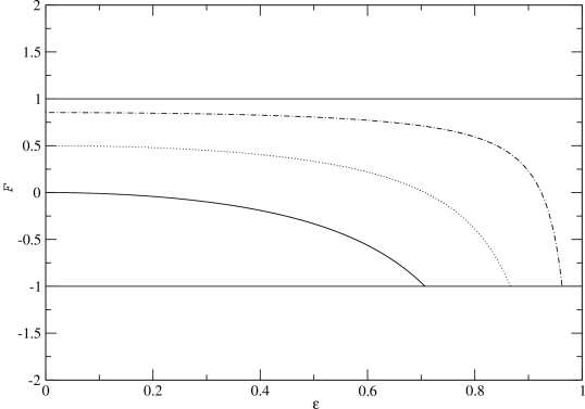
Figure 1: The allowed values of $m_{Z^{\prime}}$ for $\phi=\pi/8$ (dash-dot), $\phi=\pi/4$ (dash) and $\phi=\pi/2$ (solid).

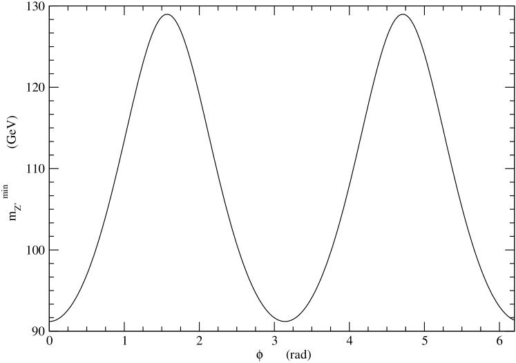
Figure 2: The minimum values for $m_{Z^{\prime}}$.

A $4\times 4$ orthogonal matrix ${\cal O}$ can be obtained such that it diagonalizes (12) and transforms the basis, connecting physical fields $F_{\mu}=(A^{\prime}_{\mu},Z^{\prime}_{\mu},Z_{\mu},A_{\mu})$ with $V_{\mu}$

$$V_{\mu}={\cal O}\,F_{\mu}\,.$$ (22)

Considering parametrization (14) and the following

$$\tan{\eta} = \frac{g_{C}}{g_{Y}}\cos{\phi}$$

$$\tan{\theta} = \frac{g_{Y}^{\prime}}{g_{2}}=\frac{g_{Y}}{g_{2}}\sec{\eta}$$

$$\tan{\psi} = \frac{m_{W}^{2}\sin{\eta}\tan{\phi}\sin{\theta}}{m_{W}^{2}-m^{2}_{Z^{\prime}}\cos^{2}{\theta}}$$ (23)

with $g_{Y}^{\prime}=\sqrt{g_{Y}^{2}+g_{C}^{2}\cos{\phi}^{2}}$, the ${\cal O}$ matrix can be determined in terms of these quantities, such that

$${\cal O}=\left(\begin{array}[]{cccc}c_{\eta}s_{\phi}&c_{\phi}c_{\psi}+s_{\eta}s_{\phi}s_{\psi}s_{\theta}&c_{\phi}s_{\psi}-c_{\psi}s_{\eta}s_{\phi}s_{\theta}&-c_{\theta}s_{\eta}s_{\phi}\\ -c_{\eta}c_{\phi}&c_{\psi}s_{\phi}-c_{\phi}s_{\eta}s_{\psi}s_{\theta}&s_{\phi}s_{\psi}+c_{\phi}c_{\psi}s_{\eta}s_{\theta}&c_{\phi}c_{\theta}s_{\eta}\\ s_{\eta}&-c_{\eta}s_{\psi}s_{\theta}&c_{\eta}c_{\psi}s_{\theta}&c_{\eta}c_{\theta}\\ 0&c_{\theta}s_{\psi}&-c_{\psi}c_{\theta}&s_{\theta}\end{array}\right)\,,$$ (28)

(29)

with $c_{\theta}=\cos{\theta}$, $s_{\theta}=\sin{\theta}$ etc. The transformed fields are written as

$$X_{\mu} = c_{\eta}s_{\phi}A^{\prime}_{\mu}+(c_{\phi}c_{\psi}+s_{\eta}s_{\phi}s_{\psi}s_{\theta})Z^{\prime}_{\mu}+(c_{\phi}s_{\psi}-c_{\psi}s_{\eta}s_{\phi}s_{\theta})Z_{\mu}-c_{\theta}s_{\eta}s_{\phi}A_{\mu}$$

$$C_{\mu} = -c_{\eta}c_{\phi}A^{\prime}_{\mu}+(c_{\psi}s_{\phi}-c_{\phi}s_{\eta}s_{\psi}s_{\theta})Z^{\prime}_{\mu}+(s_{\phi}s_{\psi}+c_{\phi}c_{\psi}s_{\eta}s_{\theta})Z_{\mu}+c_{\phi}c_{\theta}s_{\eta}A_{\mu}$$

$$B_{\mu} = s_{\eta}A^{\prime}_{\mu}-c_{\eta}s_{\psi}s_{\theta}Z^{\prime}_{\mu}+c_{\eta}c_{\psi}s_{\theta}Z_{\mu}+c_{\eta}c_{\theta}A_{\mu}$$

$$W_{\mu}^{3} = c_{\theta}s_{\psi}Z^{\prime}_{\mu}-c_{\psi}c_{\theta}Z_{\mu}+s_{\theta}A_{\mu}.$$ (30)

The derivative defined in (3b) can be written using (30)

$$D_{\mu}=\partial_{\mu}+\frac{i}{2}\,\left(\alpha_{1}\,A^{\prime}_{\mu}+\alpha_{2}\,A_{\mu}+\alpha_{3}\,Z^{\prime}_{\mu}+\alpha_{4}\,Z_{\mu}\right)$$ (31)

where

$$\alpha_{1} = 0$$

$$\alpha_{2} = e\,Q_{em}$$

$$\alpha_{3} = g_{2}\,s_{\psi}\,c_{\theta}\,\tau^{\,3}-\left[\,\frac{}{}g_{Y}\,c_{\eta}\,s_{\psi}\,s_{\theta}\,-g_{C}\,\left(s_{\phi}\,c_{\psi}-c_{\phi}\,s_{\psi}\,s_{\eta}\,s_{\theta}\,\right)\right]\,Y$$

$$\alpha_{4} = -g_{2}\,c_{\psi}\,c_{\theta}\,\tau^{\,3}+\left[\,\frac{}{}g_{Y}\,c_{\eta}\,c_{\psi}\,s_{\theta}\,+g_{C}\,\left(s_{\phi}\,s_{\psi}+c_{\phi}\,c_{\psi}\,s_{\eta}\,s_{\theta}\,\right)\right]\,Y\,$$ (32)

with $Q_{em}\,=\,\tau^{\,3}/2+Y/2$ is the usual charge operator and the eletric charge is defined as

$$e = \frac{g_{Y}^{\prime}g_{2}}{\sqrt{g_{2}^{2}+(g_{Y}^{\prime})^{2}}}\,.$$ (33)

As a direct consequence of $\alpha_{1}=0$ in (32), the interaction of a dark photon field $A^{{}^{\prime}}_{\mu}$ with a SM model current $j_{\mu}$ has no contribution and guarantees no direct coupling between the dark photon and SM charged particles. The interaction Lagrangian in the dark sector, defined in (3a), can be written using (30) as

$$-{\cal L}^{\chi}_{\rm int} = g_{x}\,\left(\alpha_{5}\,A^{\prime}_{\mu}+\alpha_{6}\,A_{\mu}+\alpha_{7}\,Z^{\prime}_{\mu}+\alpha_{8}\,Z_{\mu}\right)\,j^{\mu}_{\chi}$$ (34)

where

$$\alpha_{5} = g_{x}\,c_{\eta}s_{\phi}\,Q_{x}$$

$$\alpha_{6} = -g_{x}\,c_{\theta}s_{\eta}s_{\phi}\,Q_{x}$$

$$\alpha_{7} = g_{x}\,(c_{\phi}c_{\psi}+s_{\eta}s_{\phi}s_{\psi}s_{\theta})\,Q_{x}$$

$$\alpha_{8} = g_{x}\,(c_{\phi}s_{\psi}-c_{\psi}s_{\eta}s_{\phi}s_{\theta})\,Q_{x}\,.$$ (35)

The coupling of the photon to the $\chi$ fermion of the dark sector results in a dark charge $e_{x}$

$$e_{x}=g_{x}c_{\eta}s_{\phi}=\xi\,e$$ (36)

where

$$\xi=\frac{g_{x}g_{Y}}{g_{2}}\sin{\phi}\frac{\sqrt{g_{2}^{2}+g_{Y}^{2}+g_{C}^{2}\cos^{2}\phi}}{g_{Y}^{2}+g_{C}^{2}\cos^{2}\phi}.$$ (37)

To guarantee dark charge conservation, the dark photon has the same coupling to the $\chi$ fermion as the ordinary photon. The dark charge is dependent on the degree of mixture of the SM with the dark sector. In the case of $\phi=\pi/2$ one has $g_{Y^{\prime}}=g_{Y}$, using the known values $g_{2}\simeq 0.65$ and $g_{Y}\simeq 0.35$, Eq. (37) simplifies to

$$\xi=g_{x}\,\frac{\sqrt{g_{2}^{2}+g_{Y}^{2}}}{g_{Y}\,g_{2}}\,\,\simeq\,\,3.2\,\,g_{x}.$$ (38)

If the coupling $g_{x}$ is small, for example, the same order of $g_{C}$, then the dark electric charge is a fractional milli-charge, $e_{x}\sim 10^{-3}\,e$ . Historically, the context of milli-charged dark matter was first discussed by Holdom holdom , Goldberg and Hall goldberg and in recent studies taiwan -zp . In summary, these studies have shown that milli-charged particles, with fractional electric charge ranging from $10^{-6}$ to $10^{-1}$ of a unit charge are allowed.

III An astrophysical application

III.1 Stellar energy loss

Astrophysical observations have become a well-known tool to obtain empirical constraints on new particles. Any light particle, in principle, has a potential for playing an important role in stellar energy loss. Such a particle would remove energy from the stellar thermal bath by a direct mechanism. If stellar matter has a sufficient content of dark matter, an important process to consider, is the $\gamma^{\prime}$ emission from thermal states. This is relevant for determining the relic cosmological abundance, but is also the source of important constraints arising from new energy-loss mechanisms in stars. To obtain an estimate of the impact on stellar cooling, we will focus on the Compton-like process $\chi+\gamma\to\chi+\gamma^{\prime}$ by the diagrams in figure (3). The energy loss is given by $Q_{\gamma^{\prime}}$

$$Q_{\gamma^{\prime}}=\frac{1}{\rho}\int\frac{d^{3}q_{\gamma}}{(2\pi)^{3}}\frac{2}{e^{\omega\beta}-1}\int\frac{d^{3}q_{\chi}}{(2\pi)^{3}}\frac{2}{e^{E_{\chi}\beta}+1}\,\,\,\sigma_{c}\,E_{f}\,\,$$ (39)

where $\omega$ is photon energy in the thermal bath; $E_{\chi}$ is the energy of the fermions of the dark sector; $E_{f}$ is the star’s energy loss due to the dark photons and $\sigma_{c}$ is the Compton cross section of the processes. The total cross-section for dark photon production from Compton scattering is

$$\sigma_{c} = \pi\frac{(\xi^{2}\alpha)^{2}}{m_{\chi}}\Bigg{[}\frac{4m_{\chi}}{\omega^{2}}+\left.2\frac{(m_{\chi}+\omega)}{(m_{\chi}+2\omega)^{2}}-\frac{1}{\omega^{3}}(2m_{\chi}^{2}+2m_{\chi}\omega-\omega^{2})\ln\left({1+\frac{2\omega}{m_{\chi}}}\right)\right].$$ (40)

To evaluate $Q_{\gamma^{\prime}}$ in (39), one can use the following: $E_{f}\approx\omega$, $d^{3}q_{\gamma}=dk|\vec{k}|^{2}d\Omega$, $d^{3}q_{\chi}=dp|\vec{p}|^{2}d\Omega$, $dk=d\omega$, $dp=(E_{\chi}/|\vec{p}|)dE_{\chi}$, $\omega^{2}=|\vec{k}|^{2}$ and $|\vec{p}|^{2}=E_{\chi}^{2}-m_{\chi}^{2}$. The energy loss becomes

$$Q_{\gamma^{\prime}} = \frac{1}{\rho}\frac{1}{(2\pi)^{6}}\int_{0}^{\infty}(8\pi)d\omega\frac{\omega^{3}}{e^{\omega\beta}-1}\int_{m_{\chi}}^{\infty}(8\pi)dE_{\chi}\sqrt{E_{\chi}^{2}-m_{\chi}^{2}}\frac{E_{\chi}}{e^{E_{\chi}\beta}+1}\,\sigma_{c}\,.$$ (41)

We approximate $\sigma_{c}$ as a constant when compared to the integral of $E_{\chi}$, which results in

$$Q_{\gamma^{\prime}}=\frac{m_{\chi}^{5}(\xi^{2}\alpha)^{2}}{\rho\pi^{3}}\,I_{1}\,I_{2}$$ (42)

where

$$I_{1} = \int_{0}^{\infty}\frac{dx}{e^{\beta\,m_{\chi}\,x}-1}\,f(x)$$

$$I_{2} = \int_{1}^{\infty}dx\,\sqrt{x^{2}-1}\,\frac{x}{e^{\beta\,m_{\chi}\,x}+1}$$ (43)

with

$$f(x)=4x+\frac{2x^{3}(1+x)}{(1+2x)^{2}}-(2+2x-x^{2})\ln(1+2x)\,.$$

In order to establish a comparison of our results with other stellar cooling mechanisms we shall consider two known cases: axions in white dwarfs and neutrinos in protoneutron stars.

The axion was originally introduced as a very light dark matter candidate, where the supernova 1987A dynamics and laboratory searches has constrained its mass to values $\lesssim 0.01$ eV. The main processes for axion emission are the Compton-type, the Primakoff process and the annihilation process axion0 -axion3 . The comparison with the present calculation (42) is established considering an axion Compton process $e+\gamma\rightarrow e+a$, extracted from axion0

$$Q_{a}=5.29\times 10^{4}\frac{1}{\mu_{e}}\,T_{8}^{\,6}\,I(T_{8},\rho)\,\left(\frac{m_{a}}{{\rm eV}}\right)^{2}\,,$$ (44)

with (44) in ergs/g sec; $T_{8}$ the temperature in units of $10^{8}$ K; $m_{a}$ the axion’s mass. The factor $I$ is tabulated in Appendix A of axion0 , where $I=1$ is the nonrelativistic and nondegenerate limit.

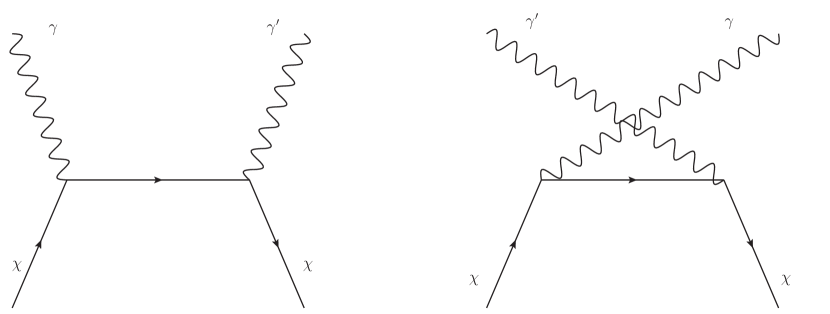
Figure 3: Compton diagrams

As discussed in axion0 , if an axion with mass $m_{a}$ of 1 eV exists, the nuclear energy generation should be more than a hundred times larger and then the time scale of evolution becomes shorter by that factor. This effect should disturb the star distribution in the horizontal branch, therefore this mass value can be considered as an upper bound. By this fact, the value of $1$ eV is used as one of the reference masses in the axion energy loss calculation.

The characteristic signatures of dark matter are potentially detectable with the analysis of the stellar oscillations. Asteroseismology is presently showing its power in determining with high precision not only the global properties of stars but also their internal structure. Recently, A. H. Córsico et al. used the state-of-the-art asteroseimological model corsico1 to study the rate of the anomalous cooling of the pulsating white dwarf star G117-B15A. From this measure they inferred the axion mass due to this extra cooling mechanism and obtained the value of $m_{a}\cos^{2}\beta=17.4_{-2.7}^{+2.3}$ meV, where $\cos^{2}\beta$ is a free, model-dependent parameter that is usually set equal to unity corsico2 .

The energy loss is density dependent quantity, therefore a $Q$ calculation involves an estimate of ordinary stellar matter density, which is very well established for axions or neutrinos, both coupling to SM fields. Due to the restrictions imposed by Eq. (32) ($\alpha_{1}=0$) on direct interactions of dark photons with ordinary SM charged particles, a $\gamma\leftrightarrow\gamma^{\prime}$ conversion must always involve a dark $\chi$ fermion. A $Q$ calculation in this scenario implies in a rough estimate of the dark matter density. On distance scales of the size of galaxies and clusters of galaxies, evidence of dark matter are compelling, but still observations do not allow one to determine the total amount of dark matter in the Universe. Information has been extracted from the analysis of the cosmic microwave background (CMB). In particular, stringent constraints on the abundances of baryons and matter in the Universe has been placed by the Wilkinson microwave anisotropy probe (WMAP) data and recently by high resolution detections of both the total intensity and polarization of primordial CMB anisotropies by Planck planck . $N$-body simulations suggest the existence of a universal dark matter profile for halo densities, where some of the most widely used profile models are Kravtsov et al. profile1 , Navarro, Frenk and White profile2 , Moore et al. profile3 and modified isothermal profile4 profiles. Therefore, if dark matter can be assigned as a constituent of stellar interiors, in a first approximation, a conservative choice for the unknown stellar density is to assume that it matches the density of ordinary stellar matter. This is consistent with recent studies where ordinary stellar matter is mixed with non-self-annihilating dark matter mix1 ; mix2 . It was found that a more compact star results when a DM core is included. Dark matter density profiles are presented showing a high density dark matter stellar core. As will be shown, this is sufficient for the dark photon mechanism to be comparable with other known cooling mechanisms.

III.2 Astrophysical constraints

Stellar density, assumed to be made of pure hydrogen, ranges from $10^{2}\lesssim\rho\lesssim 10^{4}$ g$\cdot$cm^-3 which is, typically the range for a star like the Sun to a red giant. Compact stars like white dwarfs, have higher densities of matter, of order $10^{6}$ g$\cdot$cm^-3 and temperatures of $10^{7}$ K. In the temperature range around $10^{8}$ K, the Compton-type process (44) is dominant axion0 -axion3 .

The input parameters for the energy loss $Q$ are set for two initial densities as $\rho\sim 10^{4}$ g$\cdot$cm^-3 (typical red giant) and $\rho\sim 10^{6}$ g$\cdot$cm^-3 (typical white dwarf). The millicharge is fixed at $\xi=10^{-3}$ and $\alpha=1/137$. The two axion reference masses $m_{a}$ are 1 eV and 1 meV. For the first case, as can be seen in figure (4) for both densities, the Compton scattering of dark photons off a fermion singlet results in $Q_{\gamma^{\prime}}$ comparable to the axion $Q_{a}$ for masses $m_{\chi}$ of 1 eV, 10 eV and 1 keV. In particular, for the typical white dwarf temperature zone ($T\sim 10^{7}$ K), the energy loss from axion Compton scattering is comparable to a dark photon scattered off a very light fermion singlet of $m_{\chi}=10$ eV. In the second case, the extremely light axion produces, for both densities, lower $Q_{a}$ curves, which implies that for a comparable $Q_{\gamma^{\prime}}$ , as seen in figure (5), the fermion singlet masses $m_{\chi}$ must be smaller. Again, for the typical white dwarf temperature zone the dark fermion must have a mass of 0.5 eV.

As well known the window with charges of order $\xi=10^{-2}$ is opened in the models with paraphotons only, when the relic density of these particles is suppressed by annihilation art1 ; art2 . In our model we can test the sensitivity of the energy loss mechanism to the millicharge and fermion masses for white dwarfs. Figure (7), where one defines $\eta=\log\xi$, shows that in a region consistent with typical white dwarf temperatures of $10^{7}$ K to $10^{8}$ K the most significant energy loss for a light mass singlet of 1 eV is for $\xi=10^{-3}$ to $\xi=10^{-2}$. In the same region there is an overlap with a heavier fermion of 1 keV, where a new interval of smaller millicharges is accepted from $\xi=10^{-5}$ to $\xi=10^{-4}$. For this mass of 1 keV the most important contributions for a possible energy loss occurs at edge of the charge window at $\xi=10^{-2}$. A heavier fermion of 1 MeV is out of the typical white dwarf temperature range and no effect would be expected.

Effects of dark photons on higher density and temperature zones can also be probed in supernovas, where typical densities are of the order $\rho\sim 10^{14}$ g$\cdot$cm^-3 and temperatures, inside a newly formed neutron star, are $T\sim 10^{12}$ K. The detection of neutrinos from SN 1987A confirmed that the almost $3\times 10^{53}$ ergs of gravitational energy gained by the core collapse are emitted as neutrino radiation on time scales of tens of seconds, during which the central protoneutron star (PNS) cools, deleptonizes, and contracts sn1 ; sn2 . In present model a very crude luminosity estimate can be made considering a homogeneous 15 $M_{\odot}$ progenitor sn2 ; sn3 . As shown in Eq. (32) there is no direct coupling between the dark photon and SM charged particles, resulting that ordinary stellar matter is transparent for dark photons. Dark photons, again, could be an alternative cooling mechanism for dense matter in the neutron star regime. In the white dwarf problem the mass range for $m_{\chi}$ is too restrictive and implies in an extremely light WIMP option. For matter at neutron star densities our model admits a heavier WIMP, as seen in figure (6), which is consistent with the mass of the dark matter candidates from DAMA/LIBRA dama-libra and CoGeNT cdms observations.

A challenging issue is to find a unifying scenario in which both “white dwarf WIMPS” and “supernova WIMPS” can coexist with a consistent set of parameters. As can be seen in figures (4)-(6) there is a clear starting temperature, a $Q$-threshold, which is strongly dependent on the $\chi$ mass. If a very light $\chi$ ($m_{\chi}\approx 10$ keV) is present in a supernova it will have a $Q$-threshold at temperatures of $T\sim 10^{6}$ K, which is many orders below usual protoneutron star temperatures. To play a significant role in the energy loss mechanism, implies that $\chi$ has a larger mass, as can be seen in figure (6). A similar WIMP exclusion occurs for a heavy $\chi$ ($m_{\chi}\approx 10$ GeV) in a white dwarf. The $Q$-threshold will occur at temperatures of $T\sim 10^{12}$ K, again many orders above usual white dwarf temperatures. Therefore by this simple analysis a unifying scenario can be obtained if one introduces two species of dark fermions $\chi_{1}$ and $\chi_{2}$ in (2c) with masses $m_{\chi_{1}}\ll m_{\chi_{2}}$.

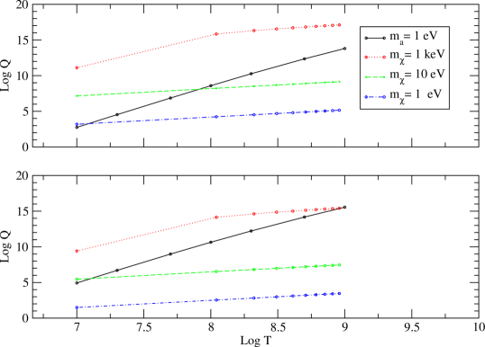
Figure 4: Comparison of the energy loss for an axion of mass $m_{a}$=1 eV and a fermion singlet $\chi$ : $\rho\sim 10^{4}$ g/cm³ (upper), $\rho\sim 10^{6}$ g/cm³ (lower). Q in ergs/g.sec and T in K.

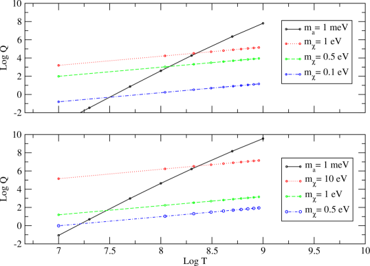
Figure 5: Comparison of the energy loss for an axion of mass $m_{a}$=1 meV and a fermion singlet $\chi$ : $\rho\sim 10^{4}$ g/cm³ (upper), $\rho\sim 10^{6}$ g/cm³ (lower). Q in ergs/g.sec and T in K.

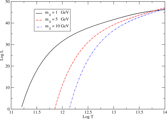
Figure 6: Average dark photon luminosity for the fermion singlet, with masses $m_{\chi}=1$, 5, 10 GeV and $\rho\sim 10^{14}$ g/cm³. L in ergs/sec and T in K.

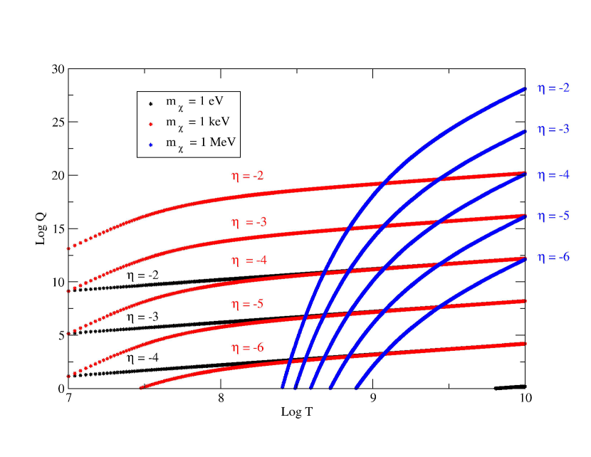
Figure 7: Energy loss for fermion singlets $\chi$ of different masses and millicharges: $\rho\sim 10^{6}$ g/cm³. Q in ergs/g.sec, T in K and $\eta=\log\xi$

IV Conclusions

We have studied some consequences of an extension of the Standard Model in a hybrid scenario where two new $U(1)$ vector bosons were introduced. The first boson $C_{\mu}$ coupled to the SM by the usual minimal coupling, producing an enlarged gauge sector in the SM, acquiring mass by the Higgs mechanism, and a second boson $X_{\mu}$ mixed with $C_{\mu}$ via Stueckelberg coupling. After symmetry breaking, four physical bosons were present, two massive: $Z$, $Z^{\prime}$ and two photon-like $\gamma$ and $\gamma^{\prime}$ (dark photon). There is a extensive literature on extra $U(1)$ gauge bosons that appear in the context of many models such as $SO(10)$ or $E_{6}$, string and D-brane models and many other different schemes hewett -dm2 . Still, the cleanest signatures for a new $Z^{\prime}$ boson would be mass peak in a resonant production in $e^{+}e^{-}$ collision. As reported recently by the CMS Collaboration, a search for narrow resonances was carried out in dimuon and dielectron invariant mass spectra in event samples corresponding to an integrated luminosity of $20.6$ fb^-1 for dimuons and $19.6$ fb^-1 for dielectrons ($\sqrt{s}=8$ TeV) cms2 . The spectra they found was consistent with expectations from the SM, setting mass limits on neutral gauge bosons using the measured dilepton spectra. In this sense, a $Z^{\prime}$ with Standard Model-like couplings has been excluded below $2960$ GeV and the superstring-inspired below $2600$ GeV. These results are not in contradiction with the present model, for example Eq. (17), sets the minimum $Z^{\prime}$ mass value. In particular for $\phi=\pi/2$ (largest minimum value) the $Z^{\prime}$ mass must satisfy $m_{Z^{\prime}}>128.97$ GeV.

Direct measurements of dark photons $\gamma^{\prime}$ are hopeless due to the fact that $\hat{\alpha}_{1}=0$ in (31). A possible scenario in which a dark photon could be important would be in stellar cooling. A Compton-like diagram is present in the model converting $\gamma\leftrightarrow\gamma^{\prime}$ , similar to axion models where $\gamma\leftrightarrow a$, and could be used to estimate the impact in stellar cooling as an alternative mechanism. The comparison of $Q_{\gamma^{\prime}}$ and $Q_{a}$ , for white dwarfs, revealed that for an extremely light WIMP an “overlap zone” is possible in which both mechanisms are of the same order and, in principle, could both contribute to stellar energy loss.

There have been light-mass WIMP claims that report an excess of low-energy events relative to expected backgrounds, the so called annual modulation effect, from CoGeNT collaboration. This excess, if interpreted as dark matter, implies that dark matter particles possess a mass in the range of 5 to 15 GeV cogent and in a recent study a mass of 7 GeV was obtained cogent2 . The DAMA/LIBRA collaboration has presented similar results which are consistent with the CoGeNT dark matter observations dama-libra . In the opposite direction of these direct measurements reports, the CDMS collaboration has recently claimed to exclude a light-WIMP interpretation of CoGeNT and DAMA/LIBRA observations cdms . Observations from XENON10 and XENON100 have been used to establish a similar rejection of light-WIMP scenarios xenon1 ; xenon2 . Recent results from LUX (Large Underground Xenon experiment), have shown to be consistent with the background-only hypothesis setting a 90% confidence limit on spin-independent WIMP-nucleon elastic scattering. A minimum upper limit on the cross section of 7.6 $\times 10^{-46}$ cm² at a WIMP mass of 33 GeV is presented lux . Similar to other xenon based experiments, the LUX data is in strong disagreement with low-mass WIMP signal interpretations of the results from several recent direct detection experiments.

The mass of our “white dwarf WIMP” is far below the measured values in these experiments. In fact, for the energy loss mechanism, formerly described, to take place, the dark matter fermion singlet must be lighter than an electron ($m_{\chi}\ll m_{e}$ ). In a typical Bhabha scattering, for example, there should be sufficient energy in the annihilation diagram to produce, in the final state, $e^{+}e^{-}$ and $\bar{\chi}\chi$. By this argument these extremely light dark fermions should be abundantly produced. Now, a simple comparison of the $e^{+}e^{-}\rightarrow\bar{\chi}\chi$ cross section with the $e^{+}e^{-}\rightarrow e^{+}e^{-}$ annihilation cross section in the limit $\sqrt{s}\gg 2m_{e}$,

$$\frac{\sigma_{e^{+}e^{-}\rightarrow\bar{\chi}\chi}}{\sigma^{ann}_{e^{+}e^{-}\rightarrow e^{+}e^{-}}}\simeq\xi^{2},$$

showing a strong suppression of $\chi$ production.

Alternatively, we have shown that the “supernova WIMP” has a mass range of a few GeV, consistent with the claimed light-WIMP candidates and resulting in an energy-loss of the order of neutrino cooling. This could be a promising path for future calculations. A unifying scenario where both neutron star constraints and white dwarf constraints are consistent implies in introducing two species of fermions $\chi_{1}$ and $\chi_{2}$ in ${\cal L}_{\chi}$ with masses $m_{\chi_{1}}\ll m_{\chi_{2}}$.

References

- (1) G. Bertone, D. Hooper and J. Silk, Particle dark matter: evidence, candidates and constraints, Phys. Rep. 405, 279 (2005) [arXiv:hep-ph/0404175].
- (2) G. Jungman, M. Kamionkowski and K. Griest, Phys. Rept. 267 195, (1996) [arXiv:hep-ph/9506380].
- (3) S. Dodelson and L. M. Widrow, Phys. Rev. Lett. 72 17, (1994) [arXiv:hep-ph/9303287].
- (4) N. Arkani-Hamed, A. G. Cohen and H. Georgi, Phys. Lett. B 513 232, (2001) [arXiv:hep-ph/0105239].
- (5) N. Arkani-Hamed, A. G. Cohen, T. Gregoire and J. G. Wacker, JHEP 08 020, (2002) [arXiv:hep-ph/0202089].
- (6) N. Arkani-Hamed, A. G. Cohen, E. Katz and A. E. Nelson, JHEP 07 034, (2002) [arXiv:hep-ph/0206021].
- (7) K. Agashe and G. Servant, Phys. Rev. Lett. 93 231805, (2004) [arXiv:hep-ph/0403143].
- (8) N. Arkani-Hamed, D. P. Finkbeiner, T. R. Slatyer and N. Weiner, Phys. Rev. D 79 015014, (2009) [arXiv:0810.0713].
- (9) B. W. Lee and S. Weinberg, Phys. Rev. Lett. 39 165, (1977).
- (10) C. Boehm, D. Hooper, J. Silk, M. Casse, J. Paul, Phys. Rev. Lett. 92 101301, (2004) [arXiv:astro-ph/0309686].
- (11) P. Langacker, Rev. Mod. Phys. 81 1199, (2009) [arXiv:0801.1345].
- (12) B. A. Dobrescu, Phys. Lett. B 403 285, (1997) [arXiv:hep-ph/9703390].
- (13) B. A. Dobrescu, Phys. Rev. Lett. 94 151802, (2005) [arXiv:hep-ph/0411004].
- (14) B. Holdom, Phys. Lett. B 178 65, (1986).
- (15) D. A. Demir, G. L. Kane, T. T. Wang, Phys. Rev. D 72 015012, (2005) [arXiv:hep-ph/0503290].
- (16) P. Batra, B. A. Dobrescu, D. Spivak, J. Math. Phys. 47 082301, (2006) [arXiv:hep-ph/0510181].
- (17) M. Williams, C.P. Burgess, A. Maharana, F. Quevedo, JHEP 1108 106, (2011) [arXiv:1107.0882].
- (18) B. Körs and P. Nath, JHEP 07 069, (2005) [arXiv:hep-ph/0503208].
- (19) ATLAS Collaboration, JHEP 11 138, (2012) [arXiv:1209.2535].
- (20) CMS Collaboration, Phys. Lett. B 720 63, (2013).
- (21) R. D. Peccei and H. R. Quinn, Phys. Rev. D 16 1791, (1977) .
- (22) N. G. Deshpande and E. Ma, Phys. Rev. D 18, 2574 (1978).
- (23) R. Barbieri, L. J. Hall and V. S. Rychkov, Phys. Rev. D 74 015007, (2006).
- (24) M. Aoki, S. Kanemura and O. Seto, Phys. Rev. Lett. 102 051805, (2009);
- (25) M. Aoki, S. Kanemura and O. Seto, Phys. Rev. D 80 033007 (2009).
- (26) H. S. Goh, L. J. Hall and P. Kumar, JHEP05 097, (2009).
- (27) Y. Baia and J. Berger JHEP11 171, (2013).
- (28) K. Cheung and T. C. Yuan, JHEP 03 120, (2007) [arXiv:hep-ph/0701107].
- (29) J. Beringer et al. (Particle Data Group), Review of Particle Physics Phys. Rev. D 86 010001, (2012).
- (30) D. Feldman, Z. Liu and P. Nath, Phys. Rev. Lett. 97 021801, (2006) [arXiv:hep-ph/0603039].
- (31) H. Goldberg and L. J. Hall, Phys. Lett. B 174 151, (1986).
- (32) M. Fukugita, S. Watamura and M. Yoshimura, Phys. Rev. D 26 1840, (1982).
- (33) D. A. Dicus, E. W. Kolb, V. L. Teplitz and R. V. Wagoner, Phys. Rev. D 22 839, (1980).
- (34) J. A. Grifols and E. Masso, Phys Lett. B 173 237, (1986).
- (35) G. Raffelt and A. Weiss, Phys. Rev. D 51 1495, (1995) [arXiv:hep-ph/9410205].
- (36) A. H. Córsico, O. G. Benvenuto, L. G. Althaus, J. Isern and E. García-Berro, New Astron. 6 197, (2001) [arXiv:astro-ph/0104103].
- (37) A. H. Córsico, L. G. Althaus, M. M. Miller Bertolami, A. D. Romero, García-Berro, J. Isern and S. O. Kepler, Mon. Not. R. Astron. Soc. 424 2792, (2012) [arXiv:1205.6180].
- (38) Planck Collaboration: P. A. R. Ade et al., Astron. and Astroph. 557 A52, (2013).
- (39) A. V. Kravtsov, A. A. Klypin, J. S. Bullock, J. R. Primack, Astrophys. J. 502 48, (1998) [arXiv:astro-ph/9708176].
- (40) J. F. Navarro, C. S. Frenk, S. D. White, Astrophys. J. 462 563, (1996) [arXiv:astro-ph/9508025].
- (41) B. Moore, T. Quinn, F. Governato, J. Stadel, G. Lake, Mon. Not. Roy. Astron. Soc. 310 1147, (1999) [arXiv:astro-ph/9903164].
- (42) L. Bergstrom, J. Edsjo, P. Ullio, Phys. Rev. D 58 083507, (1998) [arXiv:astro-ph/9804050].
- (43) S.-C. Leung, M.-C. Chu, L.-M. Lin, Phys. Rev. D 85 103528, (2012) [arXiv:1205.1909].
- (44) S.-C. Leung, M.-C. Chu, L.-M. Lin, K.-W. Wong, Phys. Rev. D 87 123506, (2013) [arXiv:1305.6142].
- (45) S. E. Woosley, A. Heger, T. A. Weaver, Rev. Mod. Phys. 74 1015, (2002).
- (46) H. Vogel, J. Redondo, JCAP 1402 029 (2014).
- (47) A. D. Dolgov, S. L. Dubovsky, G. I. Rubtsov, and I. I. Tkachev Phys.Rev. D88 11, 117701 (2013).
- (48) G. Martinez-Pinedo, T. Fischer, A. Lohs, L. Huther, Phys. Rev. Lett. 109 251104, (2012) [arXiv:1205.2793].
- (49) M. I. Vysotsskii, Ya. B. Zel’dovich, M. Yu. Khlopov, V. M. Chechetkin, JETP Lett. 27 502, (1978).
- (50) R. Bernabei, P. Belli, F. Cappella et al., Eur. Phys. J. C 67 39, (2010) [arXiv:1002.1028].
- (51) Z. Ahmed et al., Phys. Rev. Lett. 106 131302, (2011) [arXiv:1011.2482].
- (52) J. L. Hewett, T.G. Rizzo, Phys. Rep. 183 193, (1989).
- (53) M. Cvetic, P. Langacker, Phys. Rev. D 54 3570, (1996) [arXiv:hep-ph/9511378].
- (54) V. D. Barger, K. M. Cheung, P. Langacker, Phys. Lett. B 381 226, (1996) [arXiv:hep-ph/9604298].
- (55) B. Körs and P. Nath, Phys Lett. B 586 366, (2004) [arXiv:hep-ph/0402047].
- (56) D. Feldman, B. Körs and P. Nath, Phys. Rev. D 75 023503, (2007) [arXiv:hep-ph/0610133].
- (57) D. Feldman, Z. Liu, P. Nath and G. Peim, Phys. Rev. D 81 095017, (2010) [arXiv:1004.0649].
- (58) CMS Collaboration, CMS Physics Analysis Summary, CMS-PAS-EXO-12-061 (2013).
- (59) D. Hooper, J. I. Collar, J. Hall, D. McKinsey and C. M. Kelso, Phys. Rev. D 82 123509, (2010) [arXiv:1007.1005].
- (60) C. E. Aalseth, et al., Phys. Rev. Lett. 107 141301, (2011) [arXiv:1106.0650].
- (61) E. Aprile et al., Phys. Rev. Lett. 107 131302, (2011) [arXiv:1104.2549].
- (62) J. Angle et al., Phys. Rev. Lett. 107 051301, (2011) [arXiv:1104.3088].
- (63) D. S. Akerib et al., Phys. Rev. Lett. 112 0913030, (2014) [arXiv:1310.8214].