Almost sure optimal hedging strategy

Abstract

In this work, we study the optimal discretization error of stochastic integrals, in the context of the hedging error in a multidimensional Itô model when the discrete rebalancing dates are stopping times. We investigate the convergence, in an almost sure sense, of the renormalized quadratic variation of the hedging error, for which we exhibit an asymptotic lower bound for a large class of stopping time strategies. Moreover, we make explicit a strategy which asymptotically attains this lower bound a.s. Remarkably, the results hold under great generality on the payoff and the model. Our analysis relies on new results enabling us to control a.s. processes, stochastic integrals and related increments.

and T1This research is part of the Chair Financial Risks of the Risk Foundation, the Chair Derivatives of the Future and the Chair Finance and Sustainable Development.

1 Introduction

The problem. We aim at finding a finite sequence of optimal stopping times ${\mathcal{T}}^{n}=\{\tau^{n}_{0}=0<\tau^{n}_{1}<\cdots<\tau^{n}_{i}<\cdots<\tau^{n}_{{N^{n}_{T}}}=T\}$ which minimizes the quadratic variation of the discretization error of the stochastic integral

$$Z_{s}^{n}=\int_{0}^{s}D_{x}u(t,S_{t})\cdot\,\mathrm{d}S_{t}-\sum_{\tau^{n}_{i-1}\leq s}D_{x}u\bigl{(}{\tau^{n}_{i-1}},S_{\tau^{n}_{i-1}}\bigr{)}\cdot(S_{\tau^{n}_{i}\land s}-S_{\tau^{n}_{i-1}}),$$

which interpretation is the hedging error bert:koga:lo:00 of the discrete Delta-hedging strategy of a European option with underlying asset $S$ (multidimensional Itô process), maturity $T>0$, price function $u$ (for the ease of presentation, here $u$ depends only on $S$) and payoff $g(S_{T})$. The times $(\tau^{n}_{i})_{1\leq i\leq{N^{n}_{T}}}$ read as rebalancing dates (or trading dates), and their number ${N^{n}_{T}}$ is a random variable which is finite a.s. The exponent $n$ refers to a control parameter introduced later on; see Section 2. The a.s. minimization of $Z^{n}_{T}$ is hopeless since after a suitable renormalization, it is known that it weakly converges to a mixture of Gaussian random variables (see bert:koga:lo:00 , GT01 , HM05 , GT09 when trading dates are deterministic and under some mild assumptions on the model and payoff; see fuka:11 for stopping times under stronger assumptions). Hence it is more appropriate to investigate the a.s. minimization of the quadratic variation $\langle Z^{n}\rangle_{T}$ which, owing to the Lenglart inequality (resp., the Burkholder–Davis–Gundy inequality), allows the control of the distribution (resp., the $L_{p}$-moments, $p>0$) of $\sup_{t\leq T}|Z^{n}_{t}|$ under martingale measure. To avoid trivial lower bounds by letting ${N^{n}_{T}}\rightarrow+\infty$, we reformulate our problem into the a.s. minimization of the product

$${N^{n}_{T}}\bigl{\langle}Z^{n}\bigr{\rangle}_{T}.$$ (1)

As emphasized in F11 , the resolution of this optimization problem allows the asymptotic minimization of more general costs of the form $C({N^{n}_{T}},\langle Z^{n}\rangle_{T})$, where the function $C\dvtx\mathbb{R}^{2}\mapsto\mathbb{R}$ is increasing in both variables. Our Theorem 3.1 states that the renormalized error (1) has a.s. an asymptotic lower bound over the class of admissible strategies which consist (roughly speaking) of deterministic times and of hitting times of random ellipsoids of the form

$$\hskip 6.0pt\qquad\tau^{n}_{0}:=0,\qquad\tau^{n}_{i}:=\inf\bigl{\{}t\geq\tau^{n}_{i-1}\dvtx(S_{t}-S_{\tau^{n}_{i-1}})\cdot H_{\tau^{n}_{i-1}}(S_{t}-S_{\tau^{n}_{i-1}})=1\bigr{\}}\land T,$$ (2)

where $(H_{t})_{0\leq t\leq T}$ is a measurable adapted positive-definite symmetric matrix process. It includes the Karandikar scheme K95 for discretization of stochastic integrals. In addition, in Theorems 3.2 and 3.3 we show the existence of a strategy of the hitting time form attaining the a.s. lower bound. The derivation of a central limit-type theorem for $Z^{n}$ is left to further research (see land:13 ), in particular because the verification of the criteria in fuka:11 is difficult to handle in our general setting.

Literature background. Our work extends the existing literature on discretization errors for stochastic integrals with deterministic time mesh, mainly considered with financial applications. Many works deal with hedging rebalancing at regular intervals of length $\Delta t_{i}=T/n$. In Zh99 and bert:koga:lo:00 , the authors show that $\mathbb{E}[\langle Z^{n}\rangle_{T}]$ converges to 0 at rate $n$ for payoffs smooth enough [this convergence rate originates to consider the product (1) as a minimization criterion]. However, in GT01 it is proved that the irregularity of the payoff may deteriorate the convergence rate: it becomes $n^{1/2}$ for digital call option. This phenomenon has been intensely analyzed by Geiss and his co-authors using the concept of fractional smoothness (see geis:geis:04 , gobe:makh:10 , GG11 , geis:geis:gobe:11 and references therein): by the choice of rebalancing dates suitably concentrated at maturity, we recover the rate $n$.

The first attempt to find optimal strategies with nondeterministic times goes back to MP99 : the authors allow a fixed number $n$ of random rebalancing dates, which actually solve an optimal multiple-stopping problem. Numerical methods are required to compute the solution. In F11 , Fukasawa performs an asymptotic analysis for minimizing the product $\mathbb{E}({N^{n}_{T}})\mathbb{E}(\langle Z^{n}\rangle_{T})$ (an extension to jump processes has been recently done in rose:tank:11 ). Under regularity and integrability assumptions (and for a convex payoff on a single asset), Fukasawa derives an asymptotic lower bound and provides an optimal strategy. His contribution is the closest to our current work. But there are major differences: [(1)]

We focus on a.s. results, which is probably more meaningful for hedging issues. We are not aware of similar works in this direction.

We allow a quite general model for the asset. It can be a multidimensional diffusion process (local volatility model); see the discussion in Section .8. As a comparison, in F11 the analysis is carried out for a one-dimensional model (mainly Black–Scholes model).

We also allow a great generality on the payoff. In particular, the payoff can be discontinuous, and the option can be exotic (Asian, lookback, …) (see Section .8 for examples): for mathematical reasons, this is a major difference in comparison with F11 . Indeed, in the latter reference, the payoff convexity is needed to ensure the positivity of the option Gamma (second derivative of price), which is a crucial property in the analysis. Also, for discontinuous payoff the $L_{p}$ integrability of the sensitivities (Greeks) up to maturity may be not satisfied (see gobe:makh:11 ); thus, some quantities in the analysis (e.g., the integral of the second moment of the Gamma of digital call option) may become infinite. In our setting, we circumvent these issues by only requiring the sensitivities to be finite a.s. up to maturity: actually, this property is systematically satisfied by payoffs for which the discontinuity set has a zero-measure (see Section .8), which includes all the usual situations to our knowledge. To achieve such a level of generality and an a.s. analysis, we design efficient tools to analyze the a.s. control and a.s. convergence of local martingales, of their increments and so forth. All these results represent another important theoretical contribution of this work. Other applications of these techniques are in preparation. At last, although the distribution of hitting time of random ellipsoid of the form (2) is not explicit, quite surprisingly we obtain tight estimates on the maximal increments of $\sup_{i\leq{N^{n}_{T}}}(\tau^{n}_{i}-\tau^{n}_{i-1})$, which may have applications in other areas (like stochastic simulation).

Outline of the paper. In the following, we present some notation and assumptions that will be used throughout the paper. Section 2 is aimed at defining our class of stopping time strategies and deriving some general theoretical properties in this class. For that, we establish new key results about a.s. convergence, which fit well our framework. All these results are not specifically related to financial applications. The main results about hedging error are stated and proved in Section 3. Numerical experiments are presented in Section 4, with a practical description of the algorithm to build the optimal sequence of stopping times (actually hitting times) and a numerical illustration regarding the exchange binary option (in dimension 2).

Notation used throughout the paper.

• We denote by $x\cdot y$ the scalar product between two vectors $x$ and $y$, and by $|x|=(x\cdot x)^{1/2}$ the Euclidean norm of $x$; the induced norm of a $m\times d$-matrix $A$ is denoted by $|A|:=\sup_{x\in\mathbb{R}^{d}\dvtx|x|=1}|Ax|$.

• $A^{*}$ stands for the transposition of the matrix $A$; $I_{d}$ stands for the identity matrix of size $d$; the trace of a square matrix $A$ is denoted by $\operatorname{Tr}(A)$.

• $\mathcal{S}^{d}(\mathbb{R})$, $\mathcal{S}_{+}^{d}(\mathbb{R})$ and $\mathcal{S}_{++}^{d}(\mathbb{R})$ are respectively the set of symmetric, symmetric nonnegative-definite and symmetric positive-definite $d\times d$-matrices with coefficients in $\mathbb{R}$: $A\in\mathcal{S}_{+}^{d}(\mathbb{R})$ [resp., $\mathcal{S}_{++}^{d}(\mathbb{R})$] if and only if $x\cdot Ax\geq 0$ (resp., $>0$) for any $x\in\mathbb{R}^{d}\setminus\{0\}$.

• For $A\in\mathcal{S}^{d}(\mathbb{R})$, $\Lambda(A):=(\lambda_{1}(A),\ldots,\lambda_{d}(A))$ stands for its spectrum (its $\mathbb{R}$-valued eigenvalues), and we set $\lambda_{\mathrm{min}}(A):=\min_{1\leq i\leq d}\lambda_{i}(A)$.

• For the partial derivatives of a function $f\dvtx(t,x,y)\mapsto f(t,x,y)$, we write $D_{t}f(t,x,y)=\frac{\partial f}{\partial t}(t,x,y)$, $D_{x_{i}}f(t,x,y)=\frac{\partial f}{\partial x_{i}}(t,x,y)$, $D_{x_{i}x_{j}}^{2}f(t,x,y)=\break\frac{\partial^{2}f}{\partial x_{i}\,\partial x_{j}}(t,x,y)$, $D^{2}_{x_{i}y_{j}}f(t,x,y)=\frac{\partial^{2}f}{\partial x_{i}\,\partial y_{j}}(t,x,y)$ and so forth.

• When convenient, we adopt the short notation $f_{t}$ in place of $f(t,S_{t},Y_{t})$ where $f$ is a given function and $(S_{t},Y_{t})_{0\leq t\leq T}$ is a continuous time process (introduced below).

• For a $\mathbb{R}^{d}$-valued continuous semimartingale $M$, $\langle M\rangle_{t}$ stands for the matrix of cross-variations $(\langle M^{i},M^{j}\rangle_{t})_{1\leq i,j\leq d}$.

• The constants of the multidimensional version of the Burkholder–Davis–Gundy inequalities KS91 , page 166, are defined as follows: for any $p>0$ there exists $c_{p}>1$ such that for any vector $M=(M^{1},\ldots,M^{d})$ of continuous local martingales with $M_{0}=0$ and any stopping time $\theta$, we have

  $$c^{-1}_{p}\mathbb{E}\Biggl{|}\sum_{j=1}^{d}\bigl{\langle}M^{j}\bigr{\rangle}_{\theta}\Biggr{|}^{p}\leq\mathbb{E}\Bigl{(}\sup_{t\leq\theta}|M_{t}|^{2p}\Bigr{)}\leq c_{p}\mathbb{E}\Biggl{|}\sum_{j=1}^{d}\bigl{\langle}M^{j}\bigr{\rangle}_{\theta}\Biggr{|}^{p}.$$ (3)

• For a given sequence of stopping times ${\mathcal{T}}^{n}$, the last time before $t\leq T$ is defined by $\varphi(t)=\max\{\tau^{n}_{j};\tau^{n}_{j}\leq t\}$: although dependent on $n$, we omit to indicate this dependency to alleviate notation. Furthermore, for a process $(f_{t})_{0\leq t\leq T}$, we write $\Delta f_{t}:=f_{t}-f_{\varphi(t-)}$ (omitting again the index $n$ for simplicity); in particular, we have $\Delta f_{\tau^{n}_{i}}=f_{\tau^{n}_{i}}-f_{\tau^{n}_{i-1}}$. Besides we set $\Delta_{t}=t-\varphi(t-)$ and $\Delta\tau^{n}_{i}:=\tau^{n}_{i}-\tau^{n}_{i-1}$.

• We shortly write $X^{n}\stackrel{{\scriptstyle a.s.}}{{\longrightarrow}}$ if the random variables $(X^{n})_{n\geq 0}$ converge almost surely as $n\rightarrow\infty$. We write $X^{n}\stackrel{{\scriptstyle a.s.}}{{\longrightarrow}}X^{\infty}$ to additionally indicate that the almost sure limit is equal to $X^{\infty}$. We shall say that the sequence $(X^{n})_{n\geq 0}$ is bounded if $\sup_{n\geq 0}|X^{n}|<+\infty$, a.s.

• $C_{0}$ is a a.s. finite nonnegative random variable, which may change from line to line.

Model. Let $T>0$ be a given terminal time (maturity), and let $(\Omega,\mathcal{F},\break(\mathcal{F}_{t})_{0\leq t\leq T},\mathbb{P})$ be a filtered probability space, supporting a $d$-dimensional Brownian motion $B=(B^{i})_{1\leq i\leq d}$ defined on $[0,T]$, where $(\mathcal{F}_{t})_{0\leq t\leq T}$ is the $\mathbb{P}$-augmented natural filtration of $B$ and $\mathcal{F}=\mathcal{F}_{T}$. This stochastic basis serves as a modeling of the evolution of $d$ tradable risky assets without dividends, which price processes are denoted by $S=(S^{i})_{1\leq i\leq d}$. Their dynamics are given by an Itô continuous semimartingale which solves

$$S_{t}=S_{0}+\int_{0}^{t}b_{s}\,\mathrm{d}s+\int_{0}^{t}\sigma_{s}\,\mathrm{d}B_{s}$$ (4)

with measurable and adapted coefficients $b$ and $\sigma$. This is the usual framework of complete market; see MR05 . Assumptions on $\sigma$ are given below. Furthermore, for the sake of simplicity we directly assume that the return of the money market account $(r_{t})_{t}$ is zero and that $b\equiv 0$. This simplification is not really a restriction (see MR05 for details): indeed, first we can still re-express prices in the money market account numéraire; second, because we deal with a.s. results, we can consider dynamics under any equivalent probability measure, and we choose the martingale measure.

From now on, $S$ is a continuous local martingale, and $\sigma$ satisfies the following assumption.

a.s. for any $t\in[0,T]$ $\sigma_{t}$ is nonzero; moreover $\sigma$ satisfies the continuity condition: there exist a parameter $\theta_{\sigma}\in(0,1]$ and a nonnegative a.s. finite random variable $C_{0}$ such that

$$|\sigma_{t}-\sigma_{s}|\leq C_{0}\bigl{(}|S_{t}-S_{s}|^{\theta_{\sigma}}+|t-s|^{{\theta_{\sigma}}/2}\bigr{)}\qquad\forall 0\leq s,t\leq T\ \mbox{a.s.}$$

The above continuity condition is satisfied if $\sigma_{t}:=\sigma(t,S_{t})$ for a function $\sigma(\cdot)$ which is $\theta_{\sigma}$-Hölder continuous w.r.t. the parabolic distance. For some of our results, the above assumption is strengthened into the following:

Assume (A_σ) and that $\sigma_{t}$ is elliptic in the sense

$$0<\lambda_{\mathrm{min}}\bigl{(}\sigma_{t}\sigma^{*}_{t}\bigr{)}\qquad\forall 0\leq t\leq T\ \mbox{a.s.}$$

The assumption (A${}^{\mathrm{Ellip.}}_{\sigma}$) is undemanding, since we do not suppose any uniform (in $\omega$) lower bound.

We consider an exotic option written on $S$ with payoff $g(S_{T},Y_{T})$ where $Y_{T}$ is a functional of $(S_{t})_{0\leq t\leq T}$. In the subsequent asymptotic analysis, we assume that $Y=(Y^{i})_{1\leq i\leq d^{\prime}}$ is a vector of adapted continuous nondecreasing processes. Examples of such an option are given below: this illustrates that the current setting covers numerous relevant situations beyond the case of simple vanilla options [with payoff of form $g(S_{T})$].

Example 1.1.

(1) Asian options: $Y^{j}_{t}:=\int_{0}^{t}S^{j}_{s}\,\mathrm{d}s$ and $g(x,y):=\break(\sum_{1\leq j\leq d}\pi_{j}y^{j}-K)_{+}$, for some weights $\pi_{j}$ and a given $K\in\mathbb{R}$.

Lookback options: $Y^{j}_{t}:=\max_{0\leq s\leq t}S^{j}_{s}$ and $g(x,y):=\sum_{1\leq j\leq d}(\pi_{j}y^{j}-\pi_{j}^{\prime}x^{j})$.

Furthermore, we assume that the price at time $t$ of such an option is given by $u(t,S_{t},Y_{t})$ where $u$ is a $\mathcal{C}^{1,3,1}([0,T[\,\times\mathbb{R}^{d}\times\mathbb{R}^{d^{\prime}})$ function verifying

$$u(T,S_{T},Y_{T}) = g(S_{T},Y_{T})\quad\mbox{and}$$

$$u(t,S_{t},Y_{t}) = u(0,S_{0},Y_{0})+\int_{0}^{t}D_{x}u(s,S_{s},Y_{s})\cdot\,\mathrm{d}S_{s}$$

for any $t\in[0,T]$. The above set of conditions is related to probabilistic and analytical properties. First, although not strictly equivalent, it essentially means that the pair $(S,Y)$ forms a Markov process and this originates why the randomness of the fair price $\mathbb{E}(g(S_{T},Y_{T})|{\mathcal{F}}_{t})$ at time $t$ only comes from $(S_{t},Y_{t})$. Observe that this Markovian assumption about $(S,Y)$ is satisfied in the above examples. Second, the regularity of the price function $u$ is usually obtained by applying PDE results thanks to Feynman–Kac representations: it is known that the expected regularity can be achieved under different assumptions on the smoothness of the coefficients of $S$ and $Y$, of the payoff $g$, combined with some appropriate nondegeneracy conditions on $(S,Y)$. The pictures are multiple, and it is not our current aim to list all the known related results; we refer to wilm:dewy:howi:94 for various Feynman–Kac representations related to exotic options, and to pasc:11 for regularity results and references therein. See Section .8 for extra regularity results. Besides, we assume

Let $\mathcal{A}\in\mathcal{D}:=\{D^{2}_{x_{j}x_{k}},D^{3}_{x_{j}x_{k}x_{l}},D^{2}_{tx_{j}},D^{2}_{x_{j}y_{m}}\dvtx 1\leq j,k,l\leq d,\break 1\leq m\leq d^{\prime}\}$,

$$\mathbb{P}\Bigl{(}\lim_{\delta\rightarrow 0}\sup_{0\leq t<T}\sup_{|x-S_{t}|\leq\delta,|y-Y_{t}|\leq\delta}\bigl{|}\mathcal{A}u(t,x,y)\bigr{|}<+\infty\Bigr{)}=1.$$

Observe that the above assumption is really weak: this is a pathwise result, and we do not require any $L_{p}$-integrability of the derivatives of $u$. In Section .8, we provide an extended list of payoffs (continuous or not) of options (vanilla, Asian, lookback) in log-normal or local volatility models, for which (A_u) holds. Even for the simple option payoff $g(S_{T})$ in the simple log-normal model, we have not been able to exhibit a payoff function $g$ for which (A_u) is not satisfied.

2 Class ${\mathcal{T}}^{\mathrm{adm.}}$ of strategies and convergence results

In this section, we define the class of strategies under consideration, and establish some preliminary almost sure convergence results in connection with this class.

A strategy is a finite sequence of increasing stopping times $\{\tau_{0}=0<\tau_{1}<\cdots<\tau_{i}<\cdots<\tau_{N_{T}}=T\}$ (with $N_{T}<+\infty$ a.s.) which stand for the rebalancing dates. Furthermore, the number of risky assets held on each interval $[\tau_{i},\tau_{i+1})$ follows the usual Delta-neutral rule $D_{x}u(\tau_{i},S_{\tau_{i}},Y_{\tau_{i}})$.

2.1 Assumptions

Now to derive asymptotically optimal results, we consider a sequence of strategies indexed by the integers $n=0,1,\ldots,$ that is, writing

$${\mathcal{T}}^{n}:=\bigl{\{}\tau^{n}_{0}=0<\tau^{n}_{1}<\cdots<\tau^{n}_{i}<\cdots{<}\tau^{n}_{{N^{n}_{T}}}\bigr{\}}\qquad\mbox{for }n=0,1,\ldots,$$

and we define an appropriate asymptotic framework, as the convergence parameter $n$ goes to infinity. Let $(\varepsilon_{n})_{n\geq 0}$ be a sequence of positive deterministic real numbers converging to 0 as $n\rightarrow\infty$; assume that it is a square-summable sequence

$$\sum_{n\geq 0}\varepsilon_{n}^{2}<+\infty.$$ (6)

On the one hand, the parameter $\varepsilon_{n}^{-2\rho_{N}}$ (for some $\rho_{N}\geq 1$) upper bounds (up to a constant) the number of rebalancing dates of the strategy ${\mathcal{T}}^{n}$, that is:

The following nonnegative random variable is a.s. finite:

$$\sup_{n\geq 0}\bigl{(}\varepsilon_{n}^{2\rho_{N}}{N^{n}_{T}}\bigr{)}<+\infty$$

for a parameter $\rho_{N}$ satisfying $1\leq\rho_{N}<(1+\frac{\theta_{\sigma}}{2})\land\frac{4}{3}$. On the other hand, the parameter $\varepsilon_{n}$ controls the size of variations of $S$ between two stopping times in ${\mathcal{T}}^{n}$.

The following nonnegative random variable is a.s. finite:

$$\sup_{n\geq 0}\Bigl{(}\varepsilon_{n}^{-2}\sup_{1\leq i\leq N^{n}_{T}}\sup_{t\in(\tau^{n}_{i-1},\tau^{n}_{i}]}|S_{t}-S_{\tau^{n}_{i-1}}|^{2}\Bigr{)}<+\infty.$$

Observe that assumptions (A_N) and (A_S)  play complementary (and not equivalent) roles. We are now ready to define the class of sequence of strategies in which we are seeking the optimal element.

Definition 2.1.

A sequence of strategies ${\mathcal{T}}:=\{{\mathcal{T}}^{n}:n\geq 0\}$ is admissible if it fulfills the hypotheses (A_N) and (A_S). The set of admissible sequences ${\mathcal{T}}$ is denoted by ${\mathcal{T}}^{\mathrm{adm.}}$.

The above definition depends on the sequence $(\varepsilon_{n})_{n\geq 0}$, which is fixed from now on.

Remark 2.1.

• The larger $\rho_{N}$, the wider the class of strategies under consideration. The choice $\rho_{N}=1$ is allowed, but seemingly it rules out deterministic strategies; see the next remark.

• If $\rho_{N}>1$, a strategy ${\mathcal{T}}^{n}$ consisting of ${N^{n}_{T}}=1+\lfloor\varepsilon_{n}^{-2\rho_{N}}\rfloor$ deterministic times with mesh size $\sup_{1\leq i\leq{N^{n}_{T}}}\Delta\tau^{n}_{i}\leq C\varepsilon_{n}^{2\rho_{N}}$ (this includes the cases of uniform and some nonuniform time grids) forms an admissible sequence of strategies, thanks to the $\frac{1}{2}^{-}$-Hölder property of the Dambis–Dubins–Schwarz Brownian motion of $S^{j}$ ($1\leq j\leq d$) (under the additional assumption that $\sigma$ is uniformly bounded to safely maintain the time-changes into a fixed compact interval).

• Our setting allows us to consider stopping times satisfying the strong predictability condition (i.e., $\tau^{n}_{i}$ is ${\mathcal{F}}_{\tau^{n}_{i-1}}$-measurable); see jaco:prot:12 , Chapter 14.

• We show in Proposition 2.4 that the strategy ${\mathcal{T}}^{n}$ of successive hitting times of ellipsoid of size $\varepsilon_{n}$ forms a sequence in ${\mathcal{T}}^{\mathrm{adm.}}$.

• In Sections 2.3–2.4, we investigate properties of admissible sequences of strategies. Among others, we show that the mesh size of ${\mathcal{T}}^{n}$ shrinks a.s. to 0, and we establish tight a.s. upper bounds (see Corollary 2.2): namely for any $\rho\in(0,2]$, there is a a.s. finite random variable $C_{\rho}$ such that $\sup_{1\leq i\leq{N^{n}_{T}}}\Delta\tau^{n}_{i}\leq C_{\rho}\varepsilon_{n}^{2-\rho}$ for any $n\geq 0$.

We require an extra technical condition on the nondecreasing process $Y$ which is fulfilled in practical cases for an admissible sequence of strategies.

The following nonnegative random variable is a.s. finite: for some $\rho_{Y}>4(\rho_{N}-1)$

$$\sup_{n\geq 0}\Bigl{(}\varepsilon_{n}^{-\rho_{Y}}\sup_{1\leq i\leq N^{n}_{T}}|\Delta Y_{\tau^{n}_{i}}|\Bigr{)}<+\infty.$$

Example 2.1.

Let ${\mathcal{T}}:=\{{\mathcal{T}}^{n}\dvtx n\geq 0\}$ satisfy (A_S)–(A_N). [(1)]

Asian options: applying Corollary 2.2 [item (ii)] with $\rho=\frac{2}{3}$ and taking $\rho_{Y}=\frac{4}{3}>4(\rho_{N}-1)$ (since $\rho_{N}<\frac{4}{3}$) gives

$$\sup_{n\geq 0}\Bigl{(}{\varepsilon_{n}^{-\rho_{Y}}}\sup_{1\leq i\leq N^{n}_{T}}|\Delta Y_{\tau^{n}_{i}}|\Bigr{)}\leq\sup_{0\leq t\leq T}|S_{t}|\sup_{n\geq 0}\Bigl{(}{\varepsilon_{n}^{\rho-2}}\sup_{1\leq i\leq N^{n}_{T}}\Delta\tau^{n}_{i}\Bigr{)}<+\infty\qquad\mbox{a.s.}$$

Lookback options: clearly, we have

$$\sup_{n\geq 0}\Bigl{(}\varepsilon_{n}^{-1}\sup_{1\leq i\leq N^{n}_{T}}|\Delta Y_{\tau^{n}_{i}}|\Bigr{)}\leq\sup_{n\geq 0}\Bigl{(}\varepsilon_{n}^{-1}\sup_{0\leq t\leq T}|\Delta S_{t}|\Bigr{)}<+\infty\qquad\mbox{a.s.};$$

thus (A_Y) is satisfied with $\rho_{Y}=1$ provided that $\rho_{N}<5/4$.

2.2 Fundamental lemmas about almost sure convergence

This subsection is devoted to the main ingredient (Lemmas 2.1 and 2.2) about almost sure convergence, which is involved in the subsequent asymptotic analysis.

We first recall some usual approaches to establish that a sequence $(U^{n}_{T})_{n\geq 0}$ converges to 0 in probability or almost surely, as $n\rightarrow\infty$: it serves as a preparation for the comparative discussion we will have regarding our almost sure convergence results.

• Convergence in probability. It can be handled, for instance, by using the Markov inequality and showing that the $L_{p}$-moment (for some $p>0$) of $U^{n}_{T}$ converges to 0: for $p=1$ and $\delta>0$, it writes $\mathbb{P}(|U^{n}_{T}|\geq\delta)\leq\frac{\mathbb{E}|U^{n}_{T}|}{\delta}\rightarrow_{n\rightarrow\infty}0$. Observe that this approach requires a bit of integrability of the random variable $U^{n}_{T}$.

  To achieve the uniform convergence in probability of $(U^{n}_{t})_{0\leq t\leq T}$ to 0, Lenglart leng:77 introduced an extra condition: the relation of domination. Namely, assume that $(U^{n}_{t})_{0\leq t\leq T}$ is a nonnegative continuous adapted process and that it is dominated by a nondecreasing continuous adapted process $(V^{n}_{t})_{0\leq t\leq T}$ (with $V^{n}_{0}=0$) in the sense $\mathbb{E}(U^{n}_{\theta})\leq\mathbb{E}(V^{n}_{\theta})$ for any stopping time $\theta\in[0,T]$. Then, for any $c_{1},c_{2}>0$, we have

  $$\mathbb{P}\Bigl{(}\sup_{t\leq T}U^{n}_{t}\geq c_{1}\Bigr{)}\leq\frac{1}{c_{1}}\mathbb{E}\bigl{(}V^{n}_{T}\land c_{2}\bigr{)}+\mathbb{P}\bigl{(}V^{n}_{T}\geq c_{2}\bigr{)}.$$

  A standard application consists in taking $U^{n}$ as the square of a continuous local martingales $M^{n}$; then, the convergence in probability of $\langle M^{n},M^{n}\rangle_{T}$ to 0 implies the uniform convergence in probability of $(M^{n}_{t})_{0\leq t\leq T}$ to 0. The converse is also true, the relation of domination deriving from BDG inequalities. This kind of result leads to useful tools for establishing the convergence in probability of triangular arrays of random variables: for instance, see geno:jaco:93 , Lemma 9, in the context of parametric estimation of stochastic processes.

• Almost sure convergence. We may use a Borel–Cantelli type argument, assuming that $\sum_{n\geq 0}\mathbb{E}|U^{n}_{T}|<+\infty$. Fubini–Tonelli’s theorem yields that the series $\sum_{n\geq 0}|U^{n}_{T}|$ converges a.s., and in particular $U^{n}_{T}\stackrel{{\scriptstyle a.s.}}{{\longrightarrow}}0$. Here again, the integrability of $U^{n}_{T}$ is required.

  Bichteler and Karandikar leveraged this type of series argument to establish the a.s. convergence of stochastic integrals under various assumptions, with in view either approximation issues or pathwise stochastic integration; see B81 , K89 , K95 , K06 and references therein.

Our result below (Lemma 2.1) is inspired by the above references, but its conditions of applicability are less stringent, and it allows more flexibility in our framework. We assume a relation of domination, but: [(1)]

not for all stopping times (as in Lenglart domination);

the processes $(U^{n}_{t})_{0\leq t\leq T}$ are not assumed to be continuous [nor$(\sum_{n\geq 0}U^{n}_{t})_{0\leq t\leq T}$];

the dominating process $V^{n}$ is not assumed to be nondecreasing. Thus, our assumptions are less demanding, but on the other hand, we do not obtain any uniform convergence result. Moreover, we emphasize that we do not assume any integrability on $U^{n}_{T}$. This is crucial, because the typical applications of Lemma 2.1 are related to $U^{n}_{T}$ defined as a (possibly stochastic) integral of the derivatives of $u$ evaluated along the path $(S_{t},Y_{t})_{0\leq t\leq T}$: since usual payoff functions are irregular, it is known that the $L_{p}$-moments of related derivatives blow up as time goes to maturity, and it is hopeless to obtain the required integrability on $U^{n}_{T}$ assuming only (A_u).

We are now ready for the statement of our a.s. convergence result.

Lemma 2.1

Let ${\mathcal{M}}_{0}^{+}$ be the set of nonnegative measurable processes vanishing at $t=0$. Let $(U^{n})_{n\geq 0}$ and $(V^{n})_{n\geq 0}$ be two sequences of processes in ${\mathcal{M}}_{0}^{+}$. Assume that: [(iii)]

the series $\sum_{n\geq 0}V^{n}_{t}$ converges for all $t\in[0,T]$, almost surely;

the above limit is upper bounded by a process $\bar{V}\in{\mathcal{M}}_{0}^{+}$ and that $\bar{V}$ is continuous a.s.;

there is a constant $c\geq 0$ such that, for every $n\in{\mathbb{N}}$, $k\in{\mathbb{N}}$ and $t\in[0,T]$, we have

$$\mathbb{E}\bigl{[}U^{n}_{t\wedge\theta_{k}}\bigr{]}\leq c\mathbb{E}\bigl{[}V^{n}_{t\wedge\theta_{k}}\bigr{]}$$

with the random time $\theta_{k}:=\inf\{s\in[0,T]\dvtx\bar{V}_{s}\geq k\}$. Then for any $t\in[0,T]$, the series $\sum_{n\geq 0}U^{n}_{t}$ converges almost surely. As a consequence, $U^{n}_{t}\stackrel{{\scriptstyle a.s.}}{{\longrightarrow}}0$.

First, observe that $(\theta_{k})_{k\geq 0}$ defines well random times since $\bar{V}$ is continuous.

Denote by ${\mathcal{N}}_{V}$ the $\mathbb{P}$-negligible set on which the series $(\sum_{n\geq 0}V^{n}_{t})_{0\leq t\leq T}$ do not converge, and on which $\bar{V}$ and then $(\theta_{k})_{k\geq 0}$ are not defined; observe that for $\omega\notin{\mathcal{N}}_{V}$, we have $\bar{V}_{t\wedge\theta_{k}}(\omega)\leq k$ for any $t\in[0,T]$ and $k\in{\mathbb{N}}$. Set $\bar{V}^{p}:=\sum_{n=0}^{p}V^{n}$: we have $\bar{V}^{p}\leq\bar{V}$ on ${\mathcal{N}}_{V}^{c}$; thus, the localization of $\bar{V}$ entails that of $\bar{V}^{p}$ and we have $\bar{V}^{p}_{t\wedge\theta_{k}}\leq k$ for any $k,p$ and $t$ (on ${\mathcal{N}}_{V}^{c}$).

Moreover, for any $n$ and $k$, the relation of domination writes

$$\mathbb{E}\Biggl{[}\sum_{n=0}^{p}U_{t\wedge\theta_{k}}^{n}\Biggr{]}\leq c\mathbb{E}\Biggl{[}\sum_{n=0}^{p}V_{t\wedge\theta_{k}}^{n}\Biggr{]}=c\mathbb{E}\bigl{[}\bar{V}^{p}_{t\wedge\theta_{k}}\bigr{]}\leq ck.$$ (7)

From Fatou’s lemma, we get $\mathbb{E}[\sum_{n\geq 0}U_{t\wedge\theta_{k}}^{n}]<+\infty$: in particular, for any $k\in\mathbb{N}$, there is a $\mathbb{P}$-negligible set $\mathcal{N}_{k,t}$, such that $\sum_{n\geq 0}U_{t\wedge\theta_{k}}^{n}(\omega)$ converges for all $\omega\notin\mathcal{N}_{k,t}$. The set ${\mathcal{N}}_{t}=\bigcup_{k\in\mathbb{N}}\mathcal{N}_{k,t}\cup{\mathcal{N}}_{V}$ is $\mathbb{P}$-negligible, and it follows that for $\omega\notin{\mathcal{N}}_{t}$, the series $\sum_{n\geq 0}U^{n}_{t\wedge\theta_{k}}(\omega)$ converges for all $k\in{\mathbb{N}}$. For $\omega\notin{\mathcal{N}}_{t}$, we have $\theta_{k}(\omega)=+\infty$ as soon as $k>\bar{V}_{T}(\omega)$; thus by taking such $k$, we complete the convergence of $\sum_{n\geq 0}U^{n}_{t}$ on ${\mathcal{N}}_{t}^{c}$. Observe that in our argumentation, we do not assume that the nonnegative random variables $U^{n}_{t}$ and $V^{n}_{t}$ have a finite expectation (and in some examples, it is false, especially at $t=T$). However, note that in (7) we prove that $U^{n}_{t\wedge\theta_{k}}$ and $V^{n}_{t\wedge\theta_{k}}$ have a finite expectation: in other words, $(\theta_{k})_{k\geq 0}$ serves as a common localization for $U^{n}$ and $V^{n}$. In addition, Lemma 2.1 is general and thorough since we do not assume any adaptedness or regularity properties of the processes $U^{n}$ and $V^{n}$. We provide a simpler version that can be customized for our further applications:

Lemma 2.2

Let $\mathcal{C}_{0}^{+}$ be the set of nonnegative continuous adapted processes, vanishing at $t=0$. Let $(U^{n})_{n\geq 0}$ and $(V^{n})_{n\geq 0}$ be two sequences of processes in $\mathcal{C}_{0}^{+}$. Replace the two first items of Lemma 2.1 by: [(iii^′)]

$t\mapsto V^{n}_{t}$ is a nondecreasing function on $[0,T]$, almost surely;

the series $\sum_{n\geq 0}V^{n}_{T}$ converges almost surely;

there is a constant $c\geq 0$ such that, for every $n\in{\mathbb{N}}$, $k\in{\mathbb{N}}$ and $t\in[0,T]$, we have

$$\mathbb{E}\bigl{[}U^{n}_{t\wedge\theta_{k}}\bigr{]}\leq c\mathbb{E}\bigl{[}V^{n}_{t\wedge\theta_{k}}\bigr{]}$$ (8)

with the stopping time $\theta_{k}:=\inf\{s\in[0,T]\dvtx\bar{V}_{s}\geq k\}$ setting $\bar{V}_{t}=\sum_{n\geq 0}V^{n}_{t}$. Then, the conclusion of Lemma 2.1 still holds.

We just have to prove that items (i^′)${}+{}$(ii^′) entails items (i)${}+{}$(ii) of Lemma 2.1 for $U^{n}$ and $V^{n}$ in $\mathcal{C}_{0}^{+}\subset{\mathcal{M}}_{0}^{+}$. Since $V^{n}$ is nondecreasing, the a.s. convergence of $\sum_{n\geq 0}V^{n}_{T}$ implies that of $\sum_{n\geq 0}V^{n}_{t}$. Moreover $\sum_{n\geq 0}\sup_{0\leq t\leq T}V_{t}^{n}=\sum_{n\geq 0}V_{T}^{n}<+\infty$ a.s. Therefore, a.s. the series associated with $V^{n}$ is normally convergent on $[0,T]$ and $\bar{V}:=\sum_{n\geq 0}V^{n}\in\mathcal{C}^{+}_{0}$: items (i)${}+{}$(ii) are satisfied. Observe $\theta_{k}$ is a stopping time since $\bar{V}$ is continuous and adapted.

We apply Lemma 2.2 to derive a simple criterion for the convergence of continuous local martingales.

Corollary 2.1.

Let $p>0$, and let $\{(M^{n}_{t})_{0\leq t\leq T}\dvtx n\geq 0\}$ be a sequence of scalar continuous local martingales vanishing at zero. Then

$$\sum_{n\geq 0}\bigl{\langle}M^{n}\bigr{\rangle}_{T}^{p/2}\stackrel{{\scriptstyle a.s.}}{{\longrightarrow}}\quad\Longleftrightarrow\quad\sum_{n\geq 0}\sup_{0\leq t\leq T}\bigl{|}M^{n}_{t}\bigr{|}^{p}\stackrel{{\scriptstyle a.s.}}{{\longrightarrow}}.$$

We first prove the implication $\Rightarrow$. Set $U^{n}_{t}:=\sup_{0\leq s\leq t}|M^{n}_{s}|^{p}$ and $V^{n}_{t}:=\langle M^{n}\rangle_{t}^{p/2}$, and let us check the conditions of Lemma 2.2: (i^′) $V^{n}$ is nondecreasing and (ii^′) $\sum_{n\geq 0}V^{n}_{T}$ converges a.s. The relation of domination (8) follows from the BDG inequalities [see the RHS of (3)] and we are done. The implication $\Leftarrow$ is proved similarly, using the LHS of (3) regarding the BDG inequalities.

2.3 Controls of $\Delta\tau^{n}$ and of the martingales increments

Being inspired by the scaling property of Brownian motion, we might intuitively guess that a sequence of strategy $({\mathcal{T}}^{n})_{n\geq 0}$ satisfying (A_S) yields stopping times increments of magnitude equal roughly to $\varepsilon_{n}^{2}$. Actually, thorough estimates are difficult to derive: for instance, the exit times of balls by a Brownian motion define unbounded random variables.

To address these issues, we take advantage of Lemma 2.2 to establish estimates on the sequence $(\Delta\tau^{n}_{i}:=\tau^{n}_{i}-\tau^{n}_{i-1})_{1\leq i\leq{N^{n}_{T}}}$, which show that we almost recover the familiar scaling $\varepsilon_{n}^{2}$.

Proposition 2.1.

Assume (A_σ). Let ${\mathcal{T}}$ be a sequence of strategies satisfying (A_S) and let $p\geq 0$. Then: [(ii)]

The series $\sum_{n\geq 0}\varepsilon_{n}^{-(p-2)}\sup_{1\leq i\leq N^{n}_{T}}(\Delta\tau^{n}_{i})^{p}\stackrel{{\scriptstyle a.s.}}{{\longrightarrow}}$.

Assume moreover that ${\mathcal{T}}\in{\mathcal{T}}^{\mathrm{adm.}}$: the series $\sum_{n\geq 0}{\varepsilon_{n}^{-2(p-1)+2\rho_{N}}}\times\sum_{\tau_{i-1}^{n}<T}(\Delta\tau^{n}_{i})^{p}\stackrel{{\scriptstyle a.s.}}{{\longrightarrow}}$.

The proof is postponed to Appendix .3. As a consequence of Proposition 2.1, the mesh size of ${\mathcal{T}}^{n}$, that is, $\sup_{1\leq i\leq{N^{n}_{T}}}\Delta\tau^{n}_{i}$, converges a.s. to 0 as $n\rightarrow\infty$, with some explicit rates of convergence: this is the statement below.

Corollary 2.2.

With the same assumptions and notation as Proposition 2.1, we have the following estimates, for any $\rho>0$: [(ii)]

Under (A_S), $\sup_{n\geq 0}(\varepsilon_{n}^{\rho-1}\sup_{1\leq i\leq{N^{n}_{T}}}\Delta\tau^{n}_{i})<+\infty$ a.s.

Under (A_S)–(A_N), $\sup_{n\geq 0}(\varepsilon_{n}^{\rho-2}\sup_{1\leq i\leq{N^{n}_{T}}}\Delta\tau^{n}_{i})<+\infty$ a.s.

Item (i). Clearly, from Proposition 2.1(i), we obtain$\sup_{n\geq 0}(\varepsilon_{n}^{-(p-2)}\times\sup_{1\leq i\leq{N^{n}_{T}}}(\Delta\tau^{n}_{i})^{p})<+\infty$ a.s. for any $p\geq 0$ and the result follows by taking $p=2/\rho$.

Item (ii). We proceed similarly by observing that Proposition 2.1(ii) gives

$$\sup_{n\geq 0}\Bigl{(}{\varepsilon_{n}^{-2(p-1-\rho_{N})}}\sup_{1\leq i\leq{N^{n}_{T}}}\bigl{(}\Delta\tau^{n}_{i}\bigr{)}^{p}\Bigr{)} \leq \sup_{n\geq 0}\biggl{(}{\varepsilon_{n}^{-2(p-1-\rho_{N})}}\sum_{\tau_{i-1}^{n}<T}\bigl{(}\Delta\tau^{n}_{i}\bigr{)}^{p}\biggr{)}$$

$$< +\infty\qquad\mbox{a.s.}$$

We are now in a position to control the a.s. convergence of some stochastic integrals appearing in our further optimality analysis. The following proposition and corollary will play a crucial role in the estimations of the error terms appearing in the main theorems; see Section 3.

Proposition 2.2.

Assume (A_σ). Let ${\mathcal{T}}=({\mathcal{T}}^{n})_{n\geq 0}$ be a sequence of strategies, $((M^{n}_{t})_{0\leq t\leq T})_{n\geq 0}$ be a sequence of $\mathbb{R}$-valued continuous local martingales such that $\langle M^{n}\rangle_{t}=\int_{0}^{t}\alpha^{n}_{r}\,\mathrm{d}r$ for a nonnegative measurable adapted $\alpha^{n}$ satisfying the following inequality: there exists a nonnegative a.s. finite random variable $C_{\alpha}$ and a parameter $\theta\geq 0$ such that

$$0\leq\alpha^{n}_{r}\leq C_{\alpha}\bigl{(}|\Delta S_{r}|^{2\theta}+|\Delta r|^{\theta}\bigr{)}\qquad\forall 0\leq r<T,\forall n\geq 0,\ \mbox{a.s.}$$

Then, the following convergences hold: [(ii)]

Assume ${\mathcal{T}}$ satisfies (A_S) and let $p\geq 2$

$$\sum_{n\geq 0}\biggl{(}\varepsilon_{n}^{3-((1+\theta)/2)p}\sum_{\tau_{i-1}^{n}<T}\sup_{\tau^{n}_{i-1}\leq t\leq\tau_{i}^{n}}\bigl{|}\Delta M^{n}_{t}\bigr{|}^{p}\biggr{)}<+\infty\qquad\mbox{a.s.}$$

Assume furthermore that ${\mathcal{T}}$ satisfies (A_N) (i.e., ${\mathcal{T}}\in{\mathcal{T}}^{\mathrm{adm.}}$), and let $p>0$

$$\sum_{n\geq 0}\biggl{(}{\varepsilon_{n}^{2-(1+\theta)p+2\rho_{N}}}\sum_{\tau_{i-1}^{n}<T}\sup_{\tau^{n}_{i-1}\leq t\leq\tau_{i}^{n}}\bigl{|}\Delta M^{n}_{t}\bigr{|}^{p}\biggr{)}<+\infty\qquad\mbox{a.s.}$$

The proof is postponed in Appendix .4. A straightforward consequence of the aforementioned proposition is given by the following corollary, which proof is left to the reader.

Corollary 2.3.

Using the assumptions and notation of Proposition 2.2, we have the following estimates, for any $\rho>0$: [(ii)]

Under (A_S), $\sup_{n\geq 0}(\varepsilon_{n}^{\rho-{(1+\theta)}/2}\sup_{1\leq i\leq N^{n}_{T}}\sup_{\tau^{n}_{i-1}\leq t\leq\tau_{i}^{n}}|\Delta{M^{n}_{t}}|)<+\infty$, a.s.

Under (A_S)–(A_N), $\sup_{n\geq 0}(\varepsilon_{n}^{\rho-(1+\theta)}\sup_{1\leq i\leq N^{n}_{T}}\sup_{\tau^{n}_{i-1}\leq t\leq\tau_{i}^{n}}|\Delta{M^{n}_{t}}|)<+\infty$, a.s.

Remark 2.2.

Observe that in the proofs of the Section 2.3 results, we have not used the knowledge of the upper bound on $\rho_{N}$ [stated in (A_N)]: it means that all the related results are true for any admissible sequence of strategies assuming only $\rho_{N}\geq 1$.

2.4 Almost sure convergence of weighted discrete quadratic variation

Proposition 2.3.

Assume (A_σ) and let ${\mathcal{T}}$ be a sequence of strategies satisfying (A_S). Let $(H_{t})_{0\leq t<T}$ be a continuous adapted $d\times d$-matrix process such that $\sup_{t\in[0,T)}|H_{t}|<+\infty$ a.s., and let $(M_{t})_{0\leq t\leq T}$ be a $\mathbb{R}^{d}$-valued continuous local martingale such that $\langle M\rangle_{t}=\int_{0}^{t}\alpha_{r}\,\mathrm{d}r$ with $\sup_{0\leq t\leq T}|\alpha_{t}|<+\infty$ a.s. Then

$$\sum_{\tau_{i-1}^{n}<T}\Delta M_{\tau^{n}_{i}}^{*}H_{\tau^{n}_{i-1}}\Delta M_{\tau^{n}_{i}}\stackrel{{\scriptstyle a.s.}}{{\longrightarrow}}\int_{0}^{T}\operatorname{Tr}\bigl{(}H_{t}\,\mathrm{d}\langle M\rangle_{t}\bigr{)}.$$

From Itô’s lemma, $\sum_{\tau_{i-1}^{n}<T}\Delta M_{\tau^{n}_{i}}^{*}H_{\tau^{n}_{i-1}}\Delta M_{\tau^{n}_{i}}$ is equal to

$$\sum_{k,l=1}^{d}\sum_{\tau_{i-1}^{n}<T}\Delta M^{k}_{\tau^{n}_{i}}H^{k,l}_{\tau^{n}_{i-1}}\Delta M^{l}_{\tau^{n}_{i}}$$

$$\qquad=\sum_{k,l=1}^{d}\int_{0}^{T}H^{k,l}_{\varphi(t)}\bigl{(}\Delta M^{k}_{t}\,\mathrm{d}M^{l}_{t}+\Delta M^{l}_{t}\,\mathrm{d}M^{k}_{t}+\,\mathrm{d}\bigl{\langle}M^{k},M^{l}\bigr{\rangle}_{t}\bigr{)}$$

$$\qquad=\int_{0}^{T}\Delta M^{*}_{t}\bigl{(}H_{\varphi(t)}+H^{*}_{\varphi(t)}\bigr{)}\,\mathrm{d}M_{t}+\int_{0}^{T}\operatorname{Tr}\bigl{(}H_{\varphi(t)}\,\mathrm{d}\langle M\rangle_{t}\bigr{)}.$$

The second term in the above RHS converges a.s. to $\int_{0}^{T}\operatorname{Tr}(H_{t}\,\mathrm{d}\langle M\rangle_{t})$: indeed, the difference is bounded by $C_{0}\int_{0}^{T}|H_{t}-H_{\varphi(t)}|\,\mathrm{d}t$, and we conclude by an application of the dominated convergence theorem, invoking the continuity and boundedness of $H$ and the convergence to 0 of the mesh size of ${\mathcal{T}}^{n}$; see Corollary 2.2.

Thus it remains to show that the stochastic integral w.r.t. $\,\mathrm{d}M_{t}$ converges a.s. to 0. Owing to Corollary 2.1, it is enough to study the series of quadratic variations, that is, to show that $\sum_{n\geq 0}[\int_{0}^{T}(\Delta M_{t}^{*}(H_{\varphi(t)}+H^{*}_{\varphi(t)})\,\mathrm{d}\langle M\rangle_{t}(H_{\varphi(t)}+H^{*}_{\varphi(t)})\Delta M_{t})]^{3}\stackrel{{\scriptstyle a.s.}}{{\longrightarrow}}$, and since $\alpha$ and $H$ are a.s. bounded on $[0,T)$, it is sufficient to show

$$\sum_{n\geq 0}\biggl{[}\int_{0}^{T}|\Delta M_{t}|^{2}\,\mathrm{d}t\biggr{]}^{3}\stackrel{{\scriptstyle a.s.}}{{\longrightarrow}}.$$ (9)

Clearly $[\int_{0}^{T}|\Delta M_{t}|^{2}\,\mathrm{d}t]^{3}$ is bounded by

$$d^{3}T^{3}\sup_{1\leq j\leq d}\sup_{1\leq i\leq N^{n}_{T}}\sup_{\tau^{n}_{i-1}\leq t\leq\tau_{i}^{n}}\bigl{|}\Delta M_{t}^{j}\bigr{|}^{6}\leq C_{0}\varepsilon_{n}^{2}$$

owing to Corollary 2.3 [item (i)] for $\theta=0$ and $\rho=\frac{1}{6}$. The convergence (9) is proved, and we are done.

2.5 Verification of the hypothesis on a special family of hitting times

One of the more appealing results of the paper is that a very large family of hitting times fulfills the assumptions (A_N) and (A_S) with a threshold depending of $\varepsilon_{n}$.

Proposition 2.4.

Assume (A_σ). Let $(H_{t})_{0\leq t{<}T}$ be a continuous adapted nonnegative-definite $d\times d$-matrix process, such that a.s.

$$0<\inf_{0\leq t<T}\lambda_{\mathrm{min}}(H_{t})\leq\sup_{0\leq t<T}\lambda_{\mathrm{max}}(H_{t})<+\infty.$$

The strategy ${\mathcal{T}}^{n}$ given by

$$\cases{\tau^{n}_{0}:=0,\vspace*{2pt}\cr\displaystyle\tau^{n}_{i}:=\inf\bigl{\{}t\geq\tau^{n}_{i-1}\dvtx(S_{t}-S_{\tau^{n}_{i-1}})^{*}H_{\tau^{n}_{i-1}}(S_{t}-S_{\tau^{n}_{i-1}})>\varepsilon_{n}^{2}\bigr{\}}\wedge T,}$$

defines a sequence of strategies satisfying assumptions (A_N) [with$\sup_{n\geq 0}(\varepsilon_{n}^{2}{N^{n}_{T}})<+\infty$ a.s.] and (A_S), that is $\{{\mathcal{T}}^{n}\dvtx n\geq 0\}\in{\mathcal{T}}^{\mathrm{adm.}}$.

The proof is postponed to Appendix .5. Observe that the above sequence of strategies is admissible even in the most constrained case $\rho_{N}=1$. As we shall see later on, the optimal stopping times are given by the hitting times by the process $S$ of an ellipsoid (corresponding to the case $H$ symmetric).

3 Main results

3.1 Statements

We now go back to the hedging issue: at time $s\in[0,T]$, the fair value of the option is $u(s,S_{s})$, and the hedging portfolio with discrete rebalancing dates ${\mathcal{T}}^{n}$ is $u(0,S_{0})+\sum_{\tau^{n}_{i-1}\leq s}D_{x}u({\tau^{n}_{i-1}},S_{\tau^{n}_{i-1}})\cdot(S_{\tau^{n}_{i}\land s}-S_{\tau^{n}_{i-1}})$, which yields an hedging error equal to

$$Z_{s}^{n} := u(s,S_{s})-\biggl{(}u(0,S_{0})+\sum_{\tau^{n}_{i-1}\leq s}D_{x}u\bigl{(}{\tau^{n}_{i-1}},S_{\tau^{n}_{i-1}}\bigr{)}\cdot(S_{\tau^{n}_{i}\land s}-S_{\tau^{n}_{i-1}})\biggr{)}$$

$$= \int_{0}^{s}(D_{x}u_{t}-D_{x}u_{\varphi(t)})\cdot\,\mathrm{d}S_{t}$$

using (1), where the integrand appears as the difference of Delta between $\tau^{n}_{i-1}$ and $t\in\,]\tau^{n}_{i-1},\tau^{n}_{i}]$ for each $0\leq i\leq{N^{n}_{T}}$.

One main result of the paper is a lower bound of the renormalized quadratic variation of the hedging error $Z^{n}$: it is partly derived from a smart representation of

$$\bigl{\langle}Z^{n}\bigr{\rangle}_{T}=\int_{0}^{T}(D_{x}u_{t}-D_{x}u_{\varphi(t)})^{*}\,\mathrm{d}\langle S\rangle_{t}(D_{x}u_{t}-D_{x}u_{\varphi(t)})$$ (11)

as a sum of squared random variables and an application of the Cauchy–Schwarz inequality. To derive this suitable representation, we apply the Itô formula and identify the bounded variation term; it is straightforward in dimension one, much more intricate in a multidimensional setting and this is equivalent to solving the following matrix equation.

Lemma 3.1

Let $c\in\mathcal{S}^{d}(\mathbb{R})$. Then the equation

$$2\operatorname{Tr}(x)x+4x^{2}=c^{2}$$ (12)

admits exactly one solution $x(c)\in\mathcal{S}^{d}_{+}(\mathbb{R})$. In addition, $x(c)$ is positive-definite if and only if $c^{2}$ is positive-definite. Last, the mapping $c\mapsto x(c)$ is continuous.

The proof is given in Section .6. We are now in a position to give an explicit asymptotic lower bound for ${N^{n}_{T}}\langle Z^{n}\rangle_{T}$: this is the contents of the following theorem.

Theorem 3.1

Assume assumptions (A_σ), (A_u), (A_S), (A_N) and (A_Y) are in force. Let $X$ be the solution of (12) with $c:=\sigma^{*}D^{2}_{xx}u\sigma$. Then

$$\liminf_{n\rightarrow+\infty}\ {N^{n}_{T}}\bigl{\langle}Z^{n}\bigr{\rangle}_{T}\geq\biggl{(}\int_{0}^{T}\operatorname{Tr}(X_{t})\,\mathrm{d}t\biggr{)}^{2}\qquad\mbox{a.s.}$$

Let us comment a bit on the above lower bound:

• First, it is a.s. finite: indeed, $\sup_{t<T}|\sigma_{t}^{*}D_{xx}^{2}u_{t}\sigma_{t}|<+\infty$ a.s., and the continuity of $c\mapsto x(c)$ imply $\sup_{t<T}|X_{t}|<+\infty$ a.s.

• Second, observe that a.s.

  $$\biggl{\{}\int_{0}^{T}\operatorname{Tr}(X_{t})\,\mathrm{d}t=0\biggr{\}}=\bigl{\{}\forall t<T\dvtx\sigma_{t}^{*}D_{xx}^{2}u_{t}\sigma_{t}=0\bigr{\}}$$

  $$\hskip 75.0pt\stackrel{{\scriptstyle\scriptsize{\mathrm{under}\ \textup{{({A}${}^{\mathrm{Ellip.}}_{\sigma}$)}}}}}{{=}}\bigl{\{}\forall t<T\dvtx D_{xx}^{2}u_{t}=0\bigr{\}}$$

  using at the first equality that $\operatorname{Tr}(x(c))>0\Leftrightarrow x(c)\neq 0\Leftrightarrow c\neq 0$. Then we obtain that except in degenerate situations [where the Gamma matrix $D^{2}_{xx}u_{t}$ is zero at any time, assuming (A${}^{\mathrm{Ellip.}}_{\sigma}$)], the lower bound in Theorem 3.1 is nonzero.

• As a consequence, we immediately obtain a lower bound for the $L_{p}$-criterion: indeed, using the Fatou lemma and the Cauchy–Schwarz inequality, we derive (for any $p>0$)

  $$\biggl{[}\mathbb{E}\biggl{(}\int_{0}^{T}\operatorname{Tr}(X_{t})\,\mathrm{d}t\biggr{)}^{p}\biggr{]}^{2} \leq \Bigl{[}\mathbb{E}\Bigl{(}\liminf_{n\rightarrow+\infty}\bigl{(}{N^{n}_{T}}\bigl{\langle}Z^{n}\bigr{\rangle}_{T}\bigr{)}^{p/2}\Bigr{)}\Bigr{]}^{2}$$

  $$\leq \liminf_{n\rightarrow+\infty}\bigl{[}\mathbb{E}\bigl{(}{N^{n}_{T}}\bigl{\langle}Z^{n}\bigr{\rangle}_{T}\bigr{)}^{p/2}\bigr{]}^{2}$$

  $$\leq \liminf_{n\rightarrow+\infty}\mathbb{E}\bigl{(}\bigl{(}{N^{n}_{T}}\bigr{)}^{p}\bigr{)}\mathbb{E}\bigl{(}\bigl{\langle}Z^{n}\bigr{\rangle}_{T}^{p}\bigr{)}.$$

  For $p=1$ we recover the Fukasawa approach F11 .

The next theorem tells us that along a suitable sequence ${\mathcal{T}}^{n}$ (the hitting times of some random ellipsoids) the lower bound of Theorem 3.1 is reached. Let $\chi(\cdot)$ be a smooth function such that $\mathbf{1}_{]-\infty,1/2]}\leq\chi(\cdot)\leq\mathbf{1}_{]-\infty,1]}$ and for $\mu>0$, set $\chi_{\mu}(x)=\chi(x/\mu)$.

Theorem 3.2

Assume assumptions (A${}^{\mathrm{Ellip.}}_{\sigma}$), (A_u), (A_S), (A_N) and (A_Y) are in force. Let $\mu>0$, for $t\geq 0$ set $\Lambda_{t}:=(\sigma^{-1}_{t})^{*}X_{t}\sigma^{-1}_{t}$ and $\Lambda^{\mu}_{t}:=\Lambda_{t}+\mu\chi_{\mu}(\lambda_{\mathrm{min}}(\Lambda_{t}))I_{d}$.

For a given $n\in{\mathbb{N}}$, define the strategy ${\mathcal{T}}^{n}_{\mu}$ by

$$\cases{\tau^{n}_{0}:=0,\vspace*{2pt}\cr\displaystyle\tau^{n}_{i}=\inf\bigl{\{}t\geq\tau^{n}_{i-1}\dvtx(S_{t}-S_{\tau^{n}_{i-1}})^{*}\Lambda^{\mu}_{\tau^{n}_{i-1}}(S_{t}-S_{\tau^{n}_{i-1}})>\varepsilon_{n}^{2}\bigr{\}}\wedge T.}$$ (13)

Then, the sequence of strategies ${\mathcal{T}}_{\mu}=\{{\mathcal{T}}^{n}_{\mu}\dvtx n\geq 0\}$ is admissible, and it is $\mu$-asymptotically optimal in the following sense:

$$\limsup_{n\rightarrow+\infty}\biggl{|}N_{T}^{n}\bigl{\langle}Z^{n}\bigr{\rangle}_{T}-\biggl{(}\int_{0}^{T}\operatorname{Tr}(X_{t})\,\mathrm{d}t\biggr{)}^{2}\biggr{|}\leq C_{\mu}\mu\int_{0}^{T}\chi_{\mu}\bigl{(}\lambda_{\mathrm{min}}(\Lambda_{t})\bigr{)}\operatorname{Tr}\bigl{(}\sigma_{t}\sigma_{t}^{*}\bigr{)}\,\mathrm{d}t,$$

where the random variable $C_{\mu}:=\int_{0}^{T}(4\operatorname{Tr}(X_{t})+3\mu\chi_{\mu}(\lambda_{\mathrm{min}}(\Lambda_{t}))\operatorname{Tr}(\sigma_{t}\sigma_{t}^{*}))\,\mathrm{d}t$ is a.s. finite (locally uniformly w.r.t. $\mu\geq 0$).

In particular, on the event $\{\forall t\in[0,T]\dvtx\lambda_{\mathrm{min}}(\Lambda_{t})\geq\mu\}$, $N_{T}^{n}\langle Z^{n}\rangle_{T}$ converges a.s. to $(\int_{0}^{T}\operatorname{Tr}(X_{t})\,\mathrm{d}t)^{2}$.

Observe that we require the ellipticity condition to hold. The proof is given in Section 3.3.

We can strengthen the above theorem by allowing $\mu=0$ under stronger assumptions.

Theorem 3.3

Assume the assumptions of Theorem 3.2 and additionally that

$$\mathbb{P}\Bigl{(}\inf_{t\in[0,T[}\lambda_{\mathrm{min}}\bigl{(}D^{2}_{xx}u_{t}\bigr{)}>0\Bigr{)}=1.$$ (14)

Then, the sequence of strategies ${\mathcal{T}}_{0}=\{{\mathcal{T}}^{n}(0):n\geq 0\}$ defined in (13) with $\mu=0$ is admissible and asymptotically optimal,

$$\lim_{n\rightarrow+\infty}N_{T}^{n}\bigl{\langle}Z^{n}\bigr{\rangle}_{T}=\biggl{(}\int_{0}^{T}\operatorname{Tr}(X_{t})\,\mathrm{d}t\biggr{)}^{2}\qquad\mbox{a.s.}$$

For the proof, see Section 3.4. The extra assumption (14) is satisfied in dimension one for call/put option in Black–Scholes model only if the hedging time horizon is strictly smaller than the option maturity. But it is not satisfied in digital call/put option. This discussion can be extented to higher multidimensional situations.

Remark 3.1.

In the one dimensional case, we have

$$X_{t}=\frac{1}{\sqrt{6}}\sigma^{2}_{t}\bigl{|}D_{xx}^{2}u_{t}\bigr{|},\qquad\Lambda_{t}=\frac{1}{\sqrt{6}}\bigl{|}D_{xx}^{2}u_{t}\bigr{|},$$

and the $\mu$-optimal stopping times read

$$\tau^{n}_{i}=\inf\biggl{\{}t\geq\tau^{n}_{i-1}\dvtx|S_{t}-S_{\tau^{n}_{i-1}}|>\frac{\varepsilon_{n}}{\sqrt{|D_{xx}^{2}u_{\tau^{n}_{i-1}}|/\sqrt{6}+\mu\chi_{\mu}(|D_{xx}^{2}u_{\tau^{n}_{i-1}}|/\sqrt{6})}}\biggr{\}}\wedge T.$$

For $|D_{xx}^{2}u_{t}|$ bounded from below, we can take $\mu=0$ and the optimal strategy coincides with that of F11 , Theorem C.

The threshold $\mu\neq 0$ ensures that the hedging rebalancing occurs often enough, even if $\Lambda_{t}\neq 0$ for some time $t$: this interpretation is also valid in the multidimensional case.

3.2 Proof of Theorem 3.1

It is split into several steps.

Step 1: Quadratic variation decomposition. We start from the hedging error (3.1). A natural idea consists in writing a Taylor expansion (regarding the $S$ variable only) and showing that the residual terms converge to $0$ fast enough as we could expect,

$$Z^{n}_{s}=\int_{0}^{s}\bigl{(}D^{2}_{xx}u_{\varphi(t)}\Delta S_{t}\bigr{)}\cdot\,\mathrm{d}S_{t}+R^{n}_{s},$$ (15)

where

$$R^{n}_{s}:=\int_{0}^{s}\bigl{(}D_{x}u_{t}-D_{x}u_{\varphi(t)}-D^{2}_{xx}u_{\varphi(t)}\Delta S_{t}\bigr{)}\cdot\,\mathrm{d}S_{t},\qquad s\leq T.$$ (16)

Then passing to quadratic variation, we obtain

$$\bigl{\langle}Z^{n}\bigr{\rangle}_{T}=\int_{0}^{T}\Delta S_{t}^{*}D^{2}_{xx}u_{\varphi(t)}\,\mathrm{d}\langle S\rangle_{t}D^{2}_{xx}u_{\varphi(t)}\Delta S_{t}+e_{1,T}^{n},$$

where

$$e_{1,T}^{n}:=\bigl{\langle}R^{n}\bigr{\rangle}_{T}+2\biggl{\langle}\int_{0}^{\cdot}\bigl{(}D^{2}_{xx}u_{\varphi(t)}\Delta S_{t}\bigr{)}\cdot\,\mathrm{d}S_{t},R^{n}_{\cdot}\biggr{\rangle}_{T}.$$ (17)

Now, we wish an expression involving only the Brownian motion for ease of mathematical analysis: hence we replace $\Delta S_{t}$ by $\sigma_{\varphi(t)}\Delta B_{t}$ and $\,\mathrm{d}\langle S\rangle_{t}$ by $\sigma_{\varphi(t)}\sigma_{\varphi(t)}^{*}\,\mathrm{d}t$, leading to

$$\bigl{\langle}Z^{n}\bigr{\rangle}_{T} = \int_{0}^{T}\Delta B_{t}^{*}\bigl{(}\sigma_{\varphi(t)}^{*}D^{2}_{xx}u_{\varphi(t)}\sigma_{\varphi(t)}\bigr{)}^{2}\Delta B_{t}\,\mathrm{d}t+e_{1,T}^{n}+e_{2,T}^{n},$$

$$e_{2,T}^{n} := \int_{0}^{T}\Delta S_{t}^{*}D^{2}_{xx}u_{\varphi(t)}\Delta\bigl{(}\sigma_{t}\sigma_{t}^{*}\bigr{)}D^{2}_{xx}u_{\varphi(t)}\Delta S_{t}\,\mathrm{d}t$$

$${}+\int_{0}^{T}(\Delta S_{t}+\sigma_{\varphi(t)}\Delta B_{t})^{*}$$

$$\hskip 28.0pt{}\times D^{2}_{xx}u_{\varphi(t)}\sigma_{\varphi(t)}\sigma_{\varphi(t)}^{*}D^{2}_{xx}u_{\varphi(t)}\biggl{(}\int_{\varphi(t)}^{t}\Delta\sigma_{r}\,\mathrm{d}B_{r}\biggr{)}\,\mathrm{d}t.$$

As mentioned before, we seek a smart representation of the main term of $\langle Z^{n}\rangle_{T}$ in the form $\sum_{\tau_{i-1}^{n}<T}(\Delta B_{\tau^{n}_{i}}^{*}X_{\tau^{n}_{i-1}}\Delta B_{\tau^{n}_{i}})^{2}$ plus a stochastic integral, where $X$ is a measurable adapted $d\times d$-matrix process which has to be defined. Instead of directly giving the solution, let us discuss a bit on the expected properties of $X$. Applying Itô’s formula on each interval $[\tau^{n}_{i-1},\tau^{n}_{i}]$, we obtain

$$\sum_{\tau_{i-1}^{n}<T}\bigl{(}\Delta B_{\tau^{n}_{i}}^{*}X_{\tau^{n}_{i-1}}\Delta B_{\tau^{n}_{i}}\bigr{)}^{2}$$

$$\qquad=\int_{0}^{T}\Delta B_{t}^{*}\bigl{(}2\operatorname{Tr}(X_{\varphi(t)})X_{\varphi(t)}+\bigl{(}X_{\varphi(t)}+X_{\varphi(t)}^{*}\bigr{)}^{2}\bigr{)}\Delta B_{t}\,\mathrm{d}t$$

$$\qquad\quad{}+2\int_{0}^{T}\Delta B_{t}^{*}X_{\varphi(t)}\Delta B_{t}\Delta B_{t}^{*}\bigl{(}X_{\varphi(t)}+X_{\varphi(t)}^{*}\bigr{)}\,\mathrm{d}B_{t},$$

with the tentative identification

$$2\operatorname{Tr}(X_{\varphi(t)})X_{\varphi(t)}+\bigl{(}X_{\varphi(t)}+X_{\varphi(t)}^{*}\bigr{)}^{2}=\bigl{(}\sigma_{\varphi(t)}^{*}D^{2}_{xx}u_{\varphi(t)}\sigma_{\varphi(t)}\bigr{)}^{2}.$$ (19)

Mainly, two reasons prompt us to impose $X_{\varphi(t)}\in\mathcal{S}_{+}^{d}(\mathbb{R})$.

• Gathering the previous identities and anticipating a little bit on the following, the main contribution in ${N^{n}_{T}}\langle Z^{n}\rangle_{T}$ is

  $${N^{n}_{T}}\sum_{\tau_{i-1}^{n}<T}\bigl{(}\Delta B_{\tau^{n}_{i}}^{*}X_{\tau^{n}_{i-1}}\Delta B_{\tau^{n}_{i}}\bigr{)}^{2}\geq\biggl{(}\sum_{\tau_{i-1}^{n}<T}\bigl{|}\Delta B_{\tau^{n}_{i}}^{*}X_{\tau^{n}_{i-1}}\Delta B_{\tau^{n}_{i}}\bigr{|}\biggr{)}^{2}$$

  using the Cauchy–Schwarz inequality. In general the limit of the above lower bound is not easy to handle because of the absolute values, but if the matrix $X_{\varphi(t)}$ is nonnegative-definite, we can remove them and conclude using a convergence result about discrete quadratic variations (Proposition 2.3).

• Once that we have restricted to nonnegative-definite matrices, let us prove that the solution to (19) (whenever it exists) is symmetric. If $\operatorname{Tr}(X_{\varphi(t)})=0$, then $X_{\varphi(t)}=0$ (thus symmetric): indeed, $X_{\varphi(t)}+X_{\varphi(t)}^{*}$ is symmetric nonnegative-definite and has a null trace, thus it is the zero-matrix and consequently $X_{\varphi(t)}=-X_{\varphi(t)}^{*}=0$ (since both $X_{\varphi(t)}$ and $X_{\varphi(t)}^{*}$ are nonnegative-definite). If $\operatorname{Tr}(X_{\varphi(t)})>0$, then taking the transposition of (19) readily gives $X_{\varphi(t)}=X_{\varphi(t)}^{*}$.

From Lemma 3.1, there exists exactly one adapted process $X$ with values in $\mathcal{S}_{+}^{d}(\mathbb{R})$, solution of the equation $2\operatorname{Tr}(X)X+4X^{2}=(\sigma^{*}D^{2}_{xx}u\sigma)^{2}$. In addition, this solution is continuous a.s. because $C:=\sigma^{*}D^{2}_{xx}u\sigma$ is continuous a.s., and the solution $X$ is continuous as a function of $C$ on $\mathcal{S}^{d}$. Gathering the previous identities, we have established a nice decomposition of the quadratic variation of the hedging error

$$\bigl{\langle}Z^{n}\bigr{\rangle}_{T} = \sum_{\tau_{i-1}^{n}<T}\bigl{(}\Delta B_{\tau^{n}_{i}}^{*}X_{\tau^{n}_{i-1}}\Delta B_{\tau^{n}_{i}}\bigr{)}^{2}+e_{1,T}^{n}+e_{2,T}^{n}+e_{3,T}^{n},$$ (20)

$$e_{3,T}^{n} := -4\int_{0}^{T}\Delta B_{t}^{*}X_{\varphi(t)}\Delta B_{t}\Delta B_{t}^{*}X_{\varphi(t)}\,\mathrm{d}B_{t}.$$ (21)

Step 2: Lower bound for the renormalized quadratic variation. The Cauchy–Schwarz inequality yields that ${N^{n}_{T}}\sum_{\tau_{i-1}^{n}<T}(\Delta B_{\tau^{n}_{i}}^{*}X_{\tau^{n}_{i-1}}\Delta B_{\tau^{n}_{i}})^{2}$ is bounded from below by

$$\biggl{(}\sum_{\tau_{i-1}^{n}<T}\bigl{|}\Delta B_{\tau^{n}_{i}}^{*}X_{\tau^{n}_{i-1}}\Delta B_{\tau^{n}_{i}}\bigr{|}\biggr{)}^{2} = \biggl{(}\sum_{\tau_{i-1}^{n}<T}\Delta B_{\tau^{n}_{i}}^{*}X_{\tau^{n}_{i-1}}\Delta B_{\tau^{n}_{i}}\biggr{)}^{2}$$

$$\stackrel{{\scriptstyle a.s.}}{{\longrightarrow}} \biggl{(}\int_{0}^{T}\operatorname{Tr}(X_{t})\,\mathrm{d}t\biggr{)}^{2},$$

using that $X$ is a nonnegative-definite matrix process and applying Proposition 2.3.

Step 3: The renormalized errors ${\varepsilon_{n}^{-2\rho_{N}}}e_{1,T}^{n}$, ${\varepsilon_{n}^{-2\rho_{N}}}e_{2,T}^{n}$ and ${\varepsilon_{n}^{-2\rho_{N}}}e_{3,T}^{n}$ converge to 0 a.s. Observe that once these convergences are established, in view of (20) and (A_N) we easily complete the proof of Theorem 3.1.

Proof of ${\varepsilon_{n}^{-2\rho_{N}}}e_{1,T}^{n}\stackrel{{\scriptstyle a.s.}}{{\longrightarrow}}0$. We first state an intermediate result which is proved in Appendix (Section .7).

Lemma 3.2

Assume hypotheses (A_σ), (A_u), (A_S), (A_N) and (A_Y) are in force. Then ${\varepsilon_{n}^{2-4\rho_{N}}}\langle R^{n}\rangle_{T}\stackrel{{\scriptstyle a.s.}}{{\longrightarrow}}0$ where $R^{n}$ is defined in (16).

Then, starting from (17), applying the Cauchy–Schwarz inequality to the cross-variation and using (A_σ)–(A_u)–(A_S), we derive

$${\varepsilon_{n}^{-2\rho_{N}}}\bigl{|}e_{1,T}^{n}\bigr{|}$$

$$\qquad\leq{\varepsilon_{n}^{-2\rho_{N}}}\bigl{\langle}R^{n}\bigr{\rangle}_{T}$$

$$\qquad\quad{}+2\biggl{(}{\varepsilon_{n}^{-2}}\int_{0}^{T}\Delta S^{*}_{t}D^{2}_{xx}u_{\varphi(t)}\,\mathrm{d}\langle S\rangle_{t}D^{2}_{xx}u_{\varphi(t)}\Delta S_{t}\biggr{)}^{1/2}\ \bigl{(}{\varepsilon_{n}^{2-4\rho_{N}}}\bigl{\langle}R^{n}\bigr{\rangle}_{T}\bigr{)}^{1/2}$$

$$\qquad\leq{\varepsilon_{n}^{2(\rho_{N}-1)}\varepsilon_{n}^{2-4\rho_{N}}}\bigl{\langle}R^{n}\bigr{\rangle}_{T}+2C_{0}\bigl{(}{\varepsilon_{n}^{2-4\rho_{N}}}\bigl{\langle}R^{n}\bigr{\rangle}_{T}\bigr{)}^{1/2}\stackrel{{\scriptstyle a.s.}}{{\longrightarrow}}0.$$

Proof of ${\varepsilon_{n}^{-2\rho_{N}}}e_{2,T}^{n}\stackrel{{\scriptstyle a.s.}}{{\longrightarrow}}0$. We analyze separately the two contributions in (3.2). [(1)]

First, simple computations using (A_σ)–(A_u)–(A_S) and Corollary 2.2 directly give (for any given $\rho>0$)

$${\varepsilon_{n}^{-2\rho_{N}}}\biggl{|}\int_{0}^{T}\Delta S_{t}^{*}D^{2}_{xx}u_{\varphi(t)}\Delta\bigl{(}\sigma_{t}\sigma_{t}^{*}\bigr{)}D^{2}_{xx}u_{\varphi(t)}\Delta S_{t}\,\mathrm{d}t\biggr{|}$$

$$\qquad\leq C_{0}{\varepsilon_{n}^{-2\rho_{N}+2}\bigl{(}\varepsilon_{n}^{\theta_{\sigma}}+\varepsilon_{n}^{({\theta_{\sigma}}/2)(2-\rho)}\bigr{)}}.$$

Since $\rho_{N}<1+\theta_{\sigma}/2$ and $\rho$ can be taken arbitrarily small, we obtain that the above upper bound converges a.s. to 0.

Second, we apply twice Corollary 2.3(ii), first taking $\theta=0$ and second taking $\theta=\theta_{\sigma}$, so that we obtain, for any given $\rho>0$, a.s. for any $n\geq 0$,

$$\sup_{1\leq i\leq N^{n}_{T}}\sup_{\tau^{n}_{i-1}\leq t\leq\tau_{i}^{n}}\bigl{|}\Delta S_{t}+\sigma_{\varphi(t)}\Delta B_{t}\bigr{|}\leq C_{0}\varepsilon_{n}^{1-\rho},$$ (22)

$$\sup_{1\leq i\leq N^{n}_{T}}\sup_{\tau^{n}_{i-1}\leq t\leq\tau_{i}^{n}}\biggl{|}\int_{\varphi(t)}^{t}\Delta\sigma_{r}\,\mathrm{d}B_{r}\biggr{|}\leq C_{0}\varepsilon_{n}^{1+\theta_{\sigma}-\rho},$$ (23)

$${\varepsilon_{n}^{-2\rho_{N}}}\biggl{|}\int_{0}^{T}(\Delta S_{t}+\sigma_{\varphi(t)}\Delta B_{t})^{*}$$

$$\hskip 46.0pt{}\times D^{2}_{xx}u_{\varphi(t)}\sigma_{\varphi(t)}\sigma_{\varphi(t)}^{*}D^{2}_{xx}u_{\varphi(t)}\biggl{(}\int_{\varphi(t)}^{t}\Delta\sigma_{r}\,\mathrm{d}B_{r}\biggr{)}\,\mathrm{d}t\biggr{|}$$

$$\qquad\leq{C_{0}\varepsilon_{n}^{2+\theta_{\sigma}-2\rho_{N}-2\rho}}.$$

Owing to $\rho_{N}<1+\theta_{\sigma}/2$, taking $\rho$ small enough implies the a.s. convergence of the latter upper bound to 0. As a result, $\varepsilon_{n}^{-2\rho_{N}}e_{2,T}^{n}\stackrel{{\scriptstyle a.s.}}{{\longrightarrow}}0$.

Proof of ${\varepsilon_{n}^{-2\rho_{N}}}e_{3,T}^{n}\stackrel{{\scriptstyle a.s.}}{{\longrightarrow}}0$. It is a direct consequence of the following lemma.

Lemma 3.3

Assume (A_σ). Let ${\mathcal{T}}=({\mathcal{T}}^{n})_{n\geq 0}$ be an admissible sequence of strategies, and let $(H_{t})_{0\leq t<T}$ be a continuous adapted $d\times d$-matrix process such that $\sup_{t\in[0,T)}|H_{t}|<+\infty$ a.s. Then for any $p>\frac{2}{3-2\rho_{N}}$, the series $\sum_{n\geq 0}|{\varepsilon_{n}^{-2\rho_{N}}}\int_{0}^{T}\Delta B_{t}^{*}H_{\varphi(t)}\Delta B_{t}\Delta B_{t}^{*}H_{\varphi(t)}\,\mathrm{d}B_{t}|^{p}$ converges almost surely.

Set $\alpha^{n}_{t}:=\Delta B_{t}^{*}H_{\varphi(t)}\Delta B_{t}\Delta B_{t}^{*}H_{\varphi(t)}$ and define the scalar continuous local martingale $M^{n}_{t}:={\varepsilon_{n}^{-2\rho_{N}}}\int_{0}^{t}\alpha^{n}_{s}\,\mathrm{d}B_{s}$. In view of Corollary 2.1, it is enough to check that $(\langle M^{n}\rangle^{p/2}_{T})_{n\geq 0}$ defines the terms of an a.s. convergent series. An application of Corollary 2.3(ii) with $\rho=\frac{(3-2\rho_{N})p-2}{3p}>0$ and $\theta=0$ gives $\sup_{1\leq i\leq N^{n}_{T}}\sup_{\tau^{n}_{i-1}\leq t\leq\tau_{i}^{n}}|\Delta B_{t}|<C_{0}\varepsilon_{n}^{1-\rho}$ and therefore

$$\bigl{\langle}M^{n}\bigr{\rangle}_{T}^{p/2} = \varepsilon_{n}^{-2p\rho_{N}}\biggl{(}\int_{0}^{T}\bigl{|}\alpha^{n}_{t}\bigr{|}^{2}\,\mathrm{d}t\biggr{)}^{p/2}$$

$$\leq C_{0}\varepsilon_{n}^{-2p\rho_{N}}\sup_{1\leq i\leq N^{n}_{T}}\sup_{\tau^{n}_{i-1}\leq t\leq\tau_{i}^{n}}|\Delta B_{t}|^{3p}\leq C_{0}\varepsilon_{n}^{2}\qquad\mbox{a.s.}$$

We are finished.

3.3 Proof of Theorem 3.2

We first check the admissibility of ${\mathcal{T}}_{\mu}$, by applying Proposition 2.4. Indeed, owing to (A_u) and (A${}^{\mathrm{Ellip.}}_{\sigma}$), $(\Lambda_{t})_{0\leq t<T}$ is a continuous adapted nonnegative-definite $d\times d$-matrix process with$\sup_{0\leq t<T}|\Lambda_{t}|<+\infty$ a.s. The same properties clearly hold for $(\Lambda^{\mu}_{t})_{0\leq t<T}$. In addition, $\lambda_{\mathrm{min}}(\Lambda^{\mu}_{t})\geq\mu/2>0$ and $\sup_{0\leq t<T}\lambda_{\mathrm{max}}(\Lambda^{\mu}_{t})\leq\mu+\break\sup_{0\leq t<T}\lambda_{\mathrm{max}}(\Lambda_{t})<+\infty$ a.s. Therefore, ${\mathcal{T}}_{\mu}$ is admissible and in addition $\sup_{n\geq 0}\varepsilon_{n}^{2}{N^{n}_{T}}<+\infty$ a.s. Hence it allows us to re-use the computations of the proof of Theorem 3.1 in the case $\rho_{N}=1$.

Now let us show the $\mu$-optimality. Writing ${N^{n}_{T}}=1+\sum_{1\leq i\leq{N^{n}_{T}}-1}1$, we point out

$$\varepsilon_{n}^{2}{N^{n}_{T}} = \varepsilon_{n}^{2}+\sum_{1\leq i\leq{N^{n}_{T}}-1}\Delta S_{\tau^{n}_{i}}^{*}\Lambda^{\mu}_{\tau^{n}_{i-1}}\Delta S_{\tau^{n}_{i}}$$

$$= \varepsilon_{n}^{2}-\Delta S_{T}^{*}\Lambda^{\mu}_{\tau^{n}_{{N^{n}_{T}}-1}}\Delta S_{T}+\sum_{\tau_{i-1}^{n}<T}\Delta S_{\tau^{n}_{i}}^{*}\Lambda^{\mu}_{\tau^{n}_{i-1}}\Delta S_{\tau^{n}_{i}}$$

$$\stackrel{{\scriptstyle a.s.}}{{\longrightarrow}} \int_{0}^{T}\operatorname{Tr}\bigl{(}\Lambda^{\mu}_{t}\sigma_{t}\sigma_{t}^{*}\bigr{)}\,\mathrm{d}t$$

using the convergence of Proposition 2.3. On the other hand, starting from the decomposition (20) of the hedging error quadratic variation, we write

$$\bigl{\langle}Z^{n}\bigr{\rangle}_{T} = \sum_{1\leq i\leq{N^{n}_{T}}-1}\bigl{(}\Delta S_{\tau^{n}_{i}}^{*}\Lambda^{\mu}_{\tau^{n}_{i-1}}\Delta S_{\tau^{n}_{i}}\bigr{)}^{2}+e_{1,T}^{n}+e_{2,T}^{n}+e_{3,T}^{n}$$

$$\hskip 40.0pt{}+e_{4,T}^{n}+e_{5,T}^{n}+e_{6,T}^{n},$$

$$e_{4,T}^{n} := \sum_{\tau_{i-1}^{n}<T}\bigl{(}\Delta B_{\tau^{n}_{i}}^{*}X_{\tau^{n}_{i-1}}\Delta B_{\tau^{n}_{i}}\bigr{)}^{2}-\bigl{(}\Delta S_{\tau^{n}_{i}}^{*}\Lambda_{\tau^{n}_{i-1}}\Delta S_{\tau^{n}_{i}}\bigr{)}^{2},$$ (25)

$$e_{5,T}^{n} := \sum_{\tau_{i-1}^{n}<T}\bigl{(}\Delta S_{\tau^{n}_{i}}^{*}\Lambda_{\tau^{n}_{i-1}}\Delta S_{\tau^{n}_{i}}\bigr{)}^{2}-\bigl{(}\Delta S_{\tau^{n}_{i}}^{*}\Lambda^{\mu}_{\tau^{n}_{i-1}}\Delta S_{\tau^{n}_{i}}\bigr{)}^{2},$$

$$e_{6,T}^{n} := \bigl{(}\Delta S_{T}^{*}\Lambda^{\mu}_{\tau^{n}_{{N^{n}_{T}}-1}}\Delta S_{T}\bigr{)}^{2}.$$

In view of the definition of the strategy ${\mathcal{T}}^{n}_{\mu}$, (3.3) becomes

$$\varepsilon_{n}^{-2}\bigl{\langle}Z^{n}\bigr{\rangle}_{T}=\sum_{1\leq i\leq{N^{n}_{T}}-1}\Delta S_{\tau^{n}_{i}}^{*}\Lambda^{\mu}_{\tau^{n}_{i-1}}\Delta S_{\tau^{n}_{i}}+\varepsilon_{n}^{-2}\sum_{j=1}^{6}e_{j,T}^{n}.$$ (26)

Similarly to (3.3), we show that $\sum_{1\leq i\leq{N^{n}_{T}}-1}\Delta S_{\tau^{n}_{i}}^{*}\Lambda^{\mu}_{\tau^{n}_{i-1}}\Delta S_{\tau^{n}_{i}}\stackrel{{\scriptstyle a.s.}}{{\longrightarrow}}\break\int_{0}^{T}\operatorname{Tr}(\Lambda^{\mu}_{t}\sigma_{t}\sigma_{t}^{*})\,\mathrm{d}t$. Furthermore we have already established (see step 3 of proof of Theorem 3.1) that $\varepsilon_{n}^{-2}e_{j,T}^{n}\stackrel{{\scriptstyle a.s.}}{{\longrightarrow}}0$ for $j=1,2,3$ (remind that we can take $\rho_{N}=1$); the case $j=6$ is also fulfilled because $0\leq e_{6,T}^{n}\leq\varepsilon_{n}^{4}$.

To analyze $e_{4,T}^{n}$, set $D_{B,i}:=\sigma_{\tau^{n}_{i-1}}\Delta B_{\tau^{n}_{i}}$ and $D_{S,i}:=\Delta S_{\tau^{n}_{i}}$, write $X_{\tau^{n}_{i-1}}=\sigma_{\tau^{n}_{i-1}}^{*}\Lambda_{\tau^{n}_{i-1}}\sigma_{\tau^{n}_{i-1}}$ and

$$\bigl{(}\Delta B_{\tau^{n}_{i}}^{*}X_{\tau^{n}_{i-1}}\Delta B_{\tau^{n}_{i}}\bigr{)}^{2}-\bigl{(}\Delta S_{\tau^{n}_{i}}^{*}\Lambda_{\tau^{n}_{i-1}}\Delta S_{\tau^{n}_{i}}\bigr{)}^{2}$$

$$\qquad=\bigl{(}\,D_{B,i}^{*}\Lambda_{\tau^{n}_{i-1}}D_{B,i}\bigr{)}^{2}-\bigl{(}D_{S,i}^{*}\Lambda_{\tau^{n}_{i-1}}D_{S,i}\bigr{)}^{2}$$

$$\qquad=\bigl{(}D_{B,i}^{*}\Lambda_{\tau^{n}_{i-1}}D_{B,i}-D_{S,i}^{*}\Lambda_{\tau^{n}_{i-1}}D_{S,i}\bigr{)}\bigl{(}D_{B,i}^{*}\Lambda_{\tau^{n}_{i-1}}D_{B,i}+D_{S,i}^{*}\Lambda_{\tau^{n}_{i-1}}D_{S,i}\bigr{)}$$

$$\qquad=(D_{B,i}+D_{S,i})^{*}\Lambda_{\tau^{n}_{i-1}}(D_{B,i}-D_{S,i})\bigl{(}D_{B,i}^{*}\Lambda_{\tau^{n}_{i-1}}D_{B,i}+D_{S,i}^{*}\Lambda_{\tau^{n}_{i-1}}D_{S,i}\bigr{)}.$$

Then we deduce that $\varepsilon_{n}^{-2}|e_{4,T}^{n}|$ is bounded by

$$\varepsilon_{n}^{-2}{N^{n}_{T}}\sup_{1\leq i\leq N^{n}_{T}}\sup_{\tau^{n}_{i-1}\leq t\leq\tau^{n}_{i}]}|\Lambda_{\varphi(t)}|^{2}|\Delta S_{t}+\sigma_{\varphi(t)}\Delta B_{t}|\biggl{|}\int_{\varphi(t)}^{t}\Delta\sigma_{s}\,\mathrm{d}B_{s}\biggr{|}$$

$$\hskip 109.0pt{}\times\bigl{(}|\Delta S_{t}|^{2}+|\sigma_{\varphi(t)}\Delta B_{t}|^{2}\bigr{)}$$

$$\qquad\leq C_{0}\varepsilon_{n}^{-2}\varepsilon_{n}^{-2}\varepsilon_{n}^{1-\rho}\varepsilon_{n}^{(1+\theta_{\sigma}-\rho)}\varepsilon_{n}^{2(1-\rho)}=C_{0}\varepsilon_{n}^{\theta_{\sigma}/5}\stackrel{{\scriptstyle a.s.}}{{\longrightarrow}}0,$$

where we have used (A_N) (with $\rho_{N}=1$), and estimates (22)–(23) with $\rho=\theta_{\sigma}/5$ (which are available for any sequence of admissible strategies). This proves $\varepsilon_{n}^{-2}e_{4,T}^{n}\stackrel{{\scriptstyle a.s.}}{{\longrightarrow}}0$.

Finally regarding $e_{5,T}^{n}$, recalling that the matrix $\Lambda_{\tau^{n}_{i-1}}$ is nonnegative-definite, we obtain that $|\varepsilon_{n}^{-2}e_{5,T}^{n}|$ is bounded by

$$\varepsilon_{n}^{-2}\sum_{\tau_{i-1}^{n}<T}\bigl{|}\Delta S_{\tau^{n}_{i}}^{*}\Lambda_{\tau^{n}_{i-1}}\Delta S_{\tau^{n}_{i}}-\Delta S_{\tau^{n}_{i}}^{*}\Lambda^{\mu}_{\tau^{n}_{i-1}}\Delta S_{\tau^{n}_{i}}\bigr{|}$$

$$\hskip 44.0pt{}\times\bigl{(}\Delta S_{\tau^{n}_{i}}^{*}\Lambda_{\tau^{n}_{i-1}}\Delta S_{\tau^{n}_{i}}+\Delta S_{\tau^{n}_{i}}^{*}\Lambda^{\mu}_{\tau^{n}_{i-1}}\Delta S_{\tau^{n}_{i}}\bigr{)}$$

$$\qquad\leq\sum_{\tau_{i-1}^{n}<T}\mu\chi_{\mu}\bigl{(}\lambda_{\mathrm{min}}(\Lambda_{\tau^{n}_{i-1}})\bigr{)}|\Delta S_{\tau^{n}_{i}}|^{2}\bigl{[}2\varepsilon_{n}^{-2}\Delta S_{\tau^{n}_{i}}^{*}\Lambda^{\mu}_{\tau^{n}_{i-1}}\Delta S_{\tau^{n}_{i}}\bigr{]}$$

$$\qquad\leq 2\mu\sum_{\tau_{i-1}^{n}<T}\chi_{\mu}\bigl{(}\lambda_{\mathrm{min}}(\Lambda_{\tau^{n}_{i-1}})\bigr{)}|\Delta S_{\tau^{n}_{i}}|^{2},$$

where we have used the definition of ${\mathcal{T}}_{\mu}$ at the last inequality. Thus Proposition 2.3 yields

$$\limsup_{n\rightarrow+\infty}\bigl{|}\varepsilon_{n}^{-2}e_{5,T}^{n}\bigr{|}\leq 2\mu\int_{0}^{T}\chi_{\mu}\bigl{(}\lambda_{\mathrm{min}}(\Lambda_{t})\bigr{)}\operatorname{Tr}\bigl{(}\sigma_{t}\sigma_{t}^{*}\bigr{)}\,\mathrm{d}t\qquad\mbox{a.s.}$$

Let us summarize: setting $L_{T}:=\int_{0}^{T}\operatorname{Tr}(\Lambda_{t}\sigma_{t}\sigma_{t}^{*})\,\mathrm{d}t=\int_{0}^{T}\operatorname{Tr}(X_{t})\,\mathrm{d}t$ and $L^{\mu}_{T}:=\int_{0}^{T}\chi_{\mu}(\lambda_{\mathrm{min}}(\Lambda_{t}))\operatorname{Tr}(\sigma_{t}\sigma_{t}^{*})\,\mathrm{d}t$ so that $\int_{0}^{T}\operatorname{Tr}(\Lambda^{\mu}_{t}\sigma_{t}\sigma_{t}^{*})\,\mathrm{d}t=L_{T}+\mu L^{\mu}_{T}$, we have shown

$$\varepsilon_{n}^{2}{N^{n}_{T}}\stackrel{{\scriptstyle a.s.}}{{\longrightarrow}}L_{T}+\mu L^{\mu}_{T},\qquad\limsup_{n\rightarrow+\infty}\bigl{|}\varepsilon_{n}^{-2}\bigl{\langle}Z^{n}\bigr{\rangle}_{T}-\bigl{(}L_{T}+\mu L^{\mu}_{T}\bigr{)}\bigr{|}\leq 2\mu L^{\mu}_{T}\qquad\mbox{a.s.},$$

$$\limsup_{n\rightarrow+\infty}\bigl{|}{N^{n}_{T}}\bigl{\langle}Z^{n}\bigr{\rangle}_{T}-(L_{T})^{2}\bigr{|}$$

$$\qquad\leq\limsup_{n\rightarrow+\infty}\bigr{|}\varepsilon_{n}^{-2}\bigl{\langle}Z^{n}\bigr{\rangle}_{T}-L_{T}\bigr{|}\limsup_{n\rightarrow+\infty}\varepsilon_{n}^{2}{N^{n}_{T}}+L_{T}\limsup_{n\rightarrow+\infty}\bigl{|}\varepsilon_{n}^{2}{N^{n}_{T}}-L_{T}\bigr{|}$$

$$\qquad\leq 3\mu L^{\mu}_{T}\bigl{(}L_{T}+\mu L^{\mu}_{T}\bigr{)}+L_{T}\mu L^{\mu}_{T}=\mu L^{\mu}_{T}\bigl{(}4L_{T}+3\mu L^{\mu}_{T}\bigr{)}\qquad\mbox{a.s.}$$

Theorem 3.2 is proved.

3.4 Proof of Theorem 3.3

Here, arguments are simpler in all steps of the proof of Section 3.3, so we shall skip details; the admissibility of the strategy comes readily from the ad hoc assumption (14) and Proposition 2.4; the optimality follows as before from

$$\varepsilon_{n}^{2}{N^{n}_{T}}=\varepsilon_{n}^{2}+\sum_{1\leq i\leq{N^{n}_{T}}-1}\Delta S_{\tau^{n}_{i}}^{*}\Lambda_{\tau^{n}_{i-1}}\Delta S_{\tau^{n}_{i}}\stackrel{{\scriptstyle a.s.}}{{\longrightarrow}}\int_{0}^{T}\operatorname{Tr}(X_{t})\,\mathrm{d}t,$$

and from [setting $\bar{e}_{6,T}^{n}:=(\Delta S_{T}^{*}\Lambda_{\tau^{n}_{{N^{n}_{T}}-1}}\Delta S_{T})^{2}$]

$$\varepsilon_{n}^{-2}\bigl{\langle}Z^{n}\bigr{\rangle}_{T} = \varepsilon_{n}^{-2}\sum_{1\leq i\leq{N^{n}_{T}}-1}\bigl{(}\Delta S_{\tau^{n}_{i}}^{*}\Lambda_{\tau^{n}_{i-1}}\Delta S_{\tau^{n}_{i}}\bigr{)}^{2}+\varepsilon_{n}^{-2}\sum_{j=1}^{4}e_{j,T}^{n}+\varepsilon_{n}^{-2}\bar{e}_{6,T}^{n}$$

$$\stackrel{{\scriptstyle a.s.}}{{\longrightarrow}} \int_{0}^{T}\operatorname{Tr}(X_{t})\,\mathrm{d}t$$

with the help of the convergence results already obtained. Theorem 3.3 is proved.

4 Numerical experiments

4.1 Algorithm for the optimal stopping times

From the previous section (Theorem 3.2), the $\mu$-optimal stopping times $(\mu>0)$ are iteratively given by $\tau^{n}_{0}:=0$ and

$$\tau^{n}_{i}:=\inf\bigl{\{}t\geq\tau^{n}_{i-1}\dvtx(S_{t}-S_{\tau^{n}_{i-1}})^{*}\Lambda^{\mu}_{\tau^{n}_{i-1}}(S_{t}-S_{\tau^{n}_{i-1}})\geq\varepsilon_{n}^{2}\bigr{\}}\land T,$$

where for any $t$, $\Lambda^{\mu}_{t}:=\Lambda_{t}+\mu\chi_{\mu}(\lambda_{\mathrm{min}}(\Lambda_{t}))I_{d}$, $\Lambda_{t}:=(\sigma^{-1}_{t})^{*}X_{t}\sigma^{-1}_{t}$ and $X_{t}$ solves (12) with $c_{t}=\sigma_{t}^{*}D^{2}_{xx}u_{t}\sigma_{t}$. Thus, $\tau^{n}_{i}$ is the first hitting time of an ellipsoid centered at $S_{\tau^{n}_{i-1}}$ with principal axes equal to the orthogonal eigenvectors of the symmetric positive-definite matrix $\Lambda^{\mu}_{\tau^{n}_{i-1}}$ (or equivalently those of $\Lambda_{\tau^{n}_{i-1}}$). We briefly recall (see Section .6) the main steps to compute the matrix $X_{\tau^{n}_{i-1}}$ ($i\geq 1$) from which we derive $\Lambda_{\tau^{n}_{i-1}}$ and $\Lambda^{\mu}_{\tau^{n}_{i-1}}$: [(1)]

Diagonalize the symmetric matrix $c_{\tau^{n}_{i-1}}=\sigma_{\tau^{n}_{i-1}}^{*}D^{2}_{xx}u_{\tau^{n}_{i-1}}\sigma_{\tau^{n}_{i-1}}:=P_{\tau^{n}_{i-1}}\times\operatorname{Diag}(\lambda_{j}(c_{\tau^{n}_{i-1}})\dvtx 1\leq j\leq d)P^{*}_{\tau^{n}_{i-1}}$, where $P_{\tau^{n}_{i-1}}$ is an orthogonal matrix.

Find the zero $y_{\tau^{n}_{i-1}}\in\mathbb{R}^{+}$ of the increasing function $y\mapsto(4+d)y-\sum_{j=1}^{d}\sqrt{y^{2}+4\lambda_{j}^{2}(c_{\tau^{n}_{i-1}})}$. This root lies in the interval $[0,d|\lambda(c_{\tau^{n}_{i-1}})|/\sqrt{4+2d}]$; see the proof of Lemma 3.1.

From (33), we obtain

$$X_{\tau^{n}_{i-1}}=P_{\tau^{n}_{i-1}}\operatorname{Diag}\biggl{(}\frac{-y_{\tau^{n}_{i-1}}+\sqrt{y_{\tau^{n}_{i-1}}^{2}+4\lambda^{2}_{j}(c_{\tau^{n}_{i-1}})}}{4}\dvtx 1\leq j\leq d\biggr{)}P^{*}_{\tau^{n}_{i-1}}.$$

Last, we mention that even if $\Lambda^{\mu}_{\tau^{n}_{i-1}}$ is tractable, the exact simulation of $\tau^{n}_{i}$ is in generally impossible, and approximations are required; see gobe:meno:10 and references therein.

4.2 Numerical tests

This section is dedicated to an application of Theorem 3.2 to the case of an exchange binary option $g(S_{T})=\mathbf{1}_{S^{1}_{T}\geq S^{2}_{T}}$. This example is relevant in our study (and improves the setting of F11 ) because this is a simple bi-dimensional nonconvex function, for which the value function $u$ and its sensitivities are available in the Black–Scholes model

$$\mathrm{d}\pmatrix{S^{1}_{t}\vspace*{2pt}\cr S^{2}_{t}}=\pmatrix{\sigma_{1}S^{1}_{t}&0\vspace*{2pt}\cr\rho\sigma_{2}S^{2}_{t}&\sqrt{1-\rho^{2}}\sigma_{2}S^{2}_{t}}\mathrm{d}\pmatrix{B^{1}_{t}\vspace*{2pt}\cr B^{2}_{t}},$$

where $(B^{1},B^{2})$ are two independent Brownian motions. The model parameters are set to $S^{1}_{0}=100$, $S^{2}_{0}=100$, $\sigma_{1}=0.3$, $\sigma_{2}=0.4$, $\rho=0.5$ and $T=1$.

We take $\varepsilon_{n}=0.05$. In our different tests, we have not observed a significant difference by taking $\mu=0$ or $\mu$ small; hence, we only report the values for $\mu=0$. We generate 1000 experiments $\omega$, independently. To compute the hitting times for each $\omega$, we use a thin uniform time mesh $\pi_{\bar{n}}=(iT/\bar{n})_{0\leq i\leq\bar{n}}$ ($\bar{n}=50\mbox{,}000$ in our tests): we draw $S^{1}(\omega)$ and $S^{2}(\omega)$ along $\pi_{\bar{n}}$ and compute (with the help of the previous algorithm) the hitting times $\tau^{n}_{i}(\omega)=\inf\{t\in\pi_{\bar{n}}\,\cap\,]\tau^{n}_{i-1}(\omega),T]\dvtx[(S_{t}-S_{\tau^{n}_{i-1}})^{*}\Lambda^{\mu}_{\tau^{n}_{i-1}}(S_{t}-S_{\tau^{n}_{i-1}})](\omega)\geq\varepsilon_{n}^{2}\}\land T$; at the end of the process, we get the number ${N^{n}_{T}}(\omega)$ of discrete times. The mesh $\pi_{\bar{n}}$ is also used to compute subsequent quadratic variations and time integrals.

We compare $\omega$ by $\omega$ the above strategy with that based on the uniform mesh $\pi_{{N^{n}_{T}}(\omega)}$ and with that based on the so-called fractional mesh $(T[1-(1-i/{N^{n}_{T}}(\omega))^{2}])_{1\leq i\leq{N^{n}_{T}}(\omega)}$: this comparison looks quite fair from a practitioner point of view since he is allowed to rebalance the hedging portfolio the same number of times. The use of the optimal stochastic grid is slightly more demanding since it requires the computations of more Greeks than only the Delta (because of the matrix $\Lambda^{\mu}$); however, these sensitivities are widely available in any trading system, which makes this higher complexity likely negligible in view of the benefit of optimal times.

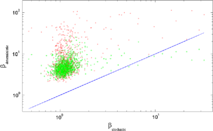
Figure 1: “$\times$,” “$+$” and the blue line correspond respectively to “$(\beta_{\mathrm{stochastic}},\beta_{\mathrm{uniform}})$,” “$(\beta_{\mathrm{stochastic}},\beta_{\mathrm{fractional}})$” and the identity function.

We define $\beta_{\mathrm{stochastic}}(\omega)$, $\beta_{\mathrm{uniform}}(\omega)$, $\beta_{\mathrm{fractional}}(\omega)$ where we compute$\beta_{\cdot}(\omega):=\frac{{N^{n}_{T}}\langle Z^{n}\rangle_{T}}{(\int_{0}^{T}\operatorname{Tr}(X_{t})\,\mathrm{d}t)^{2}}(\omega)$ according to each of these three strategies: in view of Theorem 3.2, this ratio is asymptotically greater than 1 and adimensional; moreover, the closer to 1 the ratio, the better the strategy.

Results. Figure 1 displays, for each $\omega$, the couples

$$\bigl{(}\beta_{\mathrm{stochastic}}(\omega),\beta_{\mathrm{uniform}}(\omega)\bigr{)}\quad\mbox{and}\quad\bigl{(}\beta_{\mathrm{stochastic}}(\omega),\beta_{\mathrm{fractional}}(\omega)\bigr{)}.$$

Most of the times, the points are above the diagonal, showing that the $\mu$-optimal strategy lessens the quadratic variation $\omega$-wise (remind that the strategies have got the same number of discrete times ${N^{n}_{T}}$), compared to the quadratic variation worked out over the deterministic time mesh. In addition, $\beta_{\mathrm{stochastic}}$ is concentrated around $1$, which means a convergence of ${N^{n}_{T}}\langle Z^{n}\rangle_{T}$ toward the lower bound $(\int_{0}^{T}\operatorname{Tr}(X_{t})\,\mathrm{d}t)^{2}$.

Figure 2 displays $\langle Z^{n}\rangle_{T}$ as a function of ${N^{n}_{T}}$ for the three strategies and for different $\omega$: here again, we observe that the $\mu$-optimal strategy outperforms deterministic strategies.

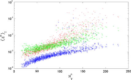
Figure 2: “$\times$,” “$+$” and correspond respectively to “$\langle Z^{n}\rangle_{T,\mathrm{uniform}}$,” “$\langle Z^{n}\rangle_{T,\mathrm{fractional}}$” and “$\langle Z^{n}\rangle_{T,\mathrm{stochastic}}$.”

Appendix

.3 Proof of Proposition 2.1

Let us prove (i), assuming only (A_S). For $p=0$, this is trivial.

Now consider the case $p>0$. Since $\sigma_{t}$ is nonzero for any $t$ and continuous, $C_{E}:=\inf_{t\in[0,T]}(\sum_{j=1}^{d}e_{j}\cdot\sigma_{t}\sigma_{t}^{*}e_{j})>0$ a.s., where $e_{j}$ is the $j$th element of the canonical basis in $\mathbb{R}^{d}$. Therefore, a.s. for any $0\leq s\leq t\leq T$ we have

$$0 \leq t-s\leq C_{E}^{-1}\int_{s}^{t}\Biggl{(}\sum_{j=1}^{d}e_{j}\cdot\sigma_{r}\sigma_{r}^{*}e_{j}\Biggr{)}\,\mathrm{d}r=C_{E}^{-1}\sum_{j=1}^{d}\bigl{[}\bigl{\langle}S^{j}\bigr{\rangle}_{t}-\bigl{\langle}S^{j}\bigr{\rangle}_{s}\bigr{]}$$

$$= C_{E}^{-1}\sum_{j=1}^{d}\biggl{[}\bigl{(}S^{j}_{t}-S^{j}_{s}\bigr{)}^{2}-2\int_{s}^{t}\bigl{(}S^{j}_{r}-S^{j}_{s}\bigr{)}\,\mathrm{d}S^{j}_{r}\biggr{]},$$

applying the Itô formula at the last equality. Take $s=\tau^{n}_{i-1}$, $t=\tau^{n}_{i}$ and use (A_S)

$$\Delta\tau^{n}_{i} \leq C_{E}^{-1}\Biggl{(}C_{0}\varepsilon_{n}^{2}+2\sum_{j=1}^{d}\biggl{|}\int_{\tau^{n}_{i-1}}^{\tau^{n}_{i}}\Delta S^{j}_{r}\,\mathrm{d}S^{j}_{r}\biggr{|}\Biggr{)}$$

$$\leq C_{E}^{-1}\Biggl{(}C_{0}\varepsilon_{n}^{2}+4\sum_{j=1}^{d}\sup_{0\leq t\leq T}\biggl{|}\int_{0}^{t}\Delta S^{j}_{r}\,\mathrm{d}S^{j}_{r}\biggr{|}\Biggr{)}.$$

Now for $j=1,\ldots,d$, set $M^{j,n}_{t}:=\varepsilon_{n}^{2/p-1}\int_{0}^{t}\Delta S^{j}_{r}\,\mathrm{d}S^{j}_{r}$ (recalling that $p>0$). Then

$$\sum_{n\geq 0}\bigl{\langle}M^{j,n}\bigr{\rangle}_{T}^{p/2}=\sum_{n\geq 0}\varepsilon_{n}^{2-p}\biggl{(}\int_{0}^{T}\bigl{|}\Delta S^{j}_{t}\bigr{|}^{2}\,\mathrm{d}\bigl{\langle}S^{j}\bigr{\rangle}_{t}\biggr{)}^{p/2}\leq C_{0}\sum_{n\geq 0}\varepsilon_{n}^{2}<+\infty\qquad\mbox{a.s.}$$

Thus owing to Corollary 2.1 the terms $(\sup_{0\leq t\leq T}|M^{j,n}_{t}|^{p})_{n\geq 0}$ define an a.s. convergent series. Combining this with (.3), we finally derive

$$\sum_{n\geq 0}\Bigl{[}\varepsilon_{n}^{2/p-1}\sup_{1\leq i\leq{N^{n}_{T}}}\bigl{|}\Delta\tau^{n}_{i}\bigr{|}\Bigr{]}^{p}$$

$$\qquad\leq C_{0}\Biggl{(}\sum_{n\geq 0}\bigl{[}\varepsilon_{n}^{2/p-1}\varepsilon_{n}^{2}\bigr{]}^{p}+\sum_{j=1}^{d}\sum_{n\geq 0}\sup_{0\leq t\leq T}\bigl{|}M^{j,n}_{t}\bigr{|}^{p}\Biggr{)}<+\infty\qquad\mbox{a.s.}$$

It remains to justify (ii). For $p=0$, the result directly follows from (A_N) and the inequality (6). Now take $p>0$, and set

$$U_{t}^{n} := {\varepsilon_{n}^{-2(p-1)+2\rho_{N}}}\sum_{\tau_{i-1}^{n}<t}\Biggl{|}\sum_{j=1}^{d}\Delta\bigl{\langle}S^{j}\bigr{\rangle}_{\tau^{n}_{i}\wedge t}\Biggr{|}^{p},$$

$$V_{t}^{n} := {\varepsilon_{n}^{-2(p-1)+2\rho_{N}}}\sum_{\tau_{i-1}^{n}<t}\ \sup_{s\in(\tau^{n}_{i-1},\tau^{n}_{i}\wedge t]}|\Delta S_{s}|^{2p}.$$

If $\sum_{n\geq 0}U_{T}^{n}\stackrel{{\scriptstyle a.s.}}{{\longrightarrow}}$, (.3) immediately yields that $\sum_{n\geq 0}{\varepsilon_{n}^{-2(p-1)+2\rho_{N}}}\times\break\sum_{\tau_{i-1}^{n}<T}(\Delta\tau^{n}_{i})^{p}\stackrel{{\scriptstyle a.s.}}{{\longrightarrow}}$. Thus, it is sufficient to show $\sum_{n\geq 0}U_{t}^{n}\stackrel{{\scriptstyle a.s.}}{{\longrightarrow}}$, for any $t\in[0,T]$, and this is achieved by an application of Lemma 2.2. The sequences of processes $(U^{n})_{n\geq 0}$ and $(V^{n})_{n\geq 0}$ are in $\mathcal{C}_{0}^{+}$. Then $V^{n}$ is nondecreasing, and using (A_S)–(A_N)

$$\sum_{n\geq 0}V_{T}^{n}\leq C_{0}\sum_{n\geq 0}{\varepsilon_{n}^{-2(p-1)+2\rho_{N}}}\varepsilon_{n}^{2p}{N^{n}_{T}}\leq C_{0}\sum_{n\geq 0}\varepsilon_{n}^{2}<+\infty\qquad\mbox{a.s.}$$

Then we deduce that items (i^′) and (ii^′) of Lemma 2.2 are fulfilled. It remains to check the relation of domination [item (iii^′)]. Let $k\in{\mathbb{N}}$. On the set $\{\tau^{n}_{i-1}<t\wedge\theta_{k}\}$, from the multidimensional BDG inequality in a conditional version, we have

$$\mathbb{E}\Biggl{(}\Biggl{|}\sum_{j=1}^{d}\Delta\bigl{\langle}S^{j}\bigr{\rangle}_{\tau^{n}_{i}\wedge t\wedge\theta_{k}}\Biggr{|}^{p}\Big{|}\mathcal{F}_{\tau^{n}_{i-1}}\Biggr{)}\leq c_{p}\mathbb{E}\Bigl{(}\sup_{\tau^{n}_{i-1}<s\leq\tau^{n}_{i}\wedge t\wedge\theta_{k}}|\Delta S_{s}|^{2p}\big{|}\mathcal{F}_{\tau^{n}_{i-1}}\Bigr{)}.$$ (29)

Then, it follows

$$\mathbb{E}\bigl{[}U_{t\wedge\theta_{k}}^{n}\bigr{]} = {\varepsilon_{n}^{-2(p-1)+2\rho_{N}}}\sum_{i=1}^{+\infty}\mathbb{E}\Biggl{(}1_{\tau^{n}_{i-1}<t\wedge\theta_{k}}\mathbb{E}\Biggl{[}\Biggl{|}\sum_{j=1}^{d}\Delta\langle S\rangle_{\tau^{n}_{i}\wedge t\wedge\theta_{k}}\Biggr{|}^{p}\Big{|}\mathcal{F}_{\tau^{n}_{i-1}}\Biggr{]}\Biggr{)}$$

$$\leq c_{p}\mathbb{E}\bigl{[}V_{t\wedge\theta_{k}}^{n}\bigr{]}.$$

The proof is complete.

.4 Proof of Proposition 2.2

Let $p>0$. Let $\delta$ be the parameter standing for $\frac{1}{2}$ under (A_S) and $1$ under (A_S)–(A_N). Set

$$U_{t}^{n} := {\varepsilon_{n}^{-2\delta(({p(\theta+1)}/2)-2(1-\delta))+2+2\rho_{N}(2\delta-1)}}\sum_{\tau_{i-1}^{n}<t}\sup_{\tau^{n}_{i-1}\leq s\leq\tau_{i}^{n}\wedge t}\bigl{|}\Delta M^{n}_{t}\bigr{|}^{p},$$

$$V_{t}^{n} := {\varepsilon_{n}^{-2\delta((p(\theta+1)/2)-2(1-\delta))+2+2\rho_{N}(2\delta-1)}}\sum_{\tau_{i-1}^{n}<t}\biggl{|}\int_{\tau^{n}_{i-1}}^{\tau^{n}_{i}\wedge t}\alpha^{n}_{r}\,\mathrm{d}r\biggr{|}^{p/2}.$$

Observe that the announced result reads as $\sum_{n\geq 0}U^{n}_{T}\stackrel{{\scriptstyle a.s.}}{{\longrightarrow}}$. To prove this convergence, it is enough to establish that $\sum_{n\geq 0}V^{n}_{T}\stackrel{{\scriptstyle a.s.}}{{\longrightarrow}}$. Indeed, following the arguments of the proof of Proposition 2.1(ii), we can apply Lemma 2.2 since $(U^{n})_{n\geq 0}$ and $(V^{n})_{n\geq 0}$ are two sequences of continuous adapted processes and: [(ii^′)]

$V^{n}$ is nondecreasing on $[0,T]$ a.s.;

the domination is satisfied thanks to the BDG inequalities, similarly to (29). Now to prove (ii^′), that is, $\sum_{n\geq 0}V^{n}_{T}\stackrel{{\scriptstyle a.s.}}{{\longrightarrow}}$, write

$$\sum_{n\geq 0}V_{T}^{n} \leq \sum_{n\geq 0}{\varepsilon_{n}^{-2\delta(({p(\theta+1)}/2)-2(1-\delta))+2+2\rho_{N}(2\delta-1)}}$$

$$\hskip 15.0pt{}\times\sum_{\tau_{i-1}^{n}<T}\bigl{|}C_{0}\bigl{(}\varepsilon_{n}^{2\theta}+\bigl{(}\Delta\tau^{n}_{i}\bigr{)}^{\theta}\bigr{)}\Delta\tau^{n}_{i}\bigr{|}^{p/2}\qquad\mbox{a.s.}$$

First, consider the case (A_S) and set $D_{n}^{(q)}:=\sup_{1\leq i\leq N^{n}_{T}}(\Delta\tau^{n}_{i})^{q}$ for $q\geq 0$: Proposition 2.1(i) yields ${\mathcal{D}}^{(q)}:=\sum_{n\geq 0}\varepsilon_{n}^{-(q-2)}D_{n}^{(q)}<+\infty$ a.s. Using $p\geq 2$, it readily follows that

$$\sum_{n\geq 0}V_{T}^{n} \leq \sum_{n\geq 0}\varepsilon_{n}^{{-(p(\theta+1)/2-3)}}C_{0}^{p/2}\sum_{\tau_{i-1}^{n}<T}\bigl{(}\varepsilon_{n}^{2\theta}+\bigl{(}\Delta\tau^{n}_{i}\bigr{)}^{\theta}\bigr{)}^{p/2}\bigl{(}\Delta\tau^{n}_{i}\bigr{)}^{p/2-1}\Delta\tau^{n}_{i}$$

$$\leq \sum_{n\geq 0}\varepsilon_{n}^{{-(p(\theta+1)/2-3)}}C_{0}^{p/2}2^{p/2-1}T\bigl{(}\varepsilon_{n}^{p\theta}D_{n}^{(p/2-1)}+D_{n}^{((\theta+1)p/2-1)}\bigr{)}$$

$$\leq C_{0}^{p/2}2^{p/2-1}T\Bigl{(}\Bigl{(}\sup_{n\geq 0}\varepsilon_{n}\Bigr{)}^{p\theta/2}{\mathcal{D}}^{(p/2-1)}+{\mathcal{D}}^{((\theta+1)p/2-1)}\Bigr{)}<+\infty\qquad\mbox{a.s.}$$

Second for the case (A_S)–(A_N), setting $D_{n}^{(q)}:=\sum_{\tau_{i-1}^{n}<T}(\Delta\tau^{n}_{i})^{q}$ for $q\geq 0$, we have ${\mathcal{D}}^{(q)}:=\sum_{n\geq 0}{\varepsilon_{n}^{-2(q-1)+2\rho_{N}}}D_{n}^{(q)}<+\infty$ a.s., thanks to Proposition 2.1(ii). Then we easily deduce (for any $p>0$)

$$\sum_{n\geq 0}V_{T}^{n} \leq C_{0}^{p/2}2^{(p/2-1)_{+}}\sum_{n\geq 0}{\varepsilon_{n}^{-2(p(\theta+1)/2-1)+2\rho_{N}}}$$

$$\hskip 80.0pt{}\times\sum_{\tau_{i-1}^{n}<T}\bigl{(}\varepsilon_{n}^{p\theta}\bigl{(}\Delta\tau^{n}_{i}\bigr{)}^{p/2}+\bigl{(}\Delta\tau^{n}_{i}\bigr{)}^{(\theta+1)p/2}\bigr{)}$$

$$= C_{0}^{p/2}2^{(p/2-1)_{+}}\bigl{(}{\mathcal{D}}^{(p/2)}+{\mathcal{D}}^{((\theta+1)p/2)}\bigr{)}<+\infty\qquad\mbox{a.s.}$$

.5 Proof of Proposition 2.4

It is standard to check that ${\mathcal{T}}^{n}$ is a sequence of increasing stopping times; we skip details. Let us justify that the size of ${\mathcal{T}}^{n}$ is a.s. finite, for any $n\geq 0$. For a given $n\geq 0$, define the event ${\mathcal{N}}^{n}:=\{{N^{n}_{T}}=+\infty\}$. For $\omega\in{\mathcal{N}}^{n}$, the infinite sequence $(\tau^{n}_{i}{(\omega)})_{i\geq 0}$ converges, because increasing and bounded by $T$. Thus, on ${\mathcal{N}}^{n}\cap E_{S}$ with $E_{S}=\{(S_{t})_{0\leq t\leq T}$ continuous and $\sup_{0\leq t<T}\lambda_{\mathrm{max}}(H_{t})<+\infty\}$, we have

$$0<\varepsilon_{n} = (S_{\tau^{n}_{i}}-S_{\tau^{n}_{i-1}})^{*}H_{\tau^{n}_{i-1}}(S_{\tau^{n}_{i}}-S_{\tau^{n}_{i-1}})$$

$$\leq \sup_{0\leq t<T}\lambda_{\mathrm{max}}(H_{t})|S_{\tau^{n}_{i}}-S_{\tau^{n}_{i-1}}|^{2}\mathop{\rightarrow}_{i\rightarrow+\infty}0,$$

which is impossible. Thus, ${\mathcal{N}}^{n}\subset E^{c}_{S}$ and $\mathbb{P}({\mathcal{N}}^{n})=0$ since $S$ is a.s. continuous and $\sup_{0\leq t<T}\lambda_{\mathrm{max}}(H_{t})$ is a.s. finite.

Besides, we have $C_{H}:=\inf_{0\leq t<T}\lambda_{\mathrm{min}}(H_{t})>0$ a.s., and we immediately get

$$\varepsilon_{n}^{-2}\sup_{1\leq i\leq N^{n}_{T}}\sup_{t\in(\tau^{n}_{i-1},\tau^{n}_{i}]}|\Delta S_{t}|^{2}\leq C_{H}^{-1}\varepsilon_{n}^{-2}\sup_{1\leq i\leq N^{n}_{T}}\sup_{t\in(\tau^{n}_{i-1},\tau^{n}_{i}]}\bigl{(}\Delta S_{t}^{*}H_{\tau^{n}_{i-1}}\Delta S_{t}\bigr{)}\leq C_{H}^{-1},$$

which validates the assumption (A_S).

Then, writing ${N^{n}_{T}}=1+\sum_{1\leq i\leq{N^{n}_{T}}-1}1$, we point out (for $n$ large enough so that $\varepsilon_{n}\leq 1$)

$$\varepsilon_{n}^{2\rho_{N}}{N^{n}_{T}} \leq \varepsilon_{n}^{2}{N^{n}_{T}}$$

$$\leq \varepsilon_{n}^{2}+\sum_{1\leq i\leq{N^{n}_{T}}-1}\Delta S_{\tau^{n}_{i}}^{*}H_{\tau^{n}_{i-1}}\Delta S_{\tau^{n}_{i}}\leq\varepsilon_{n}^{2}+\sum_{\tau_{i-1}^{n}<T}\Delta S_{\tau^{n}_{i}}^{*}H_{\tau^{n}_{i-1}}\Delta S_{\tau^{n}_{i}};$$

using moreover from Proposition 2.3, we know that under the assumption (A_S) only,

$$\sum_{\tau_{i-1}^{n}<T}\Delta S_{\tau^{n}_{i}}^{*}H_{\tau^{n}_{i-1}}\Delta S_{\tau^{n}_{i}}\stackrel{{\scriptstyle a.s.}}{{\longrightarrow}}\int_{0}^{T}\operatorname{Tr}\bigl{(}H_{t}\,\mathrm{d}\langle S\rangle_{t}\bigr{)}<+\infty.$$

This validates the assumption (A_N).

Remark .1.

The structure of hitting times of ellipsoids with size $\varepsilon_{n}$ has a specific feature compared to general admissible strategies: the assumption (A_S) entails the assumption (A_N).

.6 Proof of Lemma 3.1

We split the proof into several steps. Let

$$h\dvtx\cases{\mathbb{R}^{d}\times\mathbb{R}_{+}\rightarrow\mathbb{R},\vspace*{2pt}\cr\displaystyle(\lambda,y)\mapsto(4+d)y-\sum_{i=1}^{d}\sqrt{y^{2}+4\lambda_{i}^{2}}.}$$

Assume for a while that:

1. [$(\star)$]

2. 1. [(a)]

   2. for any $\lambda\in\mathbb{R}^{d}$, there exists a unique nonnegative root $y_{\lambda}$ satisfying $h(\lambda,y_{\lambda})=0$;

   3. $y_{0}=0$; $\lambda\neq 0\Rightarrow y_{\lambda}>0$;

   4. the mapping $\lambda\mapsto y_{\lambda}$ is continuous.

Necessary conditions on the spectrum of $x(c)$. Let $\operatorname{Diag}$ denote the set of $d\times d$ diagonal matrices. Take $c\in\mathcal{S}^{d}(\mathbb{R})$ and let $x(c)\in\mathcal{S}^{d}_{+}(\mathbb{R})$ be a solution (whenever it exists) to (12). Then by the spectral theorem, $x(c)$ is diagonalizable: there exists an orthogonal matrix $p_{x(c)}$ such that $p_{x(c)}^{*}x(c)p_{x(c)}\in\operatorname{Diag}$. Equation (12) is stable by unitary transformation

$$2\operatorname{Tr}\bigl{(}p_{x(c)}^{*}x(c)p_{x(c)}\bigr{)}p_{x(c)}^{*}x(c)p_{x(c)}+4\bigl{(}p_{x(c)}^{*}x(c)p_{x(c)}\bigr{)}^{2}$$

(30)

$$\qquad=p_{x(c)}^{*}c^{2}p_{x(c)}\in\operatorname{Diag}.$$

The diagonal elements of $p_{x(c)}^{*}c^{2}p_{x(c)}$ must be the eigenvalues of $c^{2}$, that is the square of the eigenvalues of $c$ [which is in $\mathcal{S}^{d}(\mathbb{R})$]. Identifying the diagonal elements from (.6) gives a relation between the spectra of $c$ and $x(c)$,

$$2\operatorname{Tr}\bigl{(}x(c)\bigr{)}\lambda_{i}\bigl{(}x(c)\bigr{)}+4\lambda_{i}\bigl{(}x(c)\bigr{)}^{2}=\lambda_{i}(c)^{2},\qquad 1\leq i\leq d.$$

Thus, the nonnegative eigenvalues of $x(c)$ must satisfy $\lambda_{i}(x(c))=\break(-\operatorname{Tr}(x(c))+\sqrt{\operatorname{Tr}(x(c))^{2}+4\lambda_{i}(c)^{2}})/4$. By summing over $i=1,\ldots,d$, we obtain an implicit equation for $\operatorname{Tr}(x(c))$, which is $h(\lambda(c),\operatorname{Tr}(x(c)))=0$. By $(\star)$, there is a unique solution and

$$\operatorname{Tr}\bigl{(}x(c)\bigr{)}=y_{\lambda(c)}.$$ (31)

Thus, we have proved that the eigenvalues of $x(c)$ must be

$$\lambda_{i}\bigl{(}x(c)\bigr{)}=\frac{-y_{\lambda(c)}+\sqrt{y_{\lambda(c)}^{2}+4\lambda_{i}(c)^{2}}}{4}.$$ (32)

Existence/uniqueness of solution to (12). Take $c\in\mathcal{S}^{d}(\mathbb{R})$. Starting from (12), owing to (31) $x(c)$ must solve

$$\bigl{(}2x(c)+\tfrac{1}{2}y_{\lambda(c)}I_{d}\bigr{)}^{2}=\tfrac{1}{4}y^{2}_{\lambda(c)}I_{d}+c^{2}.$$

The matrix $c^{2}+\frac{1}{4}y^{2}_{\lambda(c)}I_{d}$ is symmetric nonnegative-definite, and thus it has a unique square-root (symmetric nonnegative-definite matrix) HJ90 , Theorem 7.2.6, page 405, and we obtain

$$x(c):=-\frac{y_{\lambda(c)}}{4}I_{d}+\frac{1}{2}\biggl{(}\frac{y_{\lambda(c)}^{2}}{4}I_{d}+c^{2}\biggr{)}^{1/2}.$$ (33)

The uniqueness is proved. It is now easy to check that $x(c)$ given in (33) solves (12), using the implicit equation satisfied by $\operatorname{Tr}(x(c))$. Last, $\lambda_{\mathrm{min}}(c^{2})>0$ if and only if $\lambda_{\mathrm{min}}(x(c))>0$ [owing to (32)].

Continuity. From Hoffman and Wielandt’s theorem HJ90 , page 368, the function $c\mapsto\lambda(c)$ is continuous on $\mathcal{S}^{d}(\mathbb{R})$ into $\mathbb{R}^{d}$. Hence, combined with $(\star)(c)$, we obtain the continuity of $c\mapsto y_{\lambda(c)}$ on $\mathcal{S}^{d}(\mathbb{R})$ into $\mathbb{R}$.

Then, the continuity of $x(\cdot)$ at $c_{0}=0$ easily follows since as $c\rightarrow 0$, $y_{\lambda(c)}\rightarrow y_{0}=0$ and $\lambda(x(c))\rightarrow 0$ [using (32)]: thus $x(c)\rightarrow 0=x_{0}$. For $c_{0}\neq 0$, we invoke the property that $c\mapsto c^{1/2}$ is locally lipschitz (and even analytic) on $\mathcal{S}^{d}_{++}(\mathbb{R})$ into $\mathcal{S}^{d}_{++}(\mathbb{R})$ (SV97 , Lemma 5.2.1 page 131): we use this with $\frac{y_{\lambda(c)}^{2}}{4}I_{d}+c^{2}\in\mathcal{S}^{d}_{++}(\mathbb{R})$ for $c$ close enough to $c_{0}$ (using $y_{\lambda(c)}>0$ for $c\neq 0$). In view of (33), the continuity of $x(\cdot)$ at $c_{0}\neq 0$ follows.

Proof of $(\star)$. $h$ is continuous on $\mathbb{R}^{d}\times[0,\infty[$ into $\mathbb{R}$. Moreover:

• $h(\lambda,0)=-2\sum_{i=1}^{d}|\lambda_{i}|\leq 0$ and $\lim_{y\rightarrow+\infty}h(\lambda,y)=+\infty$;

• $h$ is continuously differentiable on $\mathbb{R}^{d}\times\,]0,\infty[$;

• $D_{y}h(\lambda,y)=4+d-\sum_{1\leq j\leq d}\frac{y}{\sqrt{y^{2}+4\lambda_{i}^{2}}}\geq 4$, implying that $y\mapsto{h}(\lambda,y)$ is (strictly) increasing.

Then, there is a unique $y_{\lambda}\in\mathbb{R}_{+}$ such that $h(\lambda,y_{\lambda})=0$. We point out at first glance, $\lambda\neq 0\Leftrightarrow y_{\lambda}>0.$ The continuity of $y_{\cdot}$ is proved on $\mathbb{R}_{*}^{d}$ on the one hand, and at $0$ on the other hand.

• On $\mathbb{R}_{*}^{d}\times\,]0,+\infty[\dvtx D_{y}h(\lambda,y)$ exists and is nonzero: then by the implicit function theorem, there exists an open set $U\subset\mathbb{R}^{d}_{*}$ containing $\lambda$ and an open set $V\subset]0,+\infty[$ containing $y_{\lambda}$ such that $y$ is continuously differentiable from $U$ to $V$. This proves the continuously differentiability of $y_{\cdot}$ in $\mathbb{R}^{d}_{*}$.

• At $\lambda=0\dvtx h((|\lambda|)_{1\leq i\leq d},y)\leq h(\lambda,y)$ and $y\geq\frac{d|\lambda|}{\sqrt{4+2d}}\Leftrightarrow h((|\lambda|)_{1\leq i\leq d},y)\geq 0$. It implies $0\leq y_{\lambda}\leq\frac{d|\lambda|}{\sqrt{4+2d}}$ and $\lim_{|\lambda|\rightarrow 0}y_{\lambda}=0$.

That completes the continuity of $\lambda\mapsto y_{\lambda}$ on $\mathbb{R}^{d}$ and by the previous discussion, the proof of the lemma.∎

.7 Proof of Lemma 3.2

We have $\langle R^{n}\rangle_{T}=\int_{0}^{T}|\sigma_{t}^{*}(D_{x}u_{t}-D_{x}u_{\varphi(t)}-D^{2}_{xx}u_{\varphi(t)}\Delta S_{t})|^{2}\,\mathrm{d}t$: to prove the result, we aim at performing a Taylor expansion using (A_u), that is, derivatives of $u$ are a.s. finite in a small tube around $(t,S_{t},Y_{t})_{0\leq t\leq T}$. Because of this local assumption, a careful treatment is required, which we now detail. In view of (A_u), there exists $\Omega_{\mathcal{D}}$ such that $\mathbb{P}(\Omega_{\mathcal{D}})=1$ and for every $\omega\in\Omega_{\mathcal{D}}$ there is $\delta(\omega)>0$ such that

$$|{\mathcal{A}}u|_{\delta}(\omega):=\sup_{0\leq t<T}\sup_{|x-S_{t}(\omega)|\leq\delta(\omega),|y-Y_{t}(\omega)|\leq\delta(\omega)}\bigl{|}\mathcal{A}u(t,x,y)\bigr{|}<+\infty$$

for any $\mathcal{A}\in\mathcal{D}:=\{D^{2}_{x_{j}x_{k}},D^{3}_{x_{j}x_{k}x_{l}},D^{2}_{tx_{j}},D^{2}_{x_{j}y_{m}}\dvtx 1\leq j,k,l\leq d,1\leq m\leq d^{\prime}\}$.

Since $\sup_{1\leq i\leq N^{n}_{T}}\Delta\tau^{n}_{i}\stackrel{{\scriptstyle a.s.}}{{\longrightarrow}}0$ and $(S_{t},Y_{t})_{0\leq t\leq T}$ are a.s. continuous on the compact interval $[0,T]$, there exists $\Omega_{\mathcal{C}}$ with $\mathbb{P}(\Omega_{\mathcal{C}})=1$ such that for every $\omega\in\Omega_{\mathcal{C}}$, there is $p(\omega)\in\mathbb{N}$ such that $\forall n\geq p(\omega)$,

$$\Bigl{(}\sup_{0\leq s,t\leq T,|t-s|\leq\sup_{1\leq i\leq N^{n}_{T}}\Delta\tau^{n}_{i}}|S_{t}-S_{s}|\lor|Y_{t}-Y_{s}|\Bigr{)}(\omega)\leq\delta(\omega).$$

Hence for $\omega\in\Omega_{\mathcal{D}}\cap\Omega_{\mathcal{C}}$, let $n\geq p(\omega)$, $i\in\{1,\ldots,{N^{n}_{T}}\}$ and $t\in[\tau^{n}_{i-1},\tau^{n}_{i}]$, and write

$$D_{x}u(t,S_{t},Y_{t})-D_{x}u\bigl{(}\tau^{n}_{i-1},S_{\tau^{n}_{i-1}},Y_{\tau^{n}_{i-1}}\bigr{)}-D^{2}_{xx}u\bigl{(}\tau^{n}_{i-1},S_{\tau^{n}_{i-1}},Y_{\tau^{n}_{i-1}}\bigr{)}\Delta S_{t}$$

$$\qquad=\bigl{[}D_{x}u(t,S_{t},Y_{t})-D_{x}u\bigl{(}\tau^{n}_{i-1},S_{t},Y_{t}\bigr{)}\bigr{]}$$

$$\qquad\quad{}+\bigl{[}D_{x}u\bigl{(}\tau^{n}_{i-1},S_{t},Y_{t}\bigr{)}-D_{x}u\bigl{(}\tau^{n}_{i-1},S_{t},Y_{\tau^{n}_{i-1}}\bigr{)}\bigr{]}$$

$$\qquad\quad{}+\bigl{[}D_{x}u\bigl{(}\tau^{n}_{i-1},S_{t},Y_{\tau^{n}_{i-1}}\bigr{)}-D_{x}u\bigl{(}\tau^{n}_{i-1},S_{\tau^{n}_{i-1}},Y_{\tau^{n}_{i-1}}\bigr{)}$$

$$\hskip 83.0pt\qquad\quad{}-D^{2}_{xx}u\bigl{(}\tau^{n}_{i-1},S_{\tau^{n}_{i-1}},Y_{\tau^{n}_{i-1}}\bigr{)}\Delta S_{t}\bigr{]}.$$

Now apply Taylor’s theorem to the terms above, by observing that the involved derivatives of $u$ are locally bounded by the (a.s. finite) random variable $C_{u}:=\max_{\mathcal{A}\in\mathcal{D}}|{\mathcal{A}}u|_{\delta}$,

$$\bigl{|}D_{x}u(t,S_{t},Y_{t})-D_{x}u\bigl{(}\tau^{n}_{i-1},S_{\tau^{n}_{i-1}},Y_{\tau^{n}_{i-1}}\bigr{)}-D^{2}_{xx}u\bigl{(}\tau^{n}_{i-1},S_{\tau^{n}_{i-1}},Y_{\tau^{n}_{i-1}}\bigr{)}\Delta S_{t}\bigr{|}$$

$$\qquad\leq\sqrt{d}C_{u}\biggl{(}\bigl{(}t-\tau^{n}_{i}\bigr{)}+\sqrt{d^{\prime}}|Y_{t}-Y_{\tau^{n}_{i-1}}|+\frac{d}{2}|\Delta S_{t}|^{2}\biggr{)}.$$

Plugging this estimate into $\langle R^{n}\rangle_{T}$ and using that $Y$ is nondecreasing, we derive that a.s. for $n$ large enough,

$${\varepsilon_{n}^{2-4\rho_{N}}}\bigl{\langle}R^{n}\bigr{\rangle}_{T}$$

$$\qquad\leq 3dC_{u}^{2}\sup_{0\leq t\leq T}|\sigma_{t}|^{2}{\varepsilon_{n}^{2-4\rho_{N}}}\sum_{\tau_{i-1}^{n}<T}\biggl{(}\bigl{(}\Delta\tau^{n}_{i}\bigr{)}^{3}+d^{\prime}|\Delta Y_{\tau^{n}_{i}}|^{2}\Delta\tau^{n}_{i}$$

$$\hskip 141.0pt\qquad\quad{}+\frac{d^{2}}{4}\Delta\tau^{n}_{i}\sup_{\tau^{n}_{i-1}\leq t\leq\tau_{i}^{n}}|\Delta S_{t}|^{4}\biggr{)}.$$

To prove the a.s. convergence of the upper bound to 0, we separately analyze each of the three contributions:

• $\varepsilon_{n}^{2-4\rho_{N}}\sum_{\tau_{i-1}^{n}<T}(\Delta\tau^{n}_{i})^{3}\leq\varepsilon_{n}^{2-4\rho_{N}}{N^{n}_{T}}\sup_{1\leq i\leq N^{n}_{T}}(\Delta\tau^{n}_{i})^{3}\leq C_{0}\varepsilon_{n}^{4-3\rho_{N}}\stackrel{{\scriptstyle a.s.}}{{\longrightarrow}}0$ by Corollary 2.2(ii) with $\rho=\frac{4}{3}-\rho_{N}>0$; see (A_N).

• Combining (A_Y) and Corollary 2.2(ii) with $\rho=\frac{\rho_{Y}}{2}-2(\rho_{N}-1)>0$, we easily obtain

  $${\varepsilon_{n}^{2-4\rho_{N}}}\sum_{\tau_{i-1}^{n}<T}|\Delta Y_{\tau^{n}_{i}}|^{2}\Delta\tau^{n}_{i} \leq \sum_{j=1}^{d^{\prime}}\bigl{(}Y^{j}_{T}-Y^{j}_{0}\bigr{)}{\varepsilon_{n}^{2-4\rho_{N}}}\sup_{1\leq i\leq N^{n}_{T}}\bigl{|}\Delta Y^{j}_{\tau^{n}_{i}}\bigr{|}\sup_{1\leq i\leq N^{n}_{T}}\Delta\tau^{n}_{i}$$

  $$\leq \sqrt{d^{\prime}}|Y_{T}-Y_{0}|C_{0}{\varepsilon_{n}^{2-4\rho_{N}}}\varepsilon_{n}^{\rho_{Y}}\varepsilon_{n}^{2-\rho}$$

  $$\leq C_{0}{\varepsilon_{n}^{\rho_{Y}/2-2(\rho_{N}-1)}}\stackrel{{\scriptstyle a.s.}}{{\longrightarrow}}0.$$

• Using (A_S), ${\varepsilon_{n}^{2-4\rho_{N}}}\sum_{\tau_{i-1}^{n}<T}\Delta\tau^{n}_{i}\sup_{\tau^{n}_{i-1}\leq t\leq\tau_{i}^{n}}|\Delta S_{t}|^{4}\leq C_{0}{\varepsilon_{n}^{6-4\rho_{N}}}T\stackrel{{\scriptstyle a.s.}}{{\longrightarrow}}0$ since $\rho_{N}<\frac{3}{2}$.

All these convergences lead to the results.

.8 Assumption (A_u)

We show that assumption (A_u) is satisfied in most usual situations, even if the payoff $g$ is not smooth. Actually, we have not been able to exhibit an example of $g$ for which (A_u) does not hold. The following discussion should convince the reader that finding a counter-example is far from being straightforward, but we conjecture that it is possible.

Vanilla option in Black–Scholes model. For pedagogic reasons, we start with the one-dimensional log-normal model $\,\mathrm{d}S_{t}=\sigma S_{t}\,\mathrm{d}B_{t}$ ($\sigma>0$). Consider first the Call option with strike $K>0$: for $t<T$ we have $D_{x}u(t,x)={\mathcal{N}}(\frac{\log(x/K)}{\sigma\sqrt{T-t}}+\frac{1}{2}\sigma\sqrt{T-t})\in[0,1]$ where ${\mathcal{N}}(\cdot)$ is the c.d.f. of the standard Gaussian law. The second derivative writes

$$D^{2}_{xx}u(t,x)=\frac{1}{\sigma x\sqrt{2\pi(T-t)}}\exp\biggl{(}-\frac{1}{2}\biggl{[}\frac{\log(x/K)}{\sigma\sqrt{T-t}}+\frac{1}{2}\sigma\sqrt{T-t}\biggr{]}^{2}\biggr{)};$$

thus bounding the exponential term by $1$, we have for any given $t_{0}<T$ $\lim_{\delta\rightarrow 0}\sup_{0\leq t\leq t_{0}}\sup_{|x-S_{t}|\leq\delta}|D^{2}_{xx}u(t,x)|\leq\frac{1}{\sigma\inf_{0\leq t\leq T}S_{t}\sqrt{2\pi(T-t_{0})}}<+\infty$.It shows that an a.s. finite bound on the second derivative is available provided that the time to maturity does not vanish. For the third derivative, this is similar: indeed using $\sup_{y\in\mathbb{R}}e^{y^{2}/4}|\partial_{y}(e^{-y^{2}/2})|=\sup_{y\in\mathbb{R}}|y|e^{-y^{2}/4}=\sqrt{2}e^{-1/2}\leq 1$, we deduce

$$\bigl{|}D^{3}_{xxx}u(t,x)\bigr{|}\leq\frac{1+\sigma\sqrt{T}}{x^{2}\sqrt{2\pi}\sigma^{2}(T-t)}\exp\biggl{(}-\frac{1}{4}\biggl{[}\frac{\log(x/K)}{\sigma\sqrt{T-t}}+\frac{1}{2}\sigma\sqrt{T-t}\biggr{]}^{2}\biggr{)},$$

and as before $\lim_{\delta\rightarrow 0}\sup_{0\leq t\leq t_{0}}\sup_{|x-S_{t}|\leq\delta}|D^{3}_{xxx}u(t,x)|<+\infty$ for any given $t_{0}<T$.

The next step consists in deriving a.s. upper bounds on derivatives for arbitrary small time to maturity. We take advantage of the property $\mathbb{P}(S_{T}\neq K)=1$, which implies (by a.s. continuity of $S$) that for $\mathbb{P}$-a.e. $\omega$ there exists $t_{0}(\omega)\in[0,T[$ such that $\inf_{t_{0}(\omega)\leq t\leq T}|S_{t}(\omega)-K|\geq|S_{T}(\omega)-K|/2:=2\delta_{0}(\omega)>0$. Then, for $t\in[t_{0}(\omega),T]$ and $\delta\leq\delta_{0}\land[2^{-1}\inf_{0\leq t\leq T}S_{t}]$, we have $\inf_{|x-S_{t}|\leq\delta}|\log(x/K)|\geq\inf_{u>0\dvtx|u-1|\geq\delta_{0}/K}|\log(u)|:=c(\omega)>0$ and$\inf_{|x-S_{t}|\leq\delta}x\geq S_{t}/2$: therefore using the inequality $-(\alpha+\beta)^{2}\leq-\frac{\alpha^{2}}{2}+\beta^{2}$, we obtain, for $t\in[t_{0}(\omega),T[$

$$\sup_{|x-S_{t}|\leq\delta}\bigl{|}D^{2}_{xx}u(t,x)\bigr{|}\leq\frac{2}{\sigma S_{t}\sqrt{2\pi(T-t)}}\exp\biggl{(}-\frac{c^{2}(\omega)}{4\sigma^{2}(T-t)}+\frac{1}{8}\sigma^{2}T\biggr{)}.$$

Observe that $c(\omega)>0$ implies that the above upper boundconverges to 0 as $t\rightarrow T$: thus, we have completed the proof of$\lim_{\delta\rightarrow 0}\sup_{0\leq t<T}\sup_{|x-S_{t}|\leq\delta}|D_{xx}^{2}u(t,x)|<+\infty$ a.s. For the third derivative, similarly we obtain for $t\in[t_{0}(\omega),T[$ and $\delta\leq\delta_{0}(\omega)\land[2^{-1}\inf_{0\leq t\leq T}S_{t}(\omega)]$

$$\sup_{|x-S_{t}|\leq\delta}\bigl{|}D^{3}_{xxx}u(t,x)\bigr{|}\leq\frac{4(1+\sigma\sqrt{T})}{S^{2}_{t}\sqrt{2\pi}\sigma^{2}(T-t)}\exp\biggl{(}-\frac{c^{2}(\omega)}{8\sigma^{2}(T-t)}+\frac{1}{16}\sigma^{2}T\biggr{)},$$

and we conclude as for the second derivative. To derive the property for $D^{2}_{tx}u$, we use the relation $D^{2}_{tx}u=-\frac{1}{2}\sigma^{2}x^{2}D^{3}_{xxx}u-\sigma^{2}xD^{2}_{xx}u$. Finally, (A_u) is proved for the call option (and thus for the put option).

The same argumentation can be applied for the digital call option which payoff is of the form $g(x)=\mathbf{1}_{x\geq K}$: indeed, the derivatives of $u$ blow up only at the discontinuity point $K$ which has null probability for the law of $S_{T}$. (A_u) holds for digital options.

Vanilla option in general local volatility model. The previous arguments are based on the explicit Black–Scholes formula for call and digital call options, but we can generalize them to more general models and payoffs and handle derivatives at any order. Denote by $X^{j}=\log(S^{j})$ ($1\leq j\leq d$) the log-asset price in a diffusion model, and assume that $\,\mathrm{d}X_{t}=b^{X}(t,X_{t})\,\mathrm{d}t+\sigma^{X}(t,X_{t})\,\mathrm{d}B_{t}$ for coefficients $b^{X}$ and $\sigma^{X}$ of class $\mathcal{C}_{b}^{\infty}([0,T]\times\mathbb{R}^{d})$ (bounded with bounded derivatives). The price function in the log-variables is then $v(t,x):=u(t,\exp(x^{1}),\ldots,\exp(x^{d}))=\mathbb{E}(g(S_{T})|S^{j}_{t}=\exp(x^{j}),1\leq j\leq d):=\break\mathbb{E}(G(X_{T})|X_{t}=x)$. We first consider the simple case of ${\mathcal{C}}^{\infty}$-payoff $G$ with exponentially bounded derivatives: for any $k\geq 0$, there is a constant $C^{G}_{k}\geq 0$ such that $|D^{k}_{x}G(x)|\leq C^{G}_{k}\exp(C^{G}_{k}|x|)$ for $x\in\mathbb{R}^{d}$. In this case, a direct differentiation of $\mathbb{E}(G(X_{T})|X_{t}=x)$ using the smooth flow $x\mapsto X_{T}^{t,x}$ kuni:84 shows the differentiability of $v$ w.r.t. the space variable with derivatives bounded on compact subsets of $[0,T]\times\mathbb{R}^{d}$; in addition the time smoothness is obtained using Itô’s formula; these arguments are standard and we skip details. (A_u) is proved for these smooth payoffs.

Now we tackle the case of discontinuous payoffs of the form $G(x)=\mathbf{1}_{x\in\mathcal{D}}\varphi(x)$ for a closed set $\mathcal{D}\subset\mathbb{R}^{d}$ and a $\mathcal{C}^{\infty}$-function $\varphi$ with exponentially bounded derivatives: observe that by combining the analysis for smooth payoffs and that for discontinuous ones will allow to cover a quite large class of $g$ satisfying (A_u) (such as call/put, digital call/put, exchange call, digital exchange call and so on). We assume that a uniform ellipticity assumption is satisfied: $\inf_{0\leq t\leq T,x\in\mathbb{R}^{d}}\inf_{|\xi|=1}\xi\cdot[\sigma^{X}(\sigma^{X})^{*}](t,x)\xi>0$. In this setting, $v(t,x)=\int_{\mathbb{R}^{d}}\mathbf{1}_{z\in\mathcal{D}}p(t,x,T,z)\varphi(z)\,\,\mathrm{d}z$ where $p$ is the transition density function of $X$, which is smooth and satisfies to Aronson-type estimates (frie:64 , Theorem 8, page 263): for any $i\geq 0$ and any differentiation index $\alpha$, there exists a constant $C_{i,\alpha}=C_{i,\alpha}(T,b^{X},\sigma^{X})>0$ such that

$$\bigl{|}D^{i,\alpha}_{tx}p(t,x,T,z)\bigr{|}\leq C_{i,\alpha}(T-t)^{-(d+2i+|\alpha|)/2}\exp\bigl{(}-|x-z|^{2}/\bigl{[}C_{i,\alpha}(T-t)\bigr{]}\bigr{)}$$

for any $0\leq t<T$, $x\in\mathbb{R}^{d}$, $z\in\mathbb{R}^{d}$. From the integral representation of $v$, it readily follows that

$$\bigl{|}D^{i,\alpha}_{tx}v(t,x)\bigr{|}$$

$$\qquad\leq C_{i,\alpha}(T-t)^{-(2i+|\alpha|)/2}\int_{\mathbb{R}^{d}}C^{\varphi}_{0}e^{C_{0}^{\varphi}|z|}(T-t)^{-d/2}e^{-|x-z|^{2}/[C_{i,\alpha}(T-t)]}\,\,\mathrm{d}z$$

$$\qquad\leq C_{i,\alpha}(T-t)^{-(2i+|\alpha|)/2}C^{\varphi}_{0}e^{C_{0}^{\varphi}|x|}\int_{\mathbb{R}^{d}}e^{C_{0}^{\varphi}\sqrt{T}|w|}e^{-|w|^{2}/C_{i,\alpha}}\,\mathrm{d}w,$$

which proves locally uniform bounds on derivatives provided that the time to maturity remains bounded away from 0. To handle the case $t\rightarrow T$, we additionally assume that the boundary $\partial\mathcal{D}$ of $\mathcal{D}$ is Lebesgue-negligible (thus including usual situations but excluding Cantor like sets; see dibe:02 , page 114): thus for $\mathbb{P}$-a.e. $\omega$, the distance to the boundary (a closed set) is positive, that is, $\delta_{0}(\omega):=\frac{1}{4}d(X_{T}(\omega),\partial\mathcal{D})>0$, and there exists $t_{0}(\omega)\in[0,T[$ such that $\inf_{t_{0}(\omega)\leq t\leq T}d(X_{t}(\omega),\partial\mathcal{D})\geq 3\delta_{0}(\omega)$ [we recall that the distance function $x\mapsto d(x,\partial\mathcal{D})$ is Lipschitz continuous]. Now, let $\omega$ be given as above; by the smooth version of the Urysohn lemma dieu:90:1 , page 90, Chapter IV, there exists a smooth function $\xi$ (depending on $\omega$) such that $\mathbf{1}_{x\in\mathcal{D},\delta_{0}\leq d(x,\partial\mathcal{D})}\leq\xi(x)\leq\mathbf{1}_{x\in\mathcal{D}}$. Decompose the price function into two parts $v=v_{1}+v_{2}$ with

$$v_{1}(t,x) := \int_{\mathbb{R}^{d}}\mathbf{1}_{z\in\mathcal{D}}p(t,x,T,z)\varphi(z)\xi(z)\,\,\mathrm{d}z,$$

$$v_{2}(t,x) = \int_{\mathcal{D}}p(t,x,T,z)\varphi(z)\bigl{(}1-\xi(z)\bigr{)}\,\,\mathrm{d}z.$$

We easily handle the derivatives of $v_{1}$ using the first case of smooth functions since $\mathbf{1}_{\mathcal{D}}\varphi\xi=\varphi\xi\in{\mathcal{C}}^{\infty}$ with exponentially bounded derivatives. Regarding $v_{2}$, observe that we integrate over the $z$ such that $z\in\mathcal{D}$ and $d(z,\,\partial\mathcal{D})<\delta_{0}$; for such $z$, for $t\in[t_{0},T[$ and $|x-X_{t}|\leq\delta\leq\delta_{0}$, we have $|x-z|\geq d(X_{t},\partial\mathcal{D})-|x-X_{t}|-d(z,\partial\mathcal{D})\geq\delta_{0}$ and thus

$$\sup_{|x-X_{t}|\leq\delta}\bigl{|}D^{i,\alpha}_{tx}v_{2}(t,x)\bigr{|}$$

$$\qquad\leq\sup_{|x-X_{t}|\leq\delta}\int_{\mathcal{D}}C^{\varphi}_{0}e^{C_{0}^{\varphi}|z|}C_{i,\alpha}(T-t)^{-(d+2i+|\alpha|)/2}e^{-|x-z|^{2}/[2C_{i,\alpha}(T-t)]}$$

$$\hskip 50.0pt\quad\qquad{}\times e^{-\delta_{0}^{2}/[2C_{i,\alpha}(T-t)]}\,\,\mathrm{d}z$$

$$\qquad\leq C_{i,\alpha}(T-t)^{-(2i+|\alpha|)/2}e^{-\delta_{0}^{2}/[2C_{i,\alpha}(T-t)]}C^{\varphi}_{0}e^{C_{0}^{\varphi}(|X_{t}|+\delta_{0})}$$

$$\qquad\quad{}\times\int_{\mathbb{R}^{d}}e^{C_{0}^{\varphi}\sqrt{T}|w|}e^{-|w|^{2}/[2C_{i,\alpha}]}\,\mathrm{d}w.$$

The above upper bound converges to 0 as $t\rightarrow T$, and the proof of (A_u) is complete.

Interestingly, we can weaken the ellipticity assumption into a hypoellipticity assumption: indeed, our analysis essentially relies on transition density estimates in small time and away from the diagonal. These estimates are available in the hypoelliptic homogeneous diffusion case (kusu:stro:85 , Corollary 3.25) and in the inhomogeneous case catt:mesn:02 , Assumption (1.10).

Asian option in general local volatility model. The payoff is of the form $g(S_{T},I_{T})$ where $I_{T}=\int_{0}^{T}S_{t}\,\mathrm{d}t$ and $S$ is a one-dimensional homogeneous diffusion $\,\mathrm{d}S_{t}=\sigma(S_{t})\,\mathrm{d}B_{t}$. The analysis is reduced to the previous case of vanilla option by considering the 2-dimensional diffusion $(S_{t},I_{t})_{0\leq t\leq T}$: it is not elliptic but hypoelliptic kusu:stro:85 provided that $\sigma$ is smooth and that $\sigma(x)>0$ for $x\in I$ where $I\subset\mathbb{R}$ is given by $\mathbb{P}(\forall t\in[0,T]\dvtx X_{t}\in I)=1$ (in usual cases, $I=\,]0,+\infty[$). It includes the Black–Scholes model and any model with local volatility bounded away from 0 and smooth. We skip details.

Lookback option in Black–Scholes model. The payoff is of the form $S_{T}-m\land\min_{0\leq t\leq T}S_{t}$ or $M\lor\max_{0\leq t\leq T}S_{t}-S_{T}$ for lookback call or put, $(M\lor\max_{0\leq t\leq T}S_{t}-K)_{+}$ or $(K-m\land\min_{0\leq t\leq T}S_{t})_{+}$ for call on maximum or on minimum, $(S_{T}-\lambda m\land\min_{0\leq t\leq T}S_{t})_{+}$ (with $\lambda>1$) or $(\lambda M\lor\max_{0\leq t\leq T}S_{t}-S_{T})_{+}$ (with $\lambda<1$) for partial lookback call or put. In all these cases, Black–Scholes-type formulas are available in closed forms conz:visw:91 . Then it is straightforward to check that (A_u) is satisfied, and this is essentially based on the property that under the assumption of nonzero volatility, the joint law $(S_{T},\max_{0\leq t\leq T}S_{t},\min_{0\leq t\leq T}S_{t})$ has a density (derived from RY99 , Exercise 3.15), implying that the events on which the derivatives may blow up (such as $\{S_{T}=\min_{0\leq t\leq T}S_{t}\},\ldots$) have zero probability.

References

- (1) {barticle}[author] \bauthor\bsnmBertsimas, \bfnmDimitris\binitsD., \bauthor\bsnmKogan, \bfnmLeonid\binitsL. and \bauthor\bsnmLo, \bfnmAndrew W.\binitsA. W. (\byear2000). \btitleWhen is time continuous? \bjournalJournal of Financial Economics \bvolume55 \bpages173–204. \bptokimsref\endbibitem
- (2) {barticle}[mr] \bauthor\bsnmBichteler, \bfnmKlaus\binitsK. (\byear1981). \btitleStochastic integration and -theory of semimartingales. \bjournalAnn. Probab. \bvolume9 \bpages49–89. \bidissn=0091-1798, mr=0606798 \bptokimsref\endbibitem
- (3) {barticle}[mr] \bauthor\bsnmCattiaux, \bfnmPatrick\binitsP. and \bauthor\bsnmMesnager, \bfnmLaurent\binitsL. (\byear2002). \btitleHypoelliptic non-homogeneous diffusions. \bjournalProbab. Theory Related Fields \bvolume123 \bpages453–483. \biddoi=10.1007/s004400100194, issn=0178-8051, mr=1921010 \bptokimsref\endbibitem
- (4) {barticle}[author] \bauthor\bsnmConze, \bfnmA.\binitsA. and \bauthor\bsnmViswanathan (\byear1991). \btitlePath dependent options: The case of lookback options. \bjournalJ. Finance \bvolume46 \bpages1893–1907. \bptokimsref\endbibitem
- (5) {bbook}[mr] \bauthor\bsnmDiBenedetto, \bfnmEmmanuele\binitsE. (\byear2002). \btitleReal Analysis. \bpublisherBirkhäuser, \blocationBoston, MA. \biddoi=10.1007/978-1-4612-0117-5, mr=1897317 \bptokimsref\endbibitem
- (6) {bbook}[author] \bauthor\bsnmDieudonné, \bfnmJ.\binitsJ. (\byear1990). \btitleEléments d’analyse. \bpublisherJacques Gabay, \blocationParis. \bptokimsref\endbibitem
- (7) {bbook}[mr] \bauthor\bsnmFriedman, \bfnmAvner\binitsA. (\byear1964). \btitlePartial Differential Equations of Parabolic Type. \bpublisherPrentice-Hall, \blocationEnglewood Cliffs, NJ. \bidmr=0181836 \bptokimsref\endbibitem
- (8) {bincollection}[mr] \bauthor\bsnmFukasawa, \bfnmMasaaki\binitsM. (\byear2011). \btitleAsymptotically efficient discrete hedging. In \bbooktitleStochastic Analysis with Financial Applications. \bseriesProgress in Probability \bvolume65 \bpages331–346. \bpublisherBirkhäuser, \blocationBasel. \biddoi=10.1007/978-3-0348-0097-6_19, mr=3050797 \bptokimsref\endbibitem
- (9) {barticle}[mr] \bauthor\bsnmFukasawa, \bfnmMasaaki\binitsM. (\byear2011). \btitleDiscretization error of stochastic integrals. \bjournalAnn. Appl. Probab. \bvolume21 \bpages1436–1465. \biddoi=10.1214/10-AAP730, issn=1050-5164, mr=2857453 \bptokimsref\endbibitem
- (10) {barticle}[mr] \bauthor\bsnmGeiss, \bfnmChristel\binitsC. and \bauthor\bsnmGeiss, \bfnmStefan\binitsS. (\byear2004). \btitleOn approximation of a class of stochastic integrals and interpolation. \bjournalStoch. Stoch. Rep. \bvolume76 \bpages339–362. \biddoi=10.1080/10451120410001728445, issn=1045-1129, mr=2075477 \bptokimsref\endbibitem
- (11) {barticle}[author] \bauthor\bsnmGeiss, \bfnmC.\binitsC., \bauthor\bsnmGeiss, \bfnmS.\binitsS. and \bauthor\bsnmGobet, \bfnmE.\binitsE. (\byear2012). \btitleGeneralized fractional smoothness and -variation of BSDEs with non-Lipschitz terminal condition. \bjournalStochastic Process. Appl. \bvolume122 \bpages2078–2216. \bidmr=2921973 \bptokimsref\endbibitem
- (12) {bincollection}[mr] \bauthor\bsnmGeiss, \bfnmStefan\binitsS. and \bauthor\bsnmGobet, \bfnmEmmanuel\binitsE. (\byear2011). \btitleFractional smoothness and applications in finance. In \bbooktitleAdvanced Mathematical Methods for Finance (\beditor\binitsG.\bfnmGiulia \bsnmDi Nunno and \beditor\binitsB.\bfnmBernt \bsnmØksendal, eds.) \bpages313–331. \bpublisherSpringer, \blocationHeidelberg. \biddoi=10.1007/978-3-642-18412-3_12, mr=2792085 \bptokimsref\endbibitem
- (13) {barticle}[mr] \bauthor\bsnmGeiss, \bfnmStefan\binitsS. and \bauthor\bsnmToivola, \bfnmAnni\binitsA. (\byear2009). \btitleWeak convergence of error processes in discretizations of stochastic integrals and Besov spaces. \bjournalBernoulli \bvolume15 \bpages925–954. \biddoi=10.3150/09-BEJ197, issn=1350-7265, mr=2597578 \bptokimsref\endbibitem
- (14) {barticle}[mr] \bauthor\bsnmGenon-Catalot, \bfnmValentine\binitsV. and \bauthor\bsnmJacod, \bfnmJean\binitsJ. (\byear1993). \btitleOn the estimation of the diffusion coefficient for multi-dimensional diffusion processes. \bjournalAnn. Inst. Henri Poincaré Probab. Stat. \bvolume29 \bpages119–151. \bidissn=0246-0203, mr=1204521 \bptokimsref\endbibitem
- (15) {barticle}[mr] \bauthor\bsnmGobet, \bfnmEmmanuel\binitsE. and \bauthor\bsnmMakhlouf, \bfnmAzmi\binitsA. (\byear2010). \btitle-time regularity of BSDEs with irregular terminal functions. \bjournalStochastic Process. Appl. \bvolume120 \bpages1105–1132. \biddoi=10.1016/j.spa.2010.03.003, issn=0304-4149, mr=2639740 \bptokimsref\endbibitem
- (16) {barticle}[author] \bauthor\bsnmGobet, \bfnmE.\binitsE. and \bauthor\bsnmMakhlouf, \bfnmA.\binitsA. (\byear2012). \btitleThe tracking error rate of the Delta-Gamma hedging strategy. \bjournalMath. Finance \bvolume22 \bpages277–309. \bidmr=2897386 \bptokimsref\endbibitem
- (17) {barticle}[mr] \bauthor\bsnmGobet, \bfnmEmmanuel\binitsE. and \bauthor\bsnmMenozzi, \bfnmStéphane\binitsS. (\byear2010). \btitleStopped diffusion processes: Boundary corrections and overshoot. \bjournalStochastic Process. Appl. \bvolume120 \bpages130–162. \biddoi=10.1016/j.spa.2009.09.014, issn=0304-4149, mr=2576884 \bptokimsref\endbibitem
- (18) {barticle}[mr] \bauthor\bsnmGobet, \bfnmEmmanuel\binitsE. and \bauthor\bsnmTemam, \bfnmEmmanuel\binitsE. (\byear2001). \btitleDiscrete time hedging errors for options with irregular payoffs. \bjournalFinance Stoch. \bvolume5 \bpages357–367. \biddoi=10.1007/PL00013539, issn=0949-2984, mr=1849426 \bptokimsref\endbibitem
- (19) {barticle}[mr] \bauthor\bsnmHayashi, \bfnmTakaki\binitsT. and \bauthor\bsnmMykland, \bfnmPer A.\binitsP. A. (\byear2005). \btitleEvaluating hedging errors: An asymptotic approach. \bjournalMath. Finance \bvolume15 \bpages309–343. \biddoi=10.1111/j.0960-1627.2005.00221.x, issn=0960-1627, mr=2132193 \bptokimsref\endbibitem
- (20) {bbook}[mr] \bauthor\bsnmHorn, \bfnmRoger A.\binitsR. A. and \bauthor\bsnmJohnson, \bfnmCharles R.\binitsC. R. (\byear1990). \btitleMatrix Analysis. \bpublisherCambridge Univ. Press, \blocationCambridge. \bidmr=1084815 \bptnotecheck related \bptokimsref\endbibitem
- (21) {bbook}[mr] \bauthor\bsnmJacod, \bfnmJean\binitsJ. and \bauthor\bsnmProtter, \bfnmPhilip\binitsP. (\byear2012). \btitleDiscretization of Processes. \bseriesStochastic Modelling and Applied Probability \bvolume67. \bpublisherSpringer, \blocationHeidelberg. \biddoi=10.1007/978-3-642-24127-7, mr=2859096 \bptokimsref\endbibitem
- (22) {barticle}[mr] \bauthor\bsnmKarandikar, \bfnmRajeeva L.\binitsR. L. (\byear1989). \btitleOn Métivier–Pellaumail inequality, Emery topology and pathwise formulae in stochastic calculus. \bjournalSankhyā Ser. A \bvolume51 \bpages121–143. \bidissn=0581-572X, mr=1065565 \bptokimsref\endbibitem
- (23) {barticle}[mr] \bauthor\bsnmKarandikar, \bfnmRajeeva L.\binitsR. L. (\byear1995). \btitleOn pathwise stochastic integration. \bjournalStochastic Process. Appl. \bvolume57 \bpages11–18. \biddoi=10.1016/0304-4149(95)00002-O, issn=0304-4149, mr=1327950 \bptokimsref\endbibitem
- (24) {bincollection}[mr] \bauthor\bsnmKarandikar, \bfnmRajeeva L.\binitsR. L. (\byear2006). \btitleOn almost sure convergence results in stochastic calculus. In \bbooktitleIn Memoriam Paul-André Meyer: Séminaire de Probabilités XXXIX (\beditor\binitsM.\bfnmMichel \bsnmÉmery \betalet al., eds.). \bseriesLecture Notes in Math. \bvolume1874 \bpages137–147. \bpublisherSpringer, \blocationBerlin. \biddoi=10.1007/978-3-540-35513-7_11, mr=2276893 \bptokimsref\endbibitem
- (25) {bbook}[mr] \bauthor\bsnmKaratzas, \bfnmIoannis\binitsI. and \bauthor\bsnmShreve, \bfnmSteven E.\binitsS. E. (\byear1991). \btitleBrownian Motion and Stochastic Calculus, \bedition2nd ed. \bseriesGraduate Texts in Mathematics \bvolume113. \bpublisherSpringer, \blocationNew York. \biddoi=10.1007/978-1-4612-0949-2, mr=1121940 \bptokimsref\endbibitem
- (26) {bincollection}[mr] \bauthor\bsnmKunita, \bfnmH.\binitsH. (\byear1984). \btitleStochastic differential equations and stochastic flows of diffeomorphisms. In \bbooktitleÉcole D’été de Probabilités de Saint-Flour, XII—1982. \bseriesLecture Notes in Math. \bvolume1097 \bpages143–303. \bpublisherSpringer, \blocationBerlin. \biddoi=10.1007/BFb0099433, mr=0876080 \bptokimsref\endbibitem
- (27) {barticle}[mr] \bauthor\bsnmKusuoka, \bfnmS.\binitsS. and \bauthor\bsnmStroock, \bfnmD.\binitsD. (\byear1985). \btitleApplications of the Malliavin calculus. II. \bjournalJ. Fac. Sci. Univ. Tokyo Sect. IA Math. \bvolume32 \bpages1–76. \bidissn=0040-8980, mr=0783181 \bptokimsref\endbibitem
- (28) {bmisc}[author] \bauthor\bsnmLandon, \bfnmN.\binitsN. (\byear2013). \bhowpublishedAlmost sure optimal stopping times: Theory and applications. Ph.D. thesis, Ecole Polytechnique. Available at http://pastel.archives-ouvertes.fr/docs/00/78/80/67/PDF/Thesis_Nicolas_Landon.pdf. \bptokimsref\endbibitem
- (29) {barticle}[mr] \bauthor\bsnmLenglart, \bfnmE.\binitsE. (\byear1977). \btitleRelation de domination entre deux processus. \bjournalAnn. Inst. H. Poincaré Sect. B (N.S.) \bvolume13 \bpages171–179. \bidmr=0471069 \bptokimsref\endbibitem
- (30) {bmisc}[author] \bauthor\bsnmMartini, \bfnmC.\binitsC. and \bauthor\bsnmPatry, \bfnmC.\binitsC. (\byear1999). \bhowpublishedVariance optimal hedging in the Black–Scholes model for a given number of transactions. INRIA Rapport de Recherche, No. 3767. \bptokimsref\endbibitem
- (31) {bbook}[mr] \bauthor\bsnmMusiela, \bfnmMarek\binitsM. and \bauthor\bsnmRutkowski, \bfnmMarek\binitsM. (\byear2005). \btitleMartingale Methods in Financial Modelling, \bedition2nd ed. \bseriesStochastic Modelling and Applied Probability \bvolume36. \bpublisherSpringer, \blocationBerlin. \bidmr=2107822 \bptokimsref\endbibitem
- (32) {bbook}[mr] \bauthor\bsnmPascucci, \bfnmAndrea\binitsA. (\byear2011). \btitlePDE and Martingale Methods in Option Pricing. \bseriesBocconi & Springer Series \bvolume2. \bpublisherSpringer, \blocationMilan. \biddoi=10.1007/978-88-470-1781-8, mr=2791231 \bptokimsref\endbibitem
- (33) {bbook}[mr] \bauthor\bsnmRevuz, \bfnmDaniel\binitsD. and \bauthor\bsnmYor, \bfnmMarc\binitsM. (\byear1999). \btitleContinuous Martingales and Brownian Motion, \bedition3rd ed. \bseriesGrundlehren der Mathematischen Wissenschaften \bvolume293. \bpublisherSpringer, \blocationBerlin. \bidmr=1725357 \bptokimsref\endbibitem
- (34) {bmisc}[author] \bauthor\bsnmRosenbaum, \bfnmM.\binitsM. and \bauthor\bsnmTankov, \bfnmP.\binitsP. (\byear2014). \bhowpublishedAsymptotically optimal discretization of hedging strategies with jumps. Ann. Appl. Probab. To appear. \bptokimsref\endbibitem
- (35) {bbook}[mr] \bauthor\bsnmStroock, \bfnmDaniel W.\binitsD. W. and \bauthor\bsnmVaradhan, \bfnmS. R. Srinivasa\binitsS. R. S. (\byear2006). \btitleMultidimensional Diffusion Processes. \bpublisherSpringer, \blocationBerlin. \bidmr=2190038 \bptokimsref\endbibitem
- (36) {bbook}[author] \bauthor\bsnmWilmott, \bfnmP.\binitsP., \bauthor\bsnmDewynne, \bfnmJ.\binitsJ. and \bauthor\bsnmHowison, \bfnmS.\binitsS. (\byear1994). \btitleOption Pricing: Mathematical Models and Computation. \bpublisherOxford Financial Press, \blocationOxford. \bptokimsref\endbibitem
- (37) {bmisc}[author] \bauthor\bsnmZhang, \bfnmR.\binitsR. (\byear1999). \bhowpublishedCouverture approchée des options européennes. Ph.D. thesis, Ecole Nationale des Ponts et Chaussées. Available at http://tel.archives-ouvertes.fr/docs/00/04/65/68/PDF/tel-00005623.pdf. \bptokimsref\endbibitem