KEK-TH-1735
KEK-Cosmo-145
arXiv:1405.4166
Detecting the relic gravitational wave from the electroweak phase transition at SKA
Yohei Kikutaa, Kazunori Kohria,b 111e-mail : kohri@post.kek.jp, Eunseong Soa 222e-mail : eunseong@post.kek.jp
aDepartment of Particle and Nuclear Physics, Graduate University for Advanced Studies
(Sokendai), 1-1 Oho, Tsukuba, Ibaraki 305-0801, Japan
bKEK Theory Center, Institute of Particle and Nuclear Studies, KEK,
1-1 Oho, Tsukuba, Ibaraki 305-0801, Japan
We discuss possibilities to observe stochastic gravitational wave backgrounds produced by the electroweak phase transition in the early universe. Once the first-order phase transition occurs, which is still predicted in a lot of theories beyond the standard model, collisions of nucleated vacuum bubbles and induced turbulent motions can become significant sources of the gravitational waves. Detections of such gravitational wave backgrounds are expected to reveal the Higgs sector physics. In particular, through pulsar timing experiments planned in Square Kilometre Array (SKA) under construction, we will be able to detect the gravitational wave in near future and distinguish particle physics models by comparing the theoretical predictions to the observations.
1 Introduction
Scientific research on gravitational wave is one of the most important subjects in physics. Detecting gravitational wave directly is essential to verify general relativity in strong gravitational fields and explore high-energy particle physics phenomena in the early universe. In other words, physics of gravitational wave is attractive for both astrophysics and particle physics. Due to a weakness of its interaction, the relic gravitational wave generated in the early universe brings us information on the early universe for what it was. We observe it as stochastic gravitational wave backgrounds. Quite recently it was reported that the relic gravitational wave originated in primordial inflation was discovered indirectly through the B-mode polarization experiment of the Cosmic Microwave Background (CMB) [1]. Therefore direct detections of the relic gravitational waves will take on increasing importance in the future.
In this paper, we discuss possible direct detections of the relic gravitational wave background produced by the first-order electroweak phase transition occurred in the early universe at around GeV. As is well known, within the Standard Model the effective potential of the Higgs field can not induce the first-order phase transition unless the Higgs mass is much lighter than the observed one [2]. In that case no gravitational wave is emitted because no latent heat is released during the transition. On the other hand however, strong first-order phase transitions are also predicted in a variety of theories beyond the Standard Model, such as supersymmetric extended models (e.g., see [3, 4]) and theories which induce a dimensional transmutation by introducing a new scalar field [5] in order to explain the electroweak symmetry breaking333Originally, models with such a strong first-order phase transition have been studied in terms of baryogenesis, e.g., see also [6, 7, 8, 9] with respect to its tension with experiments and [10, 11, 12, 13, 14, 15, 16, 17, 18, 19, 20, 21, 22, 23, 24, 25] for its possible modifications. . After the Higgs boson was discovered [26], we should approach various problems related the Higgs sector in detail. Therefore, particle physicists in the world tend to get momentum to tackle the physics at the electroweak phase transition head-on.
Investigations of the Higgs sector by using gravitational wave experiments are indeed exciting since we can explore particle physics through observations at cosmological scales. This kind of the verification for the Higgs sector is complementary to experiments that directly explore the theories beyond the Standard Model like the Large Hadron Collider (LHC) experiments and can be even much more powerful in some ways.
Since various experiments are planned to try to observe the gravitational waves, they cover a wide range of frequencies Hz Hz. In principle future experiments such as eLISA [27] and DECIGO/BBO [28, 29, 30] have been known to detect the relic gravitational waves produced by the electroweak phase transition in future for the frequencies Hz Hz. In this paper, we further discuss possibilities to observe the relic gravitational waves through the pulsar timing experiments at Square Kilometre Array (SKA) under construction for the frequencies Hz Hz [31]. The phase 1 and the phase 2 of SKA will starts from 2018 and 2023, respectively [32].
In addition, so far effects by a large vacuum energy at a false vacuum on the phase transition has not been well examined. In this paper, we study the effect of the finite vacuum energy at the false vacuum in terms of cosmology.
This paper is organized as follows. In Section 2 we show model independent analyses of gravitational wave produced by the first-order electroweak phase transition. Section 3 is devoted to study the effect of the vacuum energy at the false vacuum. In Section 4, we show the experimental detectabilities of the relic gravitational wave background. Finally, in Section 5 we summarize our works.
2 Model-independent analysis
When the first-order phase transition occurs, the universe make a transition from a false vacuum state to a true vacuum state. There exists an effective potential barrier between the true and the false vacua. Then, the transition occurs due to thermal fluctuations and a quantum tunneling effect. In other words, the true vacuum bubbles are produced inside the false vacuum state. However, the bubble nucleation itself does not generate any gravitational waves because of its spherical symmetric nature. The spherical symmetry is broken when they collide through their expansion, generating stochastic gravitational waves [33]. Fine details of the colliding regions are not so important to calculate the gravitational wave production. However, the gravitational wave is rather dominated by the gross features of the evolving bubble, which depends on kinetic energies of uncollided bubble walls [34, 35]. These facts mean that so-called “the envelope approximation” should be a good approximation for evaluating the amount of the produced gravitational wave signals [36]444On the other hand, see also a recent criticism reported by [37]..
In addition, the bubble expansion causes a macroscopic motion of cosmic plasma. When the bubbles collide, turbulence occurs in the fluid, which can become a significant source of the gravitational wave background [38, 39].
In this section, we introduce analytical methods to study the gravitational waves produced by the first-order phase transition. We take two most important parameters, and , characterizing the gravitational waves from the first-order phase transition. Then we show that general model parameters sufficiently reduce to only those two parameters when we discuss signals of the relic gravitational wave background.
2.1 Basics
We adopt definitions of parameters used in this section mainly by following the ones in Ref. [38]. We discuss phenomena on the basis of the Friedman-Robertson-Walker universe, in which represents scale factor of the universe. We assume that the phase transition occurs at a cosmic temperature which is the order of GeV. The gravitational wave of the frequency has arrived to us to be the present frequency . Hereafter the subscript “” denotes a physical quantity at the phase transition. Then, the frequency we currently observe is represented by
| (2.1) |
where the subscript “” means a value at the present. Here we used the adiabatic expansion of the universe (i.e., the entropy const ). means the effective degrees of freedom,
| (2.2) |
where counts the internal degrees of freedom of -th particle. In the current universe, we have . In terms of Hubble parameter, the frequency is given by
| (2.3) |
where for 1 MeV. Therefore we expect the typical frequency for the gravitational wave produced at the electroweak phase transition to be at around mHz – mHz.
The energy density of the stochastic gravitational wave background 555It is related with the strain to be . is calculated to be
| (2.4) |
where we used with Hubble parameter and its reduced value. The subscript “” denotes the value at the current epoch. In the next section we will show how we can calculate in terms of two fundamental parameters ( and ), which is the summation of the two contributions from the bubble collision () and the turbulence ().
2.2 Fundamental parameters, and
We introduce two important parameters and to discuss model-independent analyses. At a finite temperature, the bubble nucleation rate of the phase transition is represented by [38]
| (2.5) |
where has units of energy to the fourth power and is typically represented by . stands for the euclidean action of the system [40, 41],
| (2.6) |
Notice that becomes time-independent at a high temperature [41]. means the effective potential of the field at a finite temperature . represents a bubble profile of the field . denotes a radius in the polar coordinates. Then the bubble profile is obtained by solving the bounce equation,
| (2.7) |
with
| (2.8) |
and
| (2.9) |
Since the bubble nucleation rate has an exponential dependence, a key is a behavior of . By taking the time derivative of the action, we define
| (2.10) |
In a neighborhood of , we naturally expect a series expansion to be Here we introduce a dimension-less parameter to express the time derivative of the action,
| (2.11) |
where we used a property of the adiabatic expansion of the universe, . This is one of the most important parameters to characterize the shape of the gravitational wave spectrum. It is sufficient to look at the relationship used to determine the typical value of this, being able to percolate properly even for the exponentially-expanding universe666There are also another evaluations such as appeared in other works. However, we have checked that this difference does not change our conclusion..
| (2.12) |
Using this condition, it is possible to estimate the value of for each model.
Another important parameter is a quantity that represents how much latent heat is released at the phase transition. In the symmetry phase, we denote the false vacuum energy density and the thermal energy density to be , and , respectively. Then, the parameter is defined by
| (2.13) |
Here, the energy density of the false vacuum is represented by
| (2.14) |
where
| (2.15) |
with and being the field values at the true and false vacua, respectively. Also, the energy density of radiation is given by
| (2.16) |
Using those two parameters ( and ), a peak spectrum of the gravitational wave at a peak frequency is represented by [42]
| (2.17) | ||||
| (2.18) | ||||
| (2.19) | ||||
| (2.20) |
Here the subscript “coll” and “turb” denote the values in cases of the bubble collision and the turbulence, respectively. In these expressions, the bubble velocity , the fluid velocity and the efficiency factor are expressed as a function of to be [42]
| (2.21) | ||||
| (2.22) | ||||
| (2.23) |
In case of the bubble collision, the entire spectrum has been also calculated analytically. Using an envelope approximation, the full spectrum of the gravitational wave from the bubble collision is given by [43]
| (2.24) |
where the value of and lie in the range , and . In case of the strong first-order phase transition, by a numerical simulation using a large number of colliding bubbles, the authors of [43] obtained , and . In Eq. (2.24) it is easily found that at . There is a remark that the formulae given here are available only when is sufficiently large [43].
As will be shown later, the effects due to the tails parts of the spectrum given in Eq.(2.24) on experimental detectabilities are quite small. Hence, even if we do not adopt full expressions for the spectrum in the turbulent case, which has not been known analytically, our results should not change significantly only in the current purposes. Therefore we may take for any ’s approximately as a full spectrum for the turbulent case.
3 Effects of the vacuum energy at the false vacuum
In the previous section, we adopted the parametrizations, in which we took a limit that the vacuum energy is completely negligible. However, here we carefully check possible effects on the productions of the relic gravitational wave background.
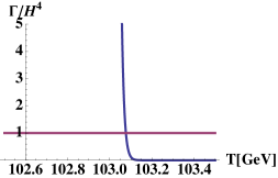
First, we investigate how the percolation is influenced by the vacuum energy. Here we consider typical cases in the Minimal Supersymmetric Standard Model (MSSM) as a specific example (see Appendix A for the details). If we ignore the vacuum energy, we have obtained in order to complete the percolation as is shown in Fig. 1.
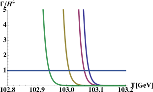
Next we incorporate the effect of the vacuum energy in this setup. For a concrete calculation, we calculate by parameterizing the vacuum energy . As seen in the previous section, the bubble nucleation is determined by the value of the euclidean action. However, there is no effect from the vacuum energy on the nucleation because the constant term is renormalized in the definition of the nucleation rate. Only the Hubble parameter, with Planck mass, should be changed by adding the vacuum energy to the total energy density . The result is plotted in Fig. 2. As seen in this figure, the effect is only a mild change on with a small difference by the order of . That is because the bubble nucleation has the exponential dependence on , which is the dominant contribution to possibly change .
4 Detectability of relic gravitational wave
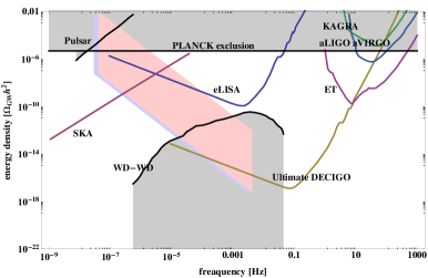
In this section, we discuss detectabilities of the relic gravitational wave background produced at the electroweak phase transition by using two fundamental parameters and . In case of the phase transition at the electroweak scale, the useful experiments should be eLISA [27], Ultimate DECIGO [28, 29, 30] and SKA [31]. The sensitivities of the experiments are summarized in Refs. [30, 44]
There is also a limit from non-detections of extra radiation through the CMB observation such as the Planck satellite experiments as an additional constraint. The extra radiation like the stochastic gravitational background can be measured as a deviation of the effective number of the neutrino species from three to be . Then the energy fraction of the extra radiation at present can be expressed by . So far the Planck collaborations have reported that observationally they had an upper bound on to be . [45]. Then we obtain an upper bound on the energy fraction of the relic gravitational wave background,
| (4.1) |
This is effective over a broad range of frequencies for , 888Or the range is represented in terms of the comoving wave number to be Mpc through . which is wider than the one obtained by big-bang nucleosynthesis (BBN).
We calculate the spectra by changing the parameters to be , and with the transition temperature 70 GeV and 100 GeV with .
In case of the bubble collision, we plot the obtained signals in Fig. 4. The peak frequency is controlled only by . On the other hand, the peak signal is determined by both and . There exist regions which have been already excluded by the Planck constraint [Eq. (4.1)]. It is remarkable that there are parameter regions, which only SKA can observe at a small .
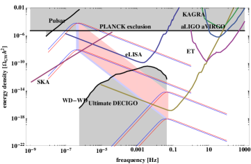
In Fig. 5, we plot the signals of the relic gravitational wave background sourced by the turbulence. Contrary to the case of the bubble collision, it is notable that the peak frequency depends on both and . Of course, the peak signal is also determined by both and . The turbulence makes an important contribution to the signal and has larger detectable parameter regions999By recent hydrodynamic simulations, e.g., [37, 47, 48], it was pointed out that its contribution might be smaller..
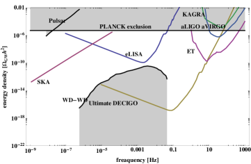
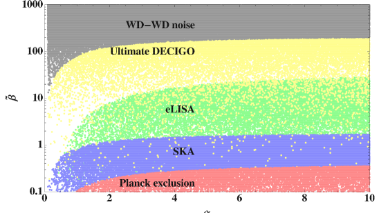
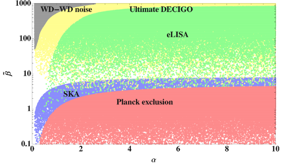
We scanned parameter regions in terms of detectabilities in the () plane. In Fig. 6 the case of the bubble collision is plotted. Here, we consider only the case of . It displays the three regions that can be detected in three experiments (Ultimate DECIGO, eLISA and SKA). The excluded regions by the Plank [Eq. (4.1)] is also plotted at the bottom. Top regions are covered by the WD-WD noise. We have checked that the allowed region does not change much even if we consider the corresponding tail of the full spectrum shown in Eq. (2.24). In Fig. 7, we also plot the case of the turbulence.
5 Conclusions
After the discovery of the Higgs boson, particle physicists in the world tend to get momentum to tackle the physics at the electroweak phase transition head-on and approach a various serious problems related the Higgs sector in detail. Therefore, it is attractive to revisit a variety of possible scenarios for the electroweak phase transition. We have examined detectabilities of the stochastic gravitational wave background produced by the first-order electroweak phase transition in a general setup with carefully considering effects of the vacuum energy on the expansion of the universe.
We have shown that the relic gravitational wave background produced at the electroweak epoch will be observed by the future experiments, such as SKA, eLISA and DECIGO. In particular, the small regions, which is naturally predicted in some particle physics models such as MSSM, will be able to be searched by SKA very near future.
Acknowledgments
We would like to thank Kenta Hotokezaka, Kunihito Ioka, and Eibun Senaha for useful discussions. This work is partially supported by the Grant-in-Aid for Scientific research from the Ministry of Education, Science, Sports, and Culture, Japan, Nos. 25.2309 (Y.K), and 21111006, 22244030, 23540327, 26105520 (K.K.). The work of K.K. is also supported by the Center for the Promotion of Integrated Science (CPIS) of Sokendai (1HB5804100).
Appendix A Scalar sector in MSSM
In this section we show details of the adopted models which are motivated by MSSM [3]. Those models are used to calculate specific physical variables in Sec 3. We refer only a scalar potential required here to be with a constant vacuum energy . The effective potential is then represented by [3]
| (A.1) |
The tree level potential depends only on the scalar field.
| (A.2) |
with being the Higgs mass and being the vev of the Higgs field.
is calculated at the thermal one-loop level. The following is a result of the high temperature expansion,
| (A.3) | |||||
where the number of colors , with , , and being masses of the top quark, the scalar top quark, the boson and the boson, respectively. Here we introduced
| (A.4) | ||||
| (A.5) | ||||
| (A.6) |
where and are the gauge coupling constants, is the strong gauge coupling constant, is the top Yukawa coupling, is the model parameter of the soft-mass squared, and is an angle defined by to be the ratio of two Higgs’ vevs. Finally, is calculated by the two loop effect by incorporating the effect of weak boson and scalar top quark (stop),
| (A.7) |
References
- [1] P. A. R. Ade et al. [BICEP2 Collaboration], arXiv:1403.3985 [astro-ph.CO].
- [2] K. Kajantie, K. Rummukainen and M. E. Shaposhnikov, Nucl. Phys. B 407, 356 (1993), Z. Fodor, J. Hein, K. Jansen, A. Jaster and I. Montvay, Nucl. Phys. B 439, 147 (1995), K. Kajantie, M. Laine, K. Rummukainen and M. E. Shaposhnikov, Nucl. Phys. B 466, 189 (1996), K. Jansen, Nucl. Phys. Proc. Suppl. 47, 196 (1996), B. Bergerhoff and C. Wetterich, Nucl. Phys. B 440, 171 (1995).
- [3] R. Apreda, M. Maggiore, A. Nicolis and A. Riotto, Nucl. Phys. B 631, 342 (2002).
- [4] W. Huang, Z. Kang, J. Shu, P. Wu and J. M. Yang, arXiv:1405.1152 [hep-ph]
- [5] T. Hambye and A. Strumia, Phys. Rev. D 88, 055022 (2013).
- [6] T. Cohen, D. E. Morrissey and A. Pierce, Phys. Rev. D 86, 013009 (2012).
- [7] D. Curtin, P. Jaiswal and P. Meade, JHEP 1208, 005 (2012).
- [8] M. Carena, G. Nardini, M. Quiros and C. E. M. Wagner, JHEP 1302, 001 (2013).
- [9] K. Krizka, A. Kumar and D. E. Morrissey, Phys. Rev. D 87, no. 9, 095016 (2013).
- [10] M. Pietroni, Nucl. Phys. B 402, 27 (1993).
- [11] S. J. Huber and M. G. Schmidt, Nucl. Phys. B 606, 183 (2001).
- [12] J. Kang, P. Langacker, T. -j. Li and T. Liu, Phys. Rev. Lett. 94, 061801 (2005).
- [13] A. Menon, D. E. Morrissey and C. E. M. Wagner, Phys. Rev. D 70, 035005 (2004).
- [14] K. Funakubo, S. Tao and F. Toyoda, Prog. Theor. Phys. 114, 369 (2005).
- [15] S. J. Huber, T. Konstandin, T. Prokopec and M. G. Schmidt, Nucl. Phys. B 757, 172 (2006).
- [16] S. W. Ham, E. J. Yoo and S. K. OH, Phys. Rev. D 76, 075011 (2007).
- [17] S. W. Ham and S. K. OH, Phys. Rev. D 76, 095018 (2007).
- [18] A. Ashoorioon and T. Konstandin, JHEP 0907, 086 (2009).
- [19] C. -W. Chiang and E. Senaha, JHEP 1006, 030 (2010).
- [20] J. Kang, P. Langacker, T. Li and T. Liu, JHEP 1104, 097 (2011).
- [21] A. Ahriche and S. Nasri, Phys. Rev. D 83, 045032 (2011).
- [22] M. Carena, N. R. Shah and C. E. M. Wagner, Phys. Rev. D 85, 036003 (2012).
- [23] K. Cheung, T. -J. Hou, J. S. Lee and E. Senaha, Phys. Lett. B 710, 188 (2012).
- [24] J. Kozaczuk, S. Profumo and C. L. Wainwright, Phys. Rev. D 87, no. 7, 075011 (2013).
- [25] E. Senaha, Phys. Rev. D 88, no. 5, 055014 (2013).
- [26] G. Aad et al. [ATLAS Collaboration], Phys. Lett. B 716, 1 (2012). S. Chatrchyan et al. [CMS Collaboration], Phys. Lett. B 716, 30 (2012).
- [27] https://www.elisascience.org
- [28] N. Seto, S. Kawamura and T. Nakamura, Phys. Rev. Lett. 87, 221103 (2001).
- [29] H. Kudoh, A. Taruya, T. Hiramatsu and Y. Himemoto, Phys. Rev. D 73, 064006 (2006).
- [30] L. Alabidi, K. Kohri, M. Sasaki and Y. Sendouda, JCAP 1305, 033 (2013).
- [31] M. Kramer and B. Stappers, arXiv:1009.1938 [astro-ph.IM], Proceedings of the ISKAF2010 Science Meeting (2010) Assen, Netherlands
- [32] https://www.skatelescope.org/project/projecttimeline/
- [33] J. Kehayias and S. Profumo, JCAP 1003, 003 (2010).
- [34] A. Kosowsky, M. S. Turner and R. Watkins, Phys. Rev. D 45, 4514 (1992).
- [35] C. Caprini, R. Durrer and G. Servant, Phys. Rev. D 77, 124015 (2008) [arXiv:0711.2593 [astro-ph]].
- [36] A. Kosowsky and M. S. Turner, Phys. Rev. D 47, 4372 (1993).
- [37] M. Hindmarsh, S. J. Huber, K. Rummukainen and D. J. Weir, Phys. Rev. Lett. 112, 041301 (2014).
- [38] C. Grojean and G. Servant, Phys. Rev. D 75, 043507 (2007).
- [39] C. Caprini, R. Durrer and G. Servant, JCAP 0912, 024 (2009) [arXiv:0909.0622 [astro-ph.CO]].
- [40] A. D. Linde, Nucl. Phys. B 216, 421 (1983) [Erratum-ibid. B 223, 544 (1983)].
- [41] L. Sagunski, DESY-THESIS-2013-011.
- [42] M. Kamionkowski, A. Kosowsky and M. S. Turner, Phys. Rev. D 49, 2837 (1994).
- [43] S. J. Huber and T. Konstandin, JCAP 0809, 022 (2008).
- [44] T. Regimbau, T. Dent, W. Del Pozzo, S. Giampanis, T. G. F. Li, C. Robinson, C. Van Den Broeck and D. Meacher et al., Phys. Rev. D 86, 122001 (2012).
- [45] P. A. R. Ade et al. [Planck Collaboration], arXiv:1303.5076 [astro-ph.CO].
- [46] R. Schneider, S. Marassi and V. Ferrari, Class. Quant. Grav. 27, 194007 (2010) [arXiv:1005.0977 [astro-ph.CO]].
- [47] J. T. Giblin and J. B. Mertens, arXiv:1405.4005 [astro-ph.CO].
- [48] J. R. Espinosa, T. Konstandin, J. M. No and G. Servant, JCAP 1006, 028 (2010) [arXiv:1004.4187 [hep-ph]].