Sequential Monte Carlo with Highly Informative Observations

Abstract

We propose sequential Monte Carlo (SMC) methods for sampling the posterior distribution of state-space models under highly informative observation regimes, a situation in which standard SMC methods can perform poorly. A special case is simulating bridges between given initial and final values. The basic idea is to introduce a schedule of intermediate weighting and resampling times between observation times, which guide particles towards the final state. This can always be done for continuous-time models, and may be done for discrete-time models under sparse observation regimes; our main focus is on continuous-time diffusion processes. The methods are broadly applicable in that they support multivariate models with partial observation, do not require simulation of the backward transition (which is often unavailable), and, where possible, avoid pointwise evaluation of the forward transition. When simulating bridges, the last cannot be avoided entirely without concessions, and we suggest an $\epsilon$-ball approach (reminiscent of Approximate Bayesian Computation) as a workaround. Compared to the bootstrap particle filter, the new methods deliver substantially reduced mean squared error in normalising constant estimates, even after accounting for execution time. The methods are demonstrated for state estimation with two toy examples, and for parameter estimation (within a particle marginal Metropolis–Hastings sampler) with three applied examples in econometrics, epidemiology and marine biogeochemistry.

1 Introduction

Consider the multivariate and continuous-time Markov process $X(t)\in\mathbb{R}^{d}$ and parameters $\Theta$. For a sequence of times $t_{0},\ldots,t_{n}$ we write $X_{0:n}\equiv\{X_{0},\ldots,X_{n}\}\equiv\{X(t_{0}),\ldots,X(t_{n})\}$, and adopt the convention that uppercase symbols denote random variables, with matching lowercase symbols realisations of them. We have $X_{k}\sim p(dx_{k}\,|\,x_{k-1},\theta)$. The process may be observed indirectly via some $Y_{n}\sim p(dy_{n}\,|\,x_{n},\theta)$, or directly as some given initial value $x_{0}$ and final value $x_{n}$. This setup admits continuous-time models, where $n$ can be made arbitrarily large and so $t_{1},\ldots,t_{n-1}$ arbitrarily dense, and discrete-time models with sparse observation, where $n$ cannot be made arbitrarily large, but where times $t_{1},\ldots,t_{n-1}$ are unobserved.

In the case of indirect observation, the problem of interest is to simulate $X_{0:n}\sim p(dx_{0:n}\,|\,y_{n},\theta)$ and perhaps estimate the normalising constant (marginal likelihood) $p(y_{n}\,|\,\theta)$. We are particularly interested in the case that the observation is in some sense highly informative on $X_{0:n}$. This might arise when highly accurate measurements are taken in controlled settings, or where observations are relatively sparse in time. It will be adequate in this work for the meaning of “highly informative” to remain qualitative—vague even—but if it were to be quantified it might be defined as some large divergence (e.g. Kullback–Leibler) of $p(dx_{n}\,|\,\theta)$ from $p(dx_{n}\,|\,y_{n},\theta)$.

In the case of direct observation, the problem of interest is to simulate bridges $X_{1:n-1}\sim p(dx_{1:n-1}\,|\,x_{0},x_{n},\theta)$ and perhaps estimate the normalising constant (transition density) $p(x_{n}\,|\,x_{0},\theta)$. This might be seen as the special case of indirect observation with $p(y_{n}\,|\,x_{n})=\delta(y_{n}-x_{n})$, where $\delta$ is the Dirac $\delta$ function. We motivate the approach with this special case, and return to the more general case later.

The simulation of bridges is generally regarded as a difficult problem, and there is a wealth of literature in the area. Most approaches, while not necessarily limited to such, begin with a diffusion process satisfying the Itô stochastic differential equation (SDE)

$$dX(t)=a(X(t),t,\theta)\,dt+B(X(t),t,\theta)\,dW(t),$$

where $a(X(t),t,\theta)$ is the drift vector, $B(X(t),t,\theta)$ the diffusion matrix and $W(t)$ a vector of standard Wiener processes. One group of methods proceeds with a schedule of times $t_{0},\ldots,t_{n}$, equispaced at a sufficiently small step size that a locally linear–Gaussian Euler–Maruyama (Kloeden and Platen, 1992, §9.1) discretisation of the original dynamics makes a credible approximation:

$$p(x_{k}\,|\,x_{k-1},\theta):=\mathcal{\phi}\left(x_{k-1}+a(x_{k-1},t_{k-1},\theta)\Delta t_{k},\,B(x_{k-1},t_{k-1},\theta)B(x_{k-1},t_{k-1},\theta)^{\top}\Delta t_{k}\right).$$

Here, $k=1,\ldots,n$, $\Delta t_{k}=t_{k}-t_{k-1}$ and $\phi(\mu,\Sigma)$ is the probability density function of the normal distribution with mean vector $\mu$ and covariance matrix $\Sigma$. Because of the convenience of this closed form for $p(x_{k}\,|\,x_{k-1},\theta)$, the discretised version may be adopted in place of the continuous version (as an a priori approximation) before proceeding with inference. This facilitates various importance sampling (e.g. Pedersen, 1995; Durham and Gallant, 2002), sequential Monte Carlo (SMC, e.g. Lin et al., 2010) and Markov chain Monte Carlo (MCMC, e.g. Roberts and Stramer, 2001; Elerian et al., 2001; Eraker, 2001; Golightly and Wilkinson, 2006) methods for simulating bridges.

A caution is warranted around the use of Euler–Maruyama, however. While the discretisation provides a convenient approximation for pointwise evaluation of $p(x_{k}\,|\,x_{k-1},\theta)$, it can be unstable for simulation unless the step size is very small—too small for efficient computation. In such cases higher-order schemes, such as the Milstein and semi-implicit schemes (Kloeden and Platen, 1992), or those of the Runge–Kutta family, are to be preferred, and indeed may be essential. For any given step size $\Delta t$, these higher-order schemes have stability regions at least as large as that of Euler–Maruyama. For particularly stiff problems, implicit schemes may also need to be considered.

Rather than discretising to yield a closed-form transition density, a closed-form Radon–Nikodym derivative can be derived in certain conditions. This leads to another family of methods for simulating bridges (e.g. Clark, 1990; Delyon and Hu, 2006; Bayer and Schoenmakers, 2013; Schauer et al., 2013). The exact algorithm (Beskos et al., 2006) is yet another alternative, and has the advantage of not introducing discretisation error, but its requirements restrict the set of models to which it can be applied, especially the set of multivariate models.

The estimation of the normalising constant $p(x_{n}\,|\,x_{0},\theta)$ usually falls out as a straightforward expectation in importance sampling methods, including SMC. It is more difficult with MCMC. A number of works have focused more closely on this, usually in the context of obtaining normalising constant estimates for parameter estimation (e.g. Fearnhead et al., 2008, 2010; Sun et al., 2013).

The methods proposed in this work are most similar to the SMC methods of Del Moral and Garnier (2005), and Lin et al. (2010). The former considers the simulation of rare events, not bridges, albeit with similar mechanisms. The latter does consider the simulation of bridges, but the implementation has some limitations, which this work seeks to ameliorate. In particular, Lin et al. (2010) requires that pilot samples can be initialised at time $t_{n}$ and simulated backwards in time to guide those samples being simulated forwards in time. This is problematic in cases where the backwards transition cannot be discretised in a numerically stable way. In contrast, the proposed methods do not require simulation of the backwards transition. In addition, Lin et al. (2010) does not support indirect observation, and in the case of multivariate models and direct observation, does not support partial observation of the state vector $x_{n}$. The proposed methods accommodate both of these cases. In the context of indirect observation, the methods are similar to the auxiliary particle filter (Pitt and Shephard, 1999), but perform lookahead steps at multiple intermediate times between observations, rather than at observation times only.

The remainder of this work describes the proposed methods for sampling from state-space models with highly informative observations, including the special case of simulating bridges. The methods also permit estimation of normalising constants. The basic idea is to simulate particles forward in time using only the prior $p(dx_{k}\,|\,x_{k-1},\theta)$, discretised with a higher-order scheme, but to introduce additional weighting and resampling steps at intermediate times to guide particles towards the final state. The methods are simple to apply, with the following properties that make them useful for a broad range of problems:

1. They work in a multivariate setting.

2. They support partial observation of the state vector $x_{n}$.

3. They do not require that the backward transition can be simulated.

4. They support higher-order discretisations of the forward state process than that of Euler–Maruyama.

5. They require only that the forward transition can be simulated and not that its probability density function $p(x_{k}\,|\,x_{k-1},\theta)$ can be evaluated pointwise. This comes with the caveat that in the special case of simulating bridges, a workaround is needed to approximately evaluate, or avoid the evaluation of, $p(x_{n}\,|\,x_{n-1},\theta)$. In one example we use an Euler–Maruyama discretisation to approximately evaluate, but not simulate, $p(x_{n}\,|\,x_{n-1},\theta)$. In another we concede an $\epsilon$-ball around $x_{n}$, where $\epsilon$ is commensurate with the discretisation error already surrendered by the numerical integrator. The latter strategy resembles a simple Approximate Bayesian Computation (ABC) algorithm (Beaumont et al., 2002).

Three methods are introduced in this work, all similar but tailored for slightly different circumstances. §2 provides the formal background to establish the methods. §3 provides pseudocode for their implementation and discusses design of the required weight functions. §4 provides empirical results for the methods on two toy examples and three applications in econometrics, epidemiology and marine biogeochemistry. §5 draws these results together and reports on experiences in tuning the methods. §6 concludes.

2 Methods

We derive three methods in this section, all quite related, but for different circumstances of the model and data. References to the parameters, $\Theta$, are omitted throughout for brevity. Likewise, observation of the final value $x_{n}$ may be full or partial; the methods support both cases, but for simplicity no notational distinction is made.

Firstly note:

$$p(x_{1:n-1}\,|\,x_{0},x_{n}) = \frac{p(x_{n}\,|\,x_{n-1})p(x_{1:n-1}\,|\,x_{0})}{p(x_{n}\,|\,x_{0})}$$

$$\propto p(x_{n}\,|\,x_{n-1})p(x_{1:n-1}\,|\,x_{0}).$$

This forms the basis of the importance sampling method of Pedersen (1995), proposing from $p(dx_{1:n-1}\,|\,x_{0})$ and weighting with $p(x_{n}\,|\,x_{n-1})$. The use of the prior as the proposal in this way is myopic of $x_{n}$, and while often workable, the approach can lead to excessive variance in importance weights and subsequent computational expense. In Durham and Gallant (2002), an alternative proposal is suggested, adjusting the drift term of the SDE with a linear component to draw the process towards $x_{n}$. The transition densities $p(x_{k}\,|\,x_{k-1})$ must then be estimated in order to compute weights, and the low-order Euler–Maruyama discretisation is employed to achieve this. One, perhaps overlooked, advantage of Pedersen (1995) is that $p(x_{k}\,|\,x_{k-1})$ does not need to be evaluated pointwise except for the weight at $k=n$. This means that, for the purposes of simulation, higher-order discretisation schemes can be admitted. The methods of this work enjoy the same property.

Further observe:

$$p(x_{1:n-1}\,|\,x_{0})=\prod_{k=1}^{n-1}p(x_{k}\,|\,x_{k-1})$$ (1)

and

$$\frac{p(x_{n}\,|\,x_{n-1})}{p(x_{n}\,|\,x_{0})}=\prod_{k=1}^{n-1}\frac{p(x_{n}\,|\,x_{k})}{p(x_{n}\,|\,x_{k-1})},$$ (2)

and define

$$G_{k}(x_{k-1:k}):=\frac{p(x_{n}\,|\,x_{k})}{p(x_{n}\,|\,x_{k-1})}.$$

One can then incrementally simulate $p(dx_{k}\,|\,x_{k-1})$ and weight with $G_{k}(x_{k-1:k})$, for $k=1,\ldots,n-1$. The basis of an SMC method is to do precisely this, maintaining a population of samples (particles) and introducing a selection mechanism to resample from amongst them, according their weights, at each increment. Lin et al. (2010) does this; the development below follows a similar path, but we will ultimately suggest a different implementation, and extend the idea from the special case of sampling bridges to the more general case of sampling under highly informative observations.

Proposition 1.

For any bounded function $f$ on $(\mathbb{R}^{d})^{n-1}$, we have

$$\mathbb{E}\left[f(X_{1:n-1})\,|\,x_{0},x_{n}\right] = \mathbb{E}\left[f(X_{1:n-1})\prod_{k=1}^{n-1}G_{k}(X_{k-1:k})\,\middle|\,x_{0}\right]$$

with the weight functions

$$G_{k}(x_{k-1:k}):=\frac{p(x_{n}\,|\,x_{k})}{p(x_{n}\,|\,x_{k-1})}.$$

Proof.

The conditional density of the random path $X_{1:n-1}$ given initial state $X_{0}=x_{0}$ and final value $X_{n}=x_{n}$ is

$$p(x_{1:n-1}\,|\,x_{0},x_{n}) = \frac{{\displaystyle p(x_{n}\,|\,x_{n-1})p(x_{1:n-1}\,|\,x_{0})}}{p(x_{n}\,|\,x_{0})}$$

$$= {\displaystyle\left\{\prod_{k=1}^{n-1}\frac{p(x_{n}\,|\,x_{k})}{p(x_{n}\,|\,x_{k-1})}\right\}p(x_{1:n-1}\,|\,x_{0})}$$

$$= \left\{\prod_{k=1}^{n-1}G_{k}(x_{k-1:k})\right\}p(x_{1:n-1}\,|\,x_{0}).$$

Thus for any bounded function $f$ on $(\mathbb{R}^{d})^{n-1}$ we have

$$\mathbb{E}\left[f(X_{1:n-1})\,|\,x_{0},x_{n}\right] = \int_{\mathbb{R}^{d(n-1)}}f(x_{1:n-1})p(x_{1:n-1}\,|\,x_{0},x_{n})\,dx_{1:n-1}$$

$$= \int_{\mathbb{R}^{d(n-1)}}f(x_{1:n-1})\left\{\prod_{k=1}^{n-1}G_{k}(x_{k-1:k})\right\}p(x_{1:n-1}\,|\,x_{0})\,dx_{1:n-1}$$

$$= \mathbb{E}\left[f(X_{1:n-1})\prod_{k=1}^{n-1}G_{k}(X_{k-1:k})\,\middle|\,x_{0}\right].$$

∎

Of course, rarely will the weights $G_{k}(x_{k-1:k})$ be computable in practice; Proposition 1 is conceptually appealing, however, and we can try to imitate it in other circumstances. To do this, we introduce arbitrary weighting functions that facilitate an SMC algorithm.

Proposition 2.

For any bounded function $f$ on $(\mathbb{R}^{d})^{n-1}$, we have

$$\begin{array}[]{l}\mathbb{E}\left[f(X_{1:n-1})\,|\,x_{0},x_{n}\right]={\displaystyle\frac{\mathbb{E}\left[f(X_{1:n-1})p(x_{n}\,|\,X_{n-1})\frac{q(x_{n}\,|\,x_{0})}{q(x_{n}\,|\,X_{n-1})}\prod_{k=1}^{n-1}H_{k}(X_{k-1:k})\,\middle|\,x_{0}\right]}{\mathbb{E}\left[p(x_{n}\,|\,X_{n-1})\frac{q(x_{n}\,|\,x_{0})}{q(x_{n}\,|\,X_{n-1})}\prod_{k=1}^{n-1}H_{k}(X_{k-1:k})\,\middle|\,x_{0}\right]}}\end{array}.$$

with the weight functions

$$H_{k}(x_{k-1:k}):=\frac{q(x_{n}\,|\,x_{k})}{q(x_{n}\,|\,x_{k-1})}$$

and chosen positive functions $q(x_{n}\,|\,x_{k})$ for $k=0,\ldots,N-1$.

Proof.

Observe that

$$p(x_{n}\,|\,x_{0})=\mathbb{E}\left[p(x_{n}\,|\,X_{n-1})\,\middle|\,x_{0}\right]$$

so that

$$\mathbb{E}\left[f(X_{1:n-1})\,|\,x_{0},x_{n}\right] = \mathbb{E}\left[f(X_{1:n-1})\frac{p(x_{n}\,|\,X_{n-1})}{p(x_{n}\,|\,x_{0})}\,\middle|\,x_{0}\right]$$

$$= \frac{\mathbb{E}\left[f(X_{1:n-1})p(x_{n}\,\middle|\,X_{n-1})\,|\,x_{0}\right]}{p(x_{n}\,|\,x_{0})}$$

$$= \frac{\mathbb{E}\left[f(X_{1:n-1})p(x_{n}\,\middle|\,X_{n-1})\,|\,x_{0}\right]}{\mathbb{E}\left[p(x_{n}\,|\,X_{n-1})\,\middle|\,x_{0}\right]}.$$

Introduce

$$\frac{q(x_{n}\,|\,x_{0})}{q(x_{n}\,|\,x_{n-1})}\prod_{k=1}^{n-1}H_{k}(x_{k-1:k})=1.$$

We then have

$$\mathbb{E}\left[f(X_{1:n-1})\,|\,x_{0},x_{n}\right] = \frac{\mathbb{E}\left[f(X_{1:n-1})p(x_{n}\,|\,X_{n-1})\frac{q(x_{n}\,|\,x_{0})}{q(x_{n}\,|\,X_{n-1})}\prod_{k=1}^{n-1}H_{k}(X_{k-1:k})\,\middle|\,x_{0}\right]}{\mathbb{E}\left[p(x_{n}\,|\,X_{n-1})\frac{q(x_{n}\,|\,x_{0})}{q(x_{n}\,|\,X_{n-1})}\prod_{k=1}^{n-1}H_{k}(X_{k-1:k})\,\middle|\,x_{0}\right]}.$$

∎

The results are easily adapted to the case where the state is not observed exactly, but rather with some noise. We introduce the random variable $Y_{n}\sim p(dy_{n}\,|\,x_{n})$, which will be observed in place of $X_{n}$, and a prior distribution over the starting state, $X_{0}\sim p(dx_{0})$.

Proposition 3.

For any bounded function $f$ on $\mathbb{R}^{d(n+1)}$, we have

$$\begin{array}[]{l}\mathbb{E}\left[f(X_{0:n})\,|\,y_{n}\right]={\displaystyle\frac{\mathbb{E}\left[f(X_{0:n})p(X_{0})p(y_{n}\,|\,X_{n})\frac{r(y_{n}\,|\,X_{0})}{r(y_{n}\,|\,X_{n})}\prod_{k=1}^{n}J_{k}(X_{k-1:k})\right]}{\mathbb{E}\left[p(X_{0})p(y_{n}\,|\,X_{n})\frac{r(y_{n}\,|\,X_{0})}{r(y_{n}\,|\,X_{n})}\prod_{k=1}^{n}J_{k}(X_{k-1:k})\right]}}\end{array}.$$

with the weight functions

$$J_{k}(x_{k-1:k}):=\frac{r(y_{n}\,|\,x_{k})}{r(y_{n}\,|\,x_{k-1})}$$

and chosen positive functions $r(y_{n}\,|\,x_{k})$ for $k=0,\ldots,N$.

Proof.

Observe that

$$p(y_{n})=\mathbb{E}\left[p(y_{n}\,|\,X_{n})\right]$$

so that

$$\mathbb{E}\left[f(X_{0:n})\,|\,y_{n}\right] = \mathbb{E}\left[f(X_{0:n})\frac{p(y_{n}\,|\,X_{n})}{p(y_{n})}\right]$$

$$= \frac{\mathbb{E}\left[f(X_{0:n})p(y_{n}\,|\,X_{n})\right]}{p(y_{n})}$$

$$= \frac{\mathbb{E}\left[f(X_{0:n})p(y_{n}\,|\,X_{n})\right]}{\mathbb{E}\left[p(y_{n}\,|\,X_{n})\right]}.$$

Introduce

$$\frac{r(y_{n}\,|\,x_{0})}{r(y_{n}\,|\,x_{n})}\prod_{k=1}^{n}J_{k}(x_{k-1:k})=1,$$

We then have

$$\mathbb{E}\left[f(X_{0:n})\,|\,y_{n}\right] = {\displaystyle\frac{\mathbb{E}\left[f(X_{0:n})p(X_{0})p(y_{n}\,|\,X_{n})\frac{r(y_{n}\,|\,X_{0})}{r(y_{n}\,|\,X_{n})}\prod_{k=1}^{n}J_{k}(X_{k-1:k})\right]}{\mathbb{E}\left[p(X_{0})p(y_{n}\,|\,X_{n})\frac{r(y_{n}\,|\,X_{0})}{r(y_{n}\,|\,X_{n})}\prod_{k=1}^{n}J_{k}(X_{k-1:k})\right]}}$$

∎

We expect this modification to lead to an SMC algorithm that is particularly useful when observations are highly informative.

3 Implementation

The recursive structure of the weight functions in Propositions 1–3 and Markov property of the process $X(t)$ facilitate SMC algorithms to compute the expectations of interest. Such algorithms propagate, weight and resample a population of $N$ particles. We present Algorithms 1–3 as pseudocode, corresponding to Propositions 1–3, respectively. Where a superscript $i$ appears on the left-hand side of an assignment in these algorithms, the intended interpretation is “for all $i\in\left\{1,\ldots,N\right\}$”. The left arrow notation ($\leftarrow$) denotes assignment of the value on the right to the variable on the left, while the tilde notation ($\sim$) denotes assignment of a draw from the distribution on the right to the variable on the left. We start with Algorithm 1, corresponding to Proposition 1:

Algorithm 1.

• $x^{i}_{0}\leftarrow x_{0}$ // initialise $w^{i}_{0}\leftarrow 1/N$ for $k=1,\ldots,n-1$ if resampling is triggered $a^{i}_{k}\sim R(da_{k}\,|\,w^{1:N}_{k-1})$ // select $w^{i}_{k}\leftarrow 1/N$ else $a^{i}_{k}\leftarrow i$ $w^{i}_{k}\leftarrow w^{i}_{k-1}/\sum_{j}^{N}w^{j}_{k-1}$ $x^{i}_{k}\sim p(dx_{k}\,|\,x^{a^{i}_{k}}_{k-1})$ // propagate $w^{i}_{k}\leftarrow p(x_{n}\,|\,x^{i}_{k})\cdot w^{i}_{k}/w^{a^{i}_{k}}_{k-1}$ // weight

Algorithm 2, corresponding to Proposition 2, is given below. It assumes that $q(x_{n}\,|\,x_{n-1}):=p(x_{n}\,|\,x_{n-1})$. Note that Algorithm 1 is just the special case of Algorithm 2 where $q(x_{n}\,|\,x_{k}):=p(x_{n}\,|\,x_{k})$.

Algorithm 2.

• $x^{i}_{0}\leftarrow x_{0}$ // initialise $w^{i}_{0}\leftarrow 1/N$ for $k=1,\ldots,n-1$ if resampling is triggered $a^{i}_{k}\sim R(da_{k}\,|\,w^{1:N}_{k-1})$ // select $w^{i}_{k}\leftarrow 1/N$ else $a^{i}_{k}\leftarrow i$ $w^{i}_{k}\leftarrow w^{i}_{k-1}/\sum_{j}^{N}w^{j}_{k-1}$ $x^{i}_{k}\sim p(dx_{k}\,|\,x^{a^{i}_{k}}_{k-1})$ // propagate $w^{i}_{k}\leftarrow q(x_{n}\,|\,x^{i}_{k})\cdot w^{i}_{k}/w^{a^{i}_{k}}_{k-1}$ // weight

At the conclusion of Algorithm 1 or 2, let $b_{n-1}^{i}=i$ and, recursively, $b_{k}^{i}=a_{k+1}^{b_{k+1}^{i}}$. The indices $b_{k}^{i}$ then establish ancestral lines

$$x_{0}\rightarrow x_{1}^{b_{1}^{i}}\rightarrow x_{2}^{b_{2}^{i}}\rightarrow\cdots\rightarrow x_{n-2}^{b_{n-2}^{i}}\rightarrow x_{n-1}^{b_{n-1}^{i}}\rightarrow x_{n}.$$

Because SMC methods are a particular case of mean field particle methods (Del Moral, 2004), these may be used to compute expectations of the forms that appear in Propositions 1 and 2:

$$\frac{\sum_{i=1}^{N}w_{n-1}^{i}f\left(x_{1}^{b_{1}^{i}},\ldots,x_{n-1}^{b_{n-1}^{i}}\right)}{\sum_{i=1}^{N}w_{n-1}^{i}} \underset{N\uparrow\infty}{\longrightarrow} \mathbb{E}\left[f(X_{1:n-1})\,|\,x_{0},x_{n}\right].$$

The denominator on the left is also an estimate of the normalising constant:

$$\sum_{i=1}^{N}w_{n-1}^{i} \underset{N\uparrow\infty}{\longrightarrow} \mathbb{E}\left[p(x_{n}\,|\,X_{n-1})\,\middle|\,x_{0}\right]$$

$$= p(x_{n}\,|\,x_{0}).$$

Note that as Algorithms 1 and 2 normalise the weights $w_{n-1}^{1:N}$ after the selection step but before the weighting step, no factor of $1/N$ appears outside the summation in (3).

It is often the case that the transition density $p(x_{n}\,|\,x_{n-1})$ does not have a convenient closed form for pointwise evaluation, so that the last line of Algorithm 2 cannot be evaluated. In such cases one of two approaches might be considered. In the first approach, the sequence of times $t_{1},\ldots,t_{n-1}$ might be set so that the last interval, $\Delta t_{n}=t_{n}-t_{n-1}$, is sufficiently small for the Euler–Maruyama approximation of $p(x_{n}\,|\,x_{n-1})$ to be credible. Because this last transition is evaluated but not simulated (much less simulated repeatedly with accumulating error), the stability issues of the Euler–Maruyama discretisation will not manifest. In the second approach, an observation model might be constructed with an $\epsilon$-ball around $x_{n}$, where $\epsilon$ is commensurate with the discretisation error already inherent in the numerical integrator. We do this in the SIR example of §4.

This second approach yields an algorithm resembling ABC (Beaumont et al., 2002). In a simple ABC algorithm, one would simulate a path $x^{\prime}_{1:n}\sim p(dx_{1:n}\,|\,x_{0})$ and accept it if $\rho(x^{\prime}_{n},x_{n})\leq\epsilon$ for some distance function $\rho$ and error threshold $\epsilon$. The SMC component of the proposed method marginalises over multiple such paths. If we define the unnormalised density

$$p(x_{n}\,|\,x_{n-1}):=\begin{cases}1,&\text{if}\,\rho(x^{\prime}_{n},x_{n})\leq\epsilon\\ 0,&\text{otherwise}\end{cases},$$

then the estimate of the normalising constant (3) is also an estimate of the acceptance probability of $\theta^{\prime}$. It is worth stressing that the SMC component in this case is used in a very different way to ABC SMC methods in the spirit of e.g. Sisson et al. (2007); Beaumont et al. (2009); Del Moral et al. (2012); Peters et al. (2012). In these works, SMC is used over parameters, here it is used over the state. It could be coupled with MCMC (as in particle MCMC, Andrieu et al. 2010) or another level of SMC (as in SMC², Chopin et al. 2013) for parameter estimation, however.

Algorithm 3, corresponding to Proposition 3, is a slight variation on Algorithm 2, as $x_{0}$ and $x_{n}$ are no longer fixed and $y_{n}$ is introduced. It assumes, sensibly, that $r(y_{n}\,|\,x_{n}):=p(y_{n}\,|\,x_{n})$.

Algorithm 3.

• $x^{i}_{0}\sim p(dx_{0})$ // initialise $w^{i}_{0}\leftarrow 1/N$ for $k=1,\ldots,n$ if resampling is triggered $a^{i}_{k}\sim R(da_{k}\,|\,w^{1:N}_{k-1})$ // select $w^{i}_{k}\leftarrow 1/N$ else $a^{i}_{k}\leftarrow i$ $w^{i}_{k}\leftarrow w^{i}_{k-1}/\sum_{j}^{N}w^{j}_{k-1}$ $x^{i}_{k}\sim p(dx_{k}\,|\,x^{a^{i}_{k}}_{k-1})$ // propagate $w^{i}_{k}\leftarrow r(y_{n}\,|\,x^{i}_{k})\cdot w^{i}_{k}/w^{a^{i}_{k}}_{k-1}$ // weight

At the conclusion of Algorithm 3, the indices $b_{k}^{i}$, defined as before, establish ancestral lines

$$x_{0}^{b_{0}^{i}}\rightarrow x_{1}^{b_{1}^{i}}\rightarrow x_{2}^{b_{2}^{i}}\rightarrow\cdots\rightarrow x_{n-2}^{b_{n-2}^{i}}\rightarrow x_{n-1}^{b_{n-1}^{i}}\rightarrow x_{n}^{b_{n}^{i}}.$$

These may be used to compute expectations of the form that appears in Proposition 3:

$$\frac{\sum_{i=1}^{N}w_{n}^{i}f\left(x_{0}^{b_{0}^{i}},\ldots,x_{n}^{b_{n}^{i}}\right)}{\sum_{i=1}^{N}w_{n}^{i}} \underset{N\uparrow\infty}{\longrightarrow} \mathbb{E}\left[f(X_{0:n})\,|\,y_{n}\right].$$

The denominator on the left is also an estimate of the normalising constant:

$$\sum_{i=1}^{N}w_{n}^{i} \underset{N\uparrow\infty}{\longrightarrow} \mathbb{E}\left[p(y_{n}\,|\,X_{n})\right]$$

$$= p(y_{n}).$$

Note that as Algorithm 3 normalises the weights $w_{n}^{1:N}$ after the selection step but before the weighting step, no factor of $1/N$ appears outside the summation in (3).

Algorithm 3 treats the case where there is only a single observation, at time $t_{n}$. This is straightforwardly extended to a time series of observations, where the algorithm is repeated, but removing the first two lines from the second and subsequent iterations; the current particles and their weights are maintained instead. This is then a particle filter, with the addition of intermediate times between observations where additional weighting and resampling is performed to guide particles towards the next state.

3.1 Intermediate weighting

What remains is the selection of appropriate functions $q$ and $r$ in Algorithms 2 and 3. For good performance, we should seek $q(x_{n}\,|\,x_{k})\approx p(x_{n}\,|\,x_{k})$, so that Algorithm 2 approximates Algorithm 1 as closely as possible, and $r(y_{n}\,|\,x_{k})\approx p(y_{n}\,|\,x_{k})$, much like the use of lookahead (Lin et al., 2013) strategies for stage one weights in an auxiliary particle filter (Pitt and Shephard, 1999). As $q(x_{n}\,|\,x_{k})$ and $r(y_{n}\,|\,x_{k})$ play a similar role to the proposal distribution in importance sampling, we should also prefer that their tails are not too tight with respect to $p(x_{n}\,|\,x_{k})$ or $p(y_{n}\,|\,x_{k})$, respectively. For reasons of computational expediency, we suppose that the weight functions are to be selected a priori. Choosing some parametric form, we might choose either to fit the function to simulations of the prior model, or to the data set. We utilise both approaches in the examples of §4.

The implementation in Lin et al. (2010) uses a kernel density estimate of $p(x_{k}\,|\,x_{n})\propto p(x_{n}\,|\,x_{k})p(x_{k})$, obtained by propagating pilot particles backwards from time $t_{n}$ to time $t_{k}$, initialising each at $x_{n}$. This is problematic for the constraints we have given ourselves: it requires that $x_{n}$ is fully observed in order to initialise each particle, it does not support indirect observation, and we do not wish to assume that the backwards transition can be simulated in a numerically stable way.

For diffusion processes, discretisations that provide a closed-form transition density may be useful. As even very approximate weight functions may have some utility, an Euler–Maruyama discretisation might prove useful. More sophisticated Gaussian approximations such as a linear noise approximation (Van Kampen, 2007, p. 258) may also be useful, if more computationally expensive.

We have found that a generally useful approach is to fit a Gaussian process to each observed time series and then construct weight functions based on these;

$$X(t)\sim\mathcal{GP}\left(\mu(t),C(\Delta t)\right),$$

with mean function $\mu(t)$ and covariance function $C(\Delta t)$. This affords a great deal of flexibility in the design of weight functions, accommodating arbitrary mean functions to capture nonlinear drifts, and a variety of covariance functions to capture local behaviour and smoothness. In the examples of §4 it has not been necessary to be too clever to obtain good results: the mean function is always $\mu(t)=0$ and the covariance function of a squared exponential form, parameterised by $\alpha$ and $\beta$;

$$C(\Delta t)=\alpha\exp\left(-\frac{1}{2\beta}(\Delta t)^{2}\right).$$

The parameters $\alpha$ and $\beta$ are set to their maximum likelihood estimates, obtained offline. One can, of course, imagine more sophisticated mean and covariance functions—Gaussian processes being very flexible in this regard—but we have found this simple choice adequate for the examples here. The functions $q(x_{n}\,|\,x_{k})$ are then constructed by conditioning the Gaussian process on the current state, taking

$$q(x_{n}\,|\,x_{k}):=\phi(\mu_{k},\sigma_{k}^{2})$$

with

$$\mu_{k} = \frac{C(t_{n}-t_{k})}{\alpha}x_{k}$$

$$\sigma_{k}^{2} = \alpha-\frac{C(t_{n}-t_{k})^{2}}{\alpha}.$$

Conditioning on the current state only, and not the full state history, is a computational concession, preserving linear complexity in the number of particles $N$. We have found this sufficient for the examples in this work. If necessary, one might consider conditioning on some fixed number of previous states, preserving the same linear complexity. In the case of indirect observation, a (possibly approximate) Gaussian observation model of

$$Y(t)\sim\mathcal{N}(X(t),\varsigma^{2}(t)),$$

for some variance $\varsigma^{2}(t)$, would suggest weight functions of

$$r(y_{n}\,|\,x_{k}):=\phi(\mu_{k},\sigma_{k}^{2}+\varsigma_{n}^{2}).$$

We may be concerned that these tight-tailed Gaussians are too narrow as weight functions, and may be too aggressive in particle selection. A simple precaution is to inflate the variance by some constant factor, and we do this in the examples of §4. One might also consider heavier-tailed functions such as the Student $t$. Another limitation of the Gaussian process formulation is that it may be inadequate for capturing multimodal transition densities. This occurs in the periodic drift example of Section 4, and we propose a bespoke function in that case.

3.2 Intermediate resampling

The intermediate resampling steps require some consideration. In the first instance, they introduce additional computational expense. In the second they may introduce additional variance in normalising constant estimates (Pitt, 2002; Lee, 2008). In the case of computational cost, the numerical integration of diffusion processes (required to propagate particles forward) will typically be much more expensive than the steps required to resample. We might assume, then, that the additional resampling adds little to overall cost. At any rate an adaptive resampling scheme mitigates both issues.

A simple adaptive resampling scheme is based on the effective sample size (ESS), which for the weight vector $w_{k}^{1:N}$ at time $t_{k}$ is (Liu and Chen, 1995)

$$\textrm{ESS}(w_{k}^{1:N})=\frac{\left(\sum_{i}^{N}w_{k}^{i}\right)^{2}}{\sum_{i}^{N}(w_{k}^{i})^{2}}.$$

Resampling is then only triggered if this quantity falls below some threshold. We do this in the experimental results of §4, and find that the net effect of the additional resampling steps is beneficial.

When an adaptive scheme such as this is used, the increase in variance should be constant with respect to the number of intermediate times. Intuitively, this is clear from (2): the accumulated weight at some time $t_{k}$ is always $p(x_{n}\,|\,x_{k})/p(x_{n}\,|\,x_{0})$, regardless of the preceding time schedule $t_{1},\ldots,t_{k-1}$. Rather than determining the accumulated weight, the time schedule determines the times at which resampling should be considered. Note that, if resampling is never triggered, all the additional weights cancel. Algorithm 2 then becomes the method of Pedersen (1995), while Algorithm 3, iterated, becomes the bootstrap particle filter.

4 Experiments

We use five different examples to demonstrate the methods:

OU

a linear–Gaussian Ornstein–Uhlenbeck process fit to simulated data, without parameter estimation (c.f. Sun et al., 2013),

FFR

a linear–Gaussian Ornstein–Uhlenbeck process fit to Federal Funds Rate data, with parameter estimation (c.f. Aït-Sahalia, 1999),

PD

a nonlinear periodic drift process fit to simulated data, without parameter estimation (c.f. Beskos et al., 2006; Lin et al., 2010),

SIR

a multivariate and nonlinear susceptible/infected/recovered compartmental model used in epidemiology, fit to influenza data from a boarding school (Anonymous, 1978), with parameter estimation (c.f. Ross et al., 2009), and

NPZD

a multivariate and nonlinear nutrient/phytoplankton/zooplankton/detritus model (Parslow et al., 2013) used in marine biogeochemistry, fit to Ocean Station P data (Matear, 1995), with parameter estimation (c.f. Parslow et al., 2013; Murray et al., 2013).

The OU and PD examples are toy studies used to illustrate the methods, while the FFR, SIR and NPZD examples are applied problems using real data sets. The SIR example has additional interest for the ABC-like approach taken.

Experiments are conducted using the LibBi software (Murray, 2013), in which the methods have been implemented under the name bridge particle filter. We use this name henceforth. Each example is available as a separate LibBi package, available from www.libbi.org. The bootstrap particle filter, as implemented in LibBi, is used for comparison, noting that with no resampling at intermediate times, it reduces to the method of Pedersen (1995).

Configurations for all experiments are summarised in Table 1 and detailed in the text. Using LibBi, it is straightforward to run both the bootstrap and bridge particle filters across multiple threads on a central processing unit (CPU), with or without the use of SSE vector instructions, or on a graphics processing unit (GPU). Table 1 also documents the chosen hardware configuration for each example, chosen for fastest execution time after some pilot runs.

To compare methods, we use a number of metrics based on normalising constant estimates, which are further scaled by execution time for a fair computational comparison. For a set of $Z$ (see Table 1 for specifics) normalising constant estimates, $z^{1:Z}$, obtained after corresponding execution times $t^{1:Z}$, we define the metrics:

$$\text{MSE}(\log z^{1:Z})^{-1} \cdot\text{Mean}(t^{1:Z})^{-1}$$ (5)

$$\text{ESS}(z^{1:Z}) \cdot\text{Mean}(t^{1:Z})^{-1}$$ (6)

$$\text{CAR}(z^{1:Z}) \cdot\text{Mean}(t^{1:Z})^{-1}.$$ (7)

Here, $\text{Mean(}t^{1:Z})$ is the sample mean of $t^{1:Z}$. $\text{MSE}(z^{1:Z})$ is the mean-squared error of $z^{1:Z}$:

$$\text{MSE}(z^{1:Z})=\frac{1}{Z}\sum_{i=1}^{Z}(z^{i}-z^{*})^{2},$$

where $z^{*}$ is the true normalising constant. If $z^{*}$ is not known, the best available estimate is substituted as its “true” value. This will be the estimate obtained from a bootstrap particle filter using a great many particles (see Table 1 for specifics). $\text{ESS}(z^{1:Z})$ is the effective sample size of $z^{1:Z}$ (Liu and Chen, 1995):

$$\text{ESS}(z^{1:Z})=\frac{\left(\sum_{i=1}^{Z}z^{i}\right)^{2}}{\sum_{i=1}^{Z}(z^{i})^{2}}.$$

$\text{CAR}(z^{1:Z})$ is the conditional acceptance rate of $z^{1:Z}$ (Murray et al., 2013):

$$\text{CAR}(z^{1:Z})=\frac{1}{Z}\left(2\sum_{i=1}^{Z}c^{i}-1\right),$$

where $c^{i}$ is the sum of the $i$th smallest elements of $z^{1:Z}$. Higher values are favoured for all three of the metrics (5–7).

The appropriate metric for comparison between methods depends on the motivation for estimating the normalising constant. If the estimate itself is of interest, such as to compute evidence for model comparison, then the MSE-based metric (5) is appropriate. If the estimate is to be used as a weight in some importance sampling scheme, then the ESS-based metric (6) is most appropriate, as the ESS approximates the equivalent number of unweighted samples. If the estimate is instead to be used in some pseudo-marginal MCMC scheme, such as particle marginal Metropolis–Hastings (PMMH, Andrieu et al. 2010), then the CAR-based metric (7) is most appropriate. CAR is an estimate of the long-term acceptance rate of a Metropolis chain that makes uniform proposals from $Z$ states with posterior density proportional to the elements of $z^{1:Z}$ (Murray et al., 2013). When exact likelihoods are computed, all elements of $z^{1:Z}$ are the same, and the CAR is one; in all other cases its difference from one represents the loss of using an estimated likelihood. Both ESS and CAR are sensitive to the high tail of $z^{1:Z}$, and reduce substantially in the presence of high outliers. They capture the dramatic loss in efficiency of importance and MCMC samplers in such circumstances. This is a particular risk when choosing weight functions for the bridge particle filter that are too tight. The MSE does not capture the implications of such outliers.

The OU, FFR, PD and NPZD examples use a standard set of experiments for comparing the bootstrap and bridge particle filters. The SIR example does not, as the bootstrap particle filter could not be configured to work reliably on it for similar tests. For the toy OU and PD examples, parameters are fixed and we simulate 16 data sets. For the FFR and NPZD examples, the data is fixed (a real-world data set), and we simulate 16 parameter sets from the prior for testing. We configure both the bootstrap and bridge particle filters with the number of particles set to each of $N\in\{2^{5},2^{6},\ldots,2^{10}\}$. Using all combinations of the 16 data or parameter sets and six different settings for $N$ gives 96 experiments in total. The three metrics are computed for each experiment, for a total of 288 comparisons on each example. The configurations for these tests are given in Table 1.

The FFR, SIR and NPZD examples use real data sets. We perform parameter estimation in these scenarios using PMMH. We initialise two Markov chains, one using a bootstrap particle filter, and one using the bridge particle filter. Both are initialised to the same initial state, which has been obtained from a pilot run sufficiently long to have converged to the posterior distribution. Both use the same proposal distribution, tuned by hand from the same pilot run. The chains are compared using acceptance rate and effective sample size. The acceptance rate is a suitable comparison because the proposal distribution is the same for both chains, and a higher acceptance rate indicates less variability in normalising constant estimates. The effective sample size used is that given in Kass et al. (1998, p. 99). This is different to that defined above, as it is intended for assessing the output of MCMC rather than that of importance sampling. It is defined as:

$$\mathrm{ESS_{MCMC}}(\theta^{1:N_{\theta}})=\frac{N_{\theta}}{1+2\sum_{k=1}^{\infty}R_{\theta}(k)},$$

where $N_{\theta}$ is the length of the chain and $R_{\theta}(k)$ its lag-$k$ autocorrelation. In practice, $R_{\theta}(k)$ must be estimated from the chain itself, and the infinite sum truncated at some finite $k$, after which $R_{\theta}(k)$ is assumed to be zero. When there is more than one parameter, $\mathrm{ESS_{MCMC}}(\theta^{1:N_{\theta}})$ is computed for each separately, and the smallest value reported.

Model	OU	FFR	PD	SIR	NPZD
Simulation time step	0.01	0.01	0.075	Adaptive	Adaptive
Bridge time step	0.1	0.1	1	0.01	1
Bridge type	Exact	Exact	Parametric	$\mathcal{GP}$	$\mathcal{GP}$
Data set
№ observations	100	300	100	14	227
Observation time step	1	1	30	1	Irregular
Normalising constant experiments
№ data sets	16	1	16	-	1
№ parameter sets	1	16	1	-	16
№ particles ($N$)	$2^{5},\ldots,2^{10}$	$2^{5},\ldots,2^{10}$	$2^{5},\ldots,2^{10}$	-	$2^{5},\ldots,2^{10}$
Total № experiments	96	96	96	-	96
№ repetitions on each experiment ($Z$)	$2^{12}$	$2^{12}$	$2^{12}$	-	$2^{10}$
№ particles ($N$) for “true” log-likelihood	-	-	$2^{20}$	-	$2^{20}$
Parameter estimation experiments
№ MCMC steps after burn-in ($N_{\theta}$)	-	$1\times 10^{5}$	-	$5\times 10^{4}$	$1\times 10^{5}$
№ particles ($N$)	-	$2^{8}$	-	$2^{14}$	$2^{6}$
Maximum lag for $\mathrm{ESS}_{\textrm{MCMC}}$	-	250	-	2000	5000
Bootstrap $\mathrm{ESS}_{\textrm{MCMC}}$	-	∗	-	72.7	47.3
Bridge $\mathrm{ESS}_{\textrm{MCMC}}$	-	700.0	-	304.7	57.0
Bootstrap acceptance rate (%)	-	∗	-	3.9	14.8
Bridge acceptance rate (%)	-	21.4	-	15.1	15.1
Configuration
№ CPU threads	1	4	1	2	4
SSE instructions used?	No	No	No	No	Yes
GPU used?	No	No	No	Yes	No
Floating point precision	Double	Double	Double	Single	Double
Relative ESS threshold for resampling	0.5	0.5	0.5	0.5	0.5

^∗ The bootstrap particle filter consistently degenerates on the FFR example, and no results could be obtained.

Table 1: Experimental configurations and some results for all examples.

4.1 Ornstein–Uhlenbeck (OU) process

Consider the Ornstein–Uhlenbeck process satisfing the following Itô SDE:

$$dX(t)=\left(\theta_{1}-\theta_{2}X(t)\right)\,dt+\theta_{3}\,dW(t),$$ (8)

with parameters $\theta_{1}=0.0187$, $\theta_{2}=0.2610$ and $\theta_{3}=0.0224$, as obtained in Aït-Sahalia (1999) and used in Sun et al. (2013). For step size $\Delta t$, the transition density is (Sun et al., 2013)

$$p\left(x(t+\Delta t)\,|\,x(t)\right)=\phi\left(\mu(\Delta t),\sigma^{2}(\Delta t)\right),$$

with

$$\mu(\Delta t) = \frac{\theta_{1}}{\theta_{2}}+\left(x(t)-\frac{\theta_{1}}{\theta_{2}}\right)\exp\left(-\theta_{2}\Delta t\right)$$

$$\sigma^{2}(\Delta t) = \frac{\theta_{3}^{2}}{2\theta_{2}}\left(1-\exp\left(-2\theta_{2}\Delta t\right)\right).$$

Because the transition density is known explicitly for all $\Delta t$, no approximation of it is required, and Algorithm 1 can be applied.

We first consider sampling between the initial value $x(0)=0$ and final value $x(1)=0.15$, applying both the bootstrap and the bridge particle filters. The filters are configured as in Table 1. The results are shown in Figure 1. Clearly the bridge particle filter produces a more satisfying result, with the additional weighting and resampling steps guiding particles towards the final value. Note that the performance of the bootstrap particle filter can be made arbitrarily poor on this example by reducing the discretisation time step, pushing the value of $x(1)=0.15$ further into the tails of the last transition density. This sensitivity of the bootstrap particle filter to the discretisation time step would seem undesirable. If the bridge particle filter is allowed to resample after each step, it is not so sensitive.

Next, we compare the normalising constant estimates of the bootstrap and bridge particle filters using the three metrics introduced above. We generate 16 data sets, each constructed by simulating the model forward from $x(0)=0$ for 100 time units and taking the state at times $1,2,\ldots,100$. The number of particles is set variously to $N\in\{2^{5},2^{6},\ldots,2^{10}\}$. Each unique pair of a data set and an $N$ constitutes an experiment, for 96 experiments in total. The bootstrap and bridge particle filters are applied to each experiment 4096 times, each time producing an estimate of the normalising constant. From these estimates, each of the three metrics is computed. For computing the MSE-based metric, the true normalising constant is used, this being readily computed as the model is linear and Gaussian. Results are in Figure 2. From this we see that the bridge particle filter outperforms the bootstrap particle filter in the great majority of comparisons, very often substantially so.

Figure 1: Comparison of particles generated by (left) the bootstrap particle filter, and (right) the bridge particle filter for the OU example. The point at $(1,0.15)$ in each plot indicates the observation. Solid vertical lines indicate times at which resampling is triggered. By introducing weighting and resampling steps at intermediate times, the bridge particle filter guides particles toward the observation.

Figure 2: Metrics for the OU example, comparing the bootstrap and bridge particle filters. Ninety-six experiments are conducted, each a unique combination of one of 16 simulated data sets and a number of particles $N\in\{2^{5},2^{6},\ldots,2^{10}\}$. The bootstrap particle filter is used to estimate the normalising constant for each experiment 4096 times, and each of the three metrics computed from these. The same is done for the bridge particle filter. Each figure then compares the bootstrap particle filter ($x$-axis) to the bridge particle filter ($y$-axis) for one of the metrics. Each point represents one of the experiments, the area of the point proportional to the number of particles in that experiment. Higher is better for all metrics, so that points above the diagonal are scenarios where the bridge particle filter rates superior, while points below are where the bootstrap particle filter rates superior. Red points are those where the bridge particle filter outperforms the bootstrap by a factor of at least two, blue points where the bootstrap particle filter outperforms the bridge by a factor of at least two. Remaining points are shown in grey.

4.2 Federal Funds Rate (FFR)

We apply the same process model (8) to 25 years of United States Federal Funds Rate data, monthly from January 1989 to December 2013, with an interest in parameter estimation. A similar study is conducted in Aït-Sahalia (1999). Algorithm 1 can be used again. We put prior distributions on parameters

$$\theta_{1} \sim \mathcal{U}(-1,1)$$

$$\theta_{2} \sim \mathcal{U}(0,1)$$

$$\theta_{3} \sim \mathcal{U}(0,1),$$

where $\mathcal{U}(a,b)$ denotes a uniform distribution on the interval $[a,b]$.

The first comparison is of the normalising constant estimates of the bootstrap and bridge particle filters using the three metrics introduced above. We simulate 16 parameter sets from the prior distribution. The number of particles is set variously to $N\in\{2^{5},2^{6},\ldots,2^{10}\}$. Each unique pair of a parameter set and an $N$ constitutes an experiment, for 96 experiments in total. The bootstrap and bridge particle filters are applied to each experiment 4096 times, each time producing an estimate of the normalising constant. Each of the three metrics is computed from these estimates, for 288 comparisons in total. For computing the MSE-based metric, the true normalising constant is used, this being readily computed as the model is linear and Gaussian. Results are in Figure 4.

The second comparison is to perform parameter estimation using a PMMH sampler. Two Markov chains are initialised from the same initial state, obtained from a pilot run that is considered to have converged to the posterior distribution. The same proposal distribution is used for both chains. Each chain is configured as in Table 1. The posterior distribution for the chain using the bridge particle filter is given in Figure 5, and its acceptance rate and effective sample size in Table 1. We have been unable to configure the bootstrap particle filter to work in this example, however. This is explained by the posterior of $\theta_{3}$ being concentrated on very small values around 0.0017 to 0.0021 (see Figure 5). This results in a process with very narrow diffusivity, for which, it would seem, at least some observations become outliers with respect to the prior. These cannot be tracked by the bootstrap particle filter with a computationally feasible number of particles. The bridge particle filter can, even at this low $\theta_{3}$, because of the additional weighting and resampling steps.

Figure 3: Comparison of particles generated by (left) the bootstrap particle filter, and (right) the bridge particle filter for the FFR example, over a short interval of time, with a particular parameter setting. Solid vertical lines indicate times at which resampling is triggered.

Figure 4: Metrics for the FFR example, comparing the bootstrap and bridge particle filters. See Figure 2 caption for explanation.

Figure 5: Posterior distributions over the state variable (first year only) and parameters for the FFR example, obtained with PMMH using the bridge particle filter. For the state variable, the shaded region indicates the 95% credibility interval at each time, and the middle line the median. Points mark observations. For parameters, a normalised histogram is given.

4.3 Periodic drift (PD) process

Consider the diffusion process satisfying the following Itô SDE with nonlinear drift function, introduced in Beskos et al. (2006) and studied further in Lin et al. (2010):

$$dX(t)=\sin\left(X(t)-\theta\right)\,dt+dW(t).$$ (9)

We fix $\theta=\pi$ and $x(0)=0$, and discretise using an Euler–Maruyama discretisation at a time step of 0.075.

Algorithm 2 can be used. A Gaussian process does not capture the dynamics of this process well, as it is multi-modal. We instead propose a parametric weight function

$$q(x_{n}\,|\,x_{k}):=\frac{1}{z}\left(\cos(x_{n}-\hat{x}_{k})+1+\epsilon\right)\exp\left(-\frac{(x_{n}-\hat{x}_{k})^{2}}{2\sigma^{2}(t_{n}-t_{k})}\right),$$ (10)

where $\hat{x}_{k}$ is $x_{k}$ rounded to the nearest multiple of $2\pi$, $\epsilon$ is a small positive value meant to prevent the density from being zero at the cosine troughs, and the normalising constant $z$ is

$$z=\sqrt{2\pi\sigma^{2}(t_{n}-t_{k})}\left(\exp\left(-\frac{1}{2}\sigma^{2}(t_{n}-t_{k})\right)+1+\epsilon\right).$$

To obtain the values of the parameters $\epsilon$ and $\sigma^{2}$, we perform a maximum likelihood estimation using the Nelder–Mead method and a data set obtained by simulating 10000 paths from (9) for 30 units of time. It is important that this function is not too tight, or we risk high normalising constant estimates that will dramatically reduce ESS and CAR. For this reason we take the final function to the power $0.25$. The result is given in Figure 6.

As an initial test we simulate diffusion bridges conditioned on the data set in Lin et al. (2010), that is, $x(30)=1.49$, $x(60)=-5.91$, $x(90)=-1.17$. Both the bootstrap and bridge particle filters are then applied. The number of particles is set to $N=128$, with the bridge particle filter applying intermediate weighting and resampling at time steps of 1. The results are given in Figure 7. This shows that additional resampling is indeed triggered in the bridge particle filter on approach to each observation.

We next generate 16 data sets, each constructed by simulating the model forward for 3000 time units and taking the state at times $0,30,\ldots,3000$. The number of particles is set variously to $N\in\{2^{5},2^{6},\ldots,2^{10}\}$. Each unique pair of a data set and $N$ constitutes an experiment, for 96 experiments in total. The bootstrap and bridge particle filters are applied to each experiment 4096 times to produce normalising constant estimates, and each of the three metrics computed from these. For computing the MSE-based metric, a bootstrap particle filter using $N=2^{20}$ is used to compute the “exact” log-likelihood for each parameter set. Results are in Figure 8.

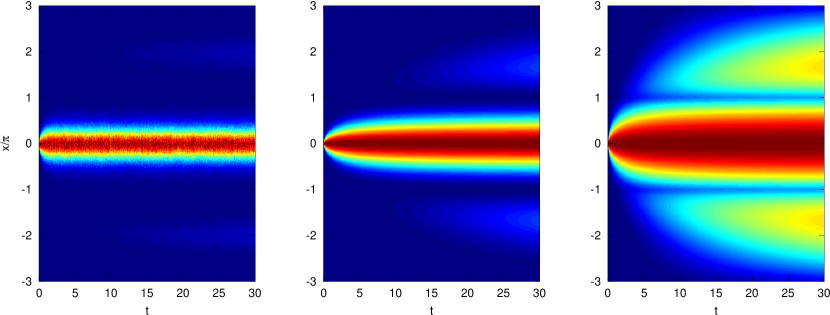
Figure 6: Weight function used for the PD example, (left) histogram of simulated paths used to fit the weight function, (centre) the weight function (10) with maximum likelihood parameter estimates $\epsilon=0.0259$ and $\sigma^{2}=0.3238$, and (right) the same weight function taken to the power 0.25 (used in the experiments). In all three cases the colour scheme is scaled between zero and the greatest value in each vertical section.

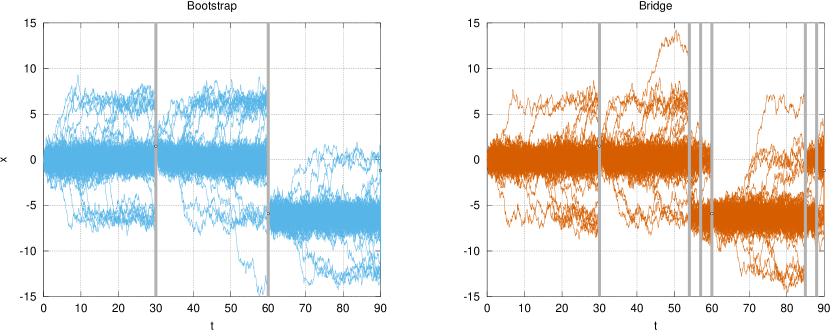
Figure 7: Diffusion bridge samples for the PD example with the data set of Lin et al. (2010), $x(0)=0,\,x(30)=1.49,\,x(60)=-5.91,\,x(90)=-1.17$, using a (left) bootstrap particle filter, and (right) bridge particle filter. Solid vertical lines indicate times at which resampling is triggered.

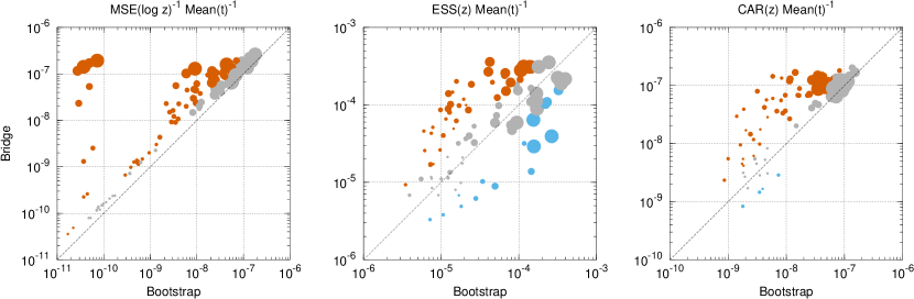
Figure 8: Metrics for the PD example, comparing the bootstrap and bridge particle filters. See Figure 2 caption for explanation.

4.4 Epidemiological SIR model

Consider an SIR (susceptible/infectious/recovered) model of an epidemic (Kermack and McKendrick, 1927), where $S(t)$ gives the number of susceptible individuals in a population over time, $I(t)$ the number of infectious individuals, and $R(t)$ the number of recovered individuals, parameterised by an infection rate $\beta$ and recovery rate $\nu$:

$$\frac{dS(t)}{dt} = -\beta S(t)I(t)$$

$$\frac{dI(t)}{dt} = \beta S(t)I(t)-\nu I(t)$$

$$\frac{dR(t)}{dt} = \nu I(t).$$

We introduce stochasticity into the system by allowing the original parameters $\beta$ and $\nu$ to vary in time (Liu and Stechlinski, 2012; Dureau et al., 2013), following the Itô SDEs:

$$dS(t) = -\beta(t)S(t)I(t)\,dt$$

$$dI(t) = \left(\beta(t)S(t)I(t)-\nu(t)I(t)\right)\,dt$$

$$dR(t) = \nu(t)I(t)\,dt$$

$$d\log\beta(t) = \left(\theta_{\beta,1}-\theta_{\beta,2}\log\beta(t)\right)\,dt+\theta_{\beta,3}\,dW_{\beta}(t)$$

$$d\log\nu(t) = \left(\theta_{\nu,1}-\theta_{\nu,2}\log\nu(t)\right)\,dt+\theta_{\nu,3}\,dW_{\nu}(t).$$

Note that $dS(t)+dI(t)+dR(t)=0$, so that total population is conserved, and that $\beta(t)$ and $\nu(t)$ are always positive. For numerical simulation, the SDEs are converted to ODEs with a discrete-time noise innovation:

$$\frac{dS(t)}{dt} = -\beta(t)S(t)I(t)$$

$$\frac{dI(t)}{dt} = \beta(t)S(t)I(t)-\nu(t)I(t)$$

$$\frac{dR(t)}{dt} = \nu(t)I(t)$$

$$\frac{d\log\beta(t)}{dt} = \theta_{\beta,1}-\theta_{\beta,2}\log\beta(t)+\theta_{\beta,3}\frac{\Delta W_{\beta}}{\Delta t}$$

$$\frac{d\log\nu(t)}{dt} = \theta_{\nu,1}-\theta_{\nu,2}\log\nu(t)+\theta_{\nu,3}\frac{\Delta W_{\nu}}{\Delta t}.$$

where each noise term $\Delta W\sim\mathcal{N}(0,\Delta t)$ is an increment of the Wiener process over a time step of size $\Delta t$. These ODEs are then numerically integrated forward using a low-storage fourth-order Runge–Kutta, with embedded third-order solution for error control, denoted RK4(3)5[2R+]C (Carpenter and Kennedy, 1994).

For the purposes of sampling diffusion bridges from the model, we wish to establish an $\epsilon$-ball around observations within which samples must fall, where $\epsilon$ is comparable to the discretisation error in simulating the model forward. It will make matters unnecessarily difficult to attempt to be any more accurate than this. The RK4(3)5[2R+]C algorithm outputs an error estimate for each variable at each time step, denoted $\epsilon_{S}(t)$, $\epsilon_{I}(t)$ and $\epsilon_{R}(t)$, computed as the difference between its third and fourth order solutions. A decison must then be made, according to these errors, whether to accept or reject the step. The particular implementation (Murray, 2012) in LibBi is based on the description of error control for the DOPRI5 method in Hairer et al. (1993). It uses an error tolerance parameterised by $\delta_{\text{abs}}$ (an absolute tolerance) and $\delta_{\text{rel}}$ (a relative tolerance). We set $\delta_{\text{abs}}=10^{-2}$ and $\delta_{\text{rel}}=10^{-5}$. For $X=\{S,I,R\}$, these are used to scale the error

$$\frac{\epsilon_{X}(t)}{\delta_{\text{abs}}+\delta_{\text{rel}}\left|X(t)\right|}.$$ (11)

The mean of these scaled errors is required to be less than one for the step to be accepted. If the step is rejected, the step size is reduced for a new attempt.

We suggest that it is sensible to use an $\epsilon$-interval on each observed variable that is commensurate with this discretisation error. We also note that the error estimate is of the local error of a single step of the numerical integrator, not of the cumulative error, which will be greater. We should therefore consider this estimate conservative, and may choose to inflate $\epsilon$ accordingly.

Only $I$ is observed in the data set used below. We introduce an indirect (albeit highly informative) observation $Y_{I}(t)$, with uniform observation model:

$$Y_{I}(t)\sim\mathcal{U}\left(I(t)-\epsilon(t),I(t)+\epsilon(t)\right).$$

We can set $\epsilon(t)=\delta_{\text{abs}}+\delta_{\text{rel}}\left|I(t)\right|$, using the same error threshold as in (11), but this leads to the peculiar situation where the interval is wider for larger $I(t)$, so that the model grants higher likelihood to smaller $I(t)$. This seems undesirable, so we remove the relative component. The overall population in the data set to be used is 763, so that the maximum error threshold is $\delta_{\text{abs}}+\delta_{\text{rel}}\times 763=0.01763$. Rounding up, we choose to set a constant $\epsilon=0.02$ for all $t$. With this in place, the errors in the observation, like those in numerical integration, are kept accurate to a small fraction of an individual of the population. We do not claim that this selection of $\epsilon$ is optimal, only that anything much less is futile without also tightening the error tolerances on the numerical integrator.

An alternative interpretation of this is as an ABC rejection algorithm with distance function $\rho(x(t),y(t)):=\left|I(t)-Y_{I}(t)\right|$ and acceptance criterion $\rho(x(t),y(t))\leq\epsilon$, with the choice of $\epsilon$ guided by the discretisation error of the numerical integrator.

We use Algorithm 3 with weight functions derived from the Gaussian process approach described in §3. The variance of the additional observation noise is set to $\varsigma^{2}(t)=\epsilon^{2}$. The data set records an outbreak of Russian influenza in a boys boarding school in northern England in 1978 (Anonymous, 1978). The data set is also studied in Ross et al. (2009).

We put prior distributions over the parameters:

$$\theta_{\beta,1} \sim \mathcal{U}(-100,100)$$

$$\theta_{\beta,2} \sim \Gamma(2,1)$$

$$\theta_{\beta,3} \sim \mathcal{U}(0,100)$$

$$\theta_{\nu,1} \sim \mathcal{U}(-100,100)$$

$$\theta_{\nu,2} \sim \Gamma(2,1)$$

$$\theta_{\nu,3} \sim \mathcal{U}(0,100),$$

and the initial values of state variables:

$$S(0) = 763-Y_{I}(0)$$

$$I(0) = Y_{I}(0)$$

$$R(0) = 0$$

$$\log\beta(0) \sim \mathcal{N}\left(\frac{\theta_{1,\beta}}{\theta_{2,\beta}},\frac{\theta_{3,\beta}^{2}}{2\theta_{2,\beta}}\right)$$

$$\log\nu(0) \sim \mathcal{N}\left(\frac{\theta_{1,\nu}}{\theta_{2,\nu}},\frac{\theta_{3,\nu}^{2}}{2\theta_{2,\nu}}\right).$$

Note that for $\log\beta(0)$ and $\log\nu(0)$, the prior is the same as the stationary distribution.

In preliminary experiments, we find that the bootstrap particle filter degenerates frequently for many settings of the parameters, while the bridge particle filter is much more reliable. Consequently, a PMMH chain using the bridge particle filter is configured as in Table 1 and used for a pilot run. This pilot run is continued until it appears to have converged to the posterior distribution, and has drawn enough samples to fit an improved random-walk Gaussian proposal. Initialised from the last state of the pilot run, we find that the bootstrap particle filter can now work more reliably and so may be used for a comparison. We run two chains, one using the bootstrap and the other the bridge particle filter, both initialised from the last state of the pilot run, and configured as in Table 1. Their resulting acceptance rates and effective sample sizes are reported there also. The chain using the bridge particle filter clearly performs better, although is slower also, given the additional resampling steps. The posterior results from this chain are given in Figure 9.

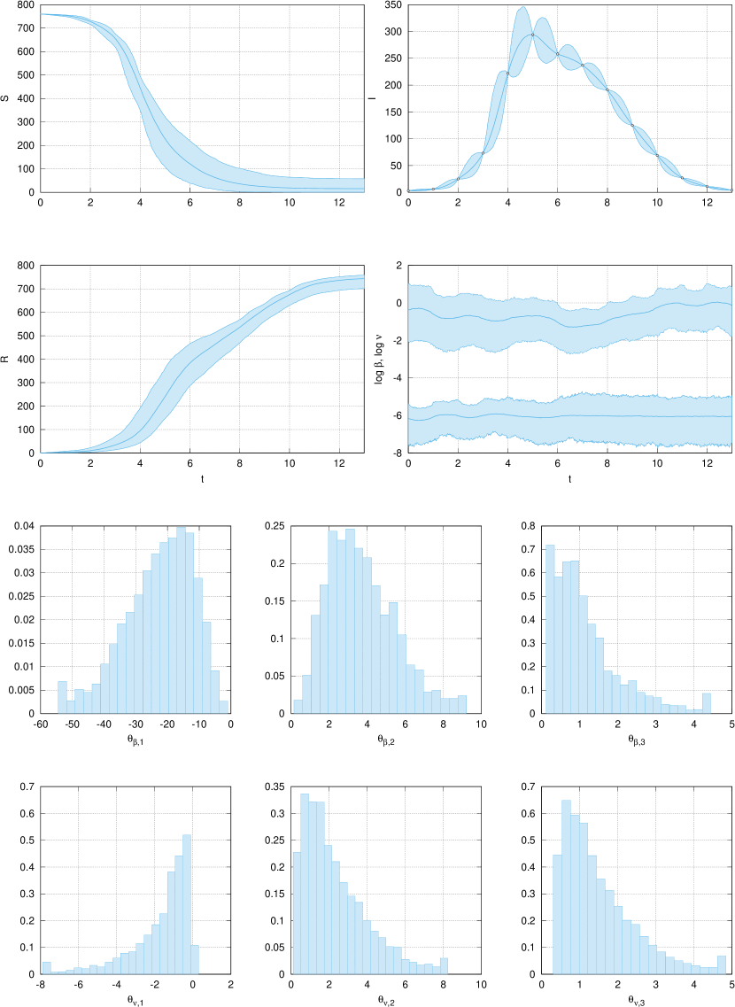
Figure 9: Posterior distributions over state variables and parameters for the SIR example, obtained with PMMH using the bridge particle filter. For state variables, shaded regions indicate 95% credibility intervals at each time, and middle lines the medians. Only $I$ is observed, with observations marked. For parameters, a normalised histogram is given.

4.5 Marine biogeochemical NPZD model

Marine biogeochemical models are an important means of assessing ecosystem health, especially in coastal environments. We adopt the NPZD model of Parslow et al. (2013). The model is described in detail in that work, and summarised in Murray et al. (2013). As even the summary takes some pages, we give only the high level motivation here.

An NPZD model represents the interaction of nutrients ($N$), phytoplankton ($P$), zooplankton ($Z$) and detritus ($D$) in a body of water. Each variable represents a compartment of a closed system, its value representing the quantity of nitrogen contained in that compartment. The four variables interact via a differential system where

$$\frac{dN(t)}{dt}+\frac{dP(t)}{dt}+\frac{dZ(t)}{dt}+\frac{dD(t)}{dt}=0,$$

such that the total quantity of nitrogen (in a closed system) is conserved. The fluxes between compartments are nonlinear functions of nine stochastic autoregressive terms, which model various biological, chemical and physical processes on a discrete-time daily time step. A basic loop is the absorption of nutrient by phytoplankton during growth, the grazing of phytoplankton by zooplankton, the death of zooplankton to produce detritus, and the remineralization of that detritus into nutrient. The fluxes between variables are not limited to these particular interactions, however.

The NPZD model is physically positioned somewhere in the open ocean, within the surface mixed layer. There, it is subjected to exogenous environmental forcings such as daily temperature and light availability, and is opened by a bottom boundary condition that permits a flux of nutrient from below.

The data set used is from the site of Ocean Station P in the north Pacific. This data set has been studied before in Matear (1995) and Parslow et al. (2013). We take four years of data, 1971–1974, as in Parslow et al. (2013). Observations include dissolved inorganic nitrogen ($Y_{N}$), considered an observation of nutrient ($N$), and chlorophyll-a fluorescence ($Y_{Chla}$), an observation of chlorophyll-a ($Chla$), itself a state variable that is a function of phytoplankton ($P$) and available light.

The observation model is:

$$\log Y_{N}(t) \sim \mathcal{N}(\log N(t),0.2)$$

$$\log Y_{Chla}(t) \sim \mathcal{N}(\log Chla(t),0.5).$$

While this observation model may appear only weakly informative, it can become highly informative given the sparsity (in time) at which observations are available. While the state variables tend to vary on daily or weekly time scales, the largest gap in observations of $Y_{N}$ is 136 days, and that of $Y_{Chla}$ 101 days.

We use Algorithm 3, with weight functions derived from the Gaussian process approach described in §3. Gaussian processes are fit to the logarithm of the observed time series of $Y_{N}$ and $Y_{Chla}$.

The first comparison is of the normalising constant estimates of the bootstrap and bridge particle filters, using the three metrics introduced above. We simulate 16 parameter sets from the prior distribution. The number of particles is set variously to $N\in\{2^{5},2^{6},\ldots,2^{10}\}$. Each unique pair of a parameter set and an $N$ constitutes an experiment, for 96 experiments in total. The bootstrap and bridge particle filters are applied to each experiment 1024 times, each time producing an estimate of the normalising constant. Each of the three metrics is computed from these estimates, for 288 comparisons in total. For computing the MSE-based metric, a bootstrap particle filter using $N=2^{20}$ is used to compute the “exact” log-likelihood for each parameter set. Results are in Figure 10.

The second comparison is to perform parameter estimation using a PMMH sampler. Two Markov chains are initialised from the same initial state, obtained from a pilot run that is assessed to have converged to the posterior distribution. The same proposal distribution is used for both chains. They are otherwise configured as in Table 1, where their acceptance rates and effective sample sizes are also reported. The posterior distribution for the chain using the bridge particle filter is given in Figure 11.

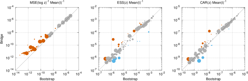
Figure 10: Metrics for the NPZD example, comparing the bootstrap and bridge particle filters. See Figure 2 caption for explanation.

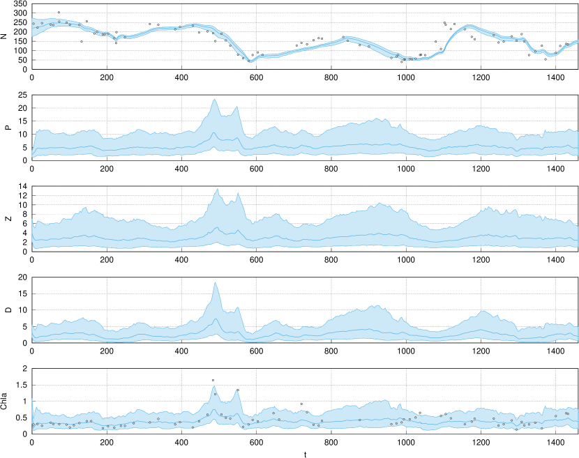
Figure 11: Posterior distributions over state variables for the NPZD example, obtained with PMMH using the bridge particle filter. Shaded regions indicate 95% credibility intervals at each time, and middle lines the medians. Both $N$ and $Chla$ are observed, with observations marked; others are unobserved.

5 Discussion

Of the four examples where the bootstrap and bridge particle filters are compared on metrics (OU, FFR, PD, NPZD), the bridge particle filter is consistently superior on the MSE metric, and at least as good on the ESS and CAR metrics. ESS is much better on the OU example, but similar on the others. CAR is much better on the OU example, modestly better on the FFR and PD examples, and similar on the NPZD example. This is evident in Figures 2, 4, 8 & 10. Recall that these metrics are already adjusted for execution time, which is typically longer for the bridge particle filter due to additional weighting and resampling steps.

Of the three examples where a comparison of PMMH performance using a real data set was attempted (FFR, SIR and NPZD), we were unable to find a working configuration for the bootstrap particle filter for the FFR example, and had difficulties configuring it for the SIR example due to frequent degeneracy. The bridge particle filter worked reliably in both cases, however. On the SIR and NPZD examples, the bridge particle filter outperforms the bootstrap on both ESS and acceptance rate (see Table 1). This suggests that the bridge particle filter can work well in cases where the bootstrap particle filter does not.

We can report that the process of pilot runs—for tuning the number of particles and proposal distribution—was less unpleasant than usual when using the bridge particle filter. For the SIR example, the bootstrap particle filter could not be made to work for such pilot runs, so that the bridge particle filter was required for this purpose. While anecdotal, this experience does affirm that the additional weighting and resampling steps are useful, and may compensate for a poor setting of parameters, or poorly fitting model.

There are a number of areas where care is needed in configuring the bridge particle filter:

1. The additional resampling steps can decrease performance, by introducing additional variance in the normalising constant estimate. The use of an adaptive resampling trigger (such as the ESS used here) mitigates this. In the empirical results of this work, the additional resampling steps appear to have a net benefit, or in the worst cases, do no harm.

2. The weight functions used may be too tight, so that particles are selected too aggressively at intermediate resamplings. For the PD, SIR and NPZD examples we have taken the weight function to the power 1/4 as a precaution. This seems sufficient for the examples here, but a more rigorous approach might be to use heavier-tailed weight functions (e.g. a Student $t$).

Finally, we have used a schedule of equispaced times for the additional weighting and resampling steps. This may be wasteful of compute resources. Alternative schedules may be superior, such as a geometric series of decreasing interval length, so that resampling is more frequent on approach to the observation. The schedule may even be adapted. We have found these ideas unecessary to pursue for the examples here, however, and so leave them to future work.

6 Conclusion

This paper has presented three related SMC methods for handling state-space models with highly-informative observations, including the special case of sampling bridges between fixed initial and final values. We have referred to them collectively as bridge particle filters. These bridge particle filters appear to improve substantially on the bootstrap particle filter in terms of the MSE of normalising constant estimates, and more modestly on other metrics. For two applications, we have been able to apply a PMMH sampler using bridge particle filters when we either could not do so, or had difficulty doing so, with a bootstrap particle filter, and we report anecdotally that these methods are quite straightforward to configure.

Supplementary material

All examples are available for download from the LibBi website (www.libbi.org).

References

- Andrieu et al. (2010) C. Andrieu, A. Doucet, and R. Holenstein. Particle Markov chain Monte Carlo methods. Journal of the Royal Statistical Society B, 72:269–302, 2010. doi: 10.1111/j.1467-9868.2009.00736.x.
- Anonymous (1978) Anonymous. Influenza in a boarding school. British Medical Journal, 1:587, March 1978. URL http://www.ncbi.nlm.nih.gov/pmc/articles/PMC1603269/?page=2.
- Aït-Sahalia (1999) Y. Aït-Sahalia. Transition densities for interest rate and other nonlinear diffusions. The Journal of Finance, 54(4):1361–1395, 1999. ISSN 1540-6261. doi: 10.1111/0022-1082.00149.
- Bayer and Schoenmakers (2013) C. Bayer and J. Schoenmakers. Simulation of forward-reverse stochastic representations for conditional diffusions. 2013. URL http://arxiv.org/abs/1306.2452.
- Beaumont et al. (2002) M. A. Beaumont, W. Zhang, and D. J. Balding. Approximate Bayesian computation in population genetics. Genetics, 162:2025–2035, 2002.
- Beaumont et al. (2009) M. A. Beaumont, J.-M. Cornuet, J.-M. Marin, and C. P. Robert. Adaptive approximate Bayesian computation. Biometrika, 96(4):983–990, 2009. doi: 10.1093/biomet/asp052.
- Beskos et al. (2006) A. Beskos, O. Papaspiliopoulos, G. Roberts, and P. Fearnhead. Exact and computationally efficient likelihood-based estimation for discretely observed diffusion processes. Journal of the Royal Statistical Society B, 68:333–382, 2006. doi: 10.1111/j.1467-9868.2006.00552.x.
- Carpenter and Kennedy (1994) M. H. Carpenter and C. A. Kennedy. Fourth-order 2N-storage Runge–Kutta schemes. Technical Report Technical Memorandum 109112, National Aeronautics and Space Administration, June 1994.
- Chopin et al. (2013) N. Chopin, P. Jacob, and O. Papaspiliopoulos. SMC2: An efficient algorithm for sequential analysis of state space models. Journal of the Royal Statistical Society B, 75:397–426, 2013. doi: 10.1111/j.1467-9868.2012.01046.x.
- Clark (1990) J. Clark. The simulation of pinned diffusions. In Proceedings of the 29th IEEE Conference on Decision and Control, pages 1418–1420. IEEE, 1990.
- Del Moral (2004) P. Del Moral. Feynman-Kac Formulae: Genealogical and Interacting Particle Systems with Applications. Springer–Verlag, 2004.
- Del Moral and Garnier (2005) P. Del Moral and J. Garnier. Genealogical particle analysis of rare events. The Annals of Applied Probability, 15(4):2496–2534, 11 2005. doi: 10.1214/105051605000000566.
- Del Moral et al. (2012) P. Del Moral, A. Doucet, and A. Jasra. An adaptive sequential Monte Carlo method for approximate Bayesian computation. Statistics and Computing, 22:1009–1020, 2012. doi: 10.1007/s11222-011-9271-y.
- Delyon and Hu (2006) B. Delyon and Y. Hu. Simulation of conditioned diffusion and application to parameter estimation. Stochastic Processes and their Applications, 116(11):1660 – 1675, 2006. ISSN 0304-4149. doi: 10.1016/j.spa.2006.04.004.
- Dureau et al. (2013) J. Dureau, K. Kalogeropoulos, and M. Baguelin. Capturing the time-varying drivers of an epidemic using stochastic dynamical systems. Biostatistics, 14(3):541–555, 2013. doi: 10.1093/biostatistics/kxs052.
- Durham and Gallant (2002) G. B. Durham and A. R. Gallant. Numerical techniques for maximum likelihood estimation of continuous-time diffusion processes. Journal of Business and Economic Statistics, 20(3):297–316, 2002.
- Elerian et al. (2001) O. Elerian, S. Chib, and N. Shephard. Likelihood inference for discretely observed nonlinear diffusions. Econometrica, 69(4):959–993, 2001. ISSN 00129682.
- Eraker (2001) B. Eraker. MCMC analysis of diffusion models with application to finance. Journal of Business & Economic Statistics, 19(2):177–191, 2001. doi: 10.1198/073500101316970403.
- Fearnhead et al. (2008) P. Fearnhead, O. Papaspiliopoulos, and G. O. Roberts. Particle filters for partially observed diffusions. Journal of the Royal Statistical Society B, 70:755–777, 2008. doi: 10.1111/j.1467-9868.2008.00661.x.
- Fearnhead et al. (2010) P. Fearnhead, O. Papaspiliopoulos, G. O. Roberts, and A. Stuart. Random-weight particle filtering of continuous time processes. Journal of the Royal Statistical Society B, 72(4):497–512, 2010. doi: 10.1111/j.1467-9868.2010.00744.x.
- Golightly and Wilkinson (2006) A. Golightly and D. J. Wilkinson. Bayesian sequential inference for nonlinear multivariate diffusions. Statistics and Computing, 16:323–338, 2006. doi: 10.1007/s11222-006-9392-x.
- Hairer et al. (1993) E. Hairer, S. Nørsett, and G. Wanner. Solving Ordinary Differential Equations I: Nonstiff Problems. Springer–Verlag, 2 edition, 1993.
- Kass et al. (1998) R. E. Kass, B. P. Carlin, A. Gelman, and R. M. Neal. Markov chain Monte Carlo in practice: A roundtable discussion. The American Statistician, 52(2):93–100, 1998. ISSN 00031305.
- Kermack and McKendrick (1927) W. O. Kermack and A. G. McKendrick. A contribution to the mathematical theory of epidemics. Proceedings of the Royal Society of London A: Mathematical, Physical and Engineering Sciences, 115(772):700–721, 1927. ISSN 0950-1207. doi: 10.1098/rspa.1927.0118.
- Kloeden and Platen (1992) P. E. Kloeden and E. Platen. Numerical Solution of Stochastic Differential Equations. Springer–Verlag, 1992.
- Lee (2008) A. Lee. Towards smooth particle filters for likelihood estimation with multivariate latent variables. Master’s thesis, University of British Columbia, 2008.
- Lin et al. (2010) M. Lin, R. Chen, and P. Mykland. On generating Monte Carlo samples of continuous diffusion bridges. Journal of the American Statistical Association, 105(490):820–838, 2010. doi: 10.1198/jasa.2010.tm09057.
- Lin et al. (2013) M. Lin, R. Chen, and J. S. Liu. Lookahead strategies for sequential Monte Carlo. Statistical Science, 28(1):69–94, 2013.
- Liu and Chen (1995) J. S. Liu and R. Chen. Blind deconvolution via sequential imputations. Journal of the American Statistical Association, 90:567–576, 1995.
- Liu and Stechlinski (2012) X. Liu and P. Stechlinski. Infectious disease models with time-varying parameters and general nonlinear incidence rate. Applied Mathematical Modelling, 36(5):1974–1994, 2012. ISSN 0307-904X. doi: 10.1016/j.apm.2011.08.019.
- Matear (1995) R. J. Matear. Parameter optimization and analysis of ecosystem models using simulated annealing: A case study at station P. Journal of Marine Research, 53(4):571–607, 1995. doi: 10.1357/0022240953213098.
- Murray (2012) L. M. Murray. GPU acceleration of Runge–Kutta integrators. IEEE Transactions on Parallel and Distributed Systems, 23:94–101, 2012. doi: 10.1109/TPDS.2011.61.
- Murray (2013) L. M. Murray. Bayesian state-space modelling on high-performance hardware using LibBi. In review, 2013. URL http://arxiv.org/abs/1306.3277.
- Murray et al. (2013) L. M. Murray, E. M. Jones, and J. Parslow. On disturbance state-space models and the particle marginal Metropolis–Hastings sampler. SIAM/ASA Journal of Uncertainty Quantification, 1(1):494–521, 2013. doi: 10.1137/130915376.
- Parslow et al. (2013) J. Parslow, N. Cressie, E. P. Campbell, E. Jones, and L. M. Murray. Bayesian learning and predictability in a stochastic nonlinear dynamical model. Ecological Applications, 23(4):679–698, 2013. doi: 10.1890/12-0312.1.
- Pedersen (1995) A. Pedersen. A new approach to maximum likelihood estimation for stochastic differential equations based on discrete observations. Scandinavian Journal of Statistics, 22(1):55–71, 1995.
- Peters et al. (2012) G. W. Peters, Y. Fan, and S. A. Sisson. On sequential Monte Carlo, partial rejection control and approximate Bayesian computation. Statistics and Computing, 22(6):1209–1222, 2012.
- Pitt and Shephard (1999) M. Pitt and N. Shephard. Filtering via simulation: Auxiliary particle filters. Journal of the American Statistical Association, 94:590–599, 1999.
- Pitt (2002) M. K. Pitt. Smooth particle filters for likelihood evaluation and maximisation. Technical Report 651, The University of Warwick, Department of Economics, July 2002.
- Roberts and Stramer (2001) G. O. Roberts and O. Stramer. On inference for partially observed nonlinear diffusion models using the Metropolis–Hastings algorithm. Biometrika, 88(3):603–621, 2001. doi: 10.1093/biomet/88.3.603.
- Ross et al. (2009) J. V. Ross, D. E. Pagendam, and P. K. Pollett. On parameter estimation in population models II: Multi-dimensional processes and transient dynamics. Theoretical Population Biology, 75:123–132, 2009.
- Schauer et al. (2013) M. Schauer, F. van der Meulen, and H. van Zanten. Guided proposals for simulating multi-dimensional diffusion bridges. 2013. URL http://arxiv.org/abs/1311.3606.
- Sisson et al. (2007) S. A. Sisson, Y. Fan, and M. M. Tanaka. Sequential Monte Carlo without likelihoods. Proceedings of the National Academy of Sciences, 104(6):1760–1765, 2007. doi: 10.1073/pnas.0607208104.
- Sun et al. (2013) L. Sun, C. Lee, and J. A. Hoeting. Penalized importance sampling for parameter estimation in stochastic differential equations. 2013. URL http://arxiv.org/abs/1305.4390.
- Van Kampen (2007) N. G. Van Kampen. Stochastic Processes in Physics and Chemistry. North Holland, 2007.