Self-referencing cellular automata: A model of the evolution of information control in biological systems

Abstract

Cellular automata have been useful artificial models for exploring how relatively simple rules combined with spatial memory can give rise to complex emergent patterns. Moreover, studying the dynamics of how rules emerge under artificial selection for function has recently become a powerful tool for understanding how evolution can innovate within its genetic rule space. However, conventional cellular automata lack the kind of state feedback that is surely present in natural evolving systems. Each new generation of a population leaves an indelible mark on its environment and thus affects the selective pressures that shape future generations of that population. To model this phenomenon, we have augmented traditional cellular automata with state/dependent feedback. Rather than generating automata executions from an initial condition and a static rule, we introduce mappings which generate iteration rules from the cellular automaton itself. We show that these new automata contain disconnected regions which locally act like conventional automata, thus encapsulating multiple functions into one structure. Consequently, we have provided a new model for processes like cell differentiation. Finally, by studying the size of these regions, we provide additional evidence that the dynamics of self/reference may be critical to understanding the evolution of natural language. In particular, the rules of elementary cellular automata appear to be distributed in the same way as words in the corpus of a natural language.

Introduction

Cellular automata (CA) are model complex systems that combine spatial memory with relatively simple update rules to produce rich dynamic patterns (Wolfram,, 2002). In this regard, they can be viewed as models for life. “Rules” in DNA encode policies that iteratively react to the environment by modifying it. Thus, over evolutionary time scales, natural selection can explore the nucleic/acid rule space and amplify those rules which provide useful functions. With this narrative in mind, researchers have used in silico artificial selection to explore the CA rule space and amplify rules with certain computational abilities (Das et al.,, 1994; Mitchell et al.,, 1994; Breukelaar and Bäck,, 2005; Hordijk,, 2013). Moreover, there has been much interest in understanding the demographic dynamics of these CA rule populations over their evolutionary history (Mitchell et al.,, 1994; Hordijk,, 2013). That is, artificial selection of these evolving CA’s has itself become a model for the innovation intrinsic to natural selection.

One major difference between evolving cellular automata (EvCA) and evolving natural organisms is the lack of feedback in the fitness channel of the former. In EvCA, each new generation faces the same selective pressures as prior generations. However, with new generations of natural organisms, there is feedback between the current demographics and the selective pressures shaping future demographics. Goldenfeld and Woese, (2011) point out that these self/referential dynamics are a unique characteristic of life – making life distinctly different from any other physical system. Two of us (SIW and PCWD) have proposed that self/referential dynamics are one of the hallmarks of life, emerging with its origin (Walker and Davies,, 2013). Where EvCA’s will only innovate in the presence of external “abiotic” pressures, natural organisms put pressure on themselves to re/organize even without an external fitness driver. Similarly, at everyday and ontogenetic time scales, conventional CA’s do not easily embed the regulatory mechanisms that permeate throughout life. A single genome gives rise to a wide variety of differentiated cell phenotypes which, locally, appear to follow a consistent set of operational rules but globally appear to have no shared program. By modeling feedback explicitly, these phenomena can be explained using gene regulatory network (GRN) frameworks (Schlitt and Brazma,, 2007; Davidson,, 2010), where the expression level of one gene promotes or inhibits the expression level of another and thus “latches” cells into different types. Thus, by making feedback between state and dynamics explicit in CA’s, it may be possible to enrich their ability to model how organisms emerge, evolve, develop, and react to both their external environment and their internal state.

Here, we introduce self/referencing cellular/automaton framework we call PICARD where PICARD Implements CA Rules Differently (PICARD). Like a traditional one/dimensional CA, PICARD executions move from one iteration to another by some rule. However, whereas traditional CA’s require the rule to be static and externally specified, PICARD infers the iteration rule from the current state of the CA itself. As we will show, executions from multiple static CA’s can be embedded within a single PICARD – a PICARD can be identical to one static CA from certain initial conditions and another static CA from other initial conditions. Thus, a PICARD can combine the computational abilities of different CA’s within one entity. Moreover, whereas CA’s differ by their rule, PICARD’s differ by their state-to-rule mapping. Because there are many more state-to-rule mappings than there are CA rules, the PICARD parameter space is potentially much richer for later evolutionary investigations.

To some extent, PICARD is a simple attempt to add dynamical feedback that is missing in traditional evolutionary cellular automata. However, because iterations are generated by rules that are encoded in previous iterations, PICARD feedback is the kind of self/reference that is thought to be a characteristic feature of life (Hofstadter,, 1979; Kataoka and Kaneko, 2000a, ; Kataoka and Kaneko, 2000b, ; Goldenfeld and Woese,, 2011; Walker and Davies,, 2013). Our CA approach shares many similarities with self/referencing functional/dynamics developed by Kataoka and Kaneko, 2000a to model the evolution of rules (Kataoka and Kaneko, 2000a, ; Kataoka and Kaneko, 2000b, ). Attempting to avoid the biochemical complexities of the evolution of nucleic acids, they turn their focus on the evolution of natural language. Furthermore, they draw connections between attractors in their coupled/logistic/map landscape and words that accumulate in language. Although their framework is very different than the automata we study here, we too have results that appear to be strongly connected to the evolution of natural language. Thus, augmenting cellular automata with self/reference widens our ability to model to evolution of language in unanticipated ways.

Cellular Automata with PICARD Mappings

Although PICARD implements CA rules differently, once each rule is defined, a PICARD iteration is identical to an iteration of a conventional elementary CA. As shown in Fig. 1(a), a traditional elementary CA generates each row based on the pattern in the preceding row.

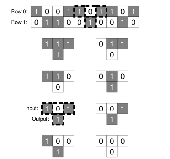
(a) Single iteration of rule 182

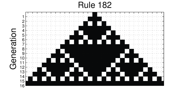
(b) Execution of rule 182

Figure 1: Traditional cellular automaton. In 1(a), a single iteration of a traditional CA is shown in the top two rows, where row 0 is taken as an initial condition on which a static CA rule operates to produce row 1. The static CA rule is summarized in the eight groups of four cells in the bottom of the figure. In each group, the top three cells match adjacent cells in row 0, and the bottom one cell represents the cell generated beneath the row-0 cells in row 1. One such grouping in the two rows is outlined in a broken line along with the corresponding group from the elementary CA rule below it. This CA rule can be equivalently summarized as an eight-bit binary string 0b10110110, a two/digit hexadecimal 0xB6, or a decimal 182. In 1(b), an execution of rule 182 is shown that resembles a Sierpinski triangle.

The iteration rule is a lookup table that maps each triplet of bits in the preceding row to a single bit in the following row. Thus, with the right initial conditions, some rules can produce intricate patterns over many generations, as shown in Fig. 1(b).

Where PICARD differs from a traditional CA is that no static rule is specified. Instead, a map is provided from each row to the rule that will operate on it. We are primarily interested in CA’s with more than eight cells; consequently, this mapping is a coarse graining of the system – some rules will necessarily correspond to multiple different row patterns. With this multiple realizability of rules in mind, each PICARD row and rule can be viewed as a microstate-macrostate pair. Consequently, in the following, we will use the terms rule and macrostate interchangeably.

For example, Fig. 2 shows two arbitrary examples of microstate/to/rule mappings.

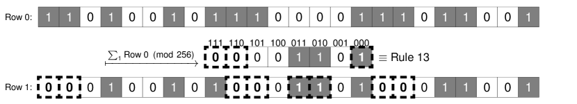
(a) Sum of ones

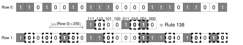
(b) Density of ones

Figure 2: Example aggregation PICARD mappings. The CA rule induced by each mapping is shown between rows 0 and 1, where the triplet above each position represents the pattern of bits in row 0 that will result in the boxed bit in row 1. Positions in the rule that result in a changed bit from row 0 to row 1 have been highlighted with broken lines; the resulting toggled bits in row 1 have also been highlighted. Each mapping represents some aggregate property of the first row. In 2(a), the rule represents the total number of 1’s in row 0, modulo 256. Because there are only 24 cells in the row, this PICARD mapping can only induce 25 different elementary CA rules. In the case of a row with more than 255 cells, every elementary rule is possible. In 2(b), the rule represents the density of 1’s in row 0 scaled by 255.

Each of these two mappings extract an aggregate property of the corresponding row. In Fig. 2(a), the focal macrostate is the number of 1’s in the row. In Fig. 2(b), the focal macrostate is the density of 1’s in the row. For the analogous case of interacting particles, macroscopic aggregates like temperature and pressure are not typically viewed as having causal influence on the microscopic states of the system. That is, macroscopic states and microscopic states exist in two different levels of description. However, if a collection of particles is put into contact with a heat bath characterized by only its temperature, the macroscopic properties of the gas appear to drive the evolution of the microscopic system. Likewise, these PICARD aggregation mappings are simultaneously descriptive coarse grainings as well as prescriptive rules governing the dynamics of the cells. Goldenfeld and Woese, (2011) argue that self/reference appears in biological systems but apparently not in physical systems because of similar reasoning – biological phenomena are emergent and may require self/reference for analysis without appealing to underlying interacting physical microstates. Self/reference therefore may be intimately related to framework suggested to characterize emergence, such as top-down causation (Davies,, 2012), and may play an important role in the emergence of new organizational levels through major evolutionary transitions (Walker et al.,, 2012).

Aggregation mappings may have intuitive connections to statistical mechanics, but PICARD mappings may be built in entirely different ways. The block mappings in Fig. 3 are formed by clustering bits of the CA microstate into eight groups and matching each group to a predicate function that determines the bit in the rule which has the same relative position as the 3-bit group.

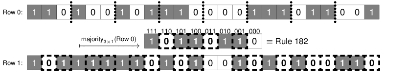
(a) Block ones majority

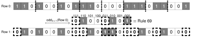
(b) Block ones odd parity

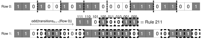
(c) Block transition odd parity

Figure 3: Example block PICARD mappings. Rules are shown just as in Fig. 2. However, the 24 bits in row 0 have been broken into 8 3-bit clusters shown with separating fences. The eight bits of the rule are then induced from a simple 3-bit predicate from each group to the corresponding rule bit. In 3(a), each bit in the rule is a 1 if and only if the corresponding 3-bit cluster in row 0 has a majority of 1’s. In 3(b), the rule bit is set if there are an odd number of 1’s in the cluster. In 3(c), the rule bit is set if there are an odd number of zero/to/one or one/to/zero transitions in the 3-bit cluster (see Table 1).

Microstate Block	Number of Transitions	Rule Bit
000	0	0
001	1	1
010	2	0
011	1	1
100	1	1
101	2	0
110	1	1
111	0	0

Table 1: Lookup table for transition odd parity. Reading from left to right, the number of zero/to/one and one/to/zero transitions is counted. The odd parity of this count is equivalent to the exclusive or of the outer two bits in the microstate block.

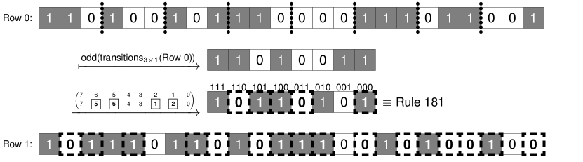
Figure 4: Block transition mapping with permutation. This PICARD mapping is equivalent to the mapping from Fig. 3(c) composed with a permutation that switches middle two bits of each nybble.

For example, in Fig. 3(a), the 24 bits of the microstate are broken into eight mutually exclusive groups of three bits. Each 3-bit group is replaced by a single 1 if it has a majority of 1’s and a 0 otherwise. In Fig. 3(b), groups are mapped into 1 if they have an odd number of 1’s. Alternatively, in Fig. 3(c), the actual binary identity of the bits in each group is ignored and instead the number of transitions is used (see Table 1). That is, from left to right within each 3-bit group, a cell will transition from one level to another 0, 1, or 2 times. The corresponding rule bit will be a zero unless the 3-bit group only contains a single transition. This predicate is equivalent to the exclusive or (XOR) of the outer two bits in the microstate group. As these examples show, PICARD executions starting from the same microstate can be very different based on the chosen mapping from microstate to rule.

While the predicates used within block mappings may be relatively simple, the selection of microstate and macrostate bits for each block mapping adds an additional layer of complexity. For example, a single PICARD block mapping may use different predicates for each microstate block. Additionally, microstate blocks may not be mutually exclusive – they may overlap or leave some microstate bits uncovered. Even when a a single predicate is used over a set of mutually exclusive, equally sized microstate groups that cover all microstate bits, the ordering of the microstate groups need not match the ordering of the corresponding rule bits. In Fig. 4, a mapping of this sort is shown. That is, the mapping from Fig. 3(c) has been composed with a permutation. For the remainder of this paper, we will use this mapping to demonstrate the richness of an individual PICARD.

A PICARD Case Study

In the following, we consider the mapping described above in Fig. 4. Because the rule induced by each row can be viewed as a macrostate of the system, it is useful to consider both the CA microstate dynamics and the rule macrostate dynamics. In Fig. 5, executions of the PICARD mapping are shown starting from three different initial conditions. The executions of the CA are shown in the left column, and the corresponding executions through the macrostate rule space is shown in the right column.

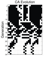
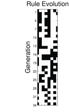
(a) Execution leading to mutual oscillation

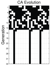
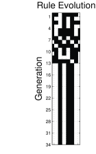
(b) Execution leading to mutual fixed points

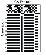
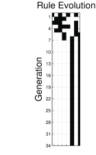
(c) Microstate oscillations under invariant rule

Figure 5: Example PICARD executions. Cellular automata on the left are adjacent to their corresponding rule histories on the right. Executions in 5(a) and 5(b) show CA and rule histories that have equilibria of the same type. In 5(c), an execution is shown where oscillations in microstate do not correspond to oscillations in rule.

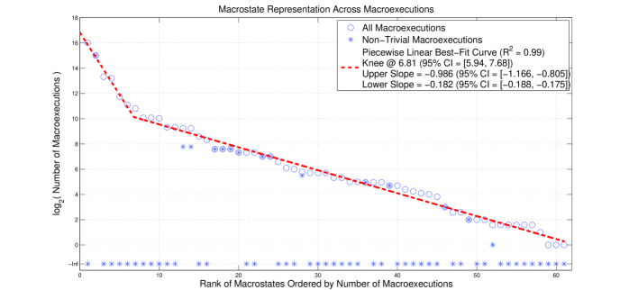
Figure 6: Macrostate representation over macroexecutions. Each macrostate may be invariant across a range of disconnected macroexecutions. Every macroexecution terminates in a fixed point or a periodic cycle of microstates that each correspond to the same macrostate. Each terminating fixed point or cycle may be reached from a number of other transient microstates which themselves correspond to that same macrostate. A complete macroexecution includes the terminating cycle and all leading transient microstates which share the same macrostate. Using the PICARD mapping from Fig. 4, the entire microstate space has been explored and every complete macroexecution has been found. Displayed here as open circles are the $\log_{2}$/scaled counts of macroexecutions within each macrostate, omitting macrostates with no macroexecutions. The asterisks represent the $\log_{2}$-scaled count of macroexecutions after all fixed/point macroexecutions are removed. The horizontal axis shows the rank of the corresponding macrostate when ordered by the total number of complete macroexecutions within it. A broken piecewise/linear line of best fit is shown with an upper slope near $-1$.

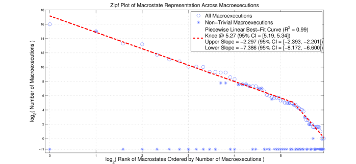
Figure 7: Zipf plot of macrostate distribution over macroexecutions. Displayed are the data from Fig. 6; however, the horizontal axis is also $\log_{2}$ scaled. The broken piecewise/linear line of best fit shows that the distribution is approximately Zipfian.

In general, the lower resolution macrostate executions are each visually similar to their higher resolution microstate. In Fig. 5(a), the microstate reaches a steady/state oscillation. Given that the rule that governs the microstate evolution is derived from the microstate itself, it is not surprising that the macrostate also reaches a steady/state oscillation. Similarly, in Fig. 5(b), the microstate and macrostate both reach a fixed point. However, while the CA does not reach its fixed point until generation 16, its macrostate becomes fixed in generation 14. Thus, at generation 14, this PICARD degenerates into an elementary CA under rule 44 (i.e., 0b00101100). If all generations before 14 were removed from the history of the CA, it would be indistinguishable from an elementary CA. Moreover, as shown in Fig. 5(c), this phenomenon is not restricted to only fixed points. By generation 8, the rule trajectory becomes fixed on rule 5 (i.e., 0b00000101); however, the CA trajectory reaches a steady/state oscillation where some cells are fixed and others cycle. Again, the tail of this CA execution is indistinguishable from one that would be generated under elementary CA rule 5. Consequently, this single PICARD mapping is able to represent executions from multiple elementary CA rules simultaneously while also potentially producing novel executions.

When a PICARD mapping generates an execution that is in a region of macrostate invariance, we call that execution a macroexecution. Once a macroexecution has been reached, state feedback is not required to determine the future trajectory. Thus, macroexecutions move through regions of locally elementary CA space. For the mapping explored in this section, Fig. 6 shows the relative “size” of each of these locally elementary regions. In particular, for each of the 256 elementary CA rules, all of the disconnected macroexecutions for which the rule is invariant were counted. The rules with non/zero counts were ranked and plotted as the open circles in the semilog frequency distribution in Fig. 6. The asterisks on the plot represent the number of oscillatory macroexecutions – that is, the asterisks represent the count when the fixed/point macroexecutions are removed. Thus, the highest ranking elementary CA rule includes all fixed/point macroexecutions, but the second ranking elementary CA rule includes no fixed/point macroexecutions.

As shown by the piecewise linear broken line in Fig. 6, the highest ranking elementary CA rules have counts which peak at $2^{16}$ and are halved with each increase in rank over a significant range of rules. However, this trend is not long lasting and may simply be an artifact of the particular PICARD mapping we have chosen for this case study. In Fig. 7, the same distribution is shown on a log–log plot and shows evidence that the greater trend is Zipfian (Zipf,, 1949). Words in a language tend to be Zipfian distributed in their use – the relative frequency of words is inversely proportional to their rank. Following an analogy with language, elementary CA rules act like words which are used in PICARD macroexecutions. Using a functional/dynamics framework as a model for the evolution of natural language, Kataoka and Kaneko, 2000b show how self/referencing function dynamics can act like a filter that produces a corpus of words that are each fixed points of the dynamical model. The invariant macrostate CA rules that we describe are qualitatively similar to this idea, and their representation is consistent with measured distributions of words in actual natural language.

The data from Fig. 6 have been reproduced in Table 2 for the sixteen highest/ranking macrostates.

Rule	Macroexecutions	Non/trivial Macroexecutions
204 (0xCC)	65536	0
51 (0x33)	32768	32768
205 (0xCD)	10196	0
76 (0x4C)	9360	0
236 (0xEC)	3420	0
200 (0xC8)	2166	0
4 (0x04)	1792	0
12 (0x0C)	1072	0
132 (0x84)	1072	0
68 (0x44)	1040	0
140 (0x8C)	640	0
196 (0xC4)	640	0
108 (0x6C)	603	219
201 (0xC9)	603	219
232 (0xE8)	384	0
77 (0x4D)	320	0

Table 2: Sixteen highest ranking macrostates.

.

The two highest/ranking macrostates, rule 204 and rule 51, each have a number of macroexecutions that is a power of two, $2^{16}$ and $2^{15}$. In the case of rule 204, its macroexecutions exhaust all of the $2^{16}$ microstates that map to it. Thus, rule 204 has no transients – it is a region filled entirely with fixed points. Likewise, because there are no fixed points in rule 51 and yet $2^{15}$ macroexecutions, each macroexecution must be a period/2 cycle. So the rule-51 region also has no transient microstates, but it is filled entirely with these cycles. Moving farther down the ranks, more microstates become available for forming macroexecutions with longer/period oscillations within them. For example, Fig. 8 shows a period/6 oscillation embedded within a rule-109 macroexecution.

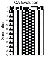
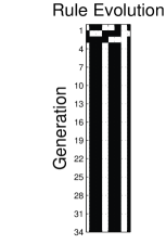
Figure 8: Period/6 macroexecution with short transient. A steady/state rule-109 (0x6D) macroexecution is shown that has a period of six generations preceded by its longest possible transient. Rule 109 has 31 macroexecutions, which are all non/trivial.

Because each of the $2^{8}$ macrostates represents a finite number of microstates ($2^{16}$), the upper bound on the number of distinct oscillations which are macrostate invariant must decrease with the average length of those oscillations. Likewise, rule 109 has only 31 macroexecutions, which are all non/trivial and thus all end on cycles of period 2 or greater. Although this mapping favors short/period oscillations, other mappings may allow for longer cycles. For example, if the aggregate sum mapping in Fig. 2(a) is composed with a function that maps a unity sum to rule 4, then PICARD will shift each sum-1 row to the right by one position on each iteration. These shifts will not alter the sum of the row, and thus this shifting will continue indefinitely. Consequently, in this hypothetical case, the rule-4 region will contain macroexecutions with periods as long as the length of each microstate row. However, by the discussion above, rule 4 is unlikely to contain a high number of macroexecutions due to the number of microstates consumed by these long/period oscillations.

As shown above in Fig. 5(a), PICARD oscillations need not be contained within a macroexecution – microstates can oscillate across rule boundaries. Additionally, the transient components of PICARD executions can have rich structure. In Fig. 9, there is a long sequence of transient execution leading up to an eventual rule-0 fixed point.

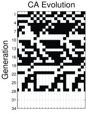
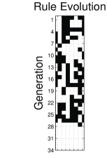
Figure 9: Fixed point with long structured transient. A rule-0 fixed point is shown that is preceded by a very long transient that appears to have significant visual structure.

The CA appears to have significant structure visually, but the rule evolution is less predictable and shows clear path dependence. Thus, the feedback in PICARD both constrains its executions and generates novel patterns that may be fodder for further analysis.

Summary and Future Work

By feeding a conventional one/dimensional elementary cellular automaton’s own state back into the iteration rule that generates its next state, we have developed a new modeling framework for investigating information control in natural systems. Although open/loop cellular automata that evolve under strictly static rules have been useful tools for studying evolution artificially, these classic frameworks are not sufficiently rich to model the dependence of fitness on current state. Moreover, by adapting the methods of evolving cellular automata so that PICARD mappings can be the targets of artificial selection, there is a potentially richer set of behaviors that can be selected for.

We have shown how state feedback can generate self/reinforcing regions of behavior. Thus, this framework provides a model of how functional diversity can be embedded within a single automaton. This functional diversity is similar to the diverse differentiation possibilities for cells in living organisms. Moreover, as evidenced by the distribution of macrostates over macroexecutions, this framework apparently shares similarities with the processes responsible for the generation of natural language.

A possible criticism of PICARD is that it introduces non/local effects to cellular automata. Traditional CA are built from the assumptions that cells update based entirely on local information and information about neighbors. By feeding the state of an entire row back into the CA rule, this locality assumption is broken. A complete reductionist model of the dynamics of life would necessarily have to incorporate dynamics of both the focal entity and the environment around it – despite any significant differences in time scales. By feeding the state of the focal entity back into the rules that govern how the entity evolves, we avoid these complications and still allow for entities to alter and be altered by their environment. Thus, just as coarse/grained descriptions have utility in modeling physical phenomena, non/local effects in PICARD mappings can be viewed as useful coarse/grainings of otherwise less tractable models.

As PICARD Implements CA Rules Differently, there are myriad directions for future work – including directions which parallel investigations from conventional cellular automata and directions which are specific to PICARD self/reference. At a minimum, the distribution of macrostates over macroexecutions needs to be investigated for a wide variety of PICARD mappings to determine whether the Zipfian distribution is widespread. Although it is attractive to view the PICARD automata in this paper as a mosaic of different elementary CA that each govern small patches of local elementarity, it is unlikely that such regions exist that contain executions with the relatively open/ended complexity of open/loop elementary CA patterns. However, PICARD mappings have the potential of generating new patterns and new functionality that may be out of reach of conventional CA’s. Alternatively, PICARD mappings may have the ability to increase the robustness of elementary CA function by reducing the sensitivity to minute but functionally inconsequential changes in initial condition. Extending PICARD mappings to be able to map from prior microstates may allow for incorporating functionality normally associated with higher/dimensional cellular automata. For example, Langton,’s loops (Langton,, 1984) are able to self replicate because growing patterns in space can turn and interact with earlier patterns. A PICARD mapping can similarly connect iterations across time and draw a connection between two/dimensional self replication and one/dimensional pattern generation. In general, an important future direction is to connect one/dimensional PICARD insights to higher dimensional cellular automata.

References

- Breukelaar and Bäck, (2005) Breukelaar, R. and Bäck, T. (2005). Using a genetic algorithm to evolve behavior in multi dimensional cellular automata: emergence of behavior. In Proceedings of the 7th Annual Conference on Genetic and Evolutionary Computation (GECCO ’05), pages 107–114, Washington, DC, USA.
- Das et al., (1994) Das, R., Mitchell, M., and Crutchfield, J. P. (1994). A genetic algorithm discovers particle computation in cellular automata. In Proceedings of the Third Conference on Parallel Problem Solving from Nature, volume 866 of Lecture Notes in Computer Science, pages 344–353. Springer.
- Davidson, (2010) Davidson, E. H. (2010). The Regulatory Genome: Gene Regulatory Networks In Development And Evolution. Academic Press.
- Davies, (2012) Davies, P. C. W. (2012). The epigenome and top-down causation. Interface Focus., 2(1):42–48.
- Goldenfeld and Woese, (2011) Goldenfeld, N. and Woese, C. (2011). Life is physics: evolution as a collective phenomenon far from equilibrium. Annu. Rev. Condens. Matter Phys., 2(1):375–399.
- Hofstadter, (1979) Hofstadter, D. R. (1979). Gödel, Escher, Bach: an Eternal Golden Braid. Basic Books, Inc.
- Hordijk, (2013) Hordijk, W. (2013). The EvCA project: a brief history. Complexity, 18(5):15–19.
- (8) Kataoka, N. and Kaneko, K. (2000a). Functional dynamics. I: articulation processes. Phys. D: Nonlinear Phenom., 138(3–4):225–250.
- (9) Kataoka, N. and Kaneko, K. (2000b). Natural language from function dynamics. Biosystems, 57(1):1–11.
- Langton, (1984) Langton, C. G. (1984). Self-reproduction in cellular automata. Phys. D: Nonlinear Phenom., 10(1–2):135–144.
- Mitchell et al., (1994) Mitchell, M., Crutchfield, J. P., and Hraber, P. T. (1994). Evolving cellular automata to perform computations: mechanisms and impediments. Phys. D: Nonlinear Phenom., 75(1–3):361–391.
- Schlitt and Brazma, (2007) Schlitt, T. and Brazma, A. (2007). Current approaches to gene regulatory network modelling. BMC Bioinformatics, 8(6).
- Walker et al., (2012) Walker, S. I., Cisneros, L., and Davies, P. C. W. (2012). Evolutionary transitions and top-down causation. In Proceedings of the Thirteenth International Conference on the Simulation and Synthesis of Living Systems (Artificial Life 13), volume 13, pages 283–290, East Lansing, Michigan.
- Walker and Davies, (2013) Walker, S. I. and Davies, P. C. W. (2013). The algorithmic origins of life. J. R. Soc. Interface, 10(79).
- Wolfram, (2002) Wolfram, S. (2002). A New Kind of Science. Wolfram Media.
- Zipf, (1949) Zipf, G. K. (1949). Human Behavior and the Principle of Least Effort. Addison-Wesley Press, Oxford, England.