Rayleigh-Taylor instability in Magnetohydrodynamic Simulations of the Crab Nebula

Abstract

In this paper we discuss the development of Rayleigh-Taylor filaments in axisymmetric simulations of Pulsar wind nebulae (PWN). High-resolution adaptive mesh refinement magnetohydrodynamic (MHD) simulations are used to resolve the non-linear evolution of the instability. The typical separation of filaments is mediated by the turbulent flow in the nebula and hierarchical growth of the filaments. The strong magnetic dissipation and field-randomization found in recent global three-dimensional simulations of PWN suggests that magnetic tension is not strong enough to suppress the growth of RT filaments, in agreement with the observations of prominent filaments in the Crab nebula. The long-term axisymmetric results presented here confirm this finding.

1 Introduction

The Crab Nebula is a product of the supernova explosion observed by Chinese and Arab astronomers in 1054. It belongs to the class of Pulsar Wind Nebulae (PWN), bubbles of non-thermal plasma inflated inside of expanding supernova ejecta by magnetized neutron stars produced during core-collapse stellar explosions. The spectacular network of line-emitting filaments of the Crab Nebula is one of its most remarkable features. In projection, these filaments appear to occupy more or less the same space as the more amorphous non-thermal optical and radio emission. Most individual filaments are small scale structures but some are much longer and appear to cross almost the entire nebula. Images obtained at different epochs reveal radial expansion of the filamentary network (Trimble, 1968). The speed of the proper motion of the filaments increases towards the outer edge. The line-of sight speeds, obtained via spectroscopic observations, show the opposite trend (Lawrence et al., 1995), thus confirming the overall radial expansion of the network. Moreover, the narrow band images of the Crab Nebula show that the filaments with low line-of-sight speed avoid the central part of the nebula image (Lawrence et al., 1995). This indicates that the Crab filaments do not penetrate the whole volume of the nebula, as otherwise low line-of-sight-speed emission would be seen there. Instead, the filaments reside near its outer edge, where they occupy a thick shell of thickness 0.3-0.7 pc, which is about one third of the nebula radius (Clark et al., 1983; Lawrence et al., 1995).

Initially, it was thought that the filaments could be the debris of the stellar envelope produced during the supernova explosion. However, this interpretation is in conflict with the low total mass of the filaments, $2-5M_{\sun}$ and their low speed, only $\leq 1500$ km/s, resulting in total energy of the explosion which is well below the typical one for core-collapse supernovae (Hester, 2008). In order to bring these values up towards the expectations, one has to assume that most of the supernova ejecta is not visible yet. Most probably, the ejecta size significantly exceeds that of the Crab nebula and remains invisible due to low density ISM and hence a weak forward shock, whereas the observed thermal emission of the nebula comes as a result of the interaction between the inner part of the ejecta and the relativistic wind of the Crab pulsar (Rees & Gunn, 1974; Kennel & Coroniti, 1984).

The high pressure of the hot bubble inflated by the pulsar wind inside of the ejecta drives a shock wave into the cold ejecta, heating its plasma and making it visible. Indeed, deep images of the Crab Nebula in high-ionization lines reveal a sharp outer edge, which can be identified with this shock (Gull & Fesen, 1982; Sankrit & Hester, 1997). The non-thermal emission is generally confined within this edge, in agreement with this interpretation, although the edge is not seen in it in the north-west part of the nebula, there the radio emission seems to extend beyond the thermal one (e.g. Velusamy, 1984). However, the cooling time of the post-shock gas and brightness of its emission is a strong function of the ejecta density and the observations may simply indicate lower ejecta density in the NW-direction (Sankrit & Hester, 1997).

The ejecta is much denser than the PWN bubble and provided the shock, and hence the contact discontinuity separating the shocked ejecta from the bubble, expands with increasing speed, this configuration is similar to the one where a heavy fluid is placed on top of a light one in gravitational field. The latter is known to be Rayleigh-Taylor (RT) unstable. During the non-linear phase of this instability, the heavy fluid forms fingers which stream downwards and the light fluid forms bubbles rising between the fingers. Chevalier & Gull (1975) proposed that this is the origin for the thermal filaments of the Crab Nebula. The possibility of acceleration is strongly supported by both the observations and the theoretical models of PWN. Indeed, the estimates of the nebula age based on its observed size and expansion speed are significantly shorter compared to that based on the time of the supernova explosion, implying accelerated expansion (e.g. Trimble, 1968; Bietenholz et al., 1991). Strengthening this conclusion, the self-similar model of PWN inflated inside the ejecta with density $\rho\propto r^{-\alpha}$ by a pulsar wind of constant power yields the shock speed

$$v_{sh}\propto t^{1/(5-\alpha)}$$ (1)

(Chevalier & Fransson, 1992).

The RT instability has been a subject of many theoretical studies. The original problem, involving ideal incompressible semi-infinite fluids in slab geometry, has been expanded to study the role of other factors, such as viscosity, surface tension, different geometry, magnetic field etc. For the original problem, the linear theory of the RT instability gives the growth rate

$$\omega^{2}=Agk\,,$$ (2)

where $g$ is the gravitational acceleration and $k$ is the wavenumber of the perturbation and where we introduce the Atwood number $A=(\rho_{2}-\rho_{1})/(\rho_{2}+\rho_{1})$, where $\rho_{1}$ and $\rho_{2}$ are the mass densities of light and heavy fluids respectively. Thus, smaller scale structures grow faster. The transition to the non-linear regime occurs when the amplitude of the interface distortion becomes comparable to the wavelength. At the onset of this phase, the light fluid forms bubbles/columns of diameter $\sim\lambda$ which steadily rise with the speed

$$v_{b}\simeq 0.5\sqrt{g\lambda}\,,$$ (3)

whereas the heavy fluid forms thin fingers approaching the state of free fall (e.g. Davies & Taylor, 1950; Frieman, 1954; Youngs, 1984; Kull, 1991; Ramaprabhu et al., 2012). Thus at this stage, bubbles of larger scales grow faster and eventually dominate the smaller ones. This has been observed both in laboratory and in simulations (e.g. Youngs, 1984; Jun, Norman & Stone, 1995; Stone & Gardiner, 2007). Interestingly, the initially dominating small scale perturbations appear to be washed out completely when much larger scales begin to dominate. Even if the initial spectrum of linear perturbations has a high wavelength cutoff, structures on the length scale exceeding it may appear via a kind of inverse cascade process, where smaller bubbles merge and create larger ones (Sharp, 1984; Youngs, 1984). The dynamics of bubbles and fingers is influenced by secondary Kelvin-Helmholtz instability, which facilitates transition to turbulence and mixing between the fluids. This could be the reason for the observed disappearance of smaller scales.

The geometry of PWN is very different from that of the original RT problem. For example, the finite extension of PWN puts a natural upper limit on the length scale of RT-perturbations which may develop and the shell of heavy fluid is not thick compared to the observed size of RT fingers and bubbles. Moreover, the shell is bounded by a shock wave and the whole configuration is expanding, including the perturbations. Vishniac (1983) studied linear stability of thin shells formed behind spherical shocks in interstellar medium. He found that for the ratio of specific heats $\gamma<1.3$, the shell (and the shock) may experience unstable oscillations (overstability) for wavelengths below the shock radius. In geometric terms, the shell becomes rippled, extending further out in some places and lagging behind in others. For accelerated expansion, the RT instability is apparently recovered in the limit of planar shock. Chevalier & Fransson (1992) applied the thin shell approach of Vishniac (1983) to PWN. In particular, they found that, in agreement with the earlier finding by Vishniac (1983), in the spherical geometry the law of perturbation growth changes from exponential to power one and that only spherical harmonics of the degree $l\geq 5$ actually grow in amplitude.

Jun (1998) investigated the role of these factors in the non-linear regime via axisymmetric numerical non-relativistic hydrodynamic (HD) simulations. He considered the case of uniform supernova ejecta and isotropic pulsar wind of constant luminosity. In accordance with the expectations based on the linear thin-shell theory, the results show rippling of the forward shock as well as developing of the RT fingers. They also show the gradual replacement of small-scale structures with larger ones, both in terms of linear and angular scales, similar to that seen in the earlier numerical studies of RT instability (see their Figure 6). By the time of 4000 yr, the dominant angular scale of the RT bubbles is about $\theta\sim\pi/20$ and the RT fingers have approximately the same linear size as the ripples. The RT fingers are remarkably thin and coherent and reminiscent at least of some of the Crab filaments. However, at the current age of the Crab Nebula, $\sim 1000\,$yr, the thickness of the mixing layer occupied by the fingers is much smaller, only approximately 1/15 of the PWN radius. This is about five times below the observed thickness of the Crab’s filamentary shell. A similar discrepancy is found with respect to the scale of the shock ripples.

The PWN plasma is magnetized and this motivates to investigate the role of magnetic field in the RT-instability. Since the magnetic field of the supernova ejecta is expected to be much weaker, the only relevant case is where the magnetic field is present only in the light fluid and hence runs parallel to the interface. Introduction of such field to the original RT problem leads to the growth rate

$$\omega^{2}=Agk-\frac{(\mathbf{B\cdot k})^{2}/2\pi}{\rho_{2}+\rho_{1}}\,,$$ (4)

where $\rho_{1}$ and $\rho_{2}$ are the mass densities of light and heavy fluids respectively and $\mathbf{k}$ is the wave-vector of the perturbation (Chandrasekhar, 1961). For the modes normal to the magnetic field, the growth rate of the non-magnetic case is recovered. For modes parallel to the field the magnetic tension suppresses the perturbations with wavelengths below the critical one,

$$\lambda_{c}=\frac{B^{2}}{g(\rho_{2}-\rho_{1})}\,$$ (5)

and the wavelength of fastest growing modes exceeds $\lambda_{c}$ by a factor of two. 2D and 3D computer simulations confirm these conclusions of the linear theory (Jun, Norman & Stone, 1995; Stone & Gardiner, 2007). They also demonstrated that even magnetic field which is relatively weak compared to the critical one may have significant effect on the non-linear evolution of RT fingers via inhibiting the development of secondary KH instability, thus leading to longer fingers.

Hester et al. (1996) applied the theory of magnetic RT instability to the Crab Nebula. Their key assumption was that the smallest structures of the Crab’s filamentary network reminiscent of the RT bubbles and fingers had the wavelength of $2\lambda_{c}$, in the limit $\rho_{2}\gg\rho_{1}$. Using the observational estimates of density they found that “the ends meet” when the magnetic field strength is near the equipartition value based on the non-thermal emission. Such strong magnetic field is indeed expected near the interface in the 1D model of PWN by Kennel & Coroniti (1984). However, there are several reasons to doubt this analysis. First, the multi-dimensional relativistic MHD simulations of PWN of recent years have demonstrated that many results of the 1D model on the structure and dynamics are incorrect. Secondly, the magnetic field does not suppress modes normal to the magnetic field. Finally, the gradual progression to larger scales at the non-linear phase, as described above, seems to make the task of identifying structures corresponding to the fastest growing linear modes virtually impossible.

In the context of PWN the interface acceleration is not an arbitrary parameter, but relates dynamically to the PWN pressure and the ejecta density. Bucciantini et al. (2004) utilized the self-similar model of PWN evolution by Chevalier & Fransson (1992) to derive the critical angular scale of magnetic RT instability. In the case of constant wind power, they obtained

$$\theta_{c}/\pi=8\frac{P_{m}}{P_{tot}}\Delta f(\alpha)\,,$$ (6)

where $P_{m}$ and $P_{tot}$ are the magnetic and total pressure of the PWN near the interface, $\Delta$ is the thickness of the shocked ejecta, $\alpha$ is the index of the ejecta density distribution $\rho\propto r^{-\alpha}$, and $f(\alpha)=1+(3-\alpha)/(6-\alpha)$. For uniform ejecta ($\alpha=0$) in the adiabatic case, one finds $\Delta\simeq 0.02$ (Jun, 1998), and hence $\theta_{c}/\pi\simeq 0.25({P_{m}}/P_{tot})\,.$ One can see that for magnetic field of equipartition strength, the critical scale is getting close to $\pi$, implying full suppression of the RT instability along the magnetic field. To test this result, Bucciantini et al. (2004) carried out 2D relativistic MHD simulations intended to study the dynamics in the equatorial plane of PWN. They considered equatorial sections of angular size up to $\pi/6$ and employed periodic boundary conditions in the azimuthal direction. The 1D model of Kennel & Coroniti (1984), with its purely azimuthal magnetic field was used to setup the initial solution and the boundary conditions in the radial direction. The results of these simulations generally agreed with Eq. (6), demonstrating suppression of RT instability in models where the magnetic fields builds up to the equipartition value near the interface with the shocked ejecta. This conclusion is in conflict with the analysis of Hester et al. (1996) who identify $\lambda_{c}$ with structures as small as $1\aas@@fstack{\prime\prime}5$ in the sky, which corresponds to $\theta_{c}\sim\pi/300$, and yet deduce a magnetic field of equipartition strength.

The discovery of the highly non-spherical “jet-torus” feature in the inner part of the Crab Nebula (Weisskopf et al., 2000), and subsequent theoretical and computational attempts to understand the origin of this feature have lead to a dramatic revision of the Kennel-Coroniti model (e.g. Bogovalov & Khangoulian, 2002; Lyubarsky, 2002; Komissarov & Lyubarsky, 2003, 2004; Del Zanna, Amato & Bucciantini, 2004; Bogovalov et al., 2005; Camus et al., 2009; Porth, Komissarov & Keppens, 2013, 2014). The KC-model describes the flow inside PWN as laminar radial expansion whose speed gradually decreases from its highest value just downstream of the pulsar wind termination shock to its lowest value at the interface with the supernova ejecta. This deceleration is accompanied by a gradual amplification of the purely azimuthal magnetic field from its lowest value at the termination shock to its highest value at midpoint where the magnetic pressure is approximately equal to that of particles. In reality, both the termination shock and the flow downstream of this shock are highly non-spherical with strong shears. The termination shock is highly unsteady and the motion inside the nebula is highly turbulent. The magnetic field of PWN is strongest not near its edge but at its center. While the KC-model requires the pulsar wind to be particle-dominated, which is in conflict with the theory of pulsar winds, our recent results show that the complex 3D dynamics of PWN allows the wind to be Poynting-dominated (Porth, Komissarov & Keppens, 2013, 2014).

These global simulations have reproduced many of the observed features of the inner Crab Nebula, which was their main objective. However, they failed to capture the development of thermal filaments. Only during our latest study (see arXiv preprint of Porth, Komissarov & Keppens, 2014), we noticed what looked like “embryos” of RT fingers. In order to check this, we continued our reference 2D simulations all the way up to the current age of the Crab Nebula, by which time these embryos turned into fully developed structures. Unfortunately, we could not (yet) do the same in our 3D simulations due to their prohibitively high cost. In the present paper, we describe in details this part of our study together with the additional simulations carried out mainly to investigate the role of numerical resolution.

2 Simulations overview

The numerical method, the use of adaptive grid, as well as the initial and boundary conditions of the numerical models presented here are exactly the same as described in Porth, Komissarov & Keppens (2014). For this reason, we describe here only few key features and refer interested readers to that paper for details. The simulations have been carried out with the adaptive grid code MPI-AMRVAC (Keppens et al., 2012), using the module for integrating equations of ideal special relativistic MHD. The scheme is third order accurate on smooth solutions. Outside of the termination shock region, we use an HLLC solver (Honkkila & Janhunen, 2007), which significantly reduces numerical diffusion compared to the normal HLL solver. We employ cylindrical coordinates and used cells of equal sizes along the $z$ and $r$ coordinates. The base level of AMR includes $64\times 32$ cells. From three to six more levels are used to resolve the PWN, depending on the model, and even more levels are introduced to fully resolve the pulsar wind and its termination shock. When we study the influence of numerical resolution on the development of the RT instability, we only change the number of allowed grid levels in the PWN zone, while keeping the same number of levels in the pulsar wind zone. Thus in the model with the lowest resolution (model A0, see Table 1), the relevant effective grid size is $512\times 256$ cells, whereas in the highest resolution model (A3) it is $4096\times 2048$ cells. When the solution is scaled to the size of the Crab Nebula, the cell-size equals to $\Delta x=3.9\times 10^{16}\rm cm$ in the model A0 and $\Delta x=4.9\times 10^{15}\rm cm$ in the model A3.

Initially, the computational domain is split in two zones separated by a spherical boundary of radius $r_{i}=10^{18}$cm. The outer zone describes a radially-expanding cold supernova ejecta. The ejecta is described as a radial flow with constant mass density $\rho=\rho_{\rm e}$ and the Hubble velocity profile $v=v_{\rm i}(r/r_{\rm i})$. This is suitable for such young PWN like the Crab Nebula. The values of $\rho_{\rm e}$ and $v_{\rm i}$ are determined by the condition that the total mass and kinetic energy of the ejecta within $r_{\rm i}<r<5r_{\rm i}$ are $3M_{\sun}$ and $10^{51}$erg respectively. The inner zone is filled with the unshocked pulsar wind. To monitor the mass-fractions of PWN versus SNR material, we solve an additional conservation law

$$\frac{\partial}{\partial t}(\Gamma\rho\tau)+\nabla_{i}(\Gamma\rho\tau v^{i})=0$$ (7)

and inject $\tau=1$ with the PWN while $\tau=0$ elsewhere. Hence we have $\rho_{\rm PW}=\tau\rho$ for the (leptonic) material injected with the PWN and $\rho_{\rm SNR}=\rho(1-\tau)$ for material originating in the SNR.

Table 1: Simulation parameters. ID - the model name, $\sigma_{0}$ - the magnetization of the pulsar wind, effective Grid size - relevant for the nebula, $\Delta x$ - the cell size in the nebula in units of $10^{16}\rm cm$

ID	$\sigma_{0}$	Grid size	$\Delta x$
A0	0.01	$256\times 512$	3.90
A1	0.01	$512\times 1024$	1.95
A2	0.01	$1024\times 2048$	0.98
A3	0.01	$2048\times 4096$	0.49
B1	1.00	$512\times 1024$	1.95

The angular distribution of the wind power is based on the monopole model of Michel (1973), where it varies with the polar angle as $\propto\sin^{2}\theta$. Following Bogovalov (1999), we use the split-monopole approximation to introduce the stripe-wind zone corresponding to the oblique dipole with the magnetic inclination angle $\alpha$. In all models we put $\alpha=45^{\circ}$, the value preferred in the model of the Crab pulsar gamma-ray emission by Harding et al. (2008). Most models in this study have the rather low wind magnetization parameter $\sigma_{0}=0.01$. This is because 2D models with significantly higher magnetization develop artificially strong polar outflow. However, as we demonstrate here by including model B1 with $\sigma_{0}=1$, this does not make a noticeable impact on the development of the RT instability away from the poles. The wind Lorentz factor is set to $\Gamma=10$ and the total wind power to the current spin-down power of the Crab pulsar, $L=5\times 10^{38}\rm erg\,s^{-1}$ (e.g. Hester, 2008, and references therein). The spin-down time of the Crab pulsar is about 700 yr (Lyne, Pritchard & Graham-Smith, 1993), which is below the age of the Crab Nebula, $\tau_{\rm sp}\sim 960\,$yr, and future attempts of more accurate modelling of the nebula should take this into account.

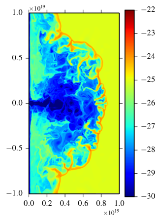
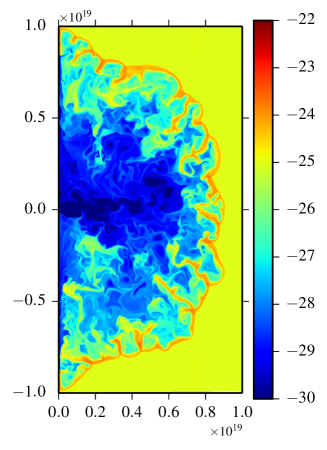
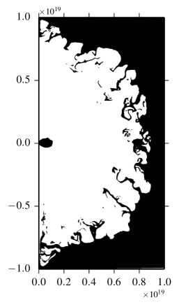
Figure 1: Rayleigh-Taylor “fingers” in 2D simulations. The left and middle panels show $\log_{10}\rho$ at $t\simeq 1060$ years in simulation runs B1 (left) and A1 (middle). Note that in the low magnetization A1 run ($\sigma_{0}=0.01$) the jet is not able to penetrate far into the SNR. The right-hand panel illustrates the way of determining the nebula radius $r_{\rm n}$. It shows the mask used in order to separate PWN from the supernova shell. The nebula radius is then obtained as the volume average $r_{\rm n}=\left(3V/4\pi\right)^{1/3}$. The conspicuous “fingers” form via the Rayleigh-Taylor (RT) instability of the contact discontinuity between the PWN and the supernova shell. The typical “mushroom” morphology of the RT-fingers, characteristic of the non-linear stages of this instability, is not seen here, most likely because of the interaction with the turbulent flow of PWN.

3 Results

One of the important results of Porth, Komissarov & Keppens (2014) is that the global dynamics of axisymmetric 2D models and that of 3D models with strong magnetization of the pulsar wind differ dramatically. The 2D models develop strong axial compression and produce powerful polar outflows. This results in a highly elongated shape of the nebula. This is in sharp contrast with the observations of the Crab Nebula, which is only moderately elongated. In contrast, the total pressure distribution of 3D models is almost uniform and their shape remains approximately spherical. For 2D models to remain approximately spherical, the magnetization of the pulsar wind should be low. From the perspective of studying the RT-instability in 2D, it looks like this makes us choose between two “evils” – either to focus on the high-sigma models with their unrealistic overall geometry or on the low-sigma models with potentially weaker magnetic field in the nebula. Given the results of previous studies, the magnetic field strength can be important for development of the RT-instability (Jun, Norman & Stone, 1995; Stone & Gardiner, 2007; Bucciantini et al., 2004). To clarify this issue we run two models, A1 and B1, which differ only by the wind magnetization (both these models were studied in Porth, Komissarov & Keppens (2014)). It turns out that the RT-instability yields very similar filamentary structure in these two cases everywhere apart from the polar zones, as one can see in figure 1, which illustrates the solutions at the time $t\simeq 1060\,$yr.

There are two main reasons behind this similarity of A1 and B1 models. First, in axial symmetry, the azimuthal magnetic field has no effect on the growth of RT perturbations as there is no mode-induced field line bending since $\mathbf{B}\cdot\mathbf{k}=0$. Second, the expansion rate of the nebula in the equatorial direction has not been altered dramatically in the high-sigma B1 model compared to the A1 one. Indeed, the equatorial radii are more or less the same in both models. Given this result, we decided to focus on the low sigma model in the rest of our study.

Figure 1 shows a number of anticipated features. Similar to what was found in Jun (1998), we see that 1) the initially spherical shock front is now heavily perturbed and bulges out between the RT fingers; 2) some of the filaments become detached from the shell; 3) the filaments do not exhibit the “mushroom caps” characteristic of the single-mode simulations (Jun, Norman & Stone, 1995). However, in contrast to Jun (1998), we do not see significant density enhancements at the heads of the filaments. Moreover, the filaments extend much further into the nebula in our simulations, up to the distance of up to $1/4\,r_{\rm n}$, which is much closer to the value of $1/3\,r_{\rm n}$ deduced for the Crab Nebula. Visually, the scale of the shock ripples is also not that far away from the observed one.

Although these results looked very encouraging, it was not clear what exactly set the scale found in the simulations. In contrast to the previous studies we did not impose any perturbations of the shock front at the beginning of the runs. Instead, the RT mechanism amplified perturbations which had been imparted on the shock by the unsteady flow inside the PWN bubble. Visual inspection of Figure 1 hints that the scale of the dominant RT-modes could be related to the size of the termination shock, which sets the scale of large-scale eddies emitted by the shock into the PWN. On the other hand, numerical viscosity could also set the scale.

As in any numerical study, it is imperative to check the resolution dependence of our results. Increased resolution leads to a reduction of the numerical viscosity which in turn can influence the instability growth. The numerical viscosity of our third order reconstruction scheme is expected to scale linearly with resolution, a behavior established for example in high order WENO-type schemes (Zhang et al., 2003). The scaling of the viscous growth rate in the Rayleigh-Taylor problem is well known (e.g. Kull, 1991, and references therein) and leads to

$$k_{m}\propto\nu^{-2/3}$$ (8)

for the wave-number of the fastest growing mode. In terms of the wavelength and cell size this reads as $\lambda_{\rm m}\propto\Delta x^{2/3}$. It is much more difficult to predict the outcome in the nonlinear regime because of the earlier saturation of small wavelength modes and the possible inverse cascade.

In order to study the role of resolution in the nonlinear regime, we run three more models A0, A2, and A3, which differ from the A1 model only by the numerical resolution inside the PWN bubble (see table 1). Figures 2 and 3 show the density distribution found in these models. One can see that while the size of the termination shock in all of them is more or less the same, with increasing resolution the power of RT features is progressively shifted towards smaller scales - the forward shock becomes more rounded and the RT-fingers become more numerous and small scale.

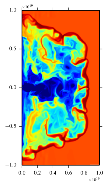
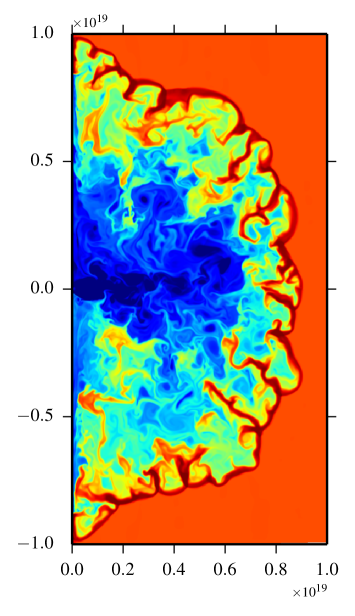
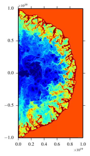
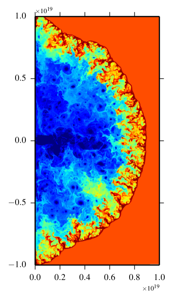
Figure 2: Logarithmic densities showing the entire nebula and filaments at $t\simeq 1060\,\rm years$ with increasing resolution. The models shown here are A0 (top left), A1 (top right), A2 (bottom left) and A3 (bottom right). Each next model has twice the resolution of the previous one.

In order to quantify the dominant scales, we analyze the surface mass density distribution defined via the integral

$$\Sigma(\theta)=\int_{0.6r_{\rm n}}^{1.2r_{\rm n}}\rho(r,\theta)r^{2}dr\,.$$ (9)

Then we subtract the mean value, $\Delta\Sigma(\theta)=\Sigma(\theta)-\bar{\Sigma}$, and use the Fourier decomposition to obtain the power spectrum $P(\Delta\Sigma)(m)$ of the residual fluctuations.

The results are shown in figure 4 together with the low-pass-filtered data. They confirm our naked eye observation of the power transfer to smaller scale features with increasing resolution. In addition, one can see that in all models the spectrum peaks around $m=10-20$. A secondary peak seems to appear at $m\sim 50$ in the model A2 and move to $m\sim 40$ in the model A3.

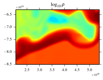
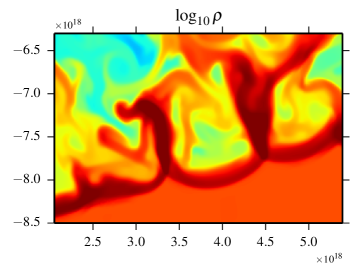
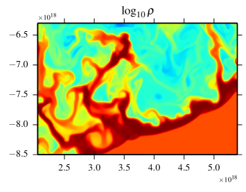
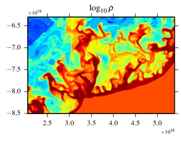
Figure 3: Zoomed in views of logarithmic densities showing the southern shell and filaments with increasing resolution to illustrate the “filament trees”. Simulations A0, A1, A2 and A3 (top to bottom) are shown at $t\simeq 1060~{}\rm years$.

The growing power of small scales with numerical resolution can be interpreted as a result of weaker dampening of small scale RT perturbations by numerical viscosity. On the other hand, visual inspection of plots in figure 2 also shows that at higher resolution the size of eddies reaching the RT interface is also reduced, via development of the turbulent cascade. This could be an additional factor in favor of small scale RT modes, as the initial perturbations imparted on the RT shell at large scales become weaker, and so require more time to reach the non-linear regime. Moreover, smaller scale eddies are also less powerful and smaller scale RT-fingers can survive interactions with them.

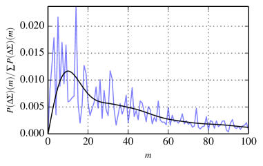
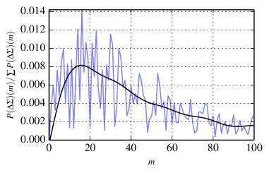
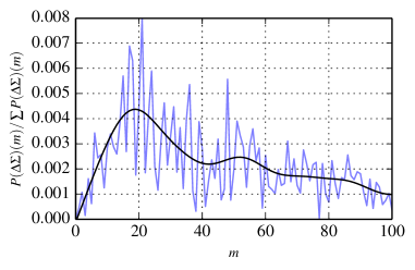
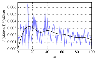
Figure 4: Angular spectra of the surface-density with increasing resolution. The data for models A0, A1, A2 and A3 (left to right, top to bottom) are shown for $t\simeq 1060~{}\rm years$.

Figure 5 illustrates the time evolution of the RT mixing layer in the highest resolution model A3. In order to interpret the data correctly, one has to recall that due to the fixed linear resolution, the angular resolution increases in time following the increase of the linear size of the nebula. This complicates the matter. The time $t=100$ plot shows relatively small scale perturbations in the thin dense layer of shocked ejecta (at $r/r_{n}\sim 1$) reaching the saturation regime. This plot also shows much longer and less dense structures curling around the PWN eddies in the region $0.6\!<\!r/r_{n}\!<\!1$. These features are likely to be the result of entrainment of the shell matter by the fast flow inside the PWN bubble and not RT fingers. Such features have been observed in earlier low-resolution 2D simulations, e.g. the very long “fingers” associated with the backflow of polar jets (see figure 6 in Komissarov & Lyubarsky (2004)). At $t=300$, the RT-fingers proper are becoming more prominent. They are much longer and occupy the region $0.8\!<r\!/r_{n}\!<\!1$. The angular scale of the shock ripples is also noticeably higher.

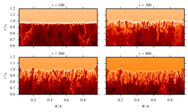
Figure 5: Temporal evolution of the filaments for simulation A3 in the self-similar frame. We show the quantity $\log_{10}r^{2}\rho$ for the simulation times $t\in\{100,300,500,800\}$. The non-linear evolution starting at $t\approx 100$ is governed by the merging of established filaments to form larger scales as well as fragmentation of bubbles and filaments, constantly re-filling fast-growing small scale structure. The thickness of the mixing layer saturates at $\sim 20\%$ of the nebula radius.

At $t=500$ and 800, one can see the fragmentation of large scale shock ripples and large filaments, facilitated by the higher effective Reynolds number of the expanding system. The increase in Reynolds number can also be seen in the progressively smaller eddies in the PWN proper. Fragmentation and inverse cascade of the non-linear RTI compete over the dominant scale of filaments and it is not obvious which process has the upper hand at any given time. This is visualised in figure 6, showing the time-evolution of the scale containing the most mass.

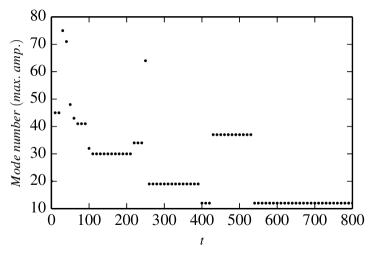
Figure 6: Mode number of the most massive scale as a function of simulation time in run A3.

Initially, the dominant mode number is small-scale, owing to the faster linear growth of small scale structure. The inverse cascade is obtained in the non-linear phase where the larger scales overtake the saturated small scales. However, this trend is reversed at times $t\simeq 200$ and $t\simeq 400$ where we observe a sudden increase in the dominating mode number, owing to the creation of new small scale features.

While the structure of the filaments in $\theta$-direction thus shows some resolution-dependence, the resulting transport of SNR material into the PWN is largely unaffected by resolution effects. Figure 7 shows the radial distribution of SNR material defined via

$$\langle dM/dr\rangle_{\theta}=\frac{1}{\pi}\int_{0}^{\pi}2\pi r^{2}\rho_{\rm SNR}\sin\theta d\theta\,.$$ (10)

At $t\simeq 950\,\rm years$, the mixing region ranges from $6\times 10^{18}\rm cm$ to $\sim 7.5\times 10^{18}\rm cm$ and the radial distribution agrees particularly well in the inner part. Further outside, the distribution becomes increasingly peaked for higher resolution, in agreement with the increasingly circular appearance of the nebula. In front of the PWN-shock, the SNR evolves according to the self-similar expansion law $\rho_{\rm SNR}\propto t^{-3}$ in good agreement with the simulations.

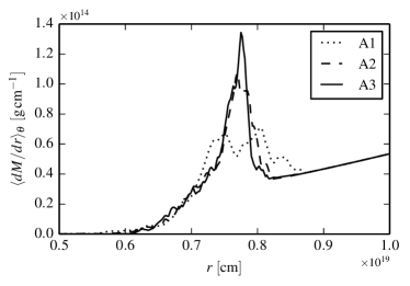
Figure 7: Radial distribution of SNR material at $t\simeq 950\ \rm years$ for simulation runs {A1,A2,A3}.

Visual inspection of the animated data (see the online material) suggests that the inverse cascade is also present in the simulations – occasionally smaller scale ripples merge and create a larger one. When this occurs, one can see several RT fingers emerging from the same base. The plot for the A3 model in figure 3 shows an example of such a structure (its base coordinates are $r=3.4$, $z=-8.0$). Figure 8 provides more information on the stucture of simpler configurations, where only one or two fingers are found at the junction of two shock ripples. Interestingly, the total pressure measured at the base of some fingers is significantly higher than in the surrounding plasma, with a sharp rise, characteristic of a shock wave. In order to check the shock interpretation, we studied the velocity field in the frame moving with the velocity measured at the base of the left finger, indicated in the figure by a cross. This velocity is subtracted from the velocity field measured in the original lab-frame and the result is presented in the figure 8. This allows us to see clearly the flow converging towards the finger base. The Mach number is above unity upstream of the base and drops below unity downstream, inside of the high pressure region. Thus, the results are consistent with the shocked ejecta plasma sliding with slightly supersonic speed along the ripples towards their junction point, where it passes through two stationary shocks before entering the finger. Vortical motion in the space between the neighbouring fingers may also contribute to the finger overpressure.

The plasma-beta at the filament base varies greatly (lower right panel), with minimal values larger than $\simeq 10$ and maximal values – in regions where mixing is advanced – ranging up to $10^{4}$. In simulation B1 with $100\times$ stronger wind magnetisation, with the exception of the spurious jet region where $0.1<\beta<1$, we still observe similar values of the interface plasma beta, due to annihilation of flux loops with opposite polarity in the nebula. Thus we do not expect strong suppression of field-aligned modes, as the critical angular scale becomes $\theta_{c}/\pi\lesssim 1/40$ ( see Eq. 6) in the bulk of the nebula.

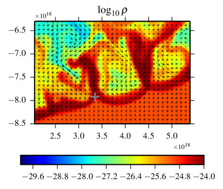
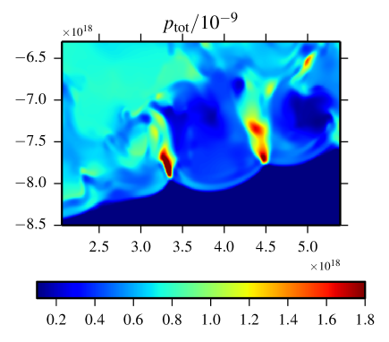
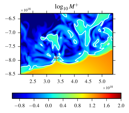
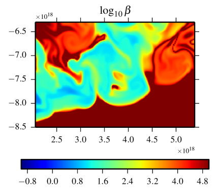
Figure 8: Zoom into the southern filaments of run A1 ($t\simeq 1060\rm~{}years$). The top-left panel shows the logarithmic rest-frame density with flow field vectors and the top-right panel the total pressure. Sonic Mach-number with white contour on $M^{+}=1$ is shown in lower left and the ratio of gas and magnetic pressures, $\beta=P_{g}/P_{m}$, is given in the lower right panel. Note that velocity vectors and Mach number $M^{+}$ are shown relative to the rest-frame of the pivot-point indicated by grey “+”.

4 Discussion

The convergence study of the RT-instability described in the previous section indicates that with higher resolution, the filamentary structure produced in the simulations becomes less similar to the one observed in the Crab Nebula, with the deficit of large-scale structure being the most pronounced discrepancy. In this section, we discuss the possible explanations of this result and speculate on the origin of the Crab’s large-scale filaments.

As we have already commented on in the Introduction, the radial expansion of the RT interface in our problem, introduces a number of interesting modifications to the classical results obtained in plane geometry. Here we derive them via adjusting in a rather crude but very simple way the non-relativistic results in planar symmetry. More accurate analysis of the linear theory can be found elsewhere (Binnie & Taunt, 1953; Gupta & Lawande, 1986; Chevalier & Fransson, 1992; Goedbloed, Keppens & Poedts, 2010). We start with the non-magnetic case and discuss the potential role of magnetic field later.

We denote as $\theta_{m}=\lambda/r_{n}$ the angular scale of RT perturbations. Here $r_{n}\propto t^{\delta}$, where $\delta=6/5$, is the mean radius of the nebula at the phase of self-similar expansion. As the nebula expands radially, $\lambda$ increases proportionally to $r_{n}$, but $\theta_{m}$ remains constant. This linear stretching of the perturbations is most important. First, the linear amplitude of perturbations, $h$, is no longer the most suitable parameter to describe their strength and should be replaced with $x=h/\lambda$. Assuming that $h$ grows at the same rate as in the plane case with $A=1$ we find

$$\dot{x}=x\left[\frac{\dot{h}}{h}-\frac{\dot{r}_{n}}{r_{n}}\right]=\kappa\frac{x}{t}\,,$$ (11)

where

$$\kappa=\omega-\delta=\left(\frac{2\pi\delta(\delta-1)}{\theta_{m}}\right)^{1/2}-\delta\,.$$

This shows that the amplitude growth is a power law, $x\propto t^{\kappa}$, and suggests the critical angular scale

$$\theta_{s}=\frac{2\pi(\delta-1)}{\delta}$$

above which the perturbations do not grow. For $\delta=6/5$, corresponding to a uniform ejecta and constant wind power, $\theta_{s}=\pi/3$. More accurate analysis of RTI in spherical geometry yields the growth rate

$$\omega^{2}=\frac{lg}{r_{n}}\,,$$ (12)

where $l$ is the degree of the associated Legendre polynomial $P^{m}_{l}(\cos\theta)$ (Binnie & Taunt, 1953; Gupta & Lawande, 1986). In the limit of high $l$ we should recover the plane geometry which leads to the identification of the wavenumer $k$ with $l$ via $k=l/r_{n}$. Using this we find the critical degree $l_{s}=6$ which corresponds to $\theta_{s}=\pi/3$. This is very close to the critical degree $l_{s}=5$ found in the thin shell approximation (Chevalier & Fransson, 1992), showing that the dumping of the RT instability at large scales is a robust result. Based on this we tentatively conclude that there is an upper limit of $\simeq 50^{\circ}$ for the angular size of perturbations above which they do not grow.

The solution to Eq. (11), $x(t)=x_{0}(t/t_{0})^{\kappa}$, implies that a perturbation of any amplitude imposed at the time $t_{0}$ will be able to reach the non-linear regime provided $t_{0}$ is sufficiently small. For the Crab Nebula this means that we should be dealing with the fully nonlinear regime on all scales. However, in our simulations where $t/t_{0}$ is not particularly high, some large-scale perturbations may still be growing in the linear regime. For example, according to this result, the largest angular scale to grow by a factor of $e$ during our simulation time is $\pi/4.4$. Moreover, one may reasonably expect their final amplitude to depend on the strength of large-scale motion inside the PWN bubble as it is responsible for the initial amplitude of these perturbations. The reduction of the final amplitude with resolution, observed in our simulations, may well reflect the parallel weakening of this large scale motion.

Since in the real Crab Nebula the perturbations of all scales which are linearly unstable, are expected to have reached the nonlinear regime, this regime is much more relevant for interpretating the observations. To this end, consider the growth of RT bubbles in the non-linear regime. Substituting $g=\ddot{r}_{n}=\delta(\delta-1)(r_{n}/t^{2})$ into equation (3) and integrating, we find that the bubble height is

$$\frac{h}{r_{n}}\simeq\frac{1}{2}\left(\frac{\theta_{m}(\delta-1)}{\delta}\right)^{1/2}\,.$$ (13)

Thus, the relative height of bubbles, $h/r_{n}$, “freezes out” in the non-linear phase. This conclusion fits nicely the picture of self-similar expansion. The critical scale $\theta_{s}$ of linear regime sets the upper limit on $h/r_{n}$. For $\delta=6/5$ this limit is $(h/r_{n})_{\rm max}\simeq 0.2$, which is about the size for the largest bubbles of the Crab Nebula “skin” (Hester, 2008). The fact that in our simulations we do not observe high amplitude bubbles on these scales may indicate they have not had enough time to reach the non-linear regime yet. The inverse cascade may contribute to the production of large-scale bubbles, but it is unlikely to overturn the freezing-out effect.

Since the finite thickness of the RT unstable layer and the forward shock do not feature in the analyses leading to Eq. (13), this result should not be considered as an accurate prediction yet. However, it gives us a basis to speculate about the origin of the largest “filaments” seen in the Crab Nebula. These features can be as long as the nebula radius and they do not appear to be streaming radially towards its center (see figure 1 in Hester (2008) as well as figure 2 in Clark et al. (1983)) as one would expect for the RT-fingers. Instead they seem to outline a network of very large cells filled with synchrotron-emitting plasma. We propose that these cells are actually the largest RT-ripples (bubbles) on the surface of the Crab Nebula and these filaments designate “valleys”, where these ripples come into contact with each other. The plasma of shocked ejecta may slide along the surface of the ripples into these valleys, in very much the same fashion as we have discussed in connection with figure 8. These filaments may form a base from which proper RT-fingers will stream radially towards the center of the nebula. In fact, this is indeed what is seen in the Crab Nebula, most clearly in its NE section, where a number of smaller scale filaments seem to originate from a large one at the angle of almost 90 degrees. Remarkably, the observed cell size is in a very good agreement with the largest angular scale of shock ripples, $\theta_{s}\simeq\pi/3$, which can be amplified by the RT-instability. These large-scale ripples are not seeded internally by the interaction with the large-scale motion inside the PWN bubble, the only source of perturbations in our simulations. Instead, they may originate from inhomogeneities in the supernova ejecta itself, which we did not incorporate in our models. Given the violent nature of supernova explosions it seems only natural to expect strong large-scale fluctuations in the ejecta (e.g. Couch & Ott, 2013). Moreover, Fesen, Martin & Shull (1992) argued that the conspicuous “bays” in the nonthermal optical emission of the Crab Nebula could be indications of a presupernova disk-like ejection. The interaction of a supernova ejecta with such a disk is believed to be behind the emergence of bright rings around SN 1987 A (Larsson et al., 2011).

As we have noted in the Introduction, the magnetic field may have strong impact on the development of the RT-instability. This may seem particularly significant as pulsar winds inject highly magnetized plasma into the PWN bubble. Even for weakly-magnetised winds, the magnetic effects would be important provided PWN were organised in accordance with the Kennel-Coroniti model. In this model, the initially weak magnetic field is amplified towards equipartition between the magnetic and thermal energies near the contact discontinuity with the shocked supernova ejecta. This is exactly the condition for inhibiting the RTI as derived in Bucciantini et al. (2004), when considering modes aligned with the magnetic field. In contrast, in our simulations the magnetic field is always normal to the wave vector of any type of perturbation due to their symmetry, which nullifies the magnetic effect and which can be considered as the main limitation of our study. However, this limitation is probably not as important as it seems. Strong magnetic dissipation seen in our simulations, particularly in the 3D models (Porth, Komissarov & Keppens, 2013, 2014), keeps the magnetic field well below the equipartition near the interface even for high-sigma pulsar winds. Moreover, in 3D the magnetic field is not that effective in inhibiting the RTI, as matter can slide in between the magnetic field lines without bending them downwards (Stone & Gardiner, 2007). The combination of these factors makes us conclude that the impact of magnetic field on the development of RTI in the Crab Nebula is likely to be rather minimal, which is consistent with the observations.

Apart from the high magnetization employed in some runs, the setup of our simulations is very similar to that of the previous axisymmetric simulations of PWN, e.g. by Komissarov & Lyubarsky (2003, 2004); Del Zanna, Amato & Bucciantini (2004); Bogovalov et al. (2005); Camus et al. (2009). However, none of those captured the development of the RT-instability. We believe that this is due to the insufficient resolution of previous studies at the interface between the PWN and the supernova shell. This is not surprising as these studies were mainly concerned with the inner regions around the termination shock and used spherical coordinates which fit the purpose nicely. However, their spatial resolution thus quickly decreases with the distance from the origin. In contrast, in the cylindrical coordinates employed here, we obtain uniform resolution throughout the PWN ($\Delta r=\Delta z=1.95\times 10^{16}\,\rm cm$). Moreover, we utilize third order spatial reconstruction and Runge-Kutta time-stepping giving overall higher accuracy compared to the previous studies.

5 Conclusions

Our high resolution axisymmetric simulations of PWN now reveal intricate structures of filaments growing via the Rayleigh-Taylor instability of the contact discontinuity between PWN and SNR. Given the high rate of magnetic dissipation observed in recent 3D simulations of PWN, the magnetic tension is likely to play only a minor role in the RTI such that our axisymmetric simulations are in fact applicable to reality.

In application to the Crab nebula, we have simulated the last 800 years of its evolution and find the longest fingers to reach a length of $\sim 1/4$ of the nebula radius. The inverse cascade observed in the planar RTI is complemented by constant replenishment of small scale structure due to fragmentation of old filaments and formation of new fast growing small scale perturbations. The latter is particularly pronounced at the large “bubbles” of the nebula which, as they expand along with the nebula provide favourable conditions for growth of fresh small-scale RTI.

The most massive filaments in our simulations reach a scale of $m\simeq 15$ (corresponding to 15 large fingers over the semi-circle), independent of the numerical resolution. Our simulations can not yet reproduce the largest scales observed in the Crab nebula and we propose that they must be seeded from inhomogeneities in the SNR as would result from an anisotropic supernova explosion.

In the future, we plan to investigate the influence of magnetic tension on the filamentary network in local 3D simulations of PWN with realistic values of the magnetisation.

6 Acknowledgments

SSK and OP are supported by STFC under the standard grant ST/I001816/1. SSK has been partially supported by NASA grant NNX13AC59G. SSK acknowledges support by the Russian Ministry of Education and Research under the state contract 14.B37.21.0915 for Federal Target-Oriented Program. RK acknowledges FWO-Vlaanderen, grant G.0238.12, and BOF F+ financing related to EC FP7/2007-2013 grant agreement SWIFF (no.263340) and the Interuniversity Attraction Poles Programme initiated by the Belgian Space Science Policy Office (IAP P7/08 CHARM). The simulations were carried out on the Arc-1 cluster of the University of Leeds.

References

- Bietenholz et al. (1991) Bietenholz M. F., Kronberg P. P., Hogg D. E., Wilson A. S., 1991, ApJ, 373, L59
- Binnie & Taunt (1953) Binnie A. M., Taunt D. R., 1953, Proceedings of the Cambridge Philosophical Society, 49, 151
- Bogovalov (1999) Bogovalov S. V., 1999, A&A, 349, 1017
- Bogovalov et al. (2005) Bogovalov S. V., Chechetkin V. M., Koldoba A. V., Ustyugova G. V., 2005, MNRAS, 358, 705
- Bogovalov & Khangoulian (2002) Bogovalov S. V., Khangoulian D. V., 2002, MNRAS, 336, L53
- Bucciantini et al. (2004) Bucciantini N., Amato E., Bandiera R., Blondin J. M., Del Zanna L., 2004, A&A, 423, 253
- Camus et al. (2009) Camus N. F., Komissarov S. S., Bucciantini N., Hughes P. A., 2009, MNRAS, 400, 1241
- Chandrasekhar (1961) Chandrasekhar S., 1961, Hydrodynamic and hydromagnetic stability