Control and diagnosis of temperature, density, and uniformity in x-ray heated iron/magnesium samples for opacity measurements

Abstract

Experimental tests are in progress to evaluate the accuracy of the modeled iron opacity at solar interior conditions, in particular to better constrain the solar abundance problem [S. Basu and H.M. Antia, Physics Reports 457, 217 (2008)]. Here we describe measurements addressing three of the key requirements for reliable opacity experiments: control of sample conditions, independent sample condition diagnostics, and verification of sample condition uniformity. The opacity samples consist of iron/magnesium layers tamped by plastic. By changing the plastic thicknesses, we have controlled the iron plasma conditions to reach i) $T_{e}$=167$\pm$3 eV and $n_{e}=\mathrm{\left(7.1\pm 1.5\right)\times 10^{21}\,cm^{-3}}$, ii) $T_{e}$=170$\pm$2 eV and $n_{e}=\mathrm{\left(2.0\pm 0.2\right)\times 10^{22}\,cm^{-3}}$, and iii) $T_{e}$=196$\pm$6 eV and $n_{e}=\mathrm{\left(3.8\pm 0.8\right)\times 10^{22}\,cm^{-3}}$, which were measured by magnesium tracer K-shell spectroscopy. The opacity sample non-uniformity was directly measured by a separate experiment where Al is mixed into the side of the sample facing the radiation source and Mg into the other side. The iron condition was confirmed to be uniform within their measurement uncertainties by Al and Mg K-shell spectroscopy. The conditions are suitable for testing opacity calculations needed for modeling the solar interior, other stars, and high energy density plasmas.

I Introduction

Opacity quantifies photon absorption in matter and plays a crucial role in many high energy density (HED) plasmas, including inertial fusion plasmas and stellar interiors. Modeling opacity is especially challenging when the plasma is composed of partially-ionized atoms with many bound electrons. First, one must accurately compute atomic data (e.g., energy level structures, photoionization cross-sections, and oscillator strengths); then, atomic level populations have to be computed for the given conditions including a sufficiently-complete set of atomic levels; and finally, line shapes and spectral formation must be taken into account in order to compute the frequency-dependent opacity. The complexity of such models makes experimental tests critical. However, the range of plasma conditions where opacity models are experimentally validated is extremely limited because opacity measurement requirements are also challenging. Opacity measurements at HED conditions, such as those found in stellar interiors and inertial fusion ablators, are particularly rareBailey et al. (2009).

Without accurate opacity measurements, the systematic uncertainties of modeled opacities are not known. This limits our understanding of plasmas and sometimes complicates the interpretation of plasma hydrostatic/hydrodynamic simulations when they disagree with measurements or observations. Around 1980, it was reported that simulated Cepheid variable stars could not reproduce the observed pulsations in certain regimesCox (1980). In an attempt to resolve the discrepancies, various modifications to the Cepheid models were tested, such as reducing mass, increasing helium abundance, and introducing magnetic fields. However, it turned out that the discrepancies were not caused by the Cepheid models but mostly by inaccuracy of the calculated opacities used in the models. Opacities re-computed using improved models were significantly larger at Cepheid envelope conditions and resolved the discrepanciesIglesias et al. (1987, 1990); Rogers and Iglesias (1993). Calculating opacities is difficult, and this example illustrates the possible consequences of their inaccuracy.

More recently, calculated solar interior opacities, especially at the base of the solar convection zone (CZ), are in questionBailey et al. (2009). Standard solar models (i.e., hydrostatic models) were in excellent agreement with helioseismic measurements until the solar metal abundances were reduced in early 2000s Asplund et al. (2005); Basu and Antia (2008); Asplund et al. (2009); Basu and Antia (2013). This lowered the abundances of C, N, O, Ne, and Ar by 35-45%, which lowered the calculated solar mixture opacities accordingly. The downward shift in the opacity altered the radiative heat transfer in the solar models, affecting their agreement with helioseismic measurements, especially at the CZ base (i.e., $R\sim 0.713R_{SUN}$)Basu and Antia (2008). As with the Cepheid variable problem, the inaccuracy of calculated opacity has been suggested as the origin of this CZ problem; a 10-30% increase in opacity would bring solar models and helioseismology into agreementBasu and Antia (2008).

Until high-accuracy opacity measurements are conducted, opacity uncertainty will continue to be a potential explanation for many HED and astrophysical model-observation discrepancies. While a discrepancy often suggests how much the mean opacity should be increased (or decreased), it does not provide anything conclusive on calculated opacity accuracy. Are the discrepancies really caused by opacity inaccuracy? Exactly how are calculated opacities different from true opacities? Performing benchmark experiments measuring opacity is crucial to answer these questions and to guide potential opacity model refinements. Such refinements would help to improve our understanding of the Sun, many other stars, and a variety of other HED plasmas.

Opacity measurement techniques have been developed and refined over the past two decadesPerry et al. (1996); Davidson et al. (1988); Perry et al. (1991); Foster et al. (1991); Chenais-Popovics et al. (2001); Bailey et al. (2003); Renaudin et al. (2006); Da Silva et al. (1992); Springer et al. (1992); Winhart et al. (1995); Springer et al. (1997); Chenais Popovics et al. (2000). Nevertheless, performing reliable experiments is demanding, and few high quality measurements exist. There are many sources of difficultyPerry et al. (1996); Bailey et al. (2009). First, one has to tailor the sample to the target conditions while also achieving sample uniformity, steady state, and local thermodynamic equilibrium (LTE). When transmission is measured through significant gradients, it is difficult to derive definitive conclusions on opacity. Steady state and LTE are common assumptions in opacity models, and thus have to be realized in the sample. To achieve LTE, the experiment must either reach high densities or include a strong external radiation field that is reasonably close to equilibrium with the sample plasma, and these conditions must be maintained over a duration sufficient to establish steady-state (i.e., $df_{i}/dt\sim 0$ for each level population $f_{i}$). Second, once the sample is tailored to the target conditions, the sample transmission has to be accurately measured. To benchmark the detailed atomic and plasma physics in modern opacity models, it is necessary to measure the frequency-resolved transmission. This requires a backlighter that is bright, to mitigate the sample self-emission effects on the emergent transmission spectraPerry et al. (1996); Bailey et al. (2009), and spectrally smooth, to avoid unnecessary complications due to instrumental broadeningIglesias (2006). Reliable frequency-resolved opacity measurement also requires spectrometers with high resolving power to observe detailed bound-bound line features. These spectrometers must be free of any artifacts such as crystal defects and film scanning flaws that could result in disturbing the data. Finally, the Fe plasma conditions have to be independently measured to model the Fe opacity and compare it with the measurement.

In 2007, Fe opacity experiments were performed to constrain the CZ problem discussed earlier, and Fe transmission spectra were successfully measured at charge state distributions similar to Fe at the CZ base for the first timeBailey et al. (2007). Fe was studied for two reasons. First, Fe is one of the biggest opacity contributors at the CZ base. Second, Fe at the CZ base has many bound electrons, making it more difficult to model than many other elements in the solar matter. Uncertainty of modeled Fe opacity may therefore be larger than the other elements. The Fe samples were heated by the z-pinch dynamic hohlraum (ZPDH) radiation source at the Sandia National Laboratories Z-machine. The backlighter was provided by the stagnation of the ZPDH implosion and was characterized as a smooth 314 eV blackbody radiator. This backlighter was bright enough to mitigate sample self-emission at the measured Fe conditions. The Fe reached an electron temperature, $T_{e}$, of 156 eV and an electron density, $n_{e}$, of 6.9$\times$10${}^{21}\,\mathrm{cm^{-3}}$. The conditions were independently measured by K-shell transmission spectroscopy of Mg mixed with the sample. Fe L-shell transmission spectra computed from detailed opacity models were shown to match reasonably well with the measurements.

In order to benchmark Fe opacity models at the CZ base, more experiments are needed. First, while the Fe transmission spectra were measured at the charge state distribution similar to that of Fe at the CZ base, the inferred $T_{e}$ and $n_{e}$ were significantly lower than the conditions at the CZ base (i.e., 185 eV and 9$\times$10${}^{22}\,\mathrm{cm^{-3}}$). Thus, Fe opacity models need to be tested at higher $T_{e}$ and $n_{e}$ . This is important because additional effects become important as $T_{e}$ and $n_{e}$ increase. In LTE, the same average ionization can be achieved by increasing both $T_{e}$ and $n_{e}$. However, since population within each charge state is distributed following the Boltzmann relation, $p_{excited}/p_{ground}\propto\exp\left(-\Delta E/kT\right)$ where $\Delta E$ is the energy difference between the excited and ground states, ions produced by higher $T_{e}$ and $n_{e}$ would produce more population in the excited states. This makes the accuracy of opacity calculations more sensitive to the accuracy of the atomic data of excited levels and to the treatment of highly-excited levels (doubly, triply, .., multiply excited levels). As density increases, high density effects such as ionization potential depression and Stark line broadening become more important. In particular, Stark line broadening in L-shell line transitions has not been explored as extensively as that of K-shell lines. Furthermore, even detailed modern opacity models employ rather simple approximations similar to the formalism discussed in Griem et al.Griem (1968). In order to disentangle these physical details and benchmark opacity models, it is crucial to control the plasma conditions and repeat Fe opacity experiments at several different $T_{e}$ and $n_{e}$ while maintaining similar charge state distributions. Such a collection of measurements would promote investigations of how the effects of higher $T_{e}$ and $n_{e}$ gradually change the opacity and how well opacity models can predict them. It is also important to make direct measurements of the sample uniformity. In Bailey et al.Bailey et al. (2007), the sample uniformity assertion was supported by the use of volumetric heating provided by ZPDH radiation and by the fact that the mixed Fe/Mg transmission spectra were successfully modeled by a single $T_{e}$ and $n_{e}$. However, it is preferable to experimentally quantify the level of the sample non-uniformity.

In this article, we describe measurements addressing three of the key requirements for opacity experiments: i) control of the Fe conditions, ii) independent plasma diagnostics, and iii) verification of the sample condition uniformity. The Fe sample conditions can be controlled by the thickness of the tamping plastic ($\mathrm{CH}$) as suggested by hydrodynamic simulations Nash et al. (2010). Thus, we performed Fe opacity experiments with three different $\mathrm{CH}$ tamper thicknesses: i) 10 $\mu$m, ii) 35 $\mu$m, and iii) 68 $\mu$m. The Fe conditions are independently measured by Mg K-shell spectroscopy and found to be i) $T_{e}$=167$\pm 3$ eV and $n_{e}=\mathrm{\left(7.1\pm 1.5\right)\times 10^{21}\,cm^{-3}}$, ii) $T_{e}$=170$\pm 2$ eV and $n_{e}=\mathrm{\left(2.0\pm 0.2\right)\times 10^{22}\,cm^{-3}}$, and iii) $T_{e}$=196$\pm 6$ eV and $n_{e}=\mathrm{\left(3.8\pm 0.8\right)\times 10^{22}\,cm^{-3}}$, respectively. These conditions nearly reproduced the charge state distribution of Fe at the CZ base, but with different levels of high temperature and density effects. Also, one experiment was designed and performed to directly investigate the sample non-uniformity. For this particular experiment, Al was mixed into the side of the Fe sample facing the radiation source and Mg in the opposite side. Fe conditions in both sides are inferred by Al and Mg K-shell spectroscopy. We confirmed that there is no measurable axial non-uniformity in the Fe sample. The discussion of other requirements, such as steady-state and LTE, as well as details of the transmission determination, the comparison with Fe opacity models, and the implications to astrophysics, atomic physics, and HED physics are beyond the scope of this article and will be discussed elsewhere. Section II discusses the experiments and data reduction. Section III explains the Mg K-shell spectroscopy, how to model the spectra, and how to find the optimal $T_{e}$ and $n_{e}$ from the measured Mg spectra. Section IV summarizes Fe conditions analyzed for experiments using different $\mathrm{CH}$ tamper thicknesses. Section V summarizes the sample non-uniformity investigation.

II Experiments and data reduction

Fe opacity experiments were performed at the Sandia National Laboratories Z-machine. The Fe sample is volumetrically heated by a z-pinch dynamic hohlraum (ZPDH) and backlit at its stagnation. A detailed description of the z-pinch dynamic hohlraum is discussed elsewhereBailey et al. (2006); Rochau et al. . Figure 1(a) illustrates a cross-sectional schematic of the cylindrical ZPDH initial setup. An azimuthal magnetic field is generated by the electrical current, $J$, running through tungsten wires strung in a cylindrical array. The current and self-generated magnetic field produce a $\boldsymbol{J}\times\boldsymbol{B}$ force that pushes the tungsten plasma towards the axis where a 14.5 $\mathrm{mg/cm^{3}}$ cylindrical plastic ($\mathrm{CH_{2}}$) foam is located. When the tungsten plasma collides with the foam, it generates a radiative shock in the $\mathrm{CH_{2}}$ [Fig. 1(b)]. The shock radiation is trapped inside the thick tungsten plasma wall due to the high opacity of the tungsten plasma. The Fe/Mg sample placed on the top exit hole is heated by the hohlraum radiation, and it is backlit when the radiating shock stagnates at the z-pinch axis [Fig. 1(c)].

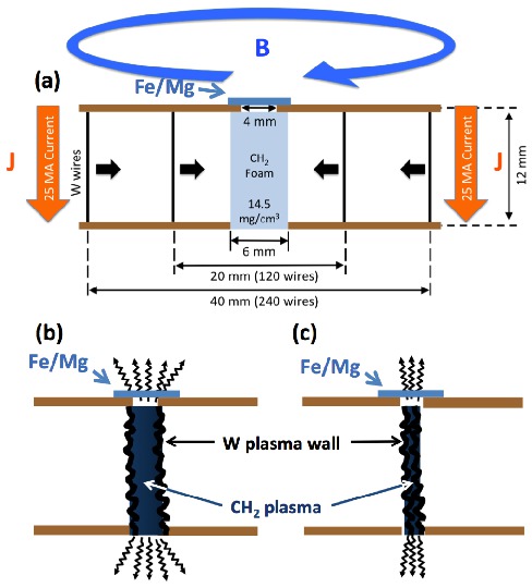
Figure 1: Cross-sectional schematics of the cylindrical z-pinch dynamic hohlraum (ZPDH). (a) Initial setup of the ZPDH, which consists of 360 tungsten (W) wires concentrically arranged at two radii with a cylindrical low-density plastic ($\mathrm{CH_{2}}$) foam located at the z-pinch center. (b) When the imploding W plasma collides with the $\mathrm{CH_{2}}$ foam, shock-generated radiation is trapped inside the high-opacity W plasma wall and heats the sample. (c) At stagnation, it provides an intense backlighter along the cylindrical axis.

Figure 2 illustrates the difference in the ZPDH radiation seen by the sample and our spectrometers. While any point in the Fe/Mg sample sees the entire ZPDH emitting surface, the detector located $\sim$4100 mm away from the radiation source only sees the central region of its surface because the detector view is limited by an aperture and $\sim$50 $\mu$m slits, which are located $\sim$17 mm and $\sim$2000 mm away from the source, respectively. During a ZPDH implosion, the radiation intensity increases while the area of the bright region decreases. The radiation power from the ZPDH exit hole is proportional to intensity times emitting surface area ($P=\int_{A}I\cdot dA$) and thus changes slowly compared to the change in the implosion itself. The heating radiation is energetic: its energy distribution maximum exceeds 700 eV. The Fe sample is almost transparent to this radiation, and is therefore volumetrically heatedBailey et al. (2009). As the implosion continues, the heating radiation power begins to drop as the decrease in emitting area exceeds the increase in intensity. A few nanoseconds after the heating radiation peak, the radiative shock reaches the z-pinch axis, generating extremely bright radiation that provides the backlighter for the transmission measurements [Fig. 2(b)]. While the data are recorded by a time-integrated spectrometer, time resolution is provided by the few-nanosecond duration of the backlighter.

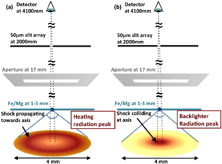
Figure 2: Schematics showing the ZPDH radiation emitting surfaces and the view factors from the samples and the detectors at (a) the time of the heating radiation peak and (b) the time of the backlighter radiation peak. Since each point on the sample sees the entire emitting surface area, the sample experiences maximum radiation (i.e., $\int I\cdot dA$) before stagnation. The detector records most of the radiation during stagnation because its view is limited to the central region by an aperture and 50 $\mu$m slits. The distances specified for the various components are measured from the x-ray source.

The ZPDH backlighter is attenuated by the Fe/Mg sample, and the spectrum is recorded with time-integrated potassium acid phthalate convex curved crystal spectrometers equipped with Kodak RAR2492 x-ray film. The spectrometers have between four and six slits $\sim$2000 mm away from the sample and the backlighter, making the magnification $\sim$1. The typical slit width is $\sim$50 $\mu$m, which provides a spatial resolution of $\sim$100 $\mu$m. The crystal curvature radius is 4 or 6 inches, and an x-ray film is located at 8 cm from the crystal. The spectral dispersion axis is determined by ray tracing using prominent lines as wavelength references. Film optical densities are converted to exposure based on Henke et al. Henke et al. (1984a, b). Filter transmissions and crystal reflectivity are corrected based on the data available from the Center for X-Ray Optics with the instrument geometry effects taken into account.

Recording multiple slit images has several advantages. First, one can increase the signal-to-noise ratio of the data without giving up the instrumental spatial resolution. Second, a single image could be flawed by systematic issues such as crystal defects, slit width variations along its length, or reflectivity variations over the crystal surface. However, these systematic issues are random across the different slit images and can be mitigated by averaging over multiple slit images. For example, Fig. 3 (a) and (b) show two of the six individual slit images of Fe/Mg absorption measurements from a single experiment (z2364) and contain crystal defects at random locations. When averaged over the six slit images [Fig. 3 (c)], those artifacts have been greatly reduced.

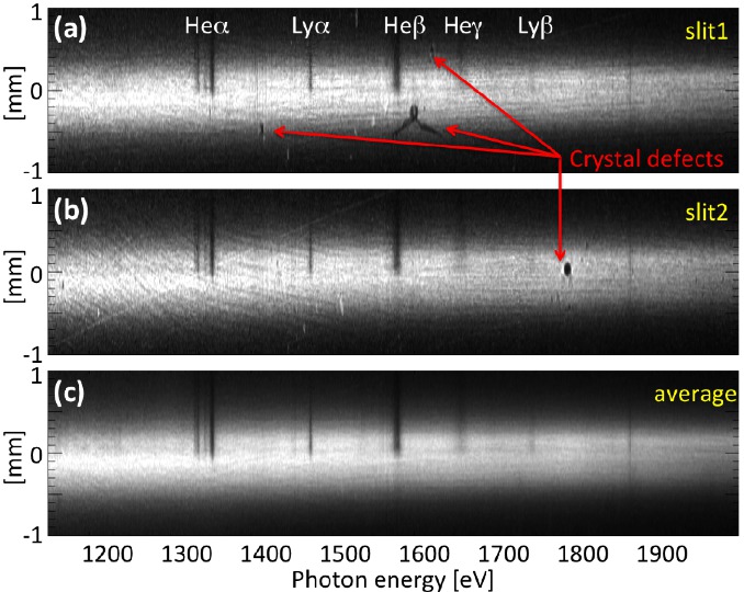
Figure 3: Fe/Mg absorption images over the Mg K-shell spectral range. Strong line features are from Mg K-shell bound-bound line absorptions such as Mg He-$\alpha$, Ly-$\alpha$, He-$\beta$, He-$\gamma$, and Ly-$\beta$. (a) and (b) show two single slit images from z2364, which contain many crystal defects. (c) shows the image averaged over six slit images of the same experiment. Averaging improves the signal-to-noise ratio and helps to mitigate any bias towards individual slit images due to crystal defects or other instrumental problems. The spatial range of interest is from 100 $\mu m$ to 400 $\mu m$ where the backlighter is bright and the Fe/Mg exists in the sample. In this experiment, there is no Fe/Mg in the bottom half of the sample so that we have the option to extract transmission in a single experiment by using the Fe/Mg attenuated spectrum from the top of the image and the unattenuated spectrum from the bottomBailey et al. (2009).

The averaged spectra can be extracted either from the averaged slit image or by averaging the spectra extracted from individual slit images. These two methods are identical as long as the crystal defects are treated in the same way. The uncertainties in the spectra are estimated by taking the standard deviation of the spectra extracted from N individual slit images divided by $\sqrt{\mathrm{N}}$. An example is shown in Fig. 4. The black and the red curves are, respectively, the averaged spectrum and its uncertainty, which for this data set is approximately $\pm 2.5\%$.

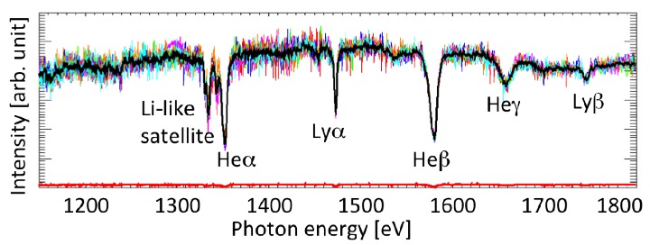
Figure 4: Fe/Mg absorption spectra from a 300 $\mu m$ wide region in Fig. 3. Prominent line features are Mg bound-bound line absorptions such as Mg He-$\alpha$, Ly-$\alpha$, He-$\beta$, He-$\gamma$, and Ly-$\beta$. Six spectra in different colors are extracted from individual slit images. The averaged spectrum is overlaid in black, and its uncertainty is shown at the bottom in red. The average percent uncertainty is $\pm$2.5%.

III Plasma condition determination

Fe conditions have to be measured independently in order to compare the measured Fe transmission with the modeled transmission. Fe conditions predicted by hydrodynamic simulations are not appropriate for this purpose for two reasons. First, we are investigating Fe opacity because the opacity model accuracy has been called into question. Since the sample is heated by radiation in our experiments, the Fe opacity plays a key role in the plasma evolution. If the Fe opacity is in question, we should not expect the hyrdosimulation to predict plasma conditions accurately. Second, hydrodynamic simulations require many input parameters. Providing all of the required information for every experiment is itself a challenge. Propagating all of the input uncertainties to the Fe conditions uncertainties is even more challenging. Thus, we measure Fe conditions directly through K-shell spectroscopy of Mg mixed into the Fe sample.

While L-shell opacity and spectra are not completely understood, particularly at high temperatures and densities, K-shell spectra from H-, He-, and Li-like ions have been extensively researched and used to diagnose plasma conditionsGriem (1992); Hammel et al. (1993); Bailey et al. (2004, 2008). Due to the small number of bound electrons, the required atomic data for singly and multiply excited states can be calculated with high accuracy and fine structure detail. Additionally, many of the atomic data have been experimentally validatedKramida et al. (2013). K-shell line shapes for H-, He-, and Li-like ions have also been extensively investigated over the last 50 yearsBaranger (1958); Smith (1966); Griem (1974); Tighe and Hooper (1978); Mancini et al. (1991); Alexiou (2009); Iglesias and Sonnad (2010); Stambulchik and Maron (2010) and are understood much better than L-shell line shapes. Different K-shell spectral models would infer slightly different $T_{e}$ and $n_{e}$ due to differences in details such as Stark line shape calculation, continuum lowering, atomic data, and numerical approach. The Fe condition uncertainties due to the spectral model details are under investigation and will be discussed elsewhere.

III.1 Temperature and density sensitivity

Line emission from K-shell ions is sensitive to temperature and density. The bound-bound (bb) line transmission is defined as follows:

$$T_{\nu}^{bb}=\exp\left\{-\tau_{\nu}^{bb}\right\}$$ (1)

$$\tau_{\nu,\,lu}^{bb}=N_{Mg}\Delta x\cdot\frac{\pi e^{2}}{m_{e}c}f_{lu}\phi_{\nu,\,lu}p_{l}$$ (2)

where $\tau_{\nu,\,lu}^{bb}$ is the line optical depth at frequency $\nu$ due to photoexcitation from a lower level $l$ to an upper level $u$, $N_{Mg}\Delta x$ is the Mg areal number density measured by Rutherford backscattering, $f_{lu}$ is the oscillator strength of the transition, $\phi_{\nu,\,lu}$ is the line shape associated with the transition, and $p_{l}$ is the fractional population in the lower state of the transition. When the oscillator strengths do not depend on plasma conditions, the only unknowns are $\phi_{\nu,\,lu}$ and $p_{l}$. The line shape, $\phi_{\nu,\,lu}$, is determined by Doppler broadening, natural broadening, and Stark broadening. We also estimated the possible Zeeman effect on the line shape based on an upper limit magnetic field in our experiments. The effect was confirmed to be much smaller than the instrumental spectral resolution and thus neglected in our line shape calculations. At the density of interest here, the dominant line broadening mechanism is Stark broadening, which is sensitive to electron density. Figure 5 shows area normalized line shapes for Mg He-$\gamma$ ($1s^{2}\rightarrow 1s4p$) and Mg Ly-$\beta$ ($1s\rightarrow 3p$) calculated at three different conditions using a detailed Stark line shape calculation code, MERLMancini et al. (1991). One can clearly see that, as electron density increases, the line shapes become broader. This is more significant for the transitions involving high principal quantum numbers, and thus, in this article, the transitions with upper quantum number greater than 2 (e.g., $\beta$, $\gamma$, $\delta$) are used to extract $n_{e}$.

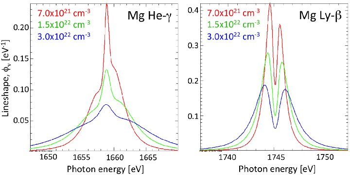
Figure 5: Area-normalized detailed Stark line shapes calculated at $n_{e}$=$\mathrm{7.0\times 10^{21}}$, $\mathrm{1.5\times 10^{22}}$, $\mathrm{3.0\times 10^{22}\,cm^{-3}}$ for (a) Mg He-$\gamma$ and (b) Mg Ly-$\beta$. As density increases, the line shapes become broader.

To diagnose temperature, we use line ratios that reflect the $T_{e}$-dependent ionization balance. The ratio of optical depths integrated over line shapes with $\int\phi_{\nu}d\nu=1$ is:

$$\frac{\tau_{Ly-\beta}^{bb}}{\tau_{He-\gamma}^{bb}} \approx \frac{f_{Ly-\beta}}{f_{He-\gamma}}\frac{p_{1s}}{p_{1s^{2}}}$$ (3)

$$\propto \frac{p_{1s}}{p_{1s^{2}}}$$

where $f_{Ly-\beta}$ and $f_{He-\gamma}$ are the oscillator strengths of Ly-$\beta$ and He-$\gamma$ line transitions, respectively. Since the H-like ground state population and He-like ground state population are directly affected by charge state distributions, their ratio is a strong temperature diagnostic at a given density. Figure 6 shows Mg He-$\gamma$ and Ly-$\beta$ line transmissions computed at $T_{e}$=160, 165, and 170 eV with a fixed electron density $n_{e}$=$\mathrm{8.0\times 10^{21}\,cm^{-3}}$ using a collisional radiative model, PrismSPECT in LTE modeMacFarlane and al (2003); MacFarlane et al. (2007). As the temperature increases from 160 to 170 eV, the He-like ground state population, $p_{1s^{2}}$, decreases by 4% (0.831$\rightarrow$0.794) while the H-like ground state population, $p_{1s}$, increases by about a factor of two (0.051$\rightarrow$0.100), monotonically increasing the ratio of these initial states, $p_{1s}/p_{1s^{2}}$, from $6.1\times 10^{-2}$ to $\mathrm{12.6\times 10^{-2}}$. Thus, from Eq. (3), one can see that relative line strengths from adjacent charge states are strongly dependent on the electron temperature.

Due to the monotonic relationships between line shapes and $n_{e}$ and between line ratios and $T_{e}$, the measured Mg lines constrain the $T_{e}$ and $n_{e}$ of the Mg embedded region. Since Mg is mixed throughout the Fe sample, the Fe plasma conditions can be inferred from the Mg K-shell lines.

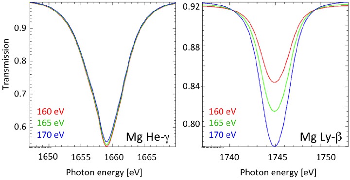
Figure 6: Mg He-$\gamma$ and Ly-$\beta$ transmissions at $T_{e}$=160, 165, and 170 eV with a fixed electron density $n_{e}$=$8.0\times 10^{21}\mathrm{\,cm^{-3}}$. As temperature increases, the line ratio changes due to the change in ionization balance.

III.2 Spectral model and parameter optimization

In the present analysis, Mg spectra are computed by RADIATOR, which is a framework to couple a tabulated emissivity and opacity database with a radiation transport solver and compute emergent spectra by taking into account a given instrumental broadeningNagayama et al. (2012a). This framework is combined with a multi-objective global optimization program, GALMNagayama et al. (2012a), which is based on a genetic algorithm (GA) followed by Levenberg-Marquardt non-linear least squares minimization (LM)Goldberg (1989); Press et al. (1992). The combination of the GA and LM is an efficient optimization algorithm that finds the solution quickly by exploring small fractions of the parameter space.

To use RADIATOR+GALM, two things have to be done: i) create a tabulated emissivity and opacity for Mg and ii) add a radiation transport solver for slab geometry to RADIATOR. The local emissivity and opacity database for Mg is computed by PrismSPECT in LTE mode together with the detailed Stark line shape database computed by MERLMancini et al. (1991). The details on how to extract local emissivity and opacity out of the PrismSPECT calculation are discussed in Appendix A. A general transport radiation solver is developed for slab geometry that can take into account mixtures, linear gradients, background, and self-emission options as needed. While the simple pure transmission approximation is sufficient to extract the sample conditions, the general formalism is useful to investigate various effects on the emergent spectra for many applications and thus is discussed in detail in Appendix B. The formalism is not exclusive to PrismSPECT and can be used with other collisional radiative modelsHansen et al. (2007); Florido et al. (2009). The pure transmission approximation assumes that the backlighter is much brighter than the plasma self-emission and is a slowly changing function of frequency over the instrumental broadening width (Appendix B):

$$T_{\nu}^{\star}=\int g\left(\nu-\nu^{\prime}\right)T_{\nu^{\prime}}d\nu^{\prime}$$ (4)

$$T_{\nu}=\exp\left\{-N_{Mg}\Delta x\cdot\kappa_{\nu}^{PSDB,\,Mg}(T_{e},\,n_{e})\right\}$$ (5)

where the first equation convolves the computed transmission with the instrumental broadening, $g\left(\nu-\nu^{\prime}\right)$, and the second equation is a transmission calculation using a tabulated Mg opacity database computed by PrismSPECT (PSDB). $N_{Mg}\Delta x$ is the Mg areal number density in $\mathrm{ions/cm^{-2}}$, and $\kappa_{\nu}^{PSDB,\,Mg}(T_{e},\,n_{e})$ is the tabulated frequency-dependent Mg fractional absorption coefficient in $\mathrm{cm^{2}/ions}$. $\kappa_{\nu}^{PSDB,\,Mg}$ contains bound-bound (bb), bound-free (bf), and free-free (ff) contributions:

$$\kappa_{\nu}^{PSDB,\,Mg}=\left(\kappa_{\nu}^{bb}+\kappa_{\nu}^{bf}+\kappa_{\nu}^{ff}\right)^{PSDB}$$ (6)

which includes,

$$\kappa_{\nu}^{bb}=\sum_{lu=all\,transitions}\left\{\frac{\pi e^{2}}{mc}f_{lu}\phi_{\nu,\,lu}^{MERL}p_{l}\right\}$$ (7)

The MERL database used in PrismSPECT contains detailed line shapes for Mg He-$\alpha$, $\beta$, $\gamma$, $\delta$, and $\epsilon$, and Mg Ly-$\alpha$ and $\beta$. The ion microfields are computed by APEXIglesias et al. (1985) assuming an Fe:Mg mixture of 1:1. In the temperature range of interest for this work, ion dynamic effects are assumed to be negligible and omitted from the calculation. Both temperature and density sensitivities are encoded in $\kappa_{\nu}^{PSDB,\,Mg}$ via the detailed line shape, $\phi_{\nu,\,lu}^{MERL}$, and the lower population, $p_{l}$, in the $\kappa_{\nu}^{bb}$ contribution. The areal number density $N_{Mg}\Delta x$ controls the line depths. RADIATOR+GALM optimizes $T_{e}$, $n_{e}$, and $N_{Mg}\Delta x$ that best reproduce the measured Mg spectra.

III.3 Instrumental broadening effect on plasma condition diagnostics

While the condition sensitivities exist in $p_{l}$ and $\phi_{\nu}$ of the optical depths $\tau_{\nu}$, what we measure is transmission $T_{\nu}$ convolved with instrumental broadening. One can extract $\tau_{\nu}$ out of $T_{\nu}$ perfectly if and only if the instrumental spectral resolving power is infinite, which is never the case for experiments. The spectral resolving power of our instrument was measured to be $E/\Delta E$$\sim 1000$Loisel et al. (2012). This finite spectral resolution obscures $T_{e}$ and $n_{e}$ sensitivities embedded in the transmissionChenais-Popovics et al. (1990), and lines with higher optical depths lose the sensitivities more significantly by this effect due to the non-linear relationship between $\tau_{\nu}$ and $T_{\nu}$ [Eq. (1)]. The rest of this section synthetically illustrates how our instrumental spectral resolution affects the measured lines, and determines what Mg lines are best used for the Fe plasma $T_{e}$ and $n_{e}$ analysis.

The blue curves in Fig. 7 (a) and (b) are the calculated optical depths, $\tau_{\nu}$, and transmissions, $T_{\nu}$, respectively, for Mg He-$\alpha$ ($1s^{2}-1s2p$), He-$\beta$ ($1s^{2}-1s3p$), and He-$\gamma$ ($1s^{2}-1s4p$) at $T_{e}$=163 eV, $n_{e}$=$\mathrm{8\times 10^{21}\,cm^{-3}}$, and $\mathrm{N_{Mg}\Delta x}\approx 7.4\times 10^{17}\,\mathrm{ion/cm^{2}}$. These are typical conditions achieved in our experiments. While these lines share the same initial state population $p_{1s^{2}}$ in Eq. (2), their optical depths are very different due to the differences in their oscillator strengths and line shapes. When the modeled transmissions are convolved with the instrumental spectral shape, transmissions at the line centers are overestimated, and all the detailed structures are smoothed out as shown in the red curves in Fig. 7(b). One then cannot successfully recover the calculated optical depths when converting from these convolved transmissions, reducing our ability to accurately diagnose $T_{e}$ and $n_{e}$. Red lines in Fig. 7(a) show optical depths converted from transmission with the instrumental spectral resolution effect. One can clearly see that the saturation due to the instrumental broadening affects the stronger lines more. While the He-$\gamma$ line preserves both the shape and the strength, the He-$\alpha$ and $\beta$ lines are heavily altered. The saturation in the He-$\alpha$ is particularly severe and the red line is barely visible in Fig. 7(a). When optical depths are larger than 1, the apparent line shape and strength are strongly affected by instrumental broadening. Thus, in this article, we decided to analyze weaker Mg lines ($\tau_{\nu}\lesssim$1) for the purpose of the iron plasma $T_{e}$ and $n_{e}$ diagnostics.

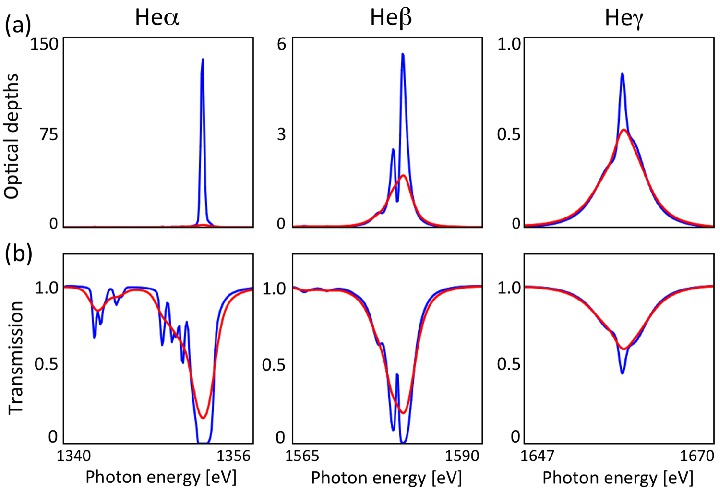
Figure 7: (a) optical depths, $\tau_{\nu}$ and (b) transmission, $T_{\nu}$, of He-$\alpha$, $\beta$, $\gamma$ calculated at $T_{e}$=163 eV and $n_{e}$=$\mathrm{8\times 10^{21}\,cm^{-3}}$ with $N_{Mg}\Delta x\approx 7.4\times 10^{17}\,ions/cm^{2}$. Blue and red curves are before and after the instrumental broadening effects, respectively.

III.4 Mg bound-bound line transmission

Transmission spectra can be extracted by dividing Fe/Mg absorption spectra by unattenuated backlighter spectra. However, fitting the modeled Mg transmission spectra directly to the measured transmission spectra is difficult because the measured transmission has additional Fe attenuation in the Mg b-b line spectral region. Figure 8(a) shows Fe/Mg mixture (red) and pure Mg (blue) synthetic transmission spectra computed at the same conditions. Because of the Fe attenuation, Fe/Mg mixture transmission is lower than pure Mg transmission. Also, while Fe attenuation in this spectral range is smooth and slowly varying with photon energy, there are smooth b-f contributions from Mg above 1700 eV. It is difficult to objectively separate Mg b-f from the Fe b-f in the measured data. Fitting the modeled Fe/Mg transmission spectra to the measured transmission spectra is not ideal because we do not want to rely on calculated Fe opacity to diagnose the Fe conditions. Since plasma condition sensitivity mostly comes from Mg b-b lines as in Eq. 1, one strategy is to extract Mg b-b line transmission spectra both from the measured Fe/Mg spectra and the modeled Mg transmission spectra, and then compare them.

To this end, we first remove Mg b-b lines and then replace them with straight lines to define baselines. By dividing the spectra by the baselines, one can extract Mg b-b line transmission spectra. This removes not only Fe b-f but also Mg b-f from the spectra. For the modeled Mg spectra, we could compute the b-b line transmission for specific lines of interest as in Eq. 1. However, the details of composite spectral formation such as overlapping lines, satellite line contributions, and continuum lowering could affect the instrumental broadening, the baseline determination, and the emergent spectral line shapes. Thus, complete transmission spectra are computed first, and then the baselines are defined to extract b-b line transmission spectra in the same way as for the data. Figures 8(b) and (c) illustrate how baselines are defined for the synthetic data in Fig. 8(a) and how the resultant Mg b-b line transmission spectra agree between Fe/Mg and Mg spectra. The red and blue dashed lines in Fig. 8(b) are the baselines defined for Fe/Mg and pure Mg spectra, respectively. By dividing the spectra by the baselines, Mg b-b line transmission spectra are extracted [Fig. 8(c)]. This study shows that Mg b-b spectra extracted from Fe/Mg spectra are identical to those from pure Mg spectra. Thus, Fe conditions can be inferred by fitting modeled spectra to the measured spectra in Mg b-b line transmissions.

There are two comments on Mg b-b line transmission analysis. One is on the Fe/Mg mixture effects on the emergent spectra. In this article, we assume LTE. In LTE plasmas, level populations are fully determined by $T_{e}$ and $n_{e}$ regardless of whether the plasma is a mixture or not, and mixture effects will only appear in the line shapes via ion microfields contributed from both Fe and Mg ions. As long as mixture effects are included in the Mg Stark line shapes calculation, Mg b-b lines extracted from Fe/Mg spectra and from pure Mg spectra should be identical [Fig. 8(c)]. Another comment is on condition uncertainty due to the baseline determination from the measured spectra. This is a concern because there is noise in the measured spectra. However, baselines are determined based on many data points on both sides of b-b lines, and thus the baseline uncertainty is smaller than the uncertainty of any of those data points. The uncertainty due to the baseline determination is included in the uncertainty due to experiment-to-experiment variation in the following sections.

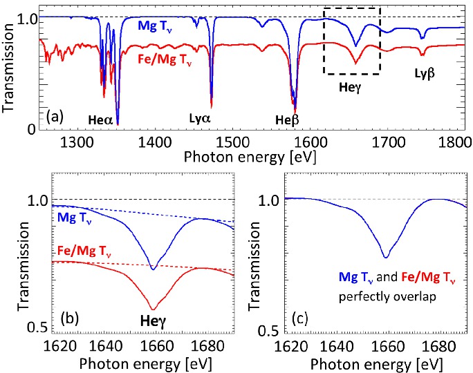
Figure 8: This figure compares calculated transmission spectra from an Fe/Mg mixture (red) and from pure Mg (blue). (a) Fe/Mg transmission is lower than Mg transmission due to additional attenuation by Fe b-f but does not have much Fe b-b contribution except $h\nu<$1450 eV. (b) blow-up of the dashed region of (a). The red and blue dashed lines are baselines defined by replacing the apparent Mg b-b lines by straight lines. (c) Mg b-b line transmission spectra defined by dividing transmission spectra [solid curves in (b)] by the baselines [dashed lines in (b)].

IV Measured Fe plasma conditions

In order to disentangle the complex physical processes included in opacity models and benchmark those models, it is important to measure Fe opacity at different conditions, but with similar charge state distributions. Nash et al. used LASNEX 2DZimmerman et al. (1978) hydrodynamic simulations to explore a way to control Fe sample conditions by changing the target configurationNash et al. (2010). They predicted that the Fe sample $n_{e}$ could be controlled by changing the rear $\mathrm{CH}$ tamper thickness. Adding more tamping mass on the back slows the expansion speed and maintains higher density at the time of the backlight. The slower expansion would also produce modestly higher temperatures.

Based on their suggestions, Fe opacity experiments were performed with three different rear $\mathrm{CH}$ tamper thicknesses as shown in Fig. 9: (a) two experiments with 10 $\mu$m, (b) one experiment with 35 $\mu$m, and (c) six experiments with 68 $\mu$m. By increasing this rear $\mathrm{CH}$ tamper thickness, the backlighter radiation is attenuated more. In order to minimize this extra attenuation, we reduced the front $\mathrm{CH}$ thickness from 10 $\mu$m to 2 $\mu$m for (b) and (c) assuming that Fe/Mg samples do not expand downward due to the pressure provided by the ZPDH $\mathrm{CH_{2}}$ foam plasma.

In this section, we summarize the Fe sample conditions for each target configuration, which are analyzed by Mg K-shell line transmission spectroscopy. Figure 10 (a), (b), and (c) show the Fe/Mg absorption spectra recorded from the different target configurations shown in Fig. 9 (a), (b), and (c), respectively. One can qualitatively observe that Mg K-shell lines become broader as the rear $\mathrm{CH}$ tamper thickness increases, which indicates that $n_{e}$ becomes higher with increasing tamper thickness. For example, He-$\delta$ becomes broader from Fig. 10(a) to (b), and becomes even broader and almost merged into the continuum in (c). Also, He-like satellite lines of Ly-$\alpha$ are not visible in (a), become visible in (b), and even more prominent in (c). These transitions are $1s2p\rightarrow 2p^{2}$ or $1s2s\rightarrow 2s2p$ and start from excited levels. This is proof that, as going from (a) to (c), there is a larger fraction of the population in excited levels and a sign that both $T_{e}$ and $n_{e}$ are higher. This means that the plasma must be hot and dense enough for the collisional excitation rates to be comparable to the spontaneous radiative decay rates. The actual condition of each sample is quantitatively analyzed based on the method discussed in Sec. III.

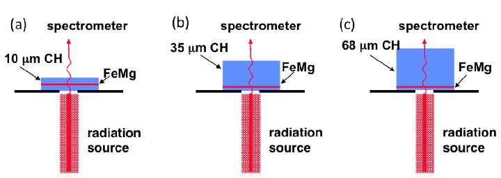
Figure 9: Fe/Mg samples are tamped by three different thicknesses of plastic ($\mathrm{CH}$). (a) rear: 10 $\mu$m, front: 10 $\mu$m (b) rear: 35 $\mu$m, front: 2 $\mu$m, (c) rear: 68 $\mu$m, front: 2 $\mu$m. Based on the hydrosimulation, thicker rear $\mathrm{CH}$ tamper would reach higher $T_{e}$ and $n_{e}$ in Fe/Mg plasmas. The pictures are not to scale, but exaggerated to illustrate the different tamper thicknesses.

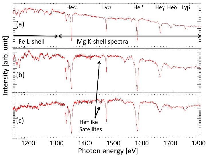
Figure 10: Fe/Mg spectra recorded through the samples with rear $\mathrm{CH}$ tamper thicknesses of (a) 10 $\mu$m, (b) 35 $\mu$m, (c) 68 $\mu$m.

IV.1 10 $\mu$m rear $\mathrm{CH}$ tamper

First, we analyzed Fe conditions using the thin $\mathrm{CH}$ tamper target [Fig. 9 (a)], where the Fe/Mg sample is sandwiched by 10 $\mathrm{\mu m}$ thick plastic. Figure 10 (a) shows the Fe/Mg absorption spectrum from z2301 (atomic ratio of Fe:Mg=0.5:1). The Mg lines with $\tau_{\nu}<1$ are He-$\gamma$, He-$\delta$, and Ly-$\beta$. Optical depths for Ly-$\alpha$ and He-$\beta$ are approximately 4 and 6, respectively, and excluded from the analysis. Thus, the analysis focuses on He-$\gamma$, He-$\delta$, and Ly-$\beta$, which are simultaneously analyzed with RADIATOR+GALM. The inferred conditions are $T_{e}=166\pm 2$ eV and $n_{e}=\left(6.3\pm 0.4\right)\times 10^{21}\mathrm{cm^{-3}}$. The individual fits are shown in Fig. 11. Another experiment, z2221 , used the same $\mathrm{CH}$ configuration and Fe:Mg=0.9:1. The simultaneous analysis of its Mg He-$\gamma$, He-$\delta$, and Ly-$\beta$ infers $T_{e}=167\pm 4$ eV and $n_{e}=\left(7.9\pm 1.5\right)\times 10^{21}\,\mathrm{cm^{-3}}$, in agreement with z2301 within uncertainties. The means and the standard deviations from these two experiments are $\left\langle T_{e}\right\rangle=167\pm 1$ eV and $\left\langle n_{e}\right\rangle=\mathrm{\left(7.1\pm 1.1\right)\times 10^{21}\,cm^{-3}}$ where these standard deviations indicate the experiment-to-experiment variation in the Fe conditions. The mean measurement uncertainties are $\left(2+4\right)/2=3$ eV and $\mathrm{\left(0.4+1.5\right)\times 10^{21}/2=1.0\times 10^{21}\,cm^{-3}}$. Total uncertainties are computed by adding the mean measurement uncertainties to the experimental variation in quadrature: $\sqrt{1^{2}+3^{2}}\approx 3$ eV and $\mathrm{\sqrt{1.1^{2}+1.0^{2}}\times 10^{21}\approx 1.5\times 10^{21}\,cm^{-3}}$. Thus, the Fe conditions inferred from the thin rear $\mathrm{CH}$ tamper target are $T_{e}=\mathrm{167\pm 3}$ eV and $n_{e}=\mathrm{\left(7.1\pm 1.5\right)\times 10^{21}\,cm^{-3}}$. This density result is consistent with the density reported in 2007; however, this temperature is significantly higher than the corresponding temperature, $156\pm 6$ eV Bailey et al. (2007, 2008). One reason is that the data reported in 2007 were recorded before the Z-machine refurbishment of that same year, which increased the electrical power delivered to the load. This difference is evidence that the refurbished Z-machine produces higher radiation power, therefore reaching higher temperatures in the Fe sample.

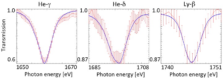
Figure 11: Model fits (blue) to the Mg He-$\gamma$, He-$\delta$, and Ly-$\beta$ lines recorded from experiment 2301 (red). The inferred conditions are $T_{e}=166\pm 2$ eV and $n_{e}=\left(6.3\pm 0.4\right)\times 10^{21}\mathrm{cm^{-3}}$.

IV.2 35 $\mu$m rear $\mathrm{CH}$ tamper

We performed only one experiment, z2363, using the 35 $\mu$m rear $\mathrm{CH}$ tamper target, whose spectra are shown in Fig. 10(b). The Fe:Mg atomic ratio is 0.9:1. The lines with $\tau_{\nu}<1$ are Mg He-$\gamma$ and Ly-$\beta$. These lines are simultaneously analyzed, and the fits are given in Fig. 12(a) and (b), respectively. The inferred conditions are $T_{e}=170\pm 2$ eV and $n_{e}=\left(2.0\pm 0.2\right)\times 10^{22}\,\mathrm{cm^{-3}}$. We confirmed a slight increase in $T_{e}$ and more than a factor of two increase in $n_{e}$ compared to the conditions achieved by the 10 $\mu$m rear $\mathrm{CH}$ tamper target. Since there is only one experiment from this target configuration, the uncertainties do not include experiment-to-experiment sample conditions reproducibility.

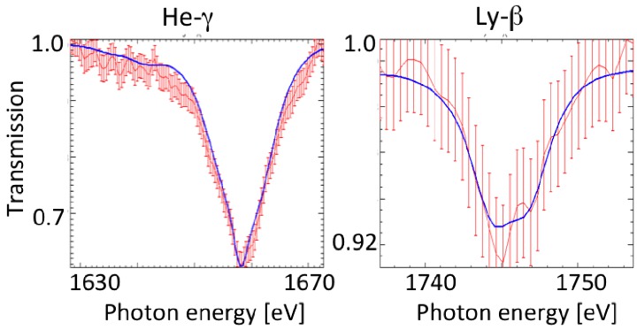
Figure 12: Mg He-$\gamma$ and Ly-$\beta$ are simultaneously fit for experiment z2363. The best fit is provided by $T_{e}=170$ eV and $n_{e}=2.0\times 10^{22}\,\mathrm{cm^{-3}}$.

IV.3 68 $\mu$m thick rear $\mathrm{CH}$ tamper

We performed six experiments using the 68 $\mu$m rear $\mathrm{CH}$ tamped target illustrated in Fig. 9(c). Mg lines with $\tau_{\nu}<$1 are He-$\gamma$, Ly-$\beta$, and the He-like satellite lines of Ly-$\alpha$. Thus, these lines from z2364 [i.e., Fig. 10(c)] are simultaneously analyzed using RADIATOR+GALM. The fits to these lines are shown in the Fig. 13, and the inferred conditions are $T_{e}=195\pm 3$ eV and $n_{e}=\left(4.3\pm 0.5\right)\times 10^{22}\,\mathrm{cm^{-3}}$.

While the $\mathrm{CH}$ configurations are the same for the six experiments, Fe areal number densities are different to test the reliability of the measured Fe opacity by applying Beer’s lawBailey et al. (2009). Figure 14 shows the conditions inferred for each of the six experiments in (a) $T_{e}$ and (b) $n_{e}$. Experiments z2364 and z2366 were performed with the thinnest Fe samples, whose areal densities were $\sim\mathrm{0.66\times 10^{18}\,Fe/cm^{2}}$ (atomic ratio of Fe:Mg=0.5:1). Experiments z2242 and z2270 were performed with intermediate Fe thicknesses with areal number densities of $\sim 1.2\times 10^{18}\,\mathrm{Fe/cm^{2}}$ (Fe:Mg=1:1). Experiments z2244 and z2267 were performed with the thickest Fe samples with areal number densities of $\sim\mathrm{2.9\times 10^{18}\,Fe/cm^{2}}$ (Fe:Mg=2.3:1). We did not observe any correlation between Fe thickness and the inferred Fe conditions. The average and standard deviation are indicated by blue solid and dashed lines, respectively: $T_{e}=196\pm 5$ eV and $n_{e}=\left(3.8\pm 0.5\right)\times 10^{22}\,\mathrm{cm^{-3}}$. Based on the standard deviations, the Fe condition reproducibility is $\pm$3% in $T_{e}$ and $\pm$13% in $n_{e}$. The mean individual measurement uncertainties are 3 eV and 0.6$\times\mathrm{10^{22}\,cm^{-3}}$. The total $T_{e}$ and $n_{e}$ uncertainties are computed by adding the experiment-to-experiment variations and the mean individual measurement uncertainties in quadrature, which are 6 eV ($\pm$3%) and $\mathrm{0.8\times 10^{22}\,cm^{-3}}$ ($\pm$21%), respectively.

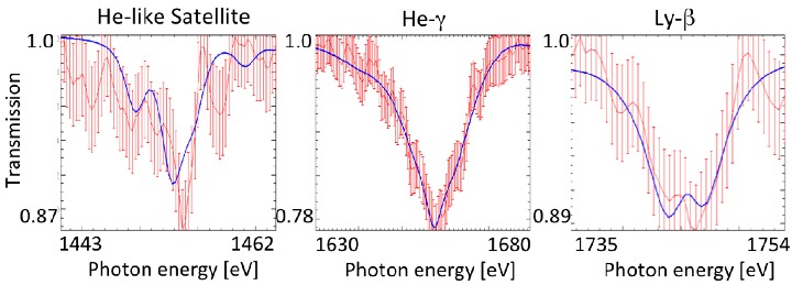
Figure 13: Fits to Mg He-like satellites, He-$\gamma$, and Ly-$\beta$ recorded on experiment z2364. The inferred conditions are $T_{e}=195\pm 3$ eV and $n_{e}=\left(4.3\pm 0.5\right)\times 10^{22}\,\mathrm{cm^{-3}}$.

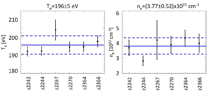
Figure 14: Fe condition analysis result summary for thick rear $\mathrm{CH}$ tamper targets. The average and standard deviation are indicated by blue solid and dashed lines, respectively: $T_{e}=196\pm 5$ eV and $n_{e}=\left(3.8\pm 0.5\right)\times 10^{22}\,\mathrm{cm^{-3}}$. The experiment-to-experiment variations of $T_{e}$ and $n_{e}$ over the six experiments are $\pm$3% and $\pm$13%, respectively.

V Uniformity measurement

Uniformity of the Fe sample is asserted based on volumetric heating provided by the powerful ZPDH radiation. In Sec. IV, similar Fe conditions are inferred from different Fe thicknesses, which also supports the sample axial uniformity. However, since volumetric heating is never perfect and heating radiation is supplied from one side, it is worthwhile to examine the axial uniformity assumption with more explicit experimental evidence. To this end, an experiment was designed to investigate the sample axial non-uniformity. Instead of mixing Mg throughout the Fe sample, Mg is mixed in the observer (rear) side of Fe and another dopant, Al (Z=13), is mixed in the radiation source (front) side of the Fe (Fig. 15), which are separated by a pure Fe region. One can infer Fe conditions in the radiation source side and in the observer side by Al and Mg K-shell spectroscopy, respectively.

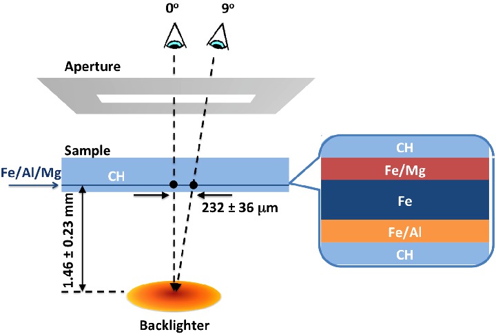
Figure 15: Spectrometers on axis and at 9^∘ sample transmission spectra from slightly different spatial centers. The analyses of the measured spectra would reveal not only axial non-uniformity but also a lateral gradient if it were significant.

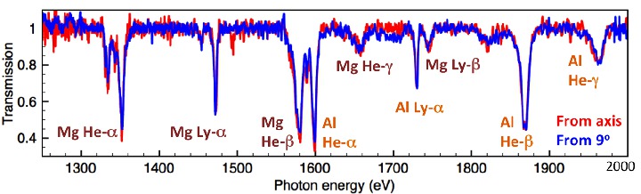
Figure 16: Comparison of line transmission spectra recorded along the vertical axis (at 0^∘) and at 9^∘. The good agreement indicates lateral gradients are insignificant.

The resultant Fe/Al/Mg (atomic ratio of 2:1:1) absorption spectra were recorded along two different lines of sight; one along the vertical axis (at 0^∘) and the other at 9^∘ from the vertical axis as in Fig. 15. The distance between the sample and the backlighter is measured on similar experiments, based on parallax, and found to be 1.5$\pm$0.2 mm. Due to this source-to-sample distance, when the spectrometers observe the backlighter through the Fe/Al/Mg sample, they see through slightly different spatial regions in the sample, which are separated by 232$\pm$36 $\mu$m as indicated in Fig. 15. The spectra are extracted by integrating the backlighter images over the central 300 $\mu$m. Since their backlighter centers appear at different points in the sample, which are separated by 236 $\mu$m, 300 $\mu$m integrations span different lateral regions in the sample with a small amount of overlap ($\sim$64 $\mu$m). Thus, in addition to measuring an axial gradient, these data will reveal a lateral gradient if it is significant. Figure 16 shows the extracted line transmission spectra. In addition to Mg, lines from Al are apparent.

The lines with $\tau_{\nu}<1$ are He-$\gamma$ and Ly-$\beta$ from Mg and Ly-$\alpha$ and He-$\gamma$ from Al. These spectra are analyzed using RADIATOR+GALM and the inferred $T_{e}$ and $n_{e}$ are summarized in Table 1. Figure 17 shows the resultant $T_{e}$ (left) and $n_{e}$ (right). Red and blue data points are the plasma conditions inferred for the radiation source side (Al mixed side) and the observer side (Mg mixed side) of the Fe sample, respectively. The red and the blue points agree within their measurement uncertainties. Thus, it is confirmed that there is no measurable axial gradient in the sample. Also, the conditions inferred from different spectrometers (i.e., 0^∘ and $9^{\circ}$) agree within their uncertainties. These results indicate that there is no gradient over $\pm 230\,\mu$m from the heating center (i.e., the point in the sample where the backlighter center appears from the spectrometer at $0^{\circ}$).

$0^{\circ}$	$T_{e}$ [eV]	$n_{e}$ [$\mathrm{10^{22}\,cm^{-3}}$]
Al side	$\mathrm{210\pm 3}$	$\mathrm{4.9\pm 1.2}$
Mg side	$\mathrm{211\pm 5}$	$\mathrm{4.0\pm 1.0}$

$9^{\circ}$	$T_{e}$ [eV]	$n_{e}$ [$\mathrm{10^{22}\,cm^{-3}}$]
Al side	$\mathrm{214\pm 2}$	$\mathrm{5.6\pm 1.0}$
Mg side	$\mathrm{211\pm 3}$	$\mathrm{5.2\pm 0.9}$

Table 1: Sample uniformity analysis results. No measurable axial nor lateral gradients are observed.

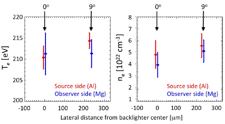
Figure 17: Measured $T_{e}$ (left) and $n_{e}$ (right) from uniformity analysis. The agreement between the conditions measured in the radiation source side (red) and observer side (blue) of the sample confirm that there is no axial gradient within uncertainties. Similarly, the agreement between the 0^∘ and $9^{\circ}$ line of sight conditions show that there is no measurable lateral gradient.

VI Conclusions

We addressed three of the key opacity measurement requirements: sample conditions control, independent sample condition measurements, and sample uniformity verification. The opacity experiments were performed at the Sandia National Laboratories Z-machine to benchmark opacity models for Fe at the base of solar convection zone where $T_{e}$ and $n_{e}$ are 185 eV and $\mathrm{9\times 10^{22}\,cm^{-3}}$, respectively. The Fe sample conditions were controlled by the tamping $\mathrm{CH}$ thicknesses. Increasing the rear $\mathrm{CH}$ thickness slows down the expansion, and the Fe samples remain dense at the time of backlighting. Three different rear $\mathrm{CH}$ thicknesses are tested: i) 10 $\mu$m, ii) 35 $\mu$m, and iii) 68 $\mu$m. The resultant Fe conditions are independently measured by Mg K-shell spectroscopy and found to be i) $T_{e}$=167$\pm 3$ eV and $n_{e}=\mathrm{\left(7.1\pm 1.5\right)\times 10^{21}\,cm^{-3}}$, ii) $T_{e}$=170$\pm 2$ eV and $n_{e}=\mathrm{\left(2.0\pm 0.2\right)\times 10^{22}\,cm^{-3}}$, and iii) $T_{e}$=196$\pm 6$ eV and $n_{e}=\mathrm{\left(3.8\pm 0.8\right)\times 10^{22}\,cm^{-3}}$, respectively. One experiment was designed and performed to specifically investigate the sample uniformity, with Al mixed into the side of the sample facing the radiation source (front), and Mg mixed in the opposite side of the sample (rear). The conditions at the bottom and the top of the Fe sample were inferred by Al and Mg K-shell spectroscopy, respectively, and confirmed that there are no measurable gradients in the sample. The inferred condition uncertainties due to K-shell spectral model details are under investigation, as well as the effects of non-LTE, sample self-emission, and temporal gradients. While different K-shell spectral models might infer slightly different $T_{e}$ and $n_{e}$, those differences should be systematic and would not affect the conclusions on the condition reproducibility and the sample uniformity. The sample condition uncertainties due to K-shell spectral model details are under investigation.

Fe opacity experiments at three different conditions with similar charge state distributions provide crucial information to disentangle complex physical processes in opacity models. Opacity models have to accurately compute relevant atomic data, atomic level populations, and then spectral formation, taking into account correct line shapes, and the complexity is enhanced as temperature and density increase. In LTE, the same average ionizations achieved by different $T_{e}$ and $n_{e}$ have different population distribution within each charge state because of the temperature dependence on the Boltzmann relationship [$p_{excited}/p_{ground}\propto\exp\left(-\Delta E/kT\right)$]. As temperature increases, more population is in excited states and absorption starting from those excited states becomes more important. Thus, at higher temperature, the accuracy and the treatment of excited states (i.e., singly-, doubly-, …, multiply-excited states) become more crucial to accurately solve for population and model opacity. As density increases, the effects of continuum lowering and Stark broadening become more important. Since our data are measured at different $T_{e}$ and $n_{e}$ with similar charge states, we can study how these effects gradually change the true opacity, and how well state-of-the-art opacity models can calculate them.

Appendix A: Extraction of local emissivity and opacity from PrismSPECT

PrismSPECT is a collisional radiative model that computes atomic level populations and then computes opacity (i.e., mass absorption coefficient), $\kappa_{\nu}^{mass}$, and emergent spectral radiance, $I_{\nu}$MacFarlane and al (2003); MacFarlane et al. (2007). In slab geometry, these two outputs are related by the following equations:

$$I_{\nu}=\frac{\epsilon_{\nu}}{\kappa_{\nu}}\left[1-\exp\left(-\kappa_{\nu}L\right)\right]$$ (8)

$$\kappa_{\nu}=\kappa_{\nu}^{mass}\rho$$ (9)

where $L$ is the thickness of the slab, and $\epsilon_{\nu}$ and $\kappa_{\nu}$ are emission coefficient (or $emissivity$) and absorption coefficient (or $opacity$), respectivelyMihalas (1978). For the rest of Appendix A and B, opacity refers to absorption coefficient, $\kappa_{\nu}$ (not mass absorption coefficient, $\kappa_{\nu}^{mass}$). Since both emissivity and opacity are proportional to the ion number density, $n_{ion}$, it is convenient to invert the PrismSPECT outputs, $I_{\nu}$ and $\kappa_{\nu}^{mass}$, into what we call fractional emissivity and opacity as follows:

$$\epsilon_{\nu}^{frac}\equiv\frac{\epsilon_{\nu}}{n_{ion}}=\frac{m_{ion}I_{\nu}\kappa_{\nu}^{mass}}{1-\exp\left(-\kappa_{\nu}^{mass}\rho L\right)}$$ (10)

$$\kappa_{\nu}^{frac}\equiv\frac{\kappa_{\nu}}{n_{ion}}=m_{ion}\kappa_{\nu}^{mass}$$ (11)

The quantities $\epsilon_{\nu}^{frac}$ and $\kappa_{\nu}^{frac}$ are proportional to the initial state fractional population of relevant radiative processes and depend only on $T_{e}$ and $n_{e}$ in the LTE assumption. The database of $\epsilon_{\nu}^{frac}\left(T_{e},\,n_{e}\right)$ and $\kappa_{\nu}^{frac}\left(T_{e},\,n_{e}\right)$ can be very useful for quick spectra calculations. One can build a PrismSPECT fractional emissivity and opacity database of an element $X$, $\epsilon_{\nu}^{frac,\,X}\left(T_{e},\,n_{e}\right)$ and $\kappa_{\nu}^{frac,\,X}\left(T_{e},\,n_{e}\right)$, by performing a single element, LTE PrismSPECT calculation for ranges of temperature and density and extracting $\epsilon_{\nu}^{frac}$ and $\kappa_{\nu}^{frac}$ from each condition using Eqs. (11) and (10).

We note that PrismSPECT requires ion number density, $n_{ion}$, as an input (not $n_{e}$). Thus, $n_{e}$ has to be extracted from the PrismSPECT output using $n_{e}=Z^{*}n_{ion}$, where $Z^{*}$ is the mean charge of the plasma. Interpolations are required both to build the database and to use the database. The required database grid spacing in $T_{e}$, $n_{e}$, and $h\nu$, and PrismSPECT calculation details depend on the required accuracy, and have to be carefully investigated for each application. The database used in this article is optimized for the emergent spectra accuracy, and temperature and density diagnostics. The spectra based on the database with linear interpolation agree with the spectra directly computed by PrismSPECT within 1%. The uncertainties in inferred $T_{e}$ and $n_{e}$ due to the use of the database and the linear interpolation are within 0.5 % and 1%, respectively. For Mg and Al database calculations, PrismSPECT employed tabulated Stark line shapes for their K-shell lines, which were computed in detail by MERLMancini et al. (1991).

The advantage of the database is speed and flexibility. Fractional emissivity and opacity of an element are dependent only on $T_{e}$ and $n_{e}$ and independent of surrounding species, its own ion number density, and geometry. Thus, once the database is extracted for each element, one can compute spectra for either single or multiple elements, uniform or non-uniform, emission or absorption by solving radiation transport for a given geometry, without re-running collisional radiative models. The database extraction is not exclusive to PrismSPECT; databases can be extracted from other collisional models. The accuracy of the database depends on the details of the collisional model used and the numerical details of the extraction scheme. The idea of the database can be extended for non-LTE as long as the non-LTE effects are independent of geometry such as for the optically-thin approximation or for non-LTE effects dominated by strong external radiation.

Appendix B: Slab radiation transport solver for a mixture

Once fractional emissivity and opacity databases are computed for each element $X$ [i.e., $\epsilon_{\nu}^{frac,\,X}\left(T_{e},\,n_{e}\right)$ and $\kappa_{\nu}^{frac,\,X}\left(T_{e},\,n_{e}\right)$ in Appendix A], one can solve the slab radiation transport equation to compute emergent spectra for any mixture and any gradient. Geometry can even be extended to arbitrary shapesNagayama et al. (2012a). Assume there is an M species plasma, which is discretized into N zones along the observation line of sight where zone N is closest to the observer. By assuming that an event is observed very far from the plasma, emergent spectra seen from the observer can be computed by the following equation:

$$I_{\nu}=I_{\nu,0}\exp(-\tau_{\nu})+I_{\nu,N}^{plasma}+F_{\nu}$$ (12)

where $I_{\nu,\,0}$ is the incident spectral irradiance (or backlighter), $\tau_{\nu}$ is the net optical depth of the plasma, $I_{\nu,\,N}^{plasma}$ is the plasma self-emission taking into account its self-absorption effect, and $F_{\nu}$ is a potential additional background. $I_{\nu,\,N}^{plasma}$ can be computed recursively as follows:

$$\mathrm{I_{\nu,\,i}^{plasma}=I_{\nu,\,i-1}^{plasma}\exp\left(-\tau_{\nu,\,i}\right)+\frac{\epsilon_{\nu,\,i}}{\kappa_{\nu,\,i}}\left[1-\exp\left(-\tau_{\nu,\,i}\right)\right]}$$ (13)

$$I_{\nu,\,1}^{plasma}=\frac{\epsilon_{\nu,\,1}}{\kappa_{\nu,\,1}}\left[1-\exp\left(-\tau_{\nu,\,1}\right)\right]$$ (14)

$$\epsilon_{\nu,\,i}=\sum_{j=1}^{M}N_{i}^{j}\epsilon_{\nu}^{frac,\,j}\left(T_{e,\,i},\,n_{e,\,i}\right)$$ (15)

$$\kappa_{\nu,\,i}=\sum_{j=1}^{M}N_{i}^{j}\kappa_{\nu}^{frac,\,j}\left(T_{e,\,i},\,n_{e,\,i}\right)$$ (16)

$$\eta_{\nu,\,i}=\epsilon_{\nu,\,i}L_{i}\text{ and }\tau_{\nu,\,i}=\kappa_{\nu,\,i}L_{i}$$ (17)

where $I_{\nu,\,i}^{plasma}$ is the emergent spectral irradiance at the end of zone $i$ of the discretized plasma, and $\epsilon_{\nu,\,i}$ and $\kappa_{\nu,\,i}$ are local emissivity and opacity (i.e., absorption coefficient) in zone $i$, respectively. The local emissivity and opacity at zone $i$ (i.e., $\epsilon_{\nu,\,i}$ and $\kappa_{\nu,\,i}$) can be computed by summing element emissivity, $N_{i}^{j}\epsilon_{\nu}^{frac,\,j}\left(T_{e,\,i},\,n_{e,\,i}\right)$, and opacity, $N_{i}^{j}\kappa_{\nu}^{frac,\,j}\left(T_{e,\,i},\,n_{e,\,i}\right)$, over all of the species in zone $i$, where $N_{i}^{j}$ are the ion number density of element $j$ at zone $i$, and $T_{e,\,i}$ and $n_{e,\,i}$ are electron temperature and density at zone $i$, respectively. By multiplying $\epsilon_{\nu,\,i}$ and $\kappa_{\nu,\,i}$ by the zone length, $L_{i}$, one can compute self-emission in the optically-thin approximation, $\eta_{\nu,\,i}$, and the optical depth, $\tau_{\nu,\,i}$, of zone $i$, respectively. Furthermore, $\eta_{\nu}=\sum_{i}\eta_{\nu,\,i}$ and $\tau_{\nu}=\sum_{i}\tau_{\nu,\,i}$ gives the net self-emission in optically-thin approximation and the net optical depth of the plasma, respectively.

This formula is general and works for either emission or absorption spectra. If the incident flux (or backlighter) is weaker than the sample self emission (i.e., $I_{\nu,\,0}<I_{\nu,\,N}^{plasma}$), Eq. (13) gives emission spectra. If the backlighter is brighter (i.e., $I_{\nu,\,0}>I_{\nu,\,N}^{plasma}$), this formula naturally produces absorption spectra. The measured spectra can be simulated by convolving $I_{\nu}$ with instrument spectral shape, $g\left(\nu-\nu^{\prime}\right)$, as follows:

$$I_{\nu}^{\star}=\int g\left(\nu-\nu^{\prime}\right)I_{\nu^{\prime}}d\nu^{\prime}$$

where $\int g(\nu-\nu^{\prime})d\nu^{\prime}=1$. The measured transmission spectra, $T_{\nu}^{\star}$, can be computed by dividing $I_{\nu}^{\star}$ by the convolved backlighter, $\int g\left(\nu-\nu^{\prime}\right)I_{\nu^{\prime},\,0}d\nu^{\prime}$.

There are two limiting cases of Eq. (13). For these limiting cases, $F_{\nu}$ is neglected for communication purposes. One limiting case is the optically-thin approximation for emission spectra (i.e., $\kappa_{\nu,\,i}=0$ and $B_{\nu}=0$). This approximation simplifies Eq. (13) to $I_{\nu}=\eta_{\nu}$. The other limiting case is pure transmission or the bright-backlighter approximation (i.e., $I_{\nu,\,0}\gg I_{\nu,\,N}^{plasma}$), which simplifies Eq. (13) to the following:

$$I_{\nu}=I_{\nu,\,0}\exp(-\tau_{\nu})$$

When the backlighter is not only bright but also spectrally smooth, one can approximate the instrumental broadening effect as follows:

$$T_{\nu}^{\star} = \frac{\int g\left(\nu-\nu^{\prime}\right)I_{\nu^{\prime}}d\nu^{\prime}}{\int g\left(\nu-\nu^{\prime}\right)I_{\nu^{\prime},\,0}d\nu^{\prime}}$$

$$\approx \frac{\int g\left(\nu-\nu^{\prime}\right)I_{\nu^{\prime}}d\nu^{\prime}}{I_{\nu,\,0}\int g\left(\nu-\nu^{\prime}\right)d\nu^{\prime}}$$

$$\approx \int g\left(\nu-\nu^{\prime}\right)\frac{I_{\nu^{\prime}}}{I_{\nu,\,0}}d\nu^{\prime}$$

$$\approx \int g\left(\nu-\nu^{\prime}\right)T_{\nu^{\prime}}d\nu^{\prime}$$

which is Eq. (4). This approximation is valid when $I_{\nu,\,0}$ changes slowly over the instrumental spectral shape, $g\left(\nu-\nu^{\prime}\right)$.

In our application, areal number densities of each element (i.e., Fe, Mg, and Al) are measured prior to the experiments using Rutherford backscattering (RBS). They can also be inferred by RADIATOR+GALM because of their sensitivities to the line depths. Thus, rewriting the $\epsilon_{\nu,\,i}$/$\kappa_{\nu,\,i}$, $\eta_{\nu,\,i}$, and $\tau_{\nu,\,i}$ in terms of element areal number density, $\left(N^{j}L\right)$, and fraction of the element areal number density in each zone $i$, $\alpha_{i}^{j}=\left(N_{i}^{j}L_{i}\right)/\left(N^{j}L\right)$, is also useful:

$$\frac{\epsilon_{\nu,\,i}}{\kappa_{\nu,\,i}}=\frac{\epsilon_{\nu,\,i}L_{i}}{\kappa_{\nu,\,i}L_{i}}=\frac{\eta_{\nu,\,i}}{\tau_{\nu,\,i}}$$

$$\eta_{\nu,\,i}=\sum_{j}\epsilon_{\nu,\,i}^{frac,\,j}\alpha_{i}^{j}\left(N^{j}L\right)$$

$$\tau_{\nu,\,i}=\sum_{j}\kappa_{\nu,\,i}^{frac,\,j}\alpha_{i}^{j}\left(N^{j}L\right)$$

where $\sum_{i}\alpha_{i}^{j}=1.0$. By assuming the fraction $\alpha_{i}^{j}$ is determined by the initial target designNagayama et al. (2012b), one can compute emergent spectra of multi-species plasmas just by providing $T_{e,\,i}$ and $n_{e,\,i}$ at each zone $i$. The areal number density of each element, $\left(N^{j}L\right)$, can either be provided by RBS measurements or extracted from the analysis.

References

- Bailey et al. (2009) J. E. Bailey, G. A. Rochau, R. C. Mancini, C. A. Iglesias, J. J. MacFarlane, I. E. Golovkin, C. Blancard, P. Cosse, and G. Faussurier, “Experimental investigation of opacity models for stellar interior, inertial fusion, and high energy density plasmas,” Physics of Plasmas 16, 058101 (2009).
- Cox (1980) A. N. Cox, “The Masses of Cepheids,” Annu. Rev. Astro. Astrophys. 18, 15 (1980).
- Iglesias et al. (1987) C. A. Iglesias, F. J. Rogers, and B. G. Wilson, “Reexamination of the metal contribution to astrophysical opacity,” ApJ 322, L45 (1987).
- Iglesias et al. (1990) C. A. Iglesias, F. J. Rogers, and B. G. Wilson, “Opacities for classical Cepheid models,” ApJ 360, 221 (1990).
- Rogers and Iglesias (1993) F. J. Rogers and C. A. Iglesias, “Equation of State and Opacity of Stellar Plasmas,” GONG 1992. Seismic Investigation of the Sun and Stars 42, 155 (1993).
- Asplund et al. (2005) M. Asplund, N. Grevesse, and A. J. Sauval, “The Solar Chemical Composition,” GONG 1992. Seismic Investigation of the Sun and Stars 336, 25 (2005).
- Basu and Antia (2008) S. Basu and H. M. Antia, “Helioseismology and solar abundances,” Physics Reports 457, 217 (2008).
- Asplund et al. (2009) M. Asplund, N. Grevesse, A. J. Sauval, and P. Scott, “The Chemical Composition of the Sun,” Annu. Rev. Astro. Astrophys. 47, 481 (2009).
- Basu and Antia (2013) S. Basu and H. M. Antia, “Revisiting the Issue of Solar Abundances,” J. Phys.: Conf. Ser. 440, 012017 (2013).
- Perry et al. (1996) T. Perry, P. Springer, D. Fields, D. Bach, F. Serduke, C. Iglesias, F. Rogers, J. Nash, M. Chen, B. Wilson, W. Goldstein, B. Rozsynai, R. Ward, J. Kilkenny, R. Doyas, L. Da Silva, C. Back, R. Cauble, S. Davidson, J. Foster, C. Smith, A. Bar-Shalom, and R. Lee, “Absorption experiments on x-ray-heated mid-Z constrained samples,” Phys. Rev. E 54, 5617 (1996).
- Davidson et al. (1988) S. J. Davidson, J. M. Foster, C. C. Smith, K. A. Warburton, and S. J. Rose, “Investigation of the opacity of hot, dense aluminum in the region of its K edge,” Appl. Phys. Lett. 52, 847 (1988).
- Perry et al. (1991) T. Perry, S. Davidson, F. Serduke, D. Bach, C. Smith, J. Foster, R. Doyas, R. Ward, C. Iglesias, F. Rogers, J. Abdallah, R. Stewart, J. Kilkenny, and R. Lee, “Opacity measurements in a hot dense medium,” Physical Review Letters 67, 3784 (1991).
- Foster et al. (1991) J. Foster, D. Hoarty, C. Smith, P. Rosen, S. Davidson, S. Rose, T. Perry, and F. Serduke, “L-shell absorption spectrum of an open-M-shell germanium plasma: Comparison of experimental data with a detailed configuration-accounting calculation,” Physical Review Letters 67, 3255 (1991).
- Chenais-Popovics et al. (2001) C. Chenais-Popovics, M. Fajardo, F. Gilleron, U. Teubner, J. C. Gauthier, C. Bauche-Arnoult, A. Bachelier, J. Bauche, T. Blenski, F. Thais, F. Perrot, A. Benuzzi, S. Turck-Chieze, J. P. Chièze, F. Dorchies, U. Andiel, W. Foelsner, and K. Eidmann, “L-band x-ray absorption of radiatively heated nickel,” Phys. Rev. E 65, 016413 (2001).
- Bailey et al. (2003) J. E. Bailey, P. Arnault, T. Blenski, G. Dejonghe, O. Peyrusse, J. J. MacFarlane, R. C. Mancini, M. E. Cuneo, D. S. Nielsen, and G. A. Rochau, “Opacity measurements of tamped NaBr samples heated by z-pinch X-rays,” Journal of Quantitative Spectroscopy and Radiative Transfer 81, 31 (2003).
- Renaudin et al. (2006) P. Renaudin, C. Blancard, J. Bruneau, G. Faussurier, J. E. Fuchs, and S. Gary, “Absorption experiments on X-ray-heated magnesium and germanium constrained samples,” Journal of Quantitative Spectroscopy and Radiative Transfer 99, 511 (2006).
- Da Silva et al. (1992) L. Da Silva, B. MacGowan, D. Kania, B. Hammel, C. Back, E. Hsieh, R. Doyas, C. Iglesias, F. Rogers, and R. Lee, “Absorption measurements demonstrating the importance of n=0 transitions in the opacity of iron,” Physical Review Letters 69, 438 (1992).
- Springer et al. (1992) P. Springer, D. Fields, B. Wilson, J. Nash, W. Goldstein, C. Iglesias, F. Rogers, J. Swenson, M. Chen, A. Bar-Shalom, and R. Stewart, “Spectroscopic absorption measurements of an iron plasma,” Physical Review Letters 69, 3735 (1992).
- Winhart et al. (1995) G. Winhart, K. Eidmann, C. A. Iglesias, A. Bar-Shalom, E. Mínguez, A. Rickert, and S. J. Rose, “XUV opacity measurements and comparison with models,” Journal of Quantitative Spectroscopy and Radiative Transfer 54, 437 (1995).
- Springer et al. (1997) P. T. Springer, K. L. Wong, C. A. Iglesias, J. H. Hammer, J. L. Porter, A. Toor, W. H. Goldstein, B. G. Wilson, F. J. Rogers, C. Deeney, D. S. Dearborn, C. Bruns, J. Emig, and R. E. Stewart, “Laboratory measurement of opacity for stellar envelopes,” Journal of Quantitative Spectroscopy and Radiative Transfer 58, 927 (1997).
- Chenais Popovics et al. (2000) C. Chenais Popovics, H. Merdji, T. Missalla, F. Gilleron, J. C. Gauthier, T. Blenski, F. Perrot, M. Klapisch, C. Bauche-Arnoult, J. Bauche, A. Bachelier, and K. Eidmann, “Opacity Studies of Iron in the 15–30eV Temperature Range,” ApJS 127, 275 (2000).
- Iglesias (2006) C. A. Iglesias, “Effects of Backlight Structure on Absorption Experiments,” Journal of Quantitative Spectroscopy and Radiative Transfer 99, 295 (2006).
- Bailey et al. (2007) J. Bailey, G. Rochau, C. Iglesias, J. Abdallah, J. MacFarlane, I. Golovkin, P. Wang, R. Mancini, P. Lake, T. Moore, M. Bump, O. Garcia, and S. Mazevet, “Iron-Plasma Transmission Measurements at Temperatures Above 150 eV,” Physical Review Letters 99 (2007).
- Griem (1968) H. Griem, “Semiempirical Formulas for the Electron-Impact Widths and Shifts of Isolated Ion Lines in Plasmas,” Phys. Rev. 165, 258 (1968).
- Nash et al. (2010) T. J. Nash, G. A. Rochau, and J. E. Bailey, “Design of dynamic Hohlraum opacity samples to increase measured sample density on Z,” Rev. Sci. Instrum. 81, 10E518 (2010).
- Bailey et al. (2006) J. E. Bailey, G. A. Chandler, R. C. Mancini, S. A. Slutz, G. A. Rochau, M. Bump, T. J. Buris-Mog, G. Cooper, G. Dunham, I. Golovkin, J. D. Kilkenny, P. W. Lake, R. J. Leeper, R. Lemke, J. J. MacFarlane, T. A. Mehlhorn, T. C. Moore, T. J. Nash, A. Nikroo, D. S. Nielsen, K. L. Peterson, C. L. Ruiz, D. G. Schroen, D. Steinman, and W. Varnum, “Dynamic hohlraum radiation hydrodynamics,” Physics of Plasmas 13, 056301 (2006).
- (27) G. A. Rochau, J. E. Bailey, R. E. Falcon, G. Loisel, T. Nagayama, B. T. Hutsel, R. C. Mancini, I. Hall, D. E. Winget, M. H. Montgomery, and D. A. Liedahl, “ZAPP: The Z Astrophysical Plasma Properties collaboration,” Submitted to Physics of Plasmas .
- Henke et al. (1984a) B. L. Henke, S. L. Kwok, J. Y. Uejio, H. T. Yamada, and G. C. Young, “Low-energy x-ray response of photographic films I Mathematical models,” J. Opt. Soc. Am. B 1, 818 (1984a).
- Henke et al. (1984b) B. L. Henke, F. G. Fujiwara, M. A. Tester, C. H. Dittmore, and M. A. Palmer, “Low-energy x-ray response of photographic films II Experimental characterization,” J. Opt. Soc. Am. B 1, 828 (1984b).
- Griem (1992) H. R. Griem, “Plasma spectroscopy in inertial confinement fusion and soft x-ray laser research,” Physics of Fluids B: Plasma Physics 4, 2346 (1992).
- Hammel et al. (1993) B. A. Hammel, C. J. Keane, M. D. Cable, D. R. Kania, J. D. Kilkenny, R. W. Lee, and R. Pasha, “X-ray spectroscopic measurements of high densities and temperatures from indirectly driven inertial confinement fusion capsules,” Physical Review Letters 70, 1263 (1993).
- Bailey et al. (2004) J. E. Bailey, G. A. Chandler, S. A. Slutz, I. Golovkin, P. W. Lake, J. J. MacFarlane, R. C. Mancini, T. J. Burris-Mog, G. Cooper, R. J. Leeper, T. A. Mehlhorn, T. C. Moore, T. J. Nash, D. S. Nielsen, C. L. Ruiz, D. G. Schroen, and W. A. Varnum, “Hot Dense Capsule-Implosion Cores Produced by Z-Pinch Dynamic Hohlraum Radiation,” Physical Review Letters 92, 085002 (2004).
- Bailey et al. (2008) J. E. Bailey, G. A. Rochau, R. C. Mancini, C. A. Iglesias, J. J. MacFarlane, I. E. Golovkin, J. C. Pain, F. Gilleron, C. Blancard, P. Cosse, G. Faussurier, G. A. Chandler, T. J. Nash, D. S. Nielsen, and P. W. Lake, “Diagnosis of x-ray heated Mg/Fe opacity research plasmas,” Rev. Sci. Instrum. 79, 113104 (2008).
- Kramida et al. (2013) A. Kramida, Y. Ralchenko, J. Reader, and NIST ASD Team, NIST Atomic Spectra Database (ver. 5.1), [Online], Tech. Rep. (2013).
- Baranger (1958) M. Baranger, “General Impact Theory of Pressure Broadening,” Phys. Rev. 112, 855 (1958).
- Smith (1966) E. W. Smith, A relaxation theory of spectral line broadening in plasmas, Ph.D. thesis, University of Florida, University of Florida (1966).
- Griem (1974) H. Griem, Spectral line broadening by plasmas, Pure and Applied Physics Series (New York ; London : Academic Press, 1974).
- Tighe and Hooper (1978) R. Tighe and C. Hooper, “Stark broadening in hot, dense, laser-produced plasmas: A two-component, two-temperature formulation,” Phys. Rev. A 17, 410 (1978).
- Mancini et al. (1991) R. C. Mancini, D. P. Kilcrease, L. A. Woltz, and C. F. Hooper, Jr., “Calculational aspects of the Stark line broadening of multielectron ions in plasmas,” Computer Physics Communications 63, 314 (1991).
- Alexiou (2009) S. Alexiou, “Overview of plasma line broadening,” High Energ Dens Phys 5, 225 (2009).
- Iglesias and Sonnad (2010) C. A. Iglesias and V. Sonnad, “Robust algorithm for computing quasi-static stark broadening of spectral lines,” High Energ Dens Phys 6, 399 (2010).
- Stambulchik and Maron (2010) E. Stambulchik and Y. Maron, “Plasma line broadening and computer simulations: A mini-review,” High Energ Dens Phys 6, 9 (2010).
- MacFarlane and al (2003) J. J. MacFarlane and e. al, “Simulation of the Ionization Dynamics of Aluminum Irradiated by Intense Short-Pulse Lasers,” in International Symposium on Inertial Fusion Science and Applications 2003 (2003) p. 457.
- MacFarlane et al. (2007) J. J. MacFarlane, I. E. Golovkin, P. Wang, P. R. Woodruff, and N. A. Pereyra, “SPECT3D – A multi-dimensional collisional-radiative code for generating diagnostic signatures based on hydrodynamics and PIC simulation output,” High Energ Dens Phys 3, 181 (2007).
- Nagayama et al. (2012a) T. Nagayama, R. C. Mancini, R. Florido, D. Mayes, R. Tommasini, J. A. Koch, J. A. Delettrez, S. P. Regan, and V. A. Smalyuk, “Investigation of a polychromatic tomography method for the extraction of the three-dimensional spatial structure of implosion core plasmas,” Physics of Plasmas 19, 082705 (2012a).
- Goldberg (1989) D. E. Goldberg, Genetic Algorithms in Search, Optimization and Machine Learning, 1st ed. (Addison-Wesley Longman Publishing Co., Inc., Boston, MA, USA, 1989).
- Press et al. (1992) W. H. Press, S. A. Teukolsky, W. T. Vetterling, and B. P. Flannery, Numerical Recipes in C: The Art of Scientific Computing, 2nd ed. (Cambridge University Press, New York, NY, USA, 1992).
- Hansen et al. (2007) S. Hansen, J. Bauche, C. BAUCHEARNOULT, and M. GU, “Hybrid atomic models for spectroscopic plasma diagnostics,” High Energ Dens Phys 3, 109 (2007).
- Florido et al. (2009) R. Florido, R. Rodríguez, J. M. Gil, J. G. Rubiano, P. Martel, E. Mínguez, and R. C. Mancini, “Modeling of population kinetics of plasmas that are not in local thermodynamic equilibrium, using a versatile collisional-radiative model based on analytical rates,” Phys. Rev. E 80, 56402 (2009).
- Iglesias et al. (1985) C. Iglesias, H. DeWitt, J. Lebowitz, D. MacGowan, and W. Hubbard, “Low-frequency electric microfield distributions in plasmas,” Phys. Rev. A 31, 1698 (1985).
- Loisel et al. (2012) G. Loisel, J. E. Bailey, G. A. Rochau, G. S. Dunham, L. B. Nielsen-Weber, and C. R. Ball, “A methodology for calibrating wavelength dependent spectral resolution for crystal spectrometers,” Rev. Sci. Instrum. 83, 10E133 (2012).
- Chenais-Popovics et al. (1990) C. Chenais-Popovics, C. Fievet, J. P. Geindre, I. Matsushima, and J. C. Gauthier, “Saturation effects in K absorption spectroscopy of laser-produced plasmas,” Physical Review A (Atomic 42, 4788 (1990).
- Zimmerman et al. (1978) G. Zimmerman, D. Kershaw, D. Bailey, and J. Harte, “LASNEX code for inertial confinement fusion (A),” Journal of the Optical Society of America (1917-1983) 68, 549 (1978).
- Mihalas (1978) D. Mihalas, Stellar Atmospheres, A Series of books in astronomy and astrophysics (W. H. Freeman, 1978).
- Nagayama et al. (2012b) T. Nagayama, J. E. Bailey, G. A. Rochau, S. B. Hansen, R. C. Mancini, J. J. MacFarlane, and I. Golovkin, “Investigation of iron opacity experiment plasma gradients with synthetic data analyses,” Rev. Sci. Instrum. 83, 10E128 (2012b).