The $L-\sigma$ relation for massive bursts of star formation

Abstract

The validity of the emission line luminosity vs. ionised gas velocity dispersion ($L-\sigma$) correlation for HII galaxies (HIIGx), and its potential as an accurate distance estimator are assessed.

For a sample of 128 local ($0.02\lesssim z\lesssim 0.2$) compact HIIGx with high equivalent widths of their Balmer emission lines we obtained ionized gas velocity dispersion from high S/N high-dispersion spectroscopy (Subaru-HDS and ESO VLT-UVES) and integrated H$\beta$ fluxes from low dispersion wide aperture spectrophotometry.

We find that the $L(\mathrm{H}\beta)-\sigma$ relation is strong and stable against restrictions in the sample (mostly based on the emission line profiles). The ‘gaussianity’ of the profile is important for reducing the rms uncertainty of the distance indicator, but at the expense of substantially reducing the sample.

By fitting other physical parameters into the correlation we are able to significantly decrease the scatter without reducing the sample. The size of the starforming region is an important second parameter, while adding the emission line equivalent width or the continuum colour and metallicity, produces the solution with the smallest rms scatter=$\delta\log L(\mathrm{H}\beta)=0.233$.

The derived coefficients in the best $L(\mathrm{H}\beta)-\sigma$ relation are very close to what is expected from virialized ionizing clusters, while the derived sum of the stellar and ionised gas masses are similar to the dynamical mass estimated using the HST corrected Petrosian radius. These results are compatible with gravity being the main mechanism causing the broadening of the emission lines in these very young and massive clusters. The derived masses range from about 2 $\times 10^{6}$ M_⊙ to $10^{9}$ M_⊙  and their ‘corrected’ Petrosian radius, from a few tens to a few hundred parsecs.

1 Introduction

Observational cosmology has witnessed in the last few years advances that resulted in the inception of what many consider the first precision cosmological model, involving a spatially flat geometry and an accelerated expansion of the Universe. To build a robust model of the Universe it is necessary not only to set the strongest possible constraints on the cosmological parameters, applying joint analyses of a variety of distinct methodologies, but also to confirm the results through extensive consistency checks, using independent measurements and different methods, in order to identify and remove possible systematic errors, related to either the methods themselves or the tracers used.

It is accepted that young massive star clusters, like those responsible for the ionisation in giant extragalactic HII regions (GEHR) and HII galaxies (HIIGx) display a correlation between the luminosity and the width of their emission lines, the $L(\mathrm{H}\beta)-\sigma$ relation (Terlevich & Melnick, 1981). The scatter in the relation is small enough that it can be used to determine cosmic distances independently of redshift (Melnick et al., 1987; Melnick et al., 1988; Siegel et al., 2005; Bordalo & Telles, 2011; Plionis et al., 2011; Chávez et al., 2012). Melnick et al. (1988) used this correlation to determine $H_{0}=89\pm 10$ km s^-1Mpc^-1 and Chávez et al. (2012), using a subset of the sample of HIIGx that we will present in this work, found a value for $H_{0}=74.3\pm 3.1{\rm(random)}\pm 2.9{\rm(systematic)}$ km s^-1Mpc^-1, which is consistent with, and independently confirms, the Riess et al. (2011, $H_{0}=73.8\pm 2.4$ km s^-1Mpc^-1) and more recent SNIa results (e.g.  Freedman et al., 2012, $H_{0}=74.3\pm 1.5\pm 2.1$ km s^-1Mpc^-1).

GEHR are massive bursts of star formation generally located in the outer disk of late type galaxies. HIIGx are also massive bursts of star formation but in this case located in dwarf irregular galaxies and almost completely dominating the total luminosity output. The optical spectra of both GEHR and HIIGx, indistinguishable from each other, are characterized by strong emission lines produced by the gas ionized by a young massive star cluster (Searle & Sargent, 1972; Bergeron, 1977; Terlevich & Melnick, 1981; Kunth & Östlin, 2000). One important property is that, as the mass of the young stellar cluster increases, both the number of ionizing photons and the motion of the ionised gas, which is determined by the gravitational potential of the stellar cluster and gas complex, also increases. This fact induces the correlation between the luminosity of recombination lines, e.g. $L(\mathrm{H}\beta)$, which is proportional to the number of ionizing photons, and the ionized gas velocity dispersion ($\sigma$), which can be measured using the emission lines width as an indicator.

Recently Bordalo & Telles (2011) have explored the $L(\mathrm{H}\alpha)-\sigma$ correlation and its systematic errors using a nearby sample selected from the Terlevich et al. (1991) spectrophotometric catalogue of HIIGx ($0\lesssim z\lesssim 0.08$). They conclude that considering only the objects with clearly gaussian profiles in their emission lines, they obtain something close to an $L(\mathrm{H}\alpha)\propto\sigma^{4}$ relation with an rms scatter of $\delta\log L(\mathrm{H}\alpha)\sim 0.30$. It is important to emphasise that the observed properties of HIIGx, in particular the derived $L(\mathrm{H}\beta)-\sigma$  relation, are mostly those of the young burst and not those of the parent galaxy. This is particularly true if one selects those systems with the largest equivalent width (EW) in their emission lines, i.e. EW(H$\beta)>50$Å  as we will discuss in the body of the paper. The selection of those HIIGx having the strongest emission lines minimises the evolutionary effects in their luminosity (Copetti, Pastoriza & Dottori, 1986), which would introduce a systematic shift in the $L(\mathrm{H}\beta)-\sigma$ relation due to the rapid drop of the ionising flux after 5 Myr of evolution. This selection minimises also any possible contamination in the observable due to the stellar populations of the parent galaxy.

A feature of the HIIGx optical spectrum, their strong and narrow emission lines, makes them readily observable with present instrumentation out to $z\sim 3.5$. Regarding such distant systems, Koo et al. (1995) and also Guzmán et al. (1996) have shown that a large fraction of the numerous compact star forming galaxies found at intermediate redshifts have kinematical properties similar to those of luminous local HIIGx. They exhibit fairly narrow emission line widths ($\sigma$ from 30 to 150 km/s) rather than the 200 km/s typical for galaxies of similar luminosities. In particular galaxies with $\sigma<$ 65 km/s seem to follow the same relations in $\sigma$, M_B and $L(\mathrm{H}\beta)$ as the local ones.

From spectroscopy of Balmer emission lines in a few Lyman break galaxies at $z\sim$ 3 Pettini et al. (1998) suggested that these systems adhere to the same relations but that the conclusions had to be confirmed for a larger sample. These results opened the important possibility of applying the distance estimator and mapping the Hubble flow up to extremely high redshifts and simultaneously to study the behaviour of starbursts of similar luminosities over a very large redshift range.

Using a sample of intermediate and high redshift HIIGx Melnick, Terlevich & Terlevich (2000) investigated the use of the $L(\mathrm{H}\beta)-\sigma$ correlation as a high-$z$ distance indicator. They found a good correlation between the luminosity and velocity dispersion confirming that the $L(\mathrm{H}\beta)-\sigma$  correlation for local HIIGx is valid up to $z\sim$3. Indeed, our group (Plionis et al., 2011) showed that the HIIGx $L(\mathrm{H}\beta)-\sigma$ relation constitutes a viable alternative cosmic probe to SNe Ia. We also presented a general strategy to use HIIGx to trace the high-$z$ Hubble expansion in order to put stringent constrains on the dark energy equation of state and test its possible evolution with redshift. A first attempt by Siegel et al. (2005), using a sample of 15 high-$z$ HIIGx ($2.1<z<3.4$), selected as in Melnick et al. (2000), with the original $L(\mathrm{H}\beta)-\sigma$ calibration of Melnick et al. (1988), found a mass content of the universe of $\Omega_{m}=0.21_{-0.12}^{+0.30}$ for a flat $\Lambda$-dominated universe. Our recent reanalysis of the Siegel et al. (2005) sample (Plionis et al., 2011), using a revised zero-point of the original $L(H\beta)-\sigma$ relation, provided a similar value of $\Omega_{m}=0.22^{+0.06}_{-0.04}$ but with substantially smaller errors (see also Jarosik et al., 2011).

Recapitulating, we reassess in this paper the HIIGx $L(\mathrm{H}\beta)-\sigma$ relation using new data obtained with modern instrumentation with the aim of reducing the impact of observational random and systematic errors onto the HIIGx Hubble diagram. To achieve this goal, we selected from the SDSS catalogue a sample of 128 local ($z<0.2$), compact HIIGx with the highest equivalent width of their Balmer emission lines. We obtained high S/N high-dispersion echelle spectroscopic data with the VLT and Subaru telescopes to accurately measure the ionized gas velocity dispersion. We also obtained integrated H$\beta$ fluxes using low dispersion wide aperture spectrophotometry from the 2.1m telescopes at Cananea and San Pedro Mártir in Mexico, complemented with data from the SDSS spectroscopic survey.

The layout of the paper is as follows: we describe the sample selection procedure in §2, observations and data reduction in §3; an analysis in depth of the data error budget (observational and systematic) and the method for analysing the data are discussed in §4. The effect that different intrinsic physical parameters of the star-forming regions could have on the $L(\mathrm{H}\beta)-\sigma$  relation is studied in §5. The results for the $L(\mathrm{H}\beta)-\sigma$ relation is presented in §6, together with possible second parameters and systematic effects. Summary and conclusions are given in §7. Fittings to the $\mathrm{H}\beta$ line profiles are shown in the Appendix which is available electronically.

2 Sample selection

We observed 128 HIIGx selected from the SDSS DR7 spectroscopic catalogue (Abazajian et al., 2009) for having the strongest emission lines relative to the continuum (i.e. largest equivalent widths) and in the redshift range $0.01<z<0.2$. The lower redshift limit was selected to avoid nearby objects that are more affected by local peculiar motions relative to the Hubble flow and the upper limit was set to minimize the cosmological non-linearity effects. Figure 1 shows the redshift distribution for the sample. The median of the distribution is also shown as a dashed line at $z\sim 0.045$, the corresponding recession velocity is $\sim 13500\ \mathrm{km\ s^{-1}}$.

Only those HIIGx with the largest equivalent width in their $\mathrm{H}\beta$ emission lines, $EW(\mathrm{H}\beta)>50\ \mathrm{\AA}$ were included in the sample. This relatively high lower limit in the observed equivalent width of the recombination hydrogen lines is of fundamental importance to guarantee that the sample is composed by systems in which a single very young starburst dominates the total luminosity. This selection criterion also minimizes the posible contamination due to an underlying older population or older clusters inside the spectrograph aperture [cf. Melnick et al. (2000); Dottori (1981); Dottori & Bica (1981)]. Figure 2 shows the $EW(\mathrm{H}\beta)$ distribution for the sample; the dashed line marks the median of the distribution, its value is $EW(\mathrm{H}\beta)\sim 87\ \mathrm{\AA}$.

Starbusrt99 (Leitherer et al., 1999, SB99) models indicate that an instantaneous burst with $EW(\mathrm{H}\beta)>50\ \mathrm{\AA}$ and Salpeter IMF has to be younger than about 5 Myr (see Figure 3). This is a strong upper limit because in the case that part of the continuum is produced by an underlying older stellar population, the derived cluster age will be even smaller.

Figure 1: Redshift distribution of the sample. The dashed line marks the median.

Figure 2: $\mathrm{H}\beta$ equivalent width distribution for the sample. The dashed line marks the median.

Figure 3: The evolution of the $\mathrm{H}\beta$ equivalent width for an instantaneous burst with metallicity Z$=0.004$ and a Salpeter IMF with upper limit of 100 M_⊙ (Leitherer et al., 1999). The horizontal line marks the $\mathrm{H}\beta$ equivalent width of 50 Å, while the vertical line indicates the corresponding age of $\sim$ 5 Myrs.

The sample is also flux limited as it was selected from SDSS for having an $\mathrm{H}\beta$ line core $\mathrm{h_{c}}(\mathrm{H}\beta)>100\times 10^{-17}\ \mathrm{erg\ s^{-1}cm^{-2}\AA^{-1}}$. To discriminate against high velocity dispersion objects and also to avoid those that are dominated by rotation, we have selected only those objects with $0.7<\sigma(\mathrm{H}\beta)<2.0\ \mathrm{\AA}$. From the values of the line core and $\sigma$ of the $\mathrm{H}\beta$ line we can calculate that the flux limit in the $\mathrm{H}\beta$ line is $F_{lim}(\mathrm{H}\beta)\sim 5\times 10^{-15}\ \mathrm{erg\ s^{-1}\ cm^{-2}}$ which corresponds to an emission-free continuum magnitude of $m_{B,lim}\simeq 19.2$ [cf. Terlevich & Melnick (1981) for the conversion].

To guarantee the best integrated spectrophotometry, only objects with Petrosian diameter less than 6″ were selected. In addition a visual inspection of the SDSS images was performed to avoid systems composed of multiple knots or extended haloes. Colour images from SDSS for a subset of objects in the sample are shown in Figure 4. The range in colour is related to the redshifts span of the objects and is due mainly to the dominant [OIII]$\lambda\lambda$4959,5007 doublet moving from the g to the r SDSS filters and to the RGB colour definition. The compactness of the sources can be appreciated in the figure.

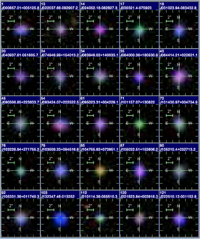
Figure 4: A selection of colour images of HIIGx from our sample. The SDSS name and our index number are indicated in the stamps. The changes in colour are related to the redshift of the object

3 Observations and Data Reduction

The data required for determining the $L(\mathrm{H}\beta)-\sigma$ relation are of two kinds:

1. Wide slit low resolution spectrophotometry to obtain accurate integrated emission line fluxes.

2. High resolution spectroscopy to measure the velocity dispersion from the $\rm{H}\beta$ and [OIII] line profiles. Typical values of the FWHM range from 30 to about 200$\ \rm{km\ s^{-1}}$.

A journal of observations is given in table 1 where column (1) gives the observing date, column (2) the telescope, column (3) the instrument used, column (4) the detector and column (5) the projected slit width in arc seconds.

Table 1: Journal of observations.

(1)	(2)	(3)	(4)	(5)
Dates	Telescope	Instrument	Detector	Slit-width
5 & 16 Nov 2008	NOAJ-Subaru	HDS	EEV (2 $\times$ 2K $\times$ 4K)	4′′
16 & 17 Apr 2009	ESO-VLT	UVES-Red	EEV (2 $\times$ 2K $\times$ 4K)	2′′
15 - 17 Mar 2010	OAN - 2.12m	B&C	SITe3 (1K $\times$ 1K)	10′′
10 - 13 Apr 2010	OAGH - 2.12m	B&C	VersArray (1300 $\times$ 660)	8.14′′
8 -10 Oct 2010	OAN - 2.12m	B&C	Thompson 2K	13.03′′
7 - 11 Dic 2010	OAGH - 2.12m	B&C	VersArray (1300 $\times$ 660)	8.14′′
4 - 6 Mar 2011	OAN - 2.12m	B&C	Thompson 2K	13.03′′
1 - 4 Apr 2011	OAGH - 2.12m	B&C	VersArray (1300 $\times$ 660)	8.14′′

3.1 Low resolution spectroscopy

The low resolution spectroscopy was performed with two identical Boller & Chivens Cassegrain spectrographs (B&C) in long slit mode at similar 2 meter class telescopes, one of them at the Observatorio Astronómico Nacional (OAN) in San Pedro Mártir (Baja California) and the other one at the Observatorio Astrofísico Guillermo Haro (OAGH) in Cananea (Sonora) both in México.

The observations at OAN were performed using a $600\ \mathrm{gr\ mm^{-1}}$ grating with a blaze angle of $8^{\circ}38^{\prime}$. The grating was centred at $\lambda\sim 5850\mathrm{\AA}$ and the slit width was 10″. The resolution obtained with this configuration is $R\sim 350$ ($\sim$ 2.07 Å/ pix) and the spectral coverage is $\sim 2100\ \mathrm{\AA}$. The data from OAGH was obtained using a $150\ \mathrm{gr\ mm^{-1}}$ grating with a blaze angle of $3^{\circ}30^{\prime}$ centred at $\lambda\sim 5000\mathrm{\AA}$. With this configuration and a slit width of 8.14″, the spectral resolution is $R\sim 83$ ($\sim$ 7.88 Å/ pix).

At least four observations of three spectrophotometric standard stars were performed each night. Futhermore, to secure the photometric link between different nights at least one HIIGx was repeated every night during each run. All objects were observed at small zenith distance, but for optimal determination of the atmospheric extinction the first and the last standard stars of the night were also observed at high zenith distance.

The wide-slit spectra obtained at OAN and OAGH were reduced using standard IRAF tasks. The reduction procedure entailed the following steps: (1) bias, flat field and cosmetic corrections, (2) wavelength calibration, (3) background subtraction, (4) flux calibration and (5) 1d spectrum extraction. The spectrophotometric standard stars for each night were selected among $\mathrm{G191-B2B}$, Feige 66, Hz 44, $\mathrm{BD+33d2642}$, GD 50, Hiltner 600, HR 3454, Feige 34 and GD 108.

We complemented our own wide-slit spectrophotometric observations with the SDSS DR7 spectroscopic data when available. SLOAN spectra are obtained with 3″diameter fibers, covering a range from $3200-9200\ \mathrm{\AA}$ and a resolution $R$ of $1850-2200$. The comparison between our own and SDSS spectrophotometry is discussed later on in §4.1.

3.2 High resolution spectroscopy

High spectral resolution spectroscopy was obtained using echelle spectrographs at 8 meter class telescopes. The telescopes and instruments used are the Ultraviolet and Visual Echelle Spectrograph (UVES) at the European Southern Observatory (ESO) Very Large Telescope (VLT) in Paranal, Chile, and the High Dispersion Spectrograph (HDS) at the National Astronomical Observatory of Japan (NAOJ) Subaru Telescope in Mauna Kea, Hawaii (see Table 1 for the journal of observations).

UVES is a two-arm cross-disperser echelle spectrograph located at the Nasmyth B focus of ESO-VLT Unit Telescope 2 (UT2; Kueyen) (Dekker et al., 2000). The spectral range goes from $3000\ \mathrm{\AA}$ to $11000\ \mathrm{\AA}$. The maximum spectral resolution is $80000$ and $110000$ in the blue and red arm respectively. We used the red arm ($31.6\ \mathrm{gr\ mm^{-1}}$ grating, $75.04^{\circ}$ blaze angle) with cross disperser 3 configuration ($600\ \mathrm{gr\ mm^{-1}}$ grating) centred at $5800\ \mathrm{\AA}$. The width of the slit was 2″, giving a spectral resolution of $\sim 22500$ (0.014 Å/pix).

HDS is a high resolution cross-disperser echelle spectrograph located at the optical Nasmyth platform of NAOJ-Subaru Telescope (Noguchi et al., 2002; Sato et al., 2002). The instrument covers from $3000\ \mathrm{\AA}$ to $10000\ \mathrm{\AA}$. The maximum spectral resolution is $160000$. The echelle grating used has $31.6\ \mathrm{gr\ mm^{-1}}$ with a blaze angle of $70.3^{\circ}$. We used the red cross-disperser ($250\ \mathrm{gr\ mm^{-1}}$ grating, $5^{\circ}$ blaze angle) centred at $\sim 5413\ \mathrm{\AA}$ and a slit width of 4″, that provided a spectral resolution of $\sim 9000$ (0.054 Å/ pix).

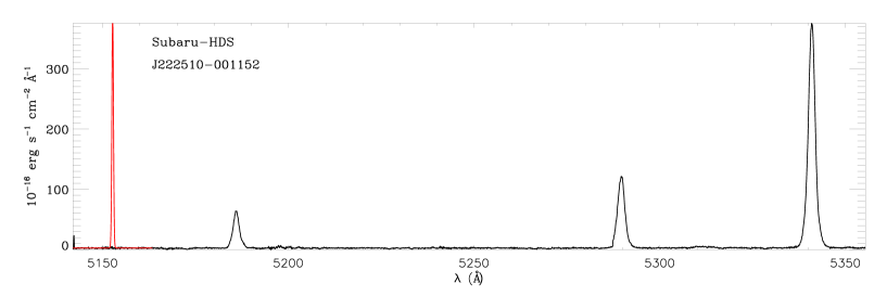
(a)

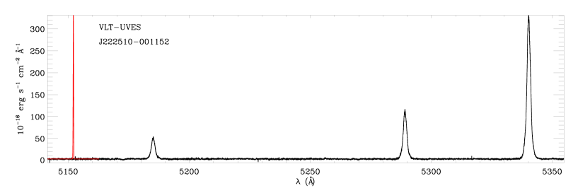
(b)

Figure 5: Examples of the high dispersion spectra obtained for the same object with Subaru HDS (top) and VLT UVES (bottom), showing the region covering $\mathrm{H}\beta\$ and the [OIII] lines at $\lambda\lambda$ 4959,5007 Å. The instrumental profile is shown in red at the left of each spectrum.

57 objects were observed with UVES and 76 with HDS. Five of them were observed with both instruments. During the UVES observing run 16 objects were observed more than once (three times for four objects and four times for another one) in order to estimate better the observational errors, and to link the different nights of the run. Two objects were observed twice with the HDS. The five galaxies observed at both telescopes also served as a link between the observing runs and to compare the performance of both telescopes/instruments and the quality of the nights.

Similarly, 59 sources were observed at OAGH and 59 at OAN, of which 15 were observed at both telescopes.

The UVES data reduction was carried out using the UVES pipeline V4.7.4 under the GASGANO V2.4.0 environment. The reduction entailed the following steps and tasks: (1) master bias generation (uves_cal_mbias), (2) spectral orders reference table generation (uves_cal_predict and uves_cal_orderpos), (3) master flat generation (uves_cal_mflat), (4) wavelength calibration (uves_cal_wavecal), (5) flux calibration (uves_cal_response) and (6) science objects reduction (uves_obs_scired).

The HDS data were reduced using IRAF packages and a script for overscan removal and detector linearity corrections provided by the NAOJ-Subaru telescope team. The reduction procedure entailed the following steps: (1) bias subtraction, (2) generation of spectral order trace template, (3) scattered light removal, (4) flat fielding, (5) 1d spectrum extraction and (6) wavelength calibration.

Typical examples of the high dispersion spectra are shown in Figure 5. The instrumental profile of each setup is also shown on the left.

4 Data analysis.

We have already mentioned in §2 that we observed 128 HIIGx with EW(H$\beta$) $>50$ $\mathrm{\AA}$. From the observed sample we have removed 13 objects which presented problems in the data (low S/N) or showed evidence for a prominent underlying Balmer absorption. We also removed an extra object that presented highly asymmetric emission lines. After this we were left with 114 objects that comprise our ‘initial’ sample (S2).

It was shown by Melnick et al. (1988) that imposing an upper limit to the velocity dispersion such as $\log\sigma($H$\beta)<1.8$ $\mathrm{km\ s^{-1}}$, minimizes the probability of including rotationally supported systems and/or objects with multiple young ionising clusters contributing to the total flux and affecting the line profiles. Therefore from S2 we selected all objects having $\log\sigma($H$\beta)<1.8$ $\mathrm{km\ s^{-1}}$ thus creating sample S3 – our ‘benchmark’ sample – composed of 107 objects.

A summary of the characteristics of the subsamples used in this paper can be found in Table 2 and is further discussed in section 6. Column (1) of Table 2 gives the reference name of the sample, column (2) lists its descriptive name, column (3) gives the constraints that led to the creation of the subsample and column (4) gives the number of objects left in it.

Table 2: Samples Description.

(1)	(2)	(3)	(4)
Sample	Description	Constraints	N
S1	Observed	None	128
S2	Initial	S1 excluding all dubious data eliminated	114
S3	Benchmark	S2 excluding $\log\sigma$ (H$\beta)>1.8$	107
S4	10% cut	S3 excluding $\delta_{flux}(\mathrm{H}\beta)>10$, $\delta_{FWHM}(\mathrm{H}\beta)>10$	93
S5	Restricted	S3 excluding kinematical analysis	69

4.1 Emission line fluxes.

Given the importance of accurate measurements for our results, we will describe in detail our methods.

Total flux and equivalent width of the strongest emission lines were measured from our low dispersion wide-slit spectra. Three methods were used, we have obtained the total flux and equivalent width from single gaussian fits to the line profiles using both the IDL routine gaussfit and the IRAF task splot, and we also measured the fluxes integrated under the line, in order to have a measurement independent of the line shape.

Figure 6 shows a gaussian fit and the corresponding integrated flux measurement for an $\mathrm{H}\beta$ line from our low dispersion data. It is clear from the figure that in the cases when the line is asymmetric, the gaussian fit would not provide a good estimate of the actual flux. In the example shown the difference between the gaussian fit and the integration is $\sim 5.7\%$ in flux.

Table LABEL:tab:tab03 shows the results of our wide-slit low resolution spectroscopy measurements. The data listed have not been corrected for internal extinction. Column (1) is our index number, column (2) is the SDSS name, column (3) is the integrated $\mathrm{H}\beta$ flux measured by us from the SDSS published spectra, columns (4) and (5) are the $\mathrm{H}\beta$ line fluxes as measured from a gaussian fit to the emission line and integrating the line respectively, columns (6) and (7) are the $[\mathrm{O\ III}]\ \lambda\lambda 4959$ and $5007$ line fluxes measured from a gaussian fit, column (8) gives the EW of the $\mathrm{H}\beta$ line as measured from the SDSS spectra and column (9) is a flag that indicates the origin of the data and is described in the table caption.

Figure 7 shows the comparison between SDSS and our low resolution spectra. Clearly most of the objects show an excess flux in our data which could easily be explained as an aperture effect, as the $3\arcsec$ diameter fiber of SDSS in many cases does not cover all the object whereas our spectra were taken with apertures of $8\arcsec-13\arcsec$ in width, hence covering the entire compact object in all cases.

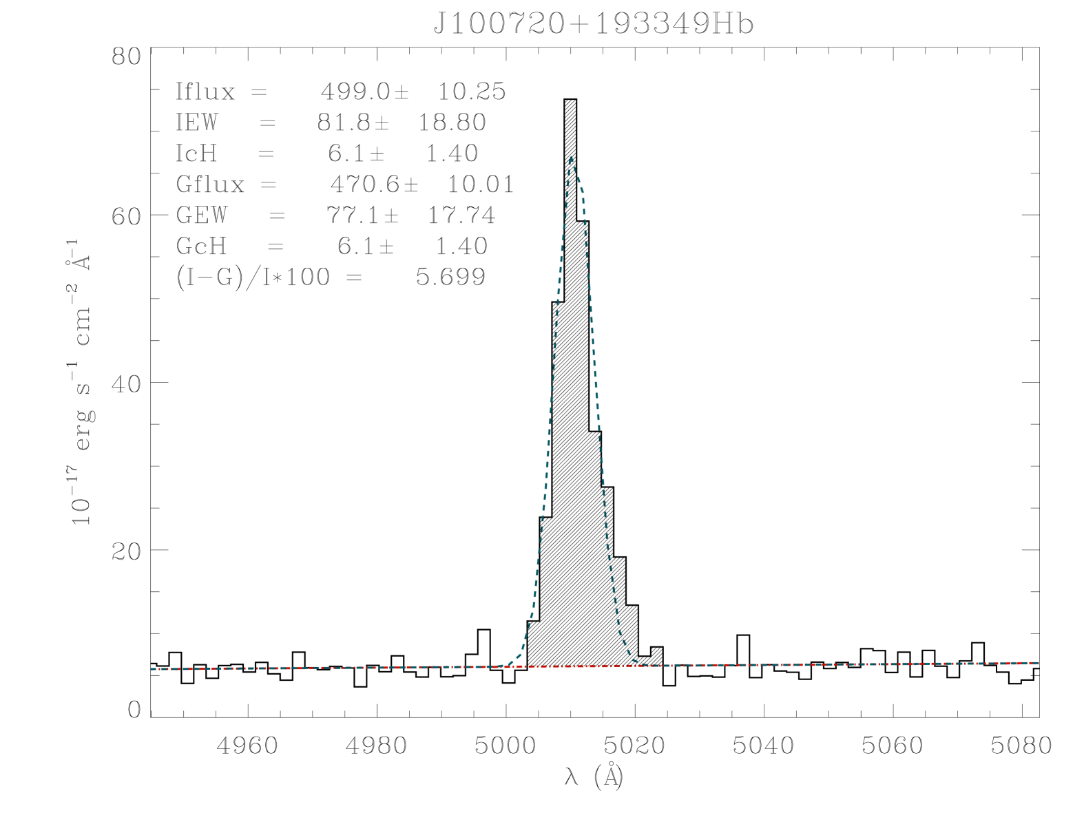
Figure 6: An example of gaussian fit (dashed line) and integration under the line (shaded area) for an $\mathrm{H}\beta$ line from the low dispersion data. The parameters for both fits are shown in the inset.

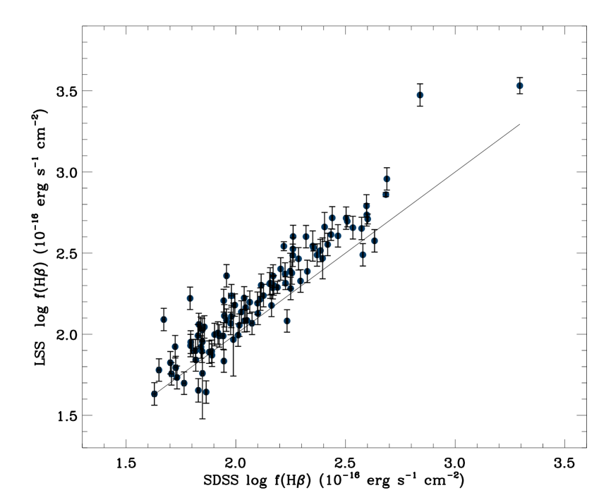
Figure 7: Fluxes measured from SDSS spectra compared with those measured from our low dispersion spectra (LS), the line shows the one-to-one correspondence.

Fluxes and equivalent widths of $[\mathrm{O\ II}]\ \lambda\lambda 3726,3729$, $[\mathrm{O\ III}]\ \lambda\lambda 4363,4959,5007$, $\mathrm{H}\gamma$, $\mathrm{H}\alpha$, $[\mathrm{N\ II}]\ \lambda\lambda 6548,6584$ and $[\mathrm{S\ II}]\ \lambda\lambda 6716,6731$ were also measured from the SDSS spectra when available. We have fitted single gaussians to the line profiles using both the IDL routine gaussfit and the IRAF task splot and, when necessary, we have de-blended lines by multiple gaussian fitting.

Table LABEL:tab:tab04 shows the results for the SDSS spectra line flux measurements as intensity relative to $\mathrm{H}\beta=100$. Columns are: (1) the index number, (2) the SDSS name, (3) and (4) the intensities of $[\mathrm{O\ II}]\ \lambda 3726$ and $\lambda 3729$, (5), (6) and (7) the intensities of $[\mathrm{O\ III}]\ \lambda 4363,\lambda 4959$ and $\lambda 5007$, (8) $\mathrm{H}\gamma$ intensity, (9) $\mathrm{H}\alpha$ intensity, (10) and (11) are the intensities of $[\mathrm{N\ II}]\ \lambda 6548$ and $\lambda 6584$ and (12) and (13) the intensities of the $[\mathrm{S\ II}]\ \lambda 6716$ and $\lambda 6731$ lines. The values given are as measured, not corrected for extinction. The 1$\sigma$ uncertainties for the fluxes are given in percentage.

In all cases, unless otherwise stated in the tables, the uncertainties and equivalent flux of the lines have been estimated from the expressions (Tresse et al., 1999):

$$\sigma_{F} = \sigma_{c}D\sqrt{2N_{pix}+EW/D},$$ (1)

$$\sigma_{EW} = \frac{EW}{F}\sigma_{c}D\sqrt{EW/D+2N_{pix}+(EW/D)^{2}/N_{pix}},$$ (2)

where $\sigma_{c}$ is the mean standard deviation per pixel of the continuum at each side of the line, $D$ is the spectral dispersion in $\mathrm{\AA\ pix^{-1}}$, $N_{pix}$ is the number of pixels covered by the line, $EW$ is the line equivalent width in $\mathrm{\AA}$, $F$ is the flux in units of $\mathrm{erg\ s^{-1}\ cm^{-2}}$. When more than one observation was available, the 1$\sigma$ uncertainty was given as the standard deviation of the individual determinations.

In order to characterise further the sample, a BPT diagram was drawn for the 99 objects of S3 that have a good measurement of $[\mathrm{O\ III}]\lambda$ 5007/ $\mathrm{H}\beta$  and $[\mathrm{N\ II}]\lambda$ 6584/$\mathrm{H}\alpha$  ratios. The diagram is shown in figure 8 where it can be seen that clearly, all objects are located in a narrow strip just below the transition line (Kewley et al., 2001) indicating high excitation and suggesting low metal content and photoionisation by hot main sequence stars, consistent with the expectations for young HII regions.

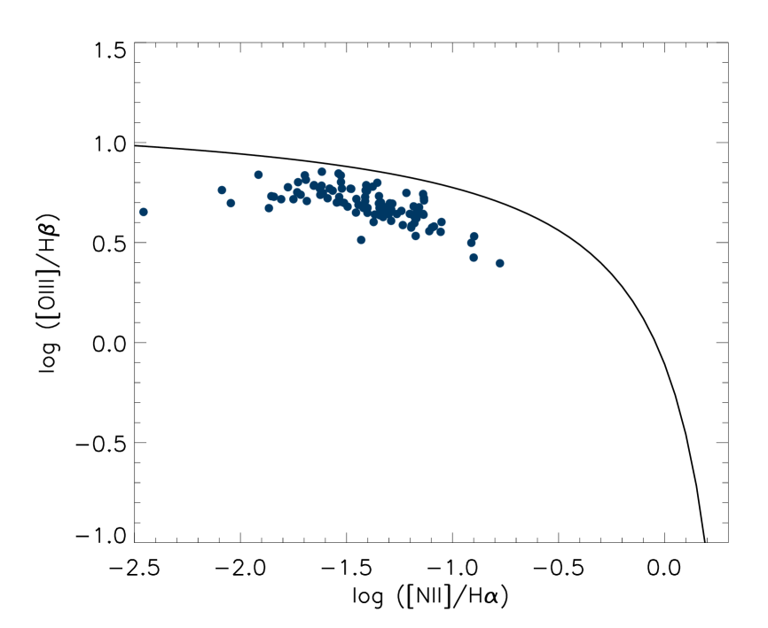
Figure 8: BPT diagram showing the high excitation level of a sample of HIIGx selected mainly as having high equivalent width in their Balmer emission lines. The solid line represents the upper limit for stellar photoionization, from Kewley et al. (2001).The plot shows 99 points from the S3 sample (see text).

4.2 Line profiles

From the two dimensional high dispersion spectra we have obtained the total flux, the position and the full width at half maximum (FWHM) of $\mathrm{H}\beta$ and $[\mathrm{O\ III}]\ \lambda\lambda 4959,5007$Å in each spatial increment i.e. along the slit.

These measurements were used to map the trends in intensity, position, centroid wavelength and FWHM of those emission lines. The intensity or brightness distribution across the object provides information about the sizes of the line and continuum emitting regions. The brightness distribution was used to determine the centroid and FWHM of the line emitting region. On the other hand the trend in the central wavelength of the spectral profile along the spatial direction was used to determine the amount of rotation present.

The trend in FWHM along the slit help us also to verify that there is no FWHM gradient across the object; any important change along the slit could affect the global measurements. In general it was found that the FWHM of the non-rotating systems is almost constant. Those systems with significant gradient or change, were removed from S3 leaving us with the sample used in Chavez et al 2012 paper (S5). We call this procedure the ‘kinematic analysis’ of the emission line profiles and we will discuss in §6 whether this can affect the distance estimator.

The observed spatial FWHM of the emitting region was used to extract the one dimensional spectrum of each object. Three different fits were performed on the 1D spectra profiles (FWHM) of $\mathrm{H}\beta$ and the $[\mathrm{O\ III}]\ \lambda\lambda 4959,5007$Å lines: a single gaussian, two asymmetric gaussians and 3 gaussians (a core plus a blue and a red wing). These fits were performed using the IDL routines gaussfit, arm_asymgaussfit and arm_multgaussfit respectively. Figure 9 shows a typical fit to $\mathrm{H}\beta$; the best fitting to all the sample objects is presented in Appendix A.

Multiple fittings with no initial restrictions are not unique, so we computed using an automatized IDL code, a grid of fits each with slightly different initial conditions. From this set of solutions we chose those that had the minimum $\chi^{2}$. We begin with a blind grid of parameters from which the multiple gaussian fits are constructed, hence some of the resulting fits with small $\chi^{2}$ are not reasonable due to numerical divergence in the fitting procedure. We have eliminated unreasonable results by visual inspection.

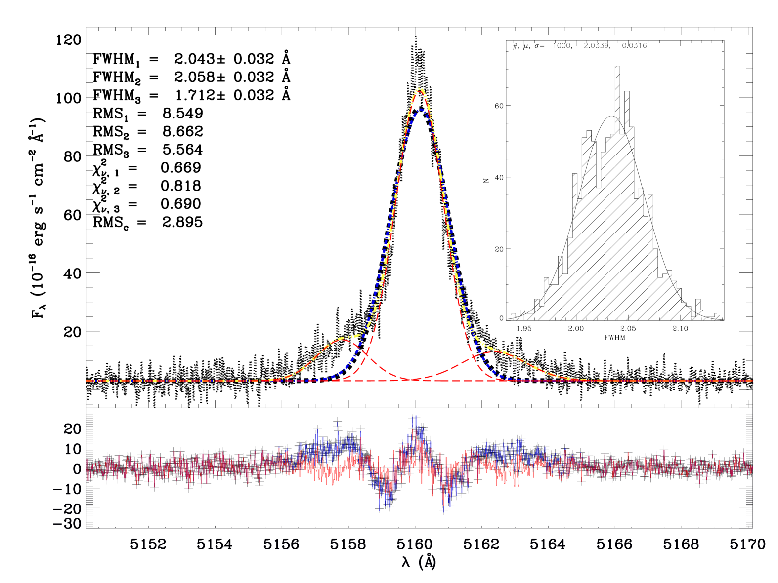
Figure 9: Typical multiple gaussian fit to an $\mathrm{H}\beta$ line. Upper panel: The single gaussian fit is shown with a dashed line (thick black). The asymmetric gaussian fit is indicated by the dash-dotted line (blue). In the three gaussians fit, every gaussian is indicated by long-dashed lines (red) and the total fit by a dash-double-dotted line (yellow). The parameters of the fits are shown in the top left corner. The inset shows the results from the Montecarlo simulation to estimate the errors in the parameters of the best fit. See further details in the text. Lower panel: The residuals from the fits follow the same colour code; the plusses are the residuals from the single gaussian fit whereas the continuous lines are the residuals from the asymmetric and three gaussian fits.

The 1$\sigma$ uncertainties of the FWHM were estimated using a Montecarlo analysis. A set of random realizations of every spectrum was generated using the data poissonian 1$\sigma$ 1-pixel uncertainty. Gaussian fitting for every synthetic spectrum in the set was performed afterwards, and we obtained a distribution of FWHM measurements from which the 1$\sigma$ uncertainty for the FWHM measured in the spectra follows. Average values obtained are 6.3% in H$\beta$ and 3.6% in [OIII].

Table LABEL:tab:tab02 lists the FWHM measurements for the high resolution observations prior to any correction such as instrumental or thermal broadening. Column (1) is the index number, column (2) is the SDSS name, columns (3) and (4) are the right ascension and declination in degrees, column (5) is the heliocentric redshift as taken from the SDSS DR7 spectroscopic data, columns (6) and (7) are the measured $\mathrm{H}\beta$ and $[\mathrm{O\ III}]\ \lambda 5007$ FWHM in Å.

4.3 Emission line widths

The observed velocity dispersions ($\sigma_{o}$) – and their 1$\sigma$ uncertainties – have been derived from the FWHM measurements of the $\mathrm{H}\beta$ and $[\mathrm{O\ III}]\lambda 5007$ lines on the high resolution spectra as:

$$\sigma_{o}\equiv\frac{FWHM}{2\sqrt{2\ ln(2)}}$$ (3)

Corrections for thermal ($\sigma_{th}$), instrumental ($\sigma_{i}$) and fine structure ($\sigma_{fs}$) broadening have been applied. The corrected value is given by the expression:

$$\sigma=\sqrt{\sigma_{o}^{2}-\sigma_{th}^{2}-\sigma_{i}^{2}-\sigma_{fs}^{2}}$$ (4)

We have adopted the value of $\sigma_{fs}(\mathrm{H}\beta)=2.4\ \mathrm{km\ s^{-1}}$ as published in García-Díaz et al. (2008). The 1$\sigma$ uncertainties for the velocity dispersion have been propagated from the $\sigma_{o}$ values.

The high resolution spectra were obtained with two different slit widths. The slit size was initially defined as to cover part of the Petrosian diameter of the objects. For UVES data, for which the slit width was 2^′′ and the slit was uniformly illuminated, $\sigma_{i}$ was directly estimated from sky lines, as usual. The Subaru observations have shown that the 4^′′ slit size used, combined with the excellent seeing during our observations has the unwanted consequence that the slit was not uniformly illuminated for the most compact HIIGx that tend to be also the most distant ones. Thus we have devised a simple procedure to calculate the instrumental broadening correction for the Subaru data. In this case, $\sigma_{i}$ was estimated from the target size; we positioned a rectangular area representing the slit over the corresponding SDSS r band image and measured from the image the FWHM of the object along the dispersion direction. In Figure 10 we plot $\sigma$ (after applying the broadening corrections as described above) for the five objects that have been observed with both instruments. It is clear that the results using both methods are consistent.

Figure 10: Comparison of $\sigma$ values after applying broadening corrections, as described in the text, for the 5 objects observed with both telescopes. The labels are the object indices as in the tables.

The thermal broadening was calculated assuming a Maxwellian velocity distribution of the hydrogen and oxygen ions, from the expression:

$$\sigma_{th}\equiv\sqrt{\frac{kT_{e}}{m}},$$ (5)

where $k$ is the Boltzmann constant, $m$ is the mass of the ion in question and $T_{e}$ is the electron temperature in degrees Kelvin as discussed in §6.4. For the H lines, an object with the sample median $\sigma_{0}$=37km/s, thermal broadening represents about 10%, $\sigma_{fs}$=0.3% and $\sigma_{inst-UVES}$=2% while $\sigma_{inst-HDS}$=9%. For the [OIII] lines, thermal broadening is less than 1%, typically 0.3%.

The obtained velocity dispersions for the $\mathrm{H}\beta$ and $[\mathrm{O\ III}]\lambda 5007$ lines are shown in Table LABEL:tab:tab05, in columns (7) and (8) respectively. Figure 11 shows the distribution of the $\mathrm{H}\beta$ velocity dispersions for the S3 sample (see Table 2).

Figure 11: Distribution of the $\mathrm{H}\beta$ velocity dispersion for the sample S3. The dashed line shows the median of the distribution.

4.4 Extinction and underlying absorption

Reddening correction was performed using the coefficients derived from the Balmer decrement, with $\rm{H}\alpha$, $\rm{H}\beta$ and $\rm{H}\gamma$ fluxes obtained from the SDSS DR7 spectra. However, contamination by the underlying stellar population produces Balmer stellar absorption lines under the Balmer nebular emission lines. This fact alters the observed emission line ratios in such a way that the Balmer decrement and the internal extinction are overestimated (see e.g. Olofsson, 1995).

To correct the extinction determinations for underlying absorption, we use the technique proposed by Rosa-González et al. (2002). The first step is to determine the underlying Balmer absorption ($Q$) and the “true” visual extinction ($A_{V}$) from the observed one ($A_{V}^{*}$).

The ratio between a specific line intensity, $F(\lambda)$, and that of $\mathrm{H}\beta$, $F(\mathrm{H}\beta)$, is given by

$$\frac{F(\lambda)}{F(\mathrm{H}\beta)}=\frac{F_{0}(\lambda)}{F_{0}(\mathrm{H}\beta)}10^{-0.4A_{V}[k(\lambda)-k(\mathrm{H}\beta)]/R_{V}},$$ (6)

where $k(\lambda)=A(\lambda)/E(B-V)$ is given by the adopted extinction law, $R_{V}=A_{V}/E(B-V)$ is the optical total-to-selective extinction ratio and the subscript $0$ indicates unreddened intrinsic values.

We used as reference the theoretical ratios for Case B recombination $F_{0}(\mathrm{H}\alpha)/F_{0}(\mathrm{H}\beta)=2.86$ and $F_{0}(\mathrm{H}\gamma)/F_{0}(\mathrm{H}\beta)=0.47$(Osterbrock, 1989). In the absence of underlying absorption, the observed flux ratios can be expressed as a function of the theoretical ratios and the visual extinction:

$$\log\frac{F(\mathrm{H}\alpha)}{F(\mathrm{H}\beta)} =\log 2.86-0.4[k(\mathrm{H}\alpha)-k(\mathrm{H}\beta)]A_{V}/R_{V}\;,$$ (7)

$$\log\frac{F(\mathrm{H}\gamma)}{F(\mathrm{H}\beta)} =\log 0.47-0.4[k(\mathrm{H}\gamma)-k(\mathrm{H}\beta)]A_{V}/R_{V}\;.$$ (8)

Including the underlying absorption and assuming that the absorption and emission lines have the same widths (González-Delgado et al., 1999), the observed ratio between $\mathrm{H}\alpha$ and $\mathrm{H}\beta$ is given by

$$\frac{F(\mathrm{H}\alpha)}{F(\mathrm{H}\beta)}=\frac{2.86\{1-PQ[W_{+}(\mathrm{H}\beta)/W_{+}(\mathrm{H}\alpha)]\}}{1-Q},$$ (9)

where $W_{+}(\mathrm{H}\alpha)$ and $W_{+}(\mathrm{H}\beta)$ are the equivalent widths in emission for the lines, $Q=W_{-}(\mathrm{H}\beta)/W_{+}(\mathrm{H}\beta)$ is the ratio between the equivalent widths of $\mathrm{H}\beta$ in absorption and in emission and $P=W_{-}(\mathrm{H}\alpha)/W_{-}(\mathrm{H}\beta)$ is the ratio between $\mathrm{H}\alpha$ and $\mathrm{H}\beta$ equivalent widths in absorption.

The value $P$ can be obtained theoretically from spectral evolution models. Olofsson (1995) has shown that for solar abundance and stellar mass in the range $0.1\ \mathrm{M_{\odot}}\leq M\leq 100\ \mathrm{M_{\odot}}$ using a Salpeter IMF, the value of $P$ is close to $1$ with a dispersion $\sim 0.3$ for ages between $1-15\ \mathrm{Myr}$. Since the variation of $P$ produces a change in the $F(\mathrm{H}\alpha)/F(\mathrm{H}\beta)$ ratio of less than 2 % that, given the low extinction in HIIGx, translates in a flux uncertainty well below 1 %, we have assumed $P=1$.

The ratio between $\mathrm{H}\gamma$ and $\mathrm{H}\beta$ is

$$\frac{F(\mathrm{H}\gamma)}{F(\mathrm{H}\beta)}=\frac{0.47-GQ}{1-Q},$$ (10)

where $G=W_{-}(\mathrm{H}\gamma)/W_{-}(\mathrm{H}\beta)$ is the ratio between the equivalent widths in absorption of $\mathrm{H}\gamma$ and $\mathrm{H}\beta$. Olofsson (1995, ; Tables 3a,b ) and González-Delgado et al. (1999, ; Table 1) suggest that the value of the parameter $G$ can also be taken as $1$.

When the theoretical values for the ratios $\log[F(\mathrm{H}\alpha)/F(\mathrm{H}\beta)]=0.46$ and $\log[F(\mathrm{H}\gamma)/F(\mathrm{H}\beta)]=-0.33$, are chosen as the origin, the observed ratios can define a vector for the observed visual extinction ($\mathbf{A_{V}^{*}}$). From equations (7) and (8) and a set of values for $A_{V}$, we define a vector for the “true” visual extinction, whereas from equations (9) and (10) and a set of values of $Q$, we define a vector for the underlying absorption $\mathbf{Q}$. Assuming that the vector relation $\mathbf{Q}+\mathbf{A_{V}}=\mathbf{A_{V}^{*}}$ is satisfied, by minimizing the distance between the position of the vector $\mathbf{A_{V}^{*}}$ and the sum $\mathbf{Q}+\mathbf{A_{V}}$ for every pair of parameters $(Q,A_{V})$, we obtain simultaneously the values for $Q$ and $A_{V}$ that correspond to the observed visual extinction.

The de-reddened fluxes were obtained from the expression

$$F_{o}(\lambda)=F_{obs}(\lambda)10^{0.4A_{V}k(\lambda)/R_{V}},$$ (11)

where the extinction law was taken from Calzetti et al. (2000). The 1$\sigma$ uncertainties were propagated by means of a Monte Carlo procedure.

Finally, the de-reddened fluxes were corrected for underlying absorption. For $\mathrm{H}\beta$ the correction is given by:

$$F(H\beta)=\frac{F_{o}(H\beta)}{1-Q}$$ (12)

The 1$\sigma$ uncertainties were propagated straightforwardly. The results are shown in Table LABEL:tab:tab05, columns (4), (5) and (6) where we give the values for $A_{v}$, $Q$ and $C_{\mathrm{H}\beta}$ respectively.

Table 3: Low resolution and SDSS DR7 $\mathrm{H}\beta$ and $[\mathrm{O\ III}]\ \lambda\lambda 4959,5007$ fluxes and EW($\mathrm{H}\beta$).

(1)	(2)	(3)	(4)	(5)	(6)	(7)	(8)	(9)
Index	Name	F∗($\mathbf{\mathrm{H}\beta}$)	F($\mathbf{\mathrm{H}\beta}$)	F($\mathbf{\mathrm{H}\beta}$)	F($\mathbf{[\mathrm{O\ III}]\ \lambda 4959}$)	F($\mathbf{[\mathrm{O\ III}]\ \lambda 5007}$)	EW($\mathbf{\mathrm{H}\beta}$)	Inst.†
		SDSS DR7	LS Gaussian Fit	LS Integral	LS Gaussian Fit	LS Gaussian Fit	Å
001	J000657+005125	88.1 $\pm$ 1.1	112.7 $\pm$ 11.6	113.0 $\pm$ 11.3	126.9 $\pm$ 8.1	381.7 $\pm$ 22.6	102.2 $\pm$ 5.3	1
002	J001647-104742	167.7 $\pm$ 1.1	231.5 $\pm$ 28.2	236.1 $\pm$ 28.9	298.1 $\pm$ 19.1	882.5 $\pm$ 52.2	67.6 $\pm$ 1.5	1
003	J002339-094848	125.6 $\pm$ 0.9	153.6 $\pm$ 18.7	155.1 $\pm$ 19.0	315.3 $\pm$ 20.2	955.5 $\pm$ 56.5	123.9 $\pm$ 4.1	1
004	J002425+140410	272.0 $\pm$ 1.7	407.3 $\pm$ 43.2	408.1 $\pm$ 41.3	603.2 $\pm$ 48.0	1804.8 $\pm$ 147.0	66.3 $\pm$ 1.3	1
005	J003218+150014	254.3 $\pm$ 1.4	457.0 $\pm$ 91.9	456.0 $\pm$ 96.2	671.9 $\pm$ 43.1	2060.0 $\pm$ 121.8	82.8 $\pm$ 1.7	1
006	J005147+000940	94.8 $\pm$ 0.5	117.3 $\pm$ 14.4	116.6 $\pm$ 14.3	192.1 $\pm$ 12.3	581.1 $\pm$ 34.4	107.8 $\pm$ 2.7	1
007	J005602-101009	65.7 $\pm$ 0.8	66.7 $\pm$ 8.2	66.6 $\pm$ 8.2	88.8 $\pm$ 5.7	252.0 $\pm$ 14.9	52.8 $\pm$ 1.7	1
008	J013258-085337	77.9 $\pm$ 0.7	71.5 $\pm$ 8.8	73.5 $\pm$ 9.1	113.5 $\pm$ 7.3	307.1 $\pm$ 18.2	72.4 $\pm$ 2.3	1
009	J013344+005711	70.5 $\pm$ 1.0	81.4 $\pm$ 10.0	83.8 $\pm$ 10.3	64.7 $\pm$ 4.1	166.6 $\pm$ 9.9	72.3 $\pm$ 3.6	1
010	J014137-091435	90.7 $\pm$ 1.1	116.3 $\pm$ 12.0	116.7 $\pm$ 11.7	—	—	69.8 $\pm$ 3.2	2
011	J014707+135629	115.8 $\pm$ 0.6	154.6 $\pm$ 18.9	156.2 $\pm$ 19.1	288.3 $\pm$ 18.5	867.7 $\pm$ 51.3	163.4 $\pm$ 6.2	1
012	J021852-091218	70.5 $\pm$ 1.1	90.6 $\pm$ 11.1	90.0 $\pm$ 11.0	204.2 $\pm$ 13.1	603.9 $\pm$ 35.7	163.7 $\pm$ 14.4	1
013	J022037-092907	88.0 $\pm$ 0.9	160.3 $\pm$ 19.9	157.6 $\pm$ 19.6	293.8 $\pm$ 18.8	879.0 $\pm$ 52.0	155.4 $\pm$ 7.5	1
014	J024052-082827	177.8 $\pm$ 1.7	187.5 $\pm$ 22.9	191.2 $\pm$ 23.4	474.3 $\pm$ 30.4	1397.0 $\pm$ 82.6	448.6 $\pm$ 45.5	1
015	J024453-082137	69.3 $\pm$ 0.8	107.7 $\pm$ 13.3	108.0 $\pm$ 13.4	149.7 $\pm$ 9.6	440.0 $\pm$ 26.0	99.4 $\pm$ 4.3	1
016	J025426-004122	130.5 $\pm$ 1.0	202.6 $\pm$ 24.7	199.8 $\pm$ 24.5	305.1 $\pm$ 19.6	898.9 $\pm$ 53.2	64.1 $\pm$ 1.8	1
017	J030321-075923	67.5 $\pm$ 0.8	84.3 $\pm$ 8.5	84.4 $\pm$ 8.3	80.4 $\pm$ 5.1	248.3 $\pm$ 14.7	163.4 $\pm$ 30.4	1
018	J031023-083432	59.7 $\pm$ 0.7	73.8 $\pm$ 7.3	73.9 $\pm$ 7.1	—	—	85.3 $\pm$ 3.8	2
019	J033526-003811	67.8 $\pm$ 0.8	104.8 $\pm$ 12.9	105.2 $\pm$ 12.9	188.9 $\pm$ 12.1	541.6 $\pm$ 32.0	111.0 $\pm$ 6.5	1
020	J040937-051805	61.9 $\pm$ 0.6	76.8 $\pm$ 7.6	76.9 $\pm$ 7.4	—	—	131.2 $\pm$ 5.8	2
021	J051519-391741	173.8 $\pm$ 5.2	173.8 $\pm$ 5.2	173.8 $\pm$ 5.2	—	—	187.0 $\pm$ 18.7	3
022	J064650-374322	182.0 $\pm$ 5.5	182.0 $\pm$ 5.5	182.0 $\pm$ 5.5	—	—	50.0 $\pm$ 5.0	3
023	J074806+193146	87.8 $\pm$ 1.1	107.4 $\pm$ 4.3	108.5 $\pm$ 4.9	96.1 $\pm$ 6.2	289.0 $\pm$ 17.1	148.4 $\pm$ 9.5	1
024	J074947+154013	44.6 $\pm$ 0.7	60.6 $\pm$ 7.4	60.6 $\pm$ 7.4	94.2 $\pm$ 6.0	282.5 $\pm$ 16.7	65.4 $\pm$ 3.4	1
025	J080000+274642	97.5 $\pm$ 0.8	125.6 $\pm$ 15.3	125.6 $\pm$ 15.4	116.4 $\pm$ 7.5	315.9 $\pm$ 18.7	55.4 $\pm$ 1.3	1
026	J080619+194927	292.1 $\pm$ 1.2	386.3 $\pm$ 47.1	404.8 $\pm$ 49.4	526.2 $\pm$ 33.7	1610.0 $\pm$ 95.2	79.6 $\pm$ 1.1	1
027	J081334+313252	224.4 $\pm$ 1.0	352.0 $\pm$ 85.8	349.4 $\pm$ 76.1	791.2 $\pm$ 50.7	2348.5 $\pm$ 138.9	89.6 $\pm$ 2.0	1
028	J081403+235328	118.5 $\pm$ 1.9	116.8 $\pm$ 14.3	115.7 $\pm$ 14.3	205.4 $\pm$ 13.2	599.3 $\pm$ 35.4	109.7 $\pm$ 7.3	1
029	J081420+575008	71.9 $\pm$ 0.6	109.0 $\pm$ 13.3	108.8 $\pm$ 13.3	155.6 $\pm$ 10.0	459.7 $\pm$ 27.2	58.0 $\pm$ 1.6	1
030	J081737+520236	248.7 $\pm$ 1.5	284.9 $\pm$ 72.0	292.5 $\pm$ 82.8	456.4 $\pm$ 29.2	1303.0 $\pm$ 77.0	61.4 $\pm$ 1.2	1
031	J082520+082723	42.6 $\pm$ 0.7	43.2 $\pm$ 5.3	43.1 $\pm$ 5.3	105.5 $\pm$ 6.8	292.5 $\pm$ 17.3	61.1 $\pm$ 3.3	1
032	J082530+504804	106.0 $\pm$ 0.9	128.4 $\pm$ 15.7	128.0 $\pm$ 15.7	229.3 $\pm$ 14.7	654.2 $\pm$ 38.7	119.6 $\pm$ 4.1	1
033	J082722+202612	88.6 $\pm$ 1.2	126.9 $\pm$ 15.5	128.4 $\pm$ 15.7	208.6 $\pm$ 13.4	628.8 $\pm$ 37.2	77.5 $\pm$ 3.4	1
034	J083946+140033	69.4 $\pm$ 0.7	82.5 $\pm$ 10.1	83.3 $\pm$ 10.2	106.9 $\pm$ 6.9	309.4 $\pm$ 18.3	84.2 $\pm$ 2.9	1
035	J084000+180531	112.7 $\pm$ 0.9	123.5 $\pm$ 15.1	122.4 $\pm$ 15.0	252.1 $\pm$ 16.2	733.4 $\pm$ 43.4	183.9 $\pm$ 10.0	1
036	J084029+470710	262.4 $\pm$ 1.8	350.5 $\pm$ 42.7	356.9 $\pm$ 43.5	651.1 $\pm$ 41.7	1952.0 $\pm$ 115.4	215.6 $\pm$ 10.7	1
037	J084056+022030	73.2 $\pm$ 0.7	92.1 $\pm$ 9.3	92.3 $\pm$ 9.1	36.6 $\pm$ 2.3	107.7 $\pm$ 6.4	71.2 $\pm$ 2.3	1
038	J084219+300703	95.4 $\pm$ 0.7	126.6 $\pm$ 15.4	128.8 $\pm$ 15.7	175.0 $\pm$ 11.2	507.4 $\pm$ 30.0	55.8 $\pm$ 1.1	1
039	J084220+115000	223.8 $\pm$ 1.4	309.9 $\pm$ 34.9	312.4 $\pm$ 34.0	—	—	126.1 $\pm$ 4.2	2
040	J084414+022621	168.9 $\pm$ 0.8	201.9 $\pm$ 17.0	205.0 $\pm$ 20.1	393.1 $\pm$ 25.2	1165.0 $\pm$ 68.9	111.4 $\pm$ 2.2	1
041	J084527+530852	197.4 $\pm$ 1.1	207.8 $\pm$ 25.6	213.2 $\pm$ 26.4	382.0 $\pm$ 24.5	1096.0 $\pm$ 64.8	149.7 $\pm$ 5.5	1
042	J084634+362620	320.0 $\pm$ 1.6	457.1 $\pm$ 53.2	461.5 $\pm$ 52.0	—	—	78.8 $\pm$ 1.5	2
043	J085221+121651	374.9 $\pm$ 1.4	438.0 $\pm$ 53.4	440.6 $\pm$ 53.8	868.6 $\pm$ 55.7	2594.0 $\pm$ 153.4	168.2 $\pm$ 3.7	1
044	J090418+260106	111.8 $\pm$ 1.0	145.9 $\pm$ 15.4	146.5 $\pm$ 15.0	—	—	64.1 $\pm$ 1.7	2
045	J090506+223833	80.6 $\pm$ 0.6	98.2 $\pm$ 12.1	99.5 $\pm$ 12.3	—	—	123.8 $\pm$ 4.1	2
046	J090531+033530	109.1 $\pm$ 0.8	166.3 $\pm$ 20.5	165.9 $\pm$ 20.5	273.3 $\pm$ 17.5	879.2 $\pm$ 52.0	125.8 $\pm$ 4.0	1
047	J091434+470207	399.5 $\pm$ 1.5	505.5 $\pm$ 38.6	510.6 $\pm$ 38.5	927.4 $\pm$ 52.6	2702.5 $\pm$ 134.9	112.1 $\pm$ 2.3	1
048	J091640+182807	110.8 $\pm$ 0.8	145.8 $\pm$ 17.8	145.0 $\pm$ 17.7	—	—	131.3 $\pm$ 5.3	2
049	J091652+003113	65.5 $\pm$ 0.8	79.8 $\pm$ 9.7	79.3 $\pm$ 9.7	112.4 $\pm$ 7.2	339.6 $\pm$ 20.1	81.6 $\pm$ 3.7	1
050	J092540+063116	67.1 $\pm$ 0.7	98.3 $\pm$ 12.0	98.3 $\pm$ 12.0	147.1 $\pm$ 9.4	437.5 $\pm$ 25.9	90.5 $\pm$ 3.6	1
051	J092749+084037	83.9 $\pm$ 1.0	94.6 $\pm$ 11.6	93.3 $\pm$ 11.4	84.0 $\pm$ 5.4	268.1 $\pm$ 15.9	100.7 $\pm$ 5.6	1
052	J092918+002813	70.4 $\pm$ 0.9	101.0 $\pm$ 12.5	91.6 $\pm$ 11.4	185.5 $\pm$ 11.9	530.8 $\pm$ 31.4	182.8 $\pm$ 15.5	1
053	J093006+602653	318.4 $\pm$ 1.4	454.7 $\pm$ 52.9	459.1 $\pm$ 51.7	878.0 $\pm$ 56.3	2540.0 $\pm$ 150.2	123.4 $\pm$ 3.5	1
054	J093424+222522	99.3 $\pm$ 1.1	128.3 $\pm$ 13.4	128.8 $\pm$ 13.0	—	—	108.1 $\pm$ 4.4	2
055	J093813+542825	193.2 $\pm$ 1.1	282.5 $\pm$ 34.4	288.1 $\pm$ 35.2	410.9 $\pm$ 26.3	1202.0 $\pm$ 71.1	84.4 $\pm$ 2.0	1
056	J094000+203122	102.6 $\pm$ 0.9	98.7 $\pm$ 12.1	98.5 $\pm$ 12.2	123.9 $\pm$ 7.9	377.2 $\pm$ 22.3	85.8 $\pm$ 2.9	1
057	J094252+354725	193.2 $\pm$ 1.1	264.3 $\pm$ 29.3	266.2 $\pm$ 28.6	—	—	91.6 $\pm$ 2.0	2
058	J094254+340411	64.0 $\pm$ 1.1	81.5 $\pm$ 10.0	78.9 $\pm$ 9.7	142.8 $\pm$ 9.2	414.1 $\pm$ 24.5	188.6 $\pm$ 20.4	1
059	J094809+425713	158.5 $\pm$ 1.2	213.1 $\pm$ 23.2	214.4 $\pm$ 22.6	—	—	100.1 $\pm$ 3.5	2
060	J095000+300341	147.4 $\pm$ 1.3	196.7 $\pm$ 24.0	194.4 $\pm$ 23.8	304.6 $\pm$ 19.5	933.6 $\pm$ 55.2	94.5 $\pm$ 3.5	1
061	J095023+004229	125.9 $\pm$ 1.1	132.4 $\pm$ 16.2	134.8 $\pm$ 16.5	240.2 $\pm$ 15.4	768.2 $\pm$ 45.4	118.9 $\pm$ 3.7	1
062	J095131+525936	181.9 $\pm$ 1.7	299.2 $\pm$ 36.5	303.0 $\pm$ 37.0	605.7 $\pm$ 38.8	1792.0 $\pm$ 106.0	180.8 $\pm$ 8.0	1
063	J095226+021759	103.0 $\pm$ 1.0	133.5 $\pm$ 14.0	134.0 $\pm$ 13.6	—	—	111.2 $\pm$ 4.2	2
064	J095227+322809	147.9 $\pm$ 1.0	226.1 $\pm$ 27.8	225.2 $\pm$ 27.8	449.1 $\pm$ 28.8	1304.0 $\pm$ 77.1	92.5 $\pm$ 2.8	1
065	J095545+413429	191.3 $\pm$ 1.5	261.4 $\pm$ 29.0	263.2 $\pm$ 28.3	—	—	67.9 $\pm$ 1.8	2
066	J100720+193349	58.1 $\pm$ 0.9	47.2 $\pm$ 5.8	50.0 $\pm$ 6.2	82.6 $\pm$ 5.3	246.9 $\pm$ 14.6	137.5 $\pm$ 11.5	1
067	J100746+025228	180.2 $\pm$ 0.8	237.8 $\pm$ 29.1	238.5 $\pm$ 29.3	395.5 $\pm$ 25.3	1137.0 $\pm$ 67.2	129.4 $\pm$ 3.7	1
068	J101036+641242	234.3 $\pm$ 1.1	312.9 $\pm$ 38.1	307.5 $\pm$ 37.5	414.6 $\pm$ 26.6	1220.0 $\pm$ 72.1	76.1 $\pm$ 1.1	1
069	J101042+125516	341.8 $\pm$ 1.3	452.3 $\pm$ 56.2	448.7 $\pm$ 55.9	813.6 $\pm$ 52.1	2409.0 $\pm$ 142.4	92.2 $\pm$ 1.2	1
070	J101136+263027	90.6 $\pm$ 0.7	122.8 $\pm$ 15.0	121.5 $\pm$ 14.9	181.0 $\pm$ 11.6	552.2 $\pm$ 32.7	91.0 $\pm$ 2.9	1
071	J101157+130822	88.2 $\pm$ 1.3	112.8 $\pm$ 11.7	113.2 $\pm$ 11.4	—	—	351.2 $\pm$ 35.2	2
072	J101430+004755	73.4 $\pm$ 0.9	92.3 $\pm$ 9.4	92.6 $\pm$ 9.1	—	—	81.1 $\pm$ 3.4	2
073	J101458+193219	58.4 $\pm$ 0.8	72.1 $\pm$ 7.2	72.2 $\pm$ 7.0	—	—	104.9 $\pm$ 7.0	2
074	J102429+052451	275.1 $\pm$ 1.4	519.5 $\pm$ 63.5	524.7 $\pm$ 64.3	889.4 $\pm$ 57.0	2553.0 $\pm$ 151.0	100.8 $\pm$ 2.1	1
075	J102732-284201	158.5 $\pm$ 3.2	158.5 $\pm$ 3.2	158.5 $\pm$ 3.2	—	—	73.0 $\pm$ 7.3	3
076	J103226+271755	53.9 $\pm$ 0.7	53.2 $\pm$ 6.7	53.7 $\pm$ 6.8	100.7 $\pm$ 6.5	308.6 $\pm$ 18.2	192.4 $\pm$ 13.5	1
077	J103328+070801	395.6 $\pm$ 1.6	545.1 $\pm$ 66.4	530.7 $\pm$ 64.8	493.6 $\pm$ 31.6	1435.0 $\pm$ 84.8	52.3 $\pm$ 0.5	1
078	J103412+014249	47.1 $\pm$ 0.7	57.0 $\pm$ 5.6	57.0 $\pm$ 5.4	—	—	93.4 $\pm$ 5.6	2
079	J103509+094516	77.6 $\pm$ 0.8	78.9 $\pm$ 9.7	77.4 $\pm$ 9.5	130.3 $\pm$ 8.3	379.7 $\pm$ 22.5	70.9 $\pm$ 2.7	1
080	J103726+270759	62.1 $\pm$ 0.8	77.1 $\pm$ 7.7	77.2 $\pm$ 7.5	—	—	67.4 $\pm$ 2.6	2
081	J104457+035313	429.5 $\pm$ 1.9	373.1 $\pm$ 45.7	375.8 $\pm$ 46.1	688.7 $\pm$ 44.1	2038.0 $\pm$ 120.5	332.5 $\pm$ 18.1	1
082	J104554+010405	394.6 $\pm$ 1.4	593.3 $\pm$ 72.2	610.9 $\pm$ 74.6	982.0 $\pm$ 62.9	2736.0 $\pm$ 161.8	170.7 $\pm$ 4.8	1
083	J104653+134645	182.7 $\pm$ 0.9	402.3 $\pm$ 49.1	396.5 $\pm$ 48.5	712.4 $\pm$ 45.7	2092.0 $\pm$ 123.7	210.0 $\pm$ 9.0	1
084	J104723+302144	487.4 $\pm$ 2.4	901.0 $\pm$ 109.6	916.4 $\pm$ 111.8	1319.0 $\pm$ 84.5	3892.0 $\pm$ 230.1	65.7 $\pm$ 1.0	1
085	J104755+073951	80.9 $\pm$ 1.5	102.6 $\pm$ 10.6	102.9 $\pm$ 10.3	—	—	181.6 $\pm$ 15.8	2
086	J104829+111520	70.1 $\pm$ 0.9	76.8 $\pm$ 9.6	75.4 $\pm$ 9.4	148.5 $\pm$ 9.5	406.9 $\pm$ 24.1	108.8 $\pm$ 6.1	1
087	J105032+153806	243.0 $\pm$ 1.1	315.7 $\pm$ 38.6	325.4 $\pm$ 39.8	688.3 $\pm$ 44.1	1980.0 $\pm$ 117.1	206.7 $\pm$ 8.0	1
088	J105040+342947	143.0 $\pm$ 1.0	198.9 $\pm$ 24.3	204.3 $\pm$ 25.0	334.3 $\pm$ 21.4	980.0 $\pm$ 57.9	120.5 $\pm$ 4.0	1
089	J105108+131927	62.3 $\pm$ 0.6	91.2 $\pm$ 11.4	90.9 $\pm$ 11.3	123.5 $\pm$ 7.9	357.5 $\pm$ 21.1	54.1 $\pm$ 1.6	1
090	J105210+032713	40.9 $\pm$ 0.8	49.0 $\pm$ 4.8	49.0 $\pm$ 4.6	—	—	66.1 $\pm$ 3.8	2
091	J105326+043014	109.3 $\pm$ 0.9	119.1 $\pm$ 14.5	120.7 $\pm$ 14.8	—	—	68.7 $\pm$ 2.1	2
092	J105331+011740	75.6 $\pm$ 0.8	77.7 $\pm$ 9.5	78.0 $\pm$ 9.6	—	—	81.7 $\pm$ 3.2	2
093	J105741+653539	160.1 $\pm$ 0.8	252.9 $\pm$ 30.8	252.7 $\pm$ 30.9	—	—	68.4 $\pm$ 1.2	2
094	J105940+080056	133.7 $\pm$ 1.1	170.1 $\pm$ 20.9	171.0 $\pm$ 21.0	275.6 $\pm$ 17.7	789.8 $\pm$ 46.7	74.8 $\pm$ 2.1	1
095	J110838+223809	171.3 $\pm$ 1.5	231.9 $\pm$ 25.4	233.4 $\pm$ 24.8	238.9 $\pm$ 15.3	717.4 $\pm$ 42.4	134.2 $\pm$ 5.3	1
096	J114212+002003	692.0 $\pm$ 3.5	1056.2 $\pm$ 132.4	1070.7 $\pm$ 129.7	2773.0 $\pm$ 177.7	8456.0 $\pm$ 500.0	57.5 $\pm$ 0.8	1
097	J115023-003141	95.5 $\pm$ 2.9	95.5 $\pm$ 2.9	95.5 $\pm$ 2.9	—	—	52.0 $\pm$ 5.2	3
098	J121329+114056	211.8 $\pm$ 1.4	243.5 $\pm$ 29.6	244.3 $\pm$ 29.8	505.3 $\pm$ 32.4	1530.0 $\pm$ 90.5	96.3 $\pm$ 2.7	1
099	J121717-280233	223.9 $\pm$ 4.5	223.9 $\pm$ 4.5	223.9 $\pm$ 4.5	—	—	294.0 $\pm$ 29.4	3
100	J125305-031258	1971.9 $\pm$ 3.5	3405.5 $\pm$ 372.3	3402.6 $\pm$ 390.9	7357.0 $\pm$ 464.6	22180.0 $\pm$ 1038.4	238.9 $\pm$ 7.3	1
101	J130119+123959	225.9 $\pm$ 1.1	337.0 $\pm$ 17.7	342.3 $\pm$ 14.5	364.6 $\pm$ 23.4	1076.0 $\pm$ 63.6	105.9 $\pm$ 1.9	1
102	J131235+125743	143.6 $\pm$ 1.0	208.0 $\pm$ 48.1	203.9 $\pm$ 49.6	343.9 $\pm$ 22.0	1007.9 $\pm$ 59.6	96.7 $\pm$ 2.9	1
103	J132347-013252	154.9 $\pm$ 1.3	194.4 $\pm$ 12.1	193.4 $\pm$ 17.1	471.9 $\pm$ 10.3	1411.5 $\pm$ 45.5	288.7 $\pm$ 20.9	1
104	J132549+330354	379.3 $\pm$ 1.4	309.8 $\pm$ 37.7	307.2 $\pm$ 37.5	605.5 $\pm$ 38.8	1826.0 $\pm$ 108.0	120.0 $\pm$ 3.1	1
105	J133708-325528	257.0 $\pm$ 5.1	257.0 $\pm$ 5.1	257.0 $\pm$ 5.1	—	—	263.0 $\pm$ 26.3	3
106	J134531+044232	165.7 $\pm$ 0.9	348.6 $\pm$ 20.5	347.8 $\pm$ 23.7	575.4 $\pm$ 14.1	1722.7 $\pm$ 54.6	67.9 $\pm$ 1.3	1
107	J142342+225728	177.1 $\pm$ 1.2	245.4 $\pm$ 61.0	241.2 $\pm$ 60.2	436.7 $\pm$ 28.0	1255.0 $\pm$ 74.2	135.9 $\pm$ 4.1	1
108	J144805-011057	482.9 $\pm$ 1.5	715.6 $\pm$ 24.2	725.3 $\pm$ 20.9	1599.6 $\pm$ 76.0	4788.4 $\pm$ 124.0	158.0 $\pm$ 4.5	1
109	J162152+151855	322.0 $\pm$ 1.3	491.6 $\pm$ 45.7	496.6 $\pm$ 41.7	712.7 $\pm$ 45.6	2107.7 $\pm$ 173.5	151.1 $\pm$ 3.9	1
110	J171236+321633	148.8 $\pm$ 0.8	200.1 $\pm$ 33.0	199.5 $\pm$ 28.9	365.7 $\pm$ 54.7	1079.5 $\pm$ 155.2	184.1 $\pm$ 8.1	1
111	J192758-413432	2630.3 $\pm$ 5.3	2630.3 $\pm$ 5.3	2630.3 $\pm$ 5.3	—	—	87.0 $\pm$ 8.7	3
112	J210114-055510	53.3 $\pm$ 0.8	61.0 $\pm$ 7.5	62.1 $\pm$ 7.7	102.9 $\pm$ 6.6	304.1 $\pm$ 18.0	115.4 $\pm$ 7.9	1
113	J210501-062238	46.9 $\pm$ 0.6	56.8 $\pm$ 5.5	56.8 $\pm$ 5.4	40.3 $\pm$ 2.6	119.8 $\pm$ 7.1	69.0 $\pm$ 2.8	1
114	J211527-075951	125.7 $\pm$ 1.0	165.7 $\pm$ 17.6	166.5 $\pm$ 17.2	—	—	143.7 $\pm$ 6.2	2
115	J211902-074226	52.9 $\pm$ 0.6	82.5 $\pm$ 10.1	84.9 $\pm$ 10.4	132.7 $\pm$ 8.5	395.9 $\pm$ 23.4	87.3 $\pm$ 3.8	1
116	J212043+010006	67.9 $\pm$ 0.9	84.9 $\pm$ 8.6	85.1 $\pm$ 8.3	—	—	74.3 $\pm$ 2.8	2
117	J212332-074831	50.4 $\pm$ 0.7	67.2 $\pm$ 8.2	66.8 $\pm$ 8.2	103.7 $\pm$ 6.6	302.4 $\pm$ 17.9	65.1 $\pm$ 3.1	1
118	J214350-072003	47.7 $\pm$ 0.6	57.9 $\pm$ 5.6	57.9 $\pm$ 5.5	—	—	69.1 $\pm$ 2.9	2
119	J220802+131334	62.2 $\pm$ 0.7	84.5 $\pm$ 10.3	85.2 $\pm$ 10.4	138.1 $\pm$ 8.8	377.0 $\pm$ 22.3	79.1 $\pm$ 2.8	1
120	J221823+003918	38.5 $\pm$ 0.6	45.9 $\pm$ 4.4	45.8 $\pm$ 4.3	—	—	66.3 $\pm$ 3.6	2
121	J222510-001152	145.4 $\pm$ 1.0	146.6 $\pm$ 17.9	150.6 $\pm$ 18.4	297.9 $\pm$ 19.1	896.5 $\pm$ 53.0	159.2 $\pm$ 6.8	1
122	J224556+125022	129.3 $\pm$ 0.9	161.0 $\pm$ 19.6	164.5 $\pm$ 20.1	177.5 $\pm$ 11.4	532.9 $\pm$ 31.5	79.7 $\pm$ 1.8	1
123	J225140+132713	209.1 $\pm$ 1.0	401.2 $\pm$ 48.8	398.8 $\pm$ 48.6	548.7 $\pm$ 35.2	1612.0 $\pm$ 95.3	61.8 $\pm$ 0.9	1
124	J230117+135230	99.0 $\pm$ 0.9	150.6 $\pm$ 18.4	150.3 $\pm$ 18.4	209.5 $\pm$ 13.4	644.4 $\pm$ 38.1	104.7 $\pm$ 4.2	1
125	J230123+133314	182.0 $\pm$ 1.3	332.9 $\pm$ 40.6	335.9 $\pm$ 41.0	547.9 $\pm$ 35.1	1662.0 $\pm$ 98.3	147.0 $\pm$ 5.0	1
126	J230703+011311	103.2 $\pm$ 0.8	108.4 $\pm$ 13.3	108.8 $\pm$ 13.4	131.1 $\pm$ 8.4	385.1 $\pm$ 22.8	79.6 $\pm$ 2.1	1
127	J231442+010621	50.9 $\pm$ 1.0	57.4 $\pm$ 7.0	57.3 $\pm$ 7.0	78.2 $\pm$ 5.0	226.0 $\pm$ 13.4	76.1 $\pm$ 5.4	1
128	J232936-011056	82.8 $\pm$ 0.9	100.0 $\pm$ 12.3	103.2 $\pm$ 12.7	210.3 $\pm$ 13.5	591.1 $\pm$ 35.0	91.8 $\pm$ 3.9	1
∗ All the fluxes are given in units of $10^{-16}\ \mathrm{erg\ s^{-1}cm^{-2}}$.
† The instrument flag indicates the origin of the data. $1:$ Directly measured using long slit as described in the text. $2$: from aperture corrected
SDSS DR7 measurements. $3:$ from Terlevich et al. (1991), in this case errors in fluxes and EW are taken directly form the cited source.

Table 4: Line intensity ratios with respect to $\mathrm{H}\beta=100$, 1$\sigma$ uncertainties in % are shown in parenthesis. Our measurements from SDSS DR7.

(1)	(2)	(3)	(4)	(5)	(6)	(7)	(8)	(9)	(10)	(11)	(12)	(13)
Index	Name	$\mathbf{[\mathrm{O\ II}]}$	$\mathbf{[\mathrm{O\ II}]}$	$\mathbf{[\mathrm{O\ III}]}$	$\mathbf{[\mathrm{O\ III}]}$	$\mathbf{[\mathrm{O\ III}]}$	$\mathbf{\mathrm{H}\gamma}$	$\mathbf{\mathrm{H}\alpha}$	$\mathbf{[\mathrm{N\ II}]}$	$\mathbf{[\mathrm{N\ II}]}$	$\mathbf{[\mathrm{S\ II}]}$	$\mathbf{[\mathrm{S\ II}]}$
		$\lambda 3726$	$\lambda 3729$	$\lambda 4363$	$\lambda 4959$	$\lambda 5007$			$\lambda 6548$	$\lambda 6584$	$\lambda 6716$	$\lambda 6731$
001	J000657+005125	81.4 (37.0)	101.8 (32.3)	8.51 (8.9)	194 (1.9)	581 (1.8)	43.9 (3.0)	344 (1.8)	6.07 (14.1)	15.8 (6.6)	20.7 (3.6)	15.9 (4.8)
002	J001647-104742	84.1 (3.1)	119.9 (2.5)	4.70 (10.9)	136 (1.2)	409 (1.1)	40.1 (2.0)	358 (1.1)	5.88 (3.0)	18.0 (1.8)	33.3 (1.4)	24.9 (1.4)
003	J002339-094848	64.9 (3.2)	99.3 (2.4)	7.30 (6.2)	207 (1.0)	616 (0.9)	42.1 (1.8)	377 (0.9)	3.29 (11.6)	9.2 (4.8)	19.8 (1.5)	15.0 (1.8)
004	J002425+140410	—	—	3.08 (12.8)	139 (0.9)	423 (0.7)	42.6 (1.5)	335 (0.8)	5.26 (5.9)	15.6 (2.5)	17.6 (1.4)	13.3 (1.8)
005	J003218+150014	—	—	6.21 (5.9)	163 (0.7)	481 (0.6)	44.7 (1.3)	304 (0.6)	3.49 (5.9)	9.7 (2.6)	17.4 (1.0)	12.5 (1.3)
006	J005147+000940	45.1 (6.6)	62.6 (5.3)	12.37 (3.5)	176 (0.9)	526 (0.7)	47.0 (1.4)	283 (0.8)	1.38 (16.8)	4.1 (7.0)	8.7 (2.8)	6.6 (3.2)
007	J005602-101009	107.3 (4.0)	168.5 (3.2)	5.72 (36.5)	102 (1.8)	317 (1.6)	42.4 (4.3)	335 (1.5)	13.40 (5.5)	41.5 (2.9)	34.3 (2.3)	27.8 (2.5)
008	J013258-085337	137.0 (2.6)	178.0 (2.3)	2.44 (23.4)	116 (1.4)	352 (1.4)	44.2 (2.4)	287 (1.4)	6.14 (6.7)	22.2 (3.4)	36.1 (2.2)	25.6 (3.1)
009	J013344+005711	87.3 (38.2)	75.6 (38.8)	9.06 (9.2)	187 (1.8)	573 (1.6)	45.1 (2.9)	318 (1.5)	2.84 (11.3)	8.4 (4.7)	16.4 (2.5)	11.7 (3.5)
010	J014137-091435	—	—	7.25 (12.1)	182 (1.5)	572 (1.3)	43.0 (3.3)	357 (1.4)	2.85 (12.9)	9.0 (5.3)	22.5 (3.1)	16.6 (3.5)
011	J014707+135629	45.4 (6.4)	61.1 (5.4)	10.70 (3.3)	200 (1.3)	604 (1.3)	44.7 (1.7)	335 (1.5)	4.04 (21.9)	11.3 (9.2)	11.7 (1.6)	10.0 (1.7)
012	J021852-091218	—	—	13.16 (8.8)	234 (2.1)	698 (1.8)	41.8 (4.1)	364 (1.7)	1.87 (17.6)	4.4 (8.0)	11.4 (5.2)	8.3 (7.0)
013	J022037-092907	66.2 (27.2)	85.8 (23.1)	6.81 (13.4)	176 (2.7)	525 (3.1)	44.8 (3.2)	313 (3.0)	8.29 (23.5)	23.6 (11.1)	18.7 (3.3)	15.6 (4.0)
014	J024052-082827	—	—	14.31 (6.4)	242 (5.2)	729 (4.4)	44.5 (4.8)	297 (6.6)	38.12 (17.6)	9.7 (38.7)	4.7 (9.4)	4.3 (9.2)
015	J024453-082137	77.1 (24.8)	109.2 (20.1)	6.60 (9.2)	150 (1.4)	448 (1.3)	44.6 (2.6)	320 (1.3)	4.36 (13.1)	11.4 (5.6)	24.6 (2.3)	17.3 (4.4)
016	J025426-004122	—	—	7.72 (10.6)	149 (1.2)	439 (1.0)	41.2 (2.3)	331 (1.0)	4.40 (5.4)	12.9 (1.9)	23.9 (1.4)	17.4 (1.4)
017	J030321-075923	26.7 (16.5)	55.0 (10.3)	12.04 (6.5)	201 (2.8)	609 (3.9)	42.9 (3.3)	282 (3.8)	25.60 (12.5)	8.2 (28.5)	6.6 (24.7)	7.6 (24.0)
018	J031023-083432	76.7 (17.2)	104.1 (14.2)	4.69 (16.2)	162 (1.7)	465 (1.6)	42.4 (2.9)	306 (1.6)	5.85 (14.2)	15.1 (5.1)	20.0 (2.3)	14.1 (3.1)
019	J033526-003811	40.8 (44.4)	68.8 (32.0)	9.73 (9.1)	174 (1.9)	520 (1.6)	42.5 (3.6)	343 (1.6)	1.68 (16.0)	5.3 (10.5)	14.3 (2.6)	8.9 (3.1)
020	J040937-051805	70.5 (14.4)	74.8 (13.3)	6.97 (6.7)	201 (1.7)	602 (1.6)	44.4 (2.2)	333 (1.5)	3.40 (14.7)	10.1 (6.7)	20.4 (3.3)	15.4 (4.1)
021	J051519-391741	—	—	—	—	—	46.2 (15.3)	357 (10.4)	—	—	—	—
022	J064650-374322	—	—	—	—	—	39.6 (15.3)	428 (10.4)	—	—	—	—
023	J074806+193146	91.2 (3.9)	107.2 (3.6)	2.89 (21.8)	140 (2.0)	419 (1.8)	43.1 (2.9)	371 (2.1)	5.91 (20.4)	19.2 (7.8)	25.5 (2.3)	19.0 (2.3)
024	J074947+154013	77.0 (17.9)	106.4 (14.8)	4.92 (26.0)	165 (2.3)	487 (1.8)	45.5 (4.3)	334 (1.8)	6.44 (12.7)	21.9 (5.0)	22.0 (5.4)	16.5 (8.4)
025	J080000+274642	83.7 (2.9)	115.3 (2.5)	5.72 (14.9)	177 (1.3)	536 (1.2)	41.1 (2.8)	355 (1.3)	4.98 (8.0)	13.7 (3.8)	23.7 (2.3)	17.5 (2.3)
026	J080619+194927	82.1 (2.3)	102.9 (2.0)	3.48 (11.4)	143 (1.0)	442 (1.0)	42.5 (1.4)	334 (1.4)	8.22 (14.3)	22.5 (6.0)	24.3 (1.2)	18.7 (1.4)
027	J081334+313252	—	—	9.53 (3.6)	228 (0.8)	685 (0.8)	45.0 (1.4)	—	2.82 (7.0)	9.4 (2.4)	16.7 (1.3)	12.5 (1.6)
028	J081403+235328	—	—	4.32 (35.2)	173 (2.2)	519 (1.9)	40.7 (5.3)	336 (1.7)	3.83 (7.4)	11.7 (3.7)	15.6 (3.4)	11.1 (4.6)
029	J081420+575008	102.2 (3.0)	139.9 (2.5)	3.35 (23.7)	125 (1.4)	380 (1.1)	41.3 (3.0)	321 (1.2)	7.66 (6.3)	18.9 (2.9)	31.9 (1.6)	23.2 (1.9)
030	J081737+520236	86.5 (1.9)	117.0 (1.6)	2.26 (22.2)	128 (1.0)	382 (1.0)	40.0 (1.9)	—	9.29 (3.7)	29.7 (1.7)	26.1 (1.5)	18.9 (1.4)
031	J082520+082723	68.5 (18.4)	89.5 (15.4)	7.53 (21.0)	196 (2.1)	600 (2.0)	42.3 (4.9)	343 (2.1)	2.32 (19.1)	14.4 (5.8)	19.1 (5.1)	15.2 (6.0)
032	J082530+504804	76.4 (5.4)	104.8 (4.6)	5.69 (7.5)	164 (1.6)	484 (1.8)	43.8 (2.1)	328 (2.3)	5.95 (22.0)	15.8 (10.6)	22.2 (2.1)	16.8 (2.6)
033	J082722+202612	80.7 (22.6)	111.0 (18.7)	6.45 (18.9)	169 (2.0)	506 (2.7)	42.8 (3.4)	369 (2.3)	5.38 (29.3)	19.5 (11.4)	29.0 (3.0)	21.4 (3.9)
034	J083946+140033	90.1 (23.7)	119.2 (19.9)	3.31 (34.0)	129 (1.6)	377 (2.0)	41.3 (3.0)	337 (1.9)	7.33 (19.0)	22.0 (8.0)	31.4 (2.6)	23.5 (2.5)
035	J084000+180531	41.0 (34.0)	51.8 (29.0)	10.86 (5.4)	201 (2.2)	614 (2.9)	45.4 (2.2)	317 (3.6)	12.52 (39.4)	10.9 (24.9)	10.5 (2.9)	7.8 (5.1)
036	J084029+470710	18.3 (21.0)	17.0 (22.2)	15.03 (3.2)	195 (2.0)	592 (2.0)	41.7 (2.3)	335 (5.4)	47.31 (17.6)	27.6 (28.6)	4.9 (4.8)	4.7 (5.0)
037	J084056+022030	96.4 (27.2)	125.6 (23.1)	1.64 (32.6)	74 (1.7)	221 (1.7)	44.0 (2.2)	338 (1.5)	12.43 (11.1)	42.3 (4.3)	25.2 (1.9)	19.7 (2.3)
038	J084219+300703	80.7 (5.7)	117.6 (4.5)	4.81 (18.3)	133 (1.4)	401 (1.5)	41.0 (2.5)	358 (1.8)	5.65 (28.3)	24.5 (9.2)	28.5 (2.4)	20.3 (2.9)
039	J084220+115000	72.5 (3.9)	102.4 (3.2)	6.33 (6.6)	163 (0.9)	494 (0.7)	43.7 (1.7)	394 (0.8)	5.47 (6.3)	15.7 (3.0)	26.7 (1.1)	19.2 (1.6)
040	J084414+022621	59.1 (6.2)	79.1 (5.1)	5.48 (9.0)	189 (1.5)	583 (1.2)	42.1 (2.0)	384 (1.5)	6.71 (16.1)	23.8 (6.1)	18.8 (1.8)	14.9 (2.2)
041	J084527+530852	92.4 (3.0)	114.4 (2.7)	6.41 (5.4)	188 (0.9)	—	45.6 (1.4)	338 (0.8)	4.94 (5.0)	13.2 (2.4)	20.5 (2.3)	14.5 (3.1)
042	J084634+362620	—	—	4.59 (9.0)	154 (0.8)	460 (0.7)	43.1 (1.4)	354 (0.7)	6.59 (4.1)	20.6 (1.7)	27.0 (1.0)	20.7 (1.1)
043	J085221+121651	72.2 (3.3)	96.6 (2.6)	7.61 (3.4)	198 (1.2)	593 (1.2)	45.3 (1.2)	336 (1.4)	5.39 (15.0)	13.2 (6.9)	19.0 (1.5)	14.6 (1.9)
044	J090418+260106	88.3 (4.4)	119.3 (3.7)	5.49 (12.1)	173 (1.3)	532 (1.2)	39.9 (2.3)	367 (1.4)	7.65 (13.1)	27.3 (4.7)	25.7 (1.9)	20.7 (2.3)
045	J090506+223833	78.6 (19.2)	88.4 (17.7)	6.28 (8.7)	180 (1.6)	537 (1.5)	44.6 (2.1)	305 (1.6)	3.08 (32.5)	—	18.1 (4.5)	14.2 (4.8)
046	J090531+033530	35.7 (30.4)	48.2 (24.6)	11.40 (4.0)	187 (1.0)	559 (1.0)	46.0 (1.9)	292 (1.3)	1.32 (34.1)	5.4 (11.1)	10.8 (4.2)	7.5 (4.2)
047	J091434+470207	77.2 (1.9)	95.3 (1.7)	6.74 (3.1)	184 (0.5)	546 (0.4)	44.4 (0.9)	323 (0.5)	3.22 (8.6)	9.5 (3.7)	19.0 (1.5)	14.2 (1.0)
048	J091640+182807	—	—	8.81 (5.6)	201 (1.2)	610 (1.2)	44.8 (2.0)	326 (1.2)	2.82 (10.8)	7.3 (5.1)	14.1 (2.7)	10.6 (3.0)
049	J091652+003113	81.6 (37.9)	121.0 (30.3)	2.87 (26.4)	146 (2.0)	440 (1.6)	45.0 (2.7)	326 (1.5)	4.77 (19.5)	15.0 (7.1)	26.0 (2.5)	19.1 (3.1)
050	J092540+063116	89.9 (23.4)	131.4 (18.6)	6.39 (15.2)	158 (2.2)	472 (2.0)	43.6 (3.2)	335 (1.8)	3.84 (12.8)	12.8 (5.4)	27.1 (2.5)	19.6 (3.2)
051	J092749+084037	85.7 (23.3)	98.3 (21.5)	3.72 (32.4)	93 (2.7)	277 (9.8)	42.2 (3.3)	373 (3.4)	15.04 (22.4)	48.4 (10.6)	34.5 (2.6)	28.1 (3.0)
052	J092918+002813	45.8 (33.5)	63.3 (27.6)	8.79 (9.1)	205 (1.9)	622 (1.8)	45.1 (3.1)	317 (1.8)	2.47 (19.1)	7.1 (7.7)	13.1 (5.9)	10.0 (6.3)
053	J093006+602653	—	—	7.15 (4.0)	170 (0.6)	501 (0.5)	44.1 (1.2)	309 (0.6)	3.04 (6.9)	8.9 (3.1)	18.0 (1.8)	13.0 (2.2)
054	J093424+222522	88.5 (6.2)	123.8 (5.0)	6.36 (11.6)	162 (2.2)	471 (2.0)	44.4 (2.6)	323 (2.6)	4.75 (32.2)	17.1 (11.0)	22.6 (4.3)	16.1 (5.7)
055	J093813+542825	67.4 (4.6)	98.5 (3.8)	4.64 (13.2)	145 (2.3)	442 (2.5)	42.1 (2.5)	354 (3.8)	16.81 (25.2)	29.6 (14.0)	26.8 (3.7)	20.2 (4.2)
056	J094000+203122	102.9 (3.2)	115.2 (3.0)	—	135 (1.2)	413 (1.4)	—	330 (1.2)	6.35 (12.4)	22.7 (4.4)	26.5 (1.6)	19.7 (1.9)
057	J094252+354725	—	—	7.59 (4.4)	172 (0.8)	517 (0.6)	47.7 (1.4)	306 (0.8)	3.97 (11.0)	12.0 (4.7)	17.6 (1.4)	13.0 (2.0)
058	J094254+340411	—	—	14.70 (7.0)	187 (1.8)	575 (1.7)	46.9 (3.6)	296 (1.5)	—	2.4 (13.8)	4.6 (9.7)	4.4 (9.5)
059	J094809+425713	—	—	3.70 (10.5)	143 (1.0)	437 (0.8)	44.9 (1.7)	56 (1.4)	4.57 (7.4)	13.5 (3.3)	19.8 (1.5)	14.7 (1.7)
060	J095000+300341	—	—	6.19 (6.7)	—	—	45.5 (1.8)	—	3.58 (7.7)	10.7 (3.3)	21.2 (1.7)	14.6 (2.1)
061	J095023+004229	59.1 (18.3)	74.6 (15.8)	7.55 (7.8)	185 (2.4)	562 (2.3)	45.1 (2.6)	298 (5.7)	62.41 (16.8)	15.7 (35.6)	14.7 (2.7)	11.0 (4.1)
062	J095131+525936	44.0 (10.0)	67.6 (8.0)	7.73 (6.5)	190 (1.3)	570 (1.4)	42.8 (2.1)	337 (1.5)	3.38 (20.4)	8.8 (9.1)	15.6 (2.4)	11.5 (2.5)
063	J095226+021759	80.6 (5.5)	97.9 (5.0)	3.31 (31.1)	141 (3.0)	421 (3.7)	42.5 (3.6)	350 (6.3)	14.73 (48.3)	32.6 (23.8)	25.3 (3.2)	20.1 (3.2)
064	J095227+322809	—	—	9.90 (5.7)	190 (1.2)	552 (1.2)	46.3 (2.0)	316 (1.2)	2.14 (13.8)	6.1 (4.5)	14.1 (2.9)	11.1 (2.8)
065	J095545+413429	—	—	2.91 (19.9)	119 (1.2)	361 (1.2)	41.4 (2.1)	372 (1.1)	10.93 (4.2)	33.0 (2.0)	34.4 (1.5)	26.0 (1.8)
066	J100720+193349	50.3 (38.8)	66.9 (31.8)	11.40 (8.3)	175 (1.9)	516 (1.7)	46.1 (3.5)	311 (1.8)	1.73 (27.9)	5.5 (7.1)	12.9 (4.4)	9.1 (7.2)
067	J100746+025228	—	—	5.19 (6.6)	168 (0.7)	332 (0.6)	45.1 (1.4)	136 (0.6)	3.80 (5.5)	12.9 (2.1)	24.6 (1.8)	17.8 (1.1)
068	J101036+641242	88.0 (3.2)	100.0 (3.0)	2.63 (18.3)	124 (2.0)	385 (1.8)	39.9 (2.1)	377 (2.1)	18.34 (10.1)	46.8 (5.1)	28.8 (2.8)	24.1 (3.3)
069	J101042+125516	85.3 (4.2)	59.6 (4.8)	8.05 (11.9)	177 (3.2)	542 (2.9)	46.7 (3.6)	288 (4.2)	29.79 (13.8)	15.0 (23.6)	17.6 (3.9)	13.6 (4.7)
070	J101136+263027	90.8 (3.3)	114.3 (2.9)	4.87 (12.4)	146 (1.1)	448 (1.0)	43.7 (2.1)	346 (1.0)	5.49 (8.7)	19.1 (3.5)	28.9 (1.3)	21.9 (1.9)
071	J101157+130822	32.0 (10.2)	45.2 (9.0)	12.63 (7.8)	246 (5.7)	731 (5.7)	46.1 (5.9)	294 (6.0)	4.59 (39.1)	7.2 (23.1)	7.5 (10.1)	6.8 (12.0)
072	J101430+004755	65.8 (23.1)	95.2 (18.3)	6.89 (13.3)	168 (2.0)	502 (1.8)	39.4 (2.8)	352 (2.4)	7.19 (31.9)	18.0 (11.8)	25.5 (3.8)	17.4 (5.5)
073	J101458+193219	—	—	12.95 (6.0)	186 (2.1)	564 (1.7)	53.6 (2.8)	379 (1.5)	1.15 (33.4)	5.2 (9.0)	13.6 (3.6)	10.5 (4.6)
074	J102429+052451	48.5 (3.8)	67.6 (3.0)	9.96 (2.0)	172 (0.7)	517 (0.6)	45.6 (1.2)	307 (0.7)	1.57 (21.6)	6.4 (6.9)	12.9 (1.9)	9.8 (1.9)
075	J102732-284201	—	—	—	—	—	39.1 (15.1)	414 (10.2)	—	—	—	—
076	J103226+271755	75.7 (30.0)	91.7 (26.9)	5.05 (16.5)	177 (3.3)	525 (4.2)	44.4 (3.9)	326 (3.3)	7.69 (25.2)	21.0 (12.8)	21.8 (6.6)	18.1 (6.4)
077	J103328+070801	93.6 (1.2)	110.8 (1.1)	1.76 (17.0)	85 (1.0)	262 (0.9)	41.3 (1.0)	389 (1.7)	23.98 (5.7)	66.9 (3.2)	30.6 (1.6)	24.8 (2.0)
078	J103412+014249	59.9 (24.3)	86.0 (19.3)	11.34 (10.3)	175 (2.1)	525 (1.9)	44.0 (3.8)	341 (2.0)	4.41 (19.5)	8.7 (8.0)	17.2 (3.2)	12.6 (4.2)
079	J103509+094516	82.4 (20.9)	102.9 (18.0)	6.84 (16.1)	153 (1.4)	446 (1.4)	44.5 (3.0)	313 (1.4)	6.39 (12.4)	20.0 (4.8)	21.6 (2.5)	16.8 (3.0)
080	J103726+270759	85.6 (25.6)	142.6 (19.1)	5.74 (28.7)	156 (2.1)	469 (1.8)	42.0 (4.2)	346 (1.7)	4.83 (9.8)	15.6 (5.3)	28.7 (2.9)	22.1 (5.3)
081	J104457+035313	—	—	13.78 (3.6)	148 (1.3)	461 (1.5)	47.4 (1.9)	304 (1.1)	1.33 (25.9)	1.1 (18.5)	2.6 (3.5)	2.2 (3.1)
082	J104554+010405	87.6 (3.4)	119.5 (2.8)	4.80 (3.3)	161 (0.7)	482 (0.6)	46.5 (0.9)	330 (0.7)	4.55 (6.0)	15.3 (2.6)	20.8 (1.2)	15.9 (1.4)
083	J104653+134645	—	—	9.20 (3.1)	188 (0.8)	599 (0.7)	45.8 (1.1)	318 (0.8)	1.72 (18.3)	5.3 (6.7)	13.1 (1.6)	9.8 (1.9)
084	J104723+302144	73.8 (1.9)	95.9 (1.7)	4.01 (9.1)	151 (0.7)	452 (0.7)	42.7 (1.3)	378 (0.8)	9.37 (6.4)	27.8 (3.0)	24.8 (1.3)	18.7 (1.7)
085	J104755+073951	—	—	8.37 (10.9)	193 (6.0)	581 (5.9)	38.0 (6.5)	346 (15.6)	127.39 (36.0)	302.0 (24.3)	8.7 (11.8)	7.5 (12.3)
086	J104829+111520	67.7 (6.9)	94.5 (5.6)	7.56 (8.3)	193 (1.4)	586 (1.5)	44.5 (2.8)	319 (1.4)	9.26 (12.3)	12.9 (5.8)	22.9 (4.1)	16.6 (5.2)
087	J105032+153806	41.9 (5.7)	51.8 (4.7)	11.50 (3.6)	220 (2.5)	656 (2.5)	44.9 (2.6)	326 (2.6)	2.48 (16.7)	6.6 (7.9)	10.4 (3.4)	7.7 (3.8)
088	J105040+342947	65.4 (4.5)	94.4 (3.7)	6.25 (6.8)	164 (1.1)	492 (1.0)	45.6 (1.8)	313 (1.1)	3.11 (18.9)	11.4 (6.8)	21.4 (1.6)	15.7 (1.9)
089	J105108+131927	104.2 (8.9)	152.3 (7.1)	4.92 (21.6)	126 (1.7)	381 (1.4)	44.4 (3.3)	315 (1.3)	8.59 (7.0)	26.0 (3.3)	37.5 (1.9)	26.6 (2.5)
090	J105210+032713	70.4 (44.9)	91.6 (38.5)	4.39 (37.1)	157 (11.3)	468 (11.3)	38.9 (12.0)	329 (11.4)	9.17 (32.9)	23.3 (13.1)	19.8 (17.2)	16.2 (19.6)
091	J105326+043014	—	—	3.96 (19.0)	135 (1.5)	395 (1.3)	41.7 (2.5)	350 (1.2)	8.27 (5.4)	23.4 (2.5)	23.6 (2.3)	16.7 (2.6)
092	J105331+011740	73.8 (19.6)	102.6 (16.0)	7.39 (15.1)	175 (3.6)	506 (2.7)	41.4 (3.5)	322 (2.6)	5.00 (38.2)	9.7 (18.6)	20.9 (3.1)	16.6 (3.6)
093	J105741+653539	—	—	6.36 (9.3)	198 (0.8)	600 (0.8)	44.1 (1.8)	321 (0.8)	4.31 (4.6)	12.9 (2.2)	18.2 (1.2)	13.7 (1.5)
094	J105940+080056	76.2 (3.6)	97.1 (3.2)	3.27 (20.7)	149 (1.3)	443 (1.2)	41.4 (2.4)	390 (1.1)	9.39 (5.6)	30.4 (2.5)	23.5 (2.9)	19.4 (2.3)
095	J110838+223809	—	—	7.84 (6.0)	200 (1.1)	591 (1.0)	46.4 (1.6)	325 (1.0)	3.20 (11.8)	7.7 (5.3)	14.8 (2.0)	11.4 (2.5)
096	J114212+002003	—	—	2.97 (18.4)	83 (0.7)	254 (0.8)	42.6 (1.3)	395 (1.0)	14.82 (4.4)	54.1 (3.3)	37.8 (1.3)	28.6 (1.6)
097	J115023-003141	—	—	—	—	—	36.7 (15.3)	—	—	—	—	—
098	J121329+114056	62.3 (2.5)	82.6 (2.1)	5.50 (7.0)	208 (1.0)	631 (0.9)	43.7 (1.8)	340 (0.9)	5.36 (5.2)	15.0 (2.2)	14.9 (1.8)	11.5 (2.0)
099	J121717-280233	—	—	—	—	—	43.4 (15.1)	358 (10.2)	—	—	—	—
100	J125305-031258	—	—	9.99 (2.0)	230 (0.7)	—	43.2 (0.8)	—	28.23 (21.4)	19.9 (20.4)	8.8 (2.1)	8.3 (1.5)
101	J130119+123959	46.2 (3.8)	110.3 (2.7)	2.16 (20.5)	114 (2.6)	345 (2.2)	39.9 (2.5)	430 (2.4)	16.33 (13.1)	58.9 (5.3)	32.6 (3.5)	27.0 (4.2)
102	J131235+125743	87.8 (3.6)	122.1 (3.0)	5.19 (8.2)	160 (1.1)	497 (1.0)	42.6 (1.6)	347 (1.0)	5.35 (6.1)	15.6 (2.6)	25.1 (1.9)	18.6 (1.8)
103	J132347-013252	—	—	18.48 (2.9)	251 (1.2)	756 (1.1)	44.1 (2.0)	321 (1.2)	—	—	2.2 (6.1)	2.8 (6.1)
104	J132549+330354	—	—	6.24 (3.3)	203 (0.5)	633 (0.5)	45.0 (1.0)	312 (0.5)	3.57 (5.8)	9.3 (2.6)	13.3 (0.9)	10.1 (1.0)
105	J133708-325528	—	—	—	—	—	46.9 (15.1)	296 (10.2)	—	—	—	—
106	J134531+044232	75.8 (2.4)	109.1 (1.9)	6.08 (6.4)	171 (0.9)	505 (0.7)	44.2 (1.3)	337 (0.8)	3.20 (15.1)	10.4 (5.3)	21.8 (1.3)	15.6 (1.8)
107	J142342+225728	26.7 (24.8)	47.6 (16.7)	12.34 (4.6)	170 (0.8)	501 (0.8)	46.3 (1.7)	320 (0.9)	1.46 (29.9)	2.9 (12.5)	7.9 (3.5)	6.0 (4.0)
108	J144805-011057	40.1 (3.4)	47.8 (2.9)	8.96 (2.3)	230 (0.6)	696 (1.0)	44.1 (0.8)	341 (0.7)	2.37 (14.4)	6.9 (6.1)	10.8 (1.3)	8.7 (1.6)
109	J162152+151855	47.4 (3.3)	64.5 (2.8)	3.72 (14.4)	146 (1.0)	441 (1.4)	41.7 (1.5)	293 (1.3)	6.54 (12.2)	21.8 (5.2)	17.9 (1.6)	13.7 (1.6)
110	J171236+321633	—	—	12.08 (3.1)	178 (1.0)	534 (0.9)	45.2 (1.6)	308 (0.9)	2.01 (11.6)	4.2 (5.2)	8.7 (1.3)	5.9 (2.4)
111	J192758-413432	—	—	—	—	—	50.4 (15.0)	288 (10.0)	—	—	—	—
112	J210114-055510	118.6 (9.3)	80.1 (11.3)	5.54 (13.8)	180 (3.2)	514 (3.1)	44.6 (3.3)	362 (3.2)	5.66 (38.6)	18.2 (14.8)	27.5 (8.6)	21.2 (9.6)
113	J210501-062238	93.6 (7.0)	111.8 (15.1)	5.23 (29.5)	116 (2.1)	343 (2.0)	42.6 (3.7)	364 (2.7)	13.80 (19.4)	40.5 (8.5)	32.7 (3.3)	26.5 (6.8)
114	J211527-075951	60.0 (3.6)	88.1 (2.9)	3.83 (9.7)	161 (1.1)	476 (1.0)	41.4 (1.7)	356 (1.1)	4.64 (8.4)	13.4 (3.6)	22.9 (2.5)	16.7 (3.0)
115	J211902-074226	59.2 (37.9)	83.8 (20.6)	7.36 (15.1)	151 (2.2)	459 (2.0)	36.6 (3.9)	401 (1.9)	4.45 (16.4)	14.0 (5.3)	33.1 (7.8)	23.4 (10.9)
116	J212043+010006	69.1 (15.6)	158.0 (9.3)	4.44 (33.6)	116 (2.2)	349 (2.3)	40.1 (3.5)	384 (3.5)	9.72 (39.8)	36.7 (12.6)	44.5 (2.3)	32.0 (5.3)
117	J212332-074831	76.6 (7.9)	76.7 (7.6)	3.94 (25.5)	158 (2.3)	465 (2.0)	38.4 (4.3)	384 (1.8)	6.23 (6.2)	17.9 (2.4)	28.4 (3.9)	23.4 (4.9)
118	J214350-072003	67.5 (16.1)	90.3 (13.2)	7.70 (10.7)	163 (2.6)	482 (4.4)	43.6 (3.2)	308 (3.0)	11.49 (36.8)	15.3 (17.0)	21.0 (4.3)	16.3 (4.8)
119	J220802+131334	75.5 (23.3)	98.6 (20.0)	10.02 (11.2)	156 (2.6)	469 (3.7)	46.4 (3.1)	356 (3.8)	16.58 (41.1)	18.1 (21.4)	25.7 (5.0)	18.9 (6.4)
120	J221823+003918	78.7 (28.1)	109.9 (23.1)	6.83 (32.5)	152 (2.7)	464 (4.9)	41.0 (6.1)	394 (2.7)	8.44 (25.4)	27.3 (8.5)	39.3 (4.1)	28.6 (5.2)
121	J222510-001152	37.1 (24.2)	51.2 (20.0)	10.45 (4.8)	211 (1.2)	638 (1.2)	43.4 (1.9)	325 (1.4)	1.94 (22.0)	6.1 (8.4)	10.7 (2.3)	8.4 (2.7)
122	J224556+125022	88.6 (3.8)	111.9 (3.3)	2.73 (26.9)	113 (1.5)	346 (1.3)	41.7 (2.3)	347 (2.4)	16.72 (14.3)	45.0 (7.2)	30.9 (2.5)	23.9 (2.9)
123	J225140+132713	86.0 (2.1)	125.6 (1.7)	4.98 (11.7)	142 (0.8)	433 (0.7)	41.8 (1.8)	357 (0.9)	8.53 (6.6)	23.7 (3.1)	29.5 (1.1)	22.2 (1.5)
124	J230117+135230	82.6 (3.7)	118.6 (3.0)	4.94 (13.5)	143 (1.4)	430 (1.3)	42.1 (2.3)	347 (1.2)	5.61 (4.6)	17.3 (2.6)	31.0 (1.9)	19.4 (2.3)
125	J230123+133314	47.4 (4.0)	66.4 (3.2)	7.92 (4.2)	182 (0.8)	551 (0.8)	40.3 (1.7)	367 (0.8)	3.01 (11.9)	8.8 (4.7)	17.8 (1.3)	12.8 (1.6)
126	J230703+011311	110.4 (7.0)	60.2 (9.5)	3.84 (33.2)	110 (3.0)	337 (4.2)	40.5 (3.8)	323 (5.6)	68.63 (17.6)	52.4 (15.1)	28.4 (4.9)	25.1 (5.6)
127	J231442+010621	84.6 (20.0)	112.6 (17.6)	5.53 (38.9)	127 (2.5)	380 (2.1)	41.7 (5.6)	326 (1.8)	7.32 (8.4)	20.9 (4.2)	25.5 (3.3)	18.4 (4.0)
128	J232936-011056	77.2 (23.7)	102.6 (20.3)	7.10 (11.1)	191 (1.5)	573 (1.3)	44.1 (2.9)	335 (1.4)	6.53 (14.1)	13.6 (6.9)	23.6 (1.9)	16.8 (2.4)

Table 5: FWHM of $\mathrm{H}\beta$ and $[\mathrm{O\ III}]\ \lambda 5007$ from the high resolution spectra.

(1)	(2)	(3)	(4)	(5)	(6)	(7)
Index	Name	$\mathbf{\alpha}$(J2000)	$\mathbf{\delta}$ (J2000)	$\mathbf{z_{hel}^{*}}$	FWHM ($\mathbf{\mathrm{H}\beta}$)	FWHM($\mathbf{[\mathrm{O\ III}]\ \lambda 5007}$)
		(deg)	(deg)		(Å)	(Å)
001	J000657+005125	1.73758	0.85719	0.07370 (0.78)	— $\pm$ —	1.69 $\pm$ 0.09
002	J001647-104742	4.19896	-10.79506	0.02325 (0.78)	1.06 $\pm$ 0.08	0.91 $\pm$ 0.05
003	J002339-094848	5.91508	-9.81350	0.05305 (0.56)	1.32 $\pm$ 0.10	1.43 $\pm$ 0.08
004	J002425+140410	6.10808	14.06961	0.01424 (1.06)	1.42 $\pm$ 0.10	1.30 $\pm$ 0.07
005	J003218+150014	8.07746	15.00392	0.01796 (0.96)	1.55 $\pm$ 0.11	1.69 $\pm$ 0.09
006	J005147+000940	12.94708	0.16111	0.03758 (1.18)	1.26 $\pm$ 0.09	0.91 $\pm$ 0.05
007	J005602-101009	14.00942	-10.16928	0.05817 (1.46)	1.52 $\pm$ 0.11	1.30 $\pm$ 0.07
008	J013258-085337	23.24392	-8.89378	0.09521 (1.80)	1.60 $\pm$ 0.11	1.43 $\pm$ 0.08
009	J013344+005711	23.43596	0.95311	0.01924 (1.45)	0.89 $\pm$ 0.06	0.65 $\pm$ 0.04
010	J014137-091435	25.40504	-9.24311	0.01807 (1.61)	1.04 $\pm$ 0.08	0.91 $\pm$ 0.05
011	J014707+135629	26.77929	13.94144	0.05671 (1.31)	1.86 $\pm$ 0.13	1.69 $\pm$ 0.09
012	J021852-091218	34.72042	-9.20519	0.01271 (1.80)	0.72 $\pm$ 0.05	0.65 $\pm$ 0.04
013	J022037-092907	35.15692	-9.48533	0.11316 (1.06)	2.45 $\pm$ 0.18	1.95 $\pm$ 0.10
014	J024052-082827	40.21746	-8.47428	0.08238 (0.56)	2.06 $\pm$ 0.15	1.82 $\pm$ 0.10
015	J024453-082137	41.22358	-8.36053	0.07759 (0.94)	1.79 $\pm$ 0.13	1.69 $\pm$ 0.09
016	J025426-004122	43.60883	-0.68961	0.01479 (1.45)	1.07 $\pm$ 0.08	1.04 $\pm$ 0.06
017	J030321-075923	45.83921	-7.98975	0.16481 (3.39)	3.17 $\pm$ 0.23	2.73 $\pm$ 0.14
018	J031023-083432	47.59975	-8.57578	0.05152 (1.19)	1.19 $\pm$ 0.09	1.30 $\pm$ 0.07
019	J033526-003811	53.86096	-0.63647	0.02317 (1.63)	1.02 $\pm$ 0.07	0.78 $\pm$ 0.05
020	J040937-051805	62.40675	-5.30161	0.07478 (1.19)	1.62 $\pm$ 0.12	1.43 $\pm$ 0.08
021	J051519-391741	78.82917	-39.29472	0.04991 (2.00)	1.26 $\pm$ 0.07	1.11 $\pm$ 0.01
022	J064650-374322	101.70833	-37.72278	0.02600 (1.04)	— $\pm$ —	— $\pm$ —
023	J074806+193146	117.02625	19.52969	0.06284 (0.85)	1.68 $\pm$ 0.09	1.51 $\pm$ 0.03
024	J074947+154013	117.44583	15.67036	0.07419 (0.70)	1.69 $\pm$ 0.08	1.55 $\pm$ 0.01
025	J080000+274642	120.00287	27.77833	0.03925 (1.06)	1.34 $\pm$ 0.07	1.10 $\pm$ 0.02
026	J080619+194927	121.58121	19.82425	0.06981 (0.78)	2.74 $\pm$ 0.20	2.34 $\pm$ 0.12
027	J081334+313252	123.39238	31.54781	0.01953 (0.78)	1.23 $\pm$ 0.09	1.30 $\pm$ 0.07
028	J081403+235328	123.51571	23.89136	0.01988 (0.78)	1.28 $\pm$ 0.07	1.29 $\pm$ 0.01
029	J081420+575008	123.58658	57.83556	0.05525 (1.46)	1.63 $\pm$ 0.12	1.56 $\pm$ 0.08
030	J081737+520236	124.40663	52.04342	0.02356 (0.94)	1.60 $\pm$ 0.11	1.69 $\pm$ 0.09
031	J082520+082723	126.33379	8.45644	0.08685 (1.19)	1.61 $\pm$ 0.12	1.66 $\pm$ 0.01
032	J082530+504804	126.37783	50.80122	0.09686 (0.86)	2.10 $\pm$ 0.15	2.08 $\pm$ 0.11
033	J082722+202612	126.84404	20.43686	0.10860 (0.41)	2.34 $\pm$ 0.13	2.47 $\pm$ 0.03
034	J083946+140033	129.94176	14.00922	0.11159 (0.63)	2.45 $\pm$ 0.13	2.45 $\pm$ 0.03
035	J084000+180531	130.00154	18.09192	0.07219 (0.85)	2.09 $\pm$ 0.08	1.94 $\pm$ 0.04
036	J084029+470710	130.12463	47.11950	0.04217 (1.61)	1.87 $\pm$ 0.13	1.30 $\pm$ 0.07
037	J084056+022030	130.23341	2.34192	0.05038 (1.19)	— $\pm$ —	— $\pm$ —
038	J084219+300703	130.57945	30.11764	0.08406 (0.86)	2.07 $\pm$ 0.11	1.89 $\pm$ 0.03
039	J084220+115000	130.58725	11.83342	0.02946 (1.06)	1.33 $\pm$ 0.09	1.17 $\pm$ 0.06
040	J084414+022621	131.05925	2.43922	0.09116 (1.19)	2.59 $\pm$ 0.14	2.41 $\pm$ 0.03
041	J084527+530852	131.36504	53.14803	0.03108 (1.24)	1.21 $\pm$ 0.09	1.17 $\pm$ 0.06
042	J084634+362620	131.64330	36.43911	0.01062 (1.80)	1.13 $\pm$ 0.08	1.04 $\pm$ 0.06
043	J085221+121651	133.09045	12.28103	0.07596 (1.31)	2.39 $\pm$ 0.17	1.69 $\pm$ 0.10
044	J090418+260106	136.07545	26.01842	0.09839 (0.96)	2.73 $\pm$ 0.15	2.66 $\pm$ 0.04
045	J090506+223833	136.27858	22.64272	0.12555 (0.30)	2.20 $\pm$ 0.12	2.15 $\pm$ 0.02
046	J090531+033530	136.37946	3.59178	0.03914 (1.45)	1.60 $\pm$ 0.08	1.53 $\pm$ 0.02
047	J091434+470207	138.64561	47.03533	0.02731 (1.06)	1.46 $\pm$ 0.10	1.30 $\pm$ 0.07
048	J091640+182807	139.17075	18.46886	0.02177 (1.46)	1.27 $\pm$ 0.09	1.17 $\pm$ 0.06
049	J091652+003113	139.21764	0.52053	0.05699 (0.96)	1.81 $\pm$ 0.09	1.71 $\pm$ 0.02
050	J092540+063116	141.42055	6.52133	0.07486 (0.78)	— $\pm$ —	1.98 $\pm$ 0.06
051	J092749+084037	141.95493	8.67697	0.10706 (1.18)	2.61 $\pm$ 0.14	2.41 $\pm$ 0.04
052	J092918+002813	142.32663	0.47031	0.09387 (0.25)	1.74 $\pm$ 0.09	1.71 $\pm$ 0.01
053	J093006+602653	142.52679	60.44814	0.01364 (1.31)	1.17 $\pm$ 0.08	1.04 $\pm$ 0.06
054	J093424+222522	143.60033	22.42294	0.08442 (0.78)	2.31 $\pm$ 0.12	2.24 $\pm$ 0.02
055	J093813+542825	144.55621	54.47361	0.10212 (0.86)	2.88 $\pm$ 0.20	2.73 $\pm$ 0.14
056	J094000+203122	145.00212	20.52292	0.04480 (0.95)	1.73 $\pm$ 0.09	1.66 $\pm$ 0.03
057	J094252+354725	145.71992	35.79053	0.01485 (2.00)	1.42 $\pm$ 0.10	1.30 $\pm$ 0.07
058	J094254+340411	145.72612	34.06994	0.02249 (1.46)	1.34 $\pm$ 0.10	0.91 $\pm$ 0.05
059	J094809+425713	147.04121	42.95375	0.01713 (3.39)	1.15 $\pm$ 0.08	1.04 $\pm$ 0.06
060	J095000+300341	147.50320	30.06139	0.01730 (0.69)	1.16 $\pm$ 0.08	1.17 $\pm$ 0.06
061	J095023+004229	147.59714	0.70811	0.09772 (0.78)	2.64 $\pm$ 0.15	2.42 $\pm$ 0.03
062	J095131+525936	147.88232	52.99333	0.04625 (2.23)	2.73 $\pm$ 0.19	2.08 $\pm$ 0.11
063	J095226+021759	148.11234	2.29994	0.11918 (0.86)	2.71 $\pm$ 0.15	2.44 $\pm$ 0.04
064	J095227+322809	148.11472	32.46928	0.01493 (1.19)	0.93 $\pm$ 0.07	0.78 $\pm$ 0.04
065	J095545+413429	148.93983	41.57494	0.01566 (1.63)	1.13 $\pm$ 0.09	1.04 $\pm$ 0.06
066	J100720+193349	151.83537	19.56375	0.03141 (1.45)	0.95 $\pm$ 0.05	0.82 $\pm$ 0.00
067	J100746+025228	151.94379	2.87456	0.02365 (1.61)	1.43 $\pm$ 0.10	1.17 $\pm$ 0.06
068	J101036+641242	152.65263	64.21183	0.03954 (1.31)	2.87 $\pm$ 0.21	2.73 $\pm$ 0.14
069	J101042+125516	152.67722	12.92131	0.06136 (1.45)	2.12 $\pm$ 0.19	1.70 $\pm$ 0.05
070	J101136+263027	152.90021	26.50764	0.05466 (0.95)	1.80 $\pm$ 0.09	1.66 $\pm$ 0.03
071	J101157+130822	152.98782	13.13947	0.14378 (0.41)	2.61 $\pm$ 0.19	2.34 $\pm$ 0.12
072	J101430+004755	153.62904	0.79861	0.14691 (0.86)	3.04 $\pm$ 0.16	3.01 $\pm$ 0.01
073	J101458+193219	153.74432	19.53875	0.01263 (1.61)	0.88 $\pm$ 0.06	0.65 $\pm$ 0.04
074	J102429+052451	156.12187	5.41417	0.03329 (1.31)	1.55 $\pm$ 0.12	1.30 $\pm$ 0.07
075	J102732-284201	156.88333	-28.70028	0.03200 (1.28)	1.47 $\pm$ 0.11	1.48 $\pm$ 0.02
076	J103226+271755	158.11229	27.29867	0.19249 (0.14)	— $\pm$ —	— $\pm$ —
077	J103328+070801	158.36884	7.13381	0.04450 (1.45)	2.61 $\pm$ 0.19	2.47 $\pm$ 0.13
078	J103412+014249	158.54887	1.71311	0.06870 (1.45)	1.81 $\pm$ 0.08	1.71 $\pm$ 0.00
079	J103509+094516	158.78888	9.75464	0.04921 (0.95)	1.85 $\pm$ 0.14	1.56 $\pm$ 0.09
080	J103726+270759	159.36058	27.13322	0.07708 (1.19)	1.80 $\pm$ 0.09	1.84 $\pm$ 0.03
081	J104457+035313	161.24078	3.88697	0.01287 (2.00)	1.12 $\pm$ 0.08	1.04 $\pm$ 0.06
082	J104554+010405	161.47821	1.06828	0.02620 (2.00)	1.63 $\pm$ 0.12	1.56 $\pm$ 0.08
083	J104653+134645	161.72491	13.77936	0.01074 (2.75)	1.18 $\pm$ 0.08	0.91 $\pm$ 0.05
084	J104723+302144	161.84833	30.36228	0.02947 (0.56)	1.82 $\pm$ 0.13	1.69 $\pm$ 0.09
085	J104755+073951	161.98300	7.66419	0.16828 (0.96)	3.33 $\pm$ 0.18	— $\pm$ —
086	J104829+111520	162.12175	11.25558	0.09270 (0.78)	— $\pm$ —	1.43 $\pm$ 0.01
087	J105032+153806	162.63547	15.63508	0.08453 (1.80)	1.70 $\pm$ 0.12	1.69 $\pm$ 0.09
088	J105040+342947	162.67014	34.49644	0.05227 (1.06)	1.55 $\pm$ 0.08	1.47 $\pm$ 0.02
089	J105108+131927	162.78700	13.32442	0.04545 (1.31)	1.61 $\pm$ 0.12	1.04 $\pm$ 0.06
090	J105210+032713	163.04337	3.45367	0.15015 (0.86)	2.02 $\pm$ 0.14	2.01 $\pm$ 0.00
091	J105326+043014	163.35841	4.50400	0.01900 (1.46)	— $\pm$ —	0.91 $\pm$ 0.05
092	J105331+011740	163.38083	1.29456	0.12380 (1.06)	2.27 $\pm$ 0.12	2.14 $\pm$ 0.04
093	J105741+653539	164.42474	65.59439	0.01146 (1.80)	1.07 $\pm$ 0.08	1.04 $\pm$ 0.06
094	J105940+080056	164.92072	8.01578	0.02752 (1.46)	— $\pm$ —	2.21 $\pm$ 0.12
095	J110838+223809	167.16042	22.63603	0.02382 (1.18)	1.18 $\pm$ 0.06	1.06 $\pm$ 0.01
096	J114212+002003	175.55087	0.33444	0.01987 (1.80)	3.05 $\pm$ 0.16	3.20 $\pm$ 0.06
097	J115023-003141	177.59938	-0.52806	0.01200 (0.48)	0.57 $\pm$ 0.03	0.68 $\pm$ 0.01
098	J121329+114056	183.37286	11.68244	0.02066 (1.16)	1.24 $\pm$ 0.04	1.14 $\pm$ 0.01
099	J121717-280233	184.32083	-28.04250	0.02600 (1.04)	1.11 $\pm$ 0.04	0.99 $\pm$ 0.00
100	J125305-031258	193.27487	-3.21633	0.02286 (0.91)	2.74 $\pm$ 0.14	2.48 $\pm$ 0.03
101	J130119+123959	195.33022	12.66653	0.06924 (1.31)	3.26 $\pm$ 0.17	3.14 $\pm$ 0.02
102	J131235+125743	198.14722	12.96236	0.02574 (1.05)	1.17 $\pm$ 0.05	1.06 $\pm$ 0.00
103	J132347-013252	200.94775	-1.54778	0.02246 (1.31)	0.96 $\pm$ 0.05	0.86 $\pm$ 0.00
104	J132549+330354	201.45592	33.06508	0.01470 (0.95)	1.13 $\pm$ 0.06	1.05 $\pm$ 0.01
105	J133708-325528	204.28333	-32.92444	0.01200 (0.48)	0.58 $\pm$ 0.03	0.63 $\pm$ 0.00
106	J134531+044232	206.38126	4.70908	0.03043 (1.31)	1.71 $\pm$ 0.09	1.28 $\pm$ 0.02
107	J142342+225728	215.92862	22.95797	0.03285 (0.78)	2.03 $\pm$ 0.11	2.16 $\pm$ 0.06
108	J144805-011057	222.02238	-1.18267	0.02739 (2.00)	2.02 $\pm$ 0.10	2.05 $\pm$ 0.04
109	J162152+151855	245.46904	15.31556	0.03438 (1.06)	2.28 $\pm$ 0.12	2.26 $\pm$ 0.03
110	J171236+321633	258.15262	32.27594	0.01195 (1.80)	0.99 $\pm$ 0.03	0.96 $\pm$ 0.00
111	J192758-413432	291.99167	-41.57556	0.00900 (0.36)	1.28 $\pm$ 0.07	0.92 $\pm$ 0.01
112	J210114-055510	315.30997	-5.91953	0.19618 (0.70)	— $\pm$ —	— $\pm$ —
113	J210501-062238	316.25626	-6.37744	0.14284 (0.45)	— $\pm$ —	2.34 $\pm$ 0.13
114	J211527-075951	318.86279	-7.99758	0.02845 (1.45)	1.10 $\pm$ 0.03	0.89 $\pm$ 0.00
115	J211902-074226	319.75949	-7.70744	0.08956 (0.86)	— $\pm$ —	1.43 $\pm$ 0.08
116	J212043+010006	320.18311	1.00192	0.11375 (1.06)	3.62 $\pm$ 0.20	3.24 $\pm$ 0.22
117	J212332-074831	320.88629	-7.80864	0.02799 (0.70)	1.18 $\pm$ 0.09	0.91 $\pm$ 0.05
118	J214350-072003	325.96191	-7.33433	0.10987 (1.31)	1.76 $\pm$ 0.17	2.47 $\pm$ 0.14
119	J220802+131334	332.01196	13.22625	0.11622 (0.33)	2.76 $\pm$ 0.20	2.99 $\pm$ 0.16
120	J221823+003918	334.59937	0.65511	0.10843 (0.56)	2.44 $\pm$ 0.13	2.58 $\pm$ 0.05
121	J222510-001152	336.29221	-0.19800	0.06668 (1.80)	1.91 $\pm$ 0.13	1.81 $\pm$ 0.02
122	J224556+125022	341.48721	12.83953	0.08048 (0.78)	2.09 $\pm$ 0.15	1.95 $\pm$ 0.10
123	J225140+132713	342.91797	13.45372	0.06214 (1.06)	2.01 $\pm$ 0.14	2.21 $\pm$ 0.12
124	J230117+135230	345.32355	13.87506	0.02456 (0.95)	0.94 $\pm$ 0.08	1.04 $\pm$ 0.06
125	J230123+133314	345.34830	13.55408	0.03042 (1.06)	1.56 $\pm$ 0.11	1.56 $\pm$ 0.08
126	J230703+011311	346.76559	1.21978	0.12577 (1.45)	3.12 $\pm$ 0.22	2.86 $\pm$ 0.15
127	J231442+010621	348.67554	1.10586	0.03420 (1.63)	1.10 $\pm$ 0.09	1.17 $\pm$ 0.06
128	J232936-011056	352.40228	-1.18247	0.06600 (0.45)	1.68 $\pm$ 0.12	1.69 $\pm$ 0.09
∗ The errors in redshift are given in units of $10^{-5}$.

Table 6: Derived values for the H ii galaxies sample.

(1)	(2)	(3)	(4)	(5)	(6)	(7)	(8)	(9)	(10)	(11)	(12)	(13)	(14)	(15)
Index	Flag†	$\mathbf{z_{c}^{*}}$	$\mathbf{A_{v}}$	$\mathbf{100\times Q}$	$\mathbf{C_{\mathrm{H}\beta}}$	$\mathbf{\log\sigma(\mathrm{H}\beta)}$	$\mathbf{\log\sigma([\mathrm{O\ III}])}$	$\mathbf{\log L(\mathrm{H}\beta)}$	$\mathbf{12+\log\mathrm{O/H}}$	$\mathbf{\log R_{u}}$	$\mathbf{\log M_{dyn}}$	$\mathbf{\log M_{cl}}$	$\mathbf{\log M_{ion}}$	$\mathbf{\log SFR}$
			(mag)			($\mathrm{km\ s^{-1}}$)	($\mathrm{km\ s^{-1}}$)	($\mathrm{erg\ s^{-1}}$)		($\mathrm{Pc}$)	($\mathrm{M_{\odot}}$)	($\mathrm{M_{\odot}}$)	($\mathrm{M_{\odot}}$)	($\mathrm{M_{\odot}\ yr^{-1}}$)
001	1	0.07252 (0.78)	0.66 $\pm$ 0.20	0.00	0.07 $\pm$ 0.02	—	1.551 $\pm$ 0.027	41.31 $\pm$ 0.10	8.06 $\pm$ 0.16	3.04 $\pm$ 0.03	—	8.16 $\pm$ 0.10	7.00 $\pm$ 0.10	0.50 $\pm$ 0.10
002	4	0.02203 (0.78)	1.41 $\pm$ 0.28	0.88	0.14 $\pm$ 0.03	1.377 $\pm$ 0.039	1.324 $\pm$ 0.026	40.88 $\pm$ 0.15	8.06 $\pm$ 0.19	3.00 $\pm$ 0.03	8.06 $\pm$ 0.08	7.74 $\pm$ 0.15	6.72 $\pm$ 0.15	0.07 $\pm$ 0.15
003	4	0.05191 (0.56)	1.06 $\pm$ 0.24	0.00	0.10 $\pm$ 0.02	1.463 $\pm$ 0.036	1.507 $\pm$ 0.024	41.31 $\pm$ 0.13	8.15 $\pm$ 0.18	3.18 $\pm$ 0.03	8.40 $\pm$ 0.08	8.16 $\pm$ 0.13	7.08 $\pm$ 0.13	0.50 $\pm$ 0.13
004	4	0.01257 (1.06)	0.36 $\pm$ 0.10	6.49	0.04 $\pm$ 0.01	1.538 $\pm$ 0.034	1.497 $\pm$ 0.026	40.26 $\pm$ 0.07	8.20 $\pm$ 0.08	2.56 $\pm$ 0.03	7.94 $\pm$ 0.07	7.11 $\pm$ 0.07	6.04 $\pm$ 0.07	-0.55 $\pm$ 0.07
005	4	0.01636 (0.96)	0.04 $\pm$ 0.06	4.73	0.00 $\pm$ 0.01	1.577 $\pm$ 0.034	1.615 $\pm$ 0.023	40.41 $\pm$ 0.10	8.02 $\pm$ 0.05	2.54 $\pm$ 0.04	7.99 $\pm$ 0.08	7.26 $\pm$ 0.10	6.63 $\pm$ 0.10	-0.40 $\pm$ 0.10
006	4	0.03637 (1.18)	0.01 $\pm$ 0.06	0.44	0.00 $\pm$ 0.01	1.454 $\pm$ 0.036	1.325 $\pm$ 0.024	40.48 $\pm$ 0.07	7.80 $\pm$ 0.05	2.89 $\pm$ 0.04	8.09 $\pm$ 0.08	7.33 $\pm$ 0.07	6.24 $\pm$ 0.07	-0.33 $\pm$ 0.07
007	4	0.05712 (1.46)	0.59 $\pm$ 0.18	0.88	0.06 $\pm$ 0.02	1.529 $\pm$ 0.034	1.467 $\pm$ 0.024	40.85 $\pm$ 0.11	7.89 $\pm$ 0.14	3.04 $\pm$ 0.03	8.40 $\pm$ 0.08	7.70 $\pm$ 0.11	6.41 $\pm$ 0.11	0.04 $\pm$ 0.11
008	4	0.09424 (1.80)	0.00 $\pm$ 0.10	3.85	0.00 $\pm$ 0.01	1.527 $\pm$ 0.033	1.475 $\pm$ 0.024	41.12 $\pm$ 0.07	8.31 $\pm$ 0.08	2.67 $\pm$ 0.16	8.02 $\pm$ 0.17	7.97 $\pm$ 0.07	7.40 $\pm$ 0.07	0.31 $\pm$ 0.07
009	4	0.01812 (1.45)	0.20 $\pm$ 0.13	2.97	0.02 $\pm$ 0.01	1.283 $\pm$ 0.042	1.178 $\pm$ 0.027	39.82 $\pm$ 0.08	8.03 $\pm$ 0.11	2.59 $\pm$ 0.06	7.46 $\pm$ 0.10	6.67 $\pm$ 0.08	6.09 $\pm$ 0.08	-0.99 $\pm$ 0.08
010	4	0.01718 (1.61)	0.83 $\pm$ 0.22	1.65	0.08 $\pm$ 0.02	1.369 $\pm$ 0.040	1.327 $\pm$ 0.026	40.15 $\pm$ 0.12	8.03 $\pm$ 0.19	2.66 $\pm$ 0.08	7.70 $\pm$ 0.12	7.00 $\pm$ 0.11	6.06 $\pm$ 0.11	-0.66 $\pm$ 0.12
011	4	0.05574 (1.31)	0.54 $\pm$ 0.13	0.77	0.05 $\pm$ 0.01	1.625 $\pm$ 0.033	1.583 $\pm$ 0.023	41.18 $\pm$ 0.09	7.94 $\pm$ 0.10	3.04 $\pm$ 0.04	8.59 $\pm$ 0.08	8.03 $\pm$ 0.09	6.61 $\pm$ 0.09	0.37 $\pm$ 0.09
012	4	0.01207 (1.80)	0.86 $\pm$ 0.27	0.00	0.08 $\pm$ 0.03	1.144 $\pm$ 0.060	1.176 $\pm$ 0.028	39.73 $\pm$ 0.13	7.94 $\pm$ 0.25	2.38 $\pm$ 0.05	6.97 $\pm$ 0.13	6.58 $\pm$ 0.13	5.75 $\pm$ 0.13	-1.08 $\pm$ 0.13
013	4	0.11235 (1.06)	0.36 $\pm$ 0.14	0.11	0.04 $\pm$ 0.01	1.706 $\pm$ 0.033	1.601 $\pm$ 0.023	41.72 $\pm$ 0.09	8.07 $\pm$ 0.12	2.92 $\pm$ 0.04	8.63 $\pm$ 0.08	8.58 $\pm$ 0.09	7.19 $\pm$ 0.09	0.91 $\pm$ 0.09
014	3	0.08164 (0.56)	0.45 $\pm$ 0.16	0.00	0.04 $\pm$ 0.02	1.651 $\pm$ 0.034	1.595 $\pm$ 0.023	41.56 $\pm$ 0.09	7.95 $\pm$ 0.13	—	—	8.42 $\pm$ 0.09	6.79 $\pm$ 0.09	0.75 $\pm$ 0.09
015	4	0.07687 (0.94)	0.33 $\pm$ 0.13	4.84	0.03 $\pm$ 0.01	1.590 $\pm$ 0.034	1.563 $\pm$ 0.023	41.24 $\pm$ 0.08	7.99 $\pm$ 0.10	2.98 $\pm$ 0.04	8.46 $\pm$ 0.08	8.09 $\pm$ 0.08	7.52 $\pm$ 0.08	0.43 $\pm$ 0.08
016	4	0.01420 (1.45)	0.23 $\pm$ 0.09	9.35	0.02 $\pm$ 0.01	1.390 $\pm$ 0.038	1.400 $\pm$ 0.024	40.02 $\pm$ 0.07	7.85 $\pm$ 0.07	2.52 $\pm$ 0.03	7.60 $\pm$ 0.08	6.88 $\pm$ 0.07	6.08 $\pm$ 0.07	-0.79 $\pm$ 0.07
017	4	0.16417 (3.39)	0.00 $\pm$ 0.12	7.81	0.00 $\pm$ 0.01	1.782 $\pm$ 0.032	1.708 $\pm$ 0.023	41.68 $\pm$ 0.07	7.89 $\pm$ 0.10	3.24 $\pm$ 0.04	9.11 $\pm$ 0.07	8.53 $\pm$ 0.07	6.56 $\pm$ 0.07	0.87 $\pm$ 0.07
018	4	0.05097 (1.19)	0.21 $\pm$ 0.13	6.38	0.02 $\pm$ 0.01	1.419 $\pm$ 0.039	1.472 $\pm$ 0.024	40.68 $\pm$ 0.08	8.17 $\pm$ 0.11	2.62 $\pm$ 0.06	7.76 $\pm$ 0.10	7.53 $\pm$ 0.08	6.96 $\pm$ 0.08	-0.13 $\pm$ 0.08
019	4	0.02282 (1.63)	0.54 $\pm$ 0.17	4.07	0.05 $\pm$ 0.02	1.350 $\pm$ 0.041	1.248 $\pm$ 0.032	40.25 $\pm$ 0.10	7.88 $\pm$ 0.14	2.79 $\pm$ 0.05	7.79 $\pm$ 0.10	7.10 $\pm$ 0.10	6.53 $\pm$ 0.10	-0.56 $\pm$ 0.10
020	4	0.07443 (1.19)	0.47 $\pm$ 0.13	1.98	0.05 $\pm$ 0.01	1.548 $\pm$ 0.034	1.494 $\pm$ 0.023	41.10 $\pm$ 0.08	8.15 $\pm$ 0.11	2.84 $\pm$ 0.07	8.24 $\pm$ 0.10	7.96 $\pm$ 0.08	6.86 $\pm$ 0.08	0.29 $\pm$ 0.08
021	4	0.05041 (2.00)	0.68 $\pm$ 0.65	0.00	0.07 $\pm$ 0.06	1.446 $\pm$ 0.026	1.395 $\pm$ 0.006	41.19 $\pm$ 0.26	—	—	—	8.04 $\pm$ 0.26	—	0.38 $\pm$ 0.26
022	1	0.02725 (1.04)	1.38 $\pm$ 0.77	0.55	0.14 $\pm$ 0.08	—	—	40.94 $\pm$ 0.33	—	—	—	7.79 $\pm$ 0.33	—	0.13 $\pm$ 0.33
023	3	0.06347 (0.85)	0.88 $\pm$ 0.25	0.00	0.09 $\pm$ 0.02	1.576 $\pm$ 0.025	1.525 $\pm$ 0.008	41.26 $\pm$ 0.12	8.27 $\pm$ 0.19	2.92 $\pm$ 0.05	8.37 $\pm$ 0.07	8.11 $\pm$ 0.12	7.10 $\pm$ 0.12	0.45 $\pm$ 0.12
024	4	0.07485 (0.70)	0.55 $\pm$ 0.21	0.00	0.05 $\pm$ 0.02	1.567 $\pm$ 0.022	1.527 $\pm$ 0.004	41.03 $\pm$ 0.11	8.16 $\pm$ 0.18	2.74 $\pm$ 0.06	8.18 $\pm$ 0.07	7.88 $\pm$ 0.11	6.81 $\pm$ 0.11	0.22 $\pm$ 0.11
025	4	0.03993 (1.06)	0.57 $\pm$ 0.14	7.26	0.06 $\pm$ 0.01	1.484 $\pm$ 0.026	1.402 $\pm$ 0.007	40.84 $\pm$ 0.09	8.18 $\pm$ 0.11	2.87 $\pm$ 0.03	8.14 $\pm$ 0.06	7.69 $\pm$ 0.09	6.75 $\pm$ 0.09	0.03 $\pm$ 0.09
026	3	0.07051 (0.78)	0.50 $\pm$ 0.11	3.96	0.05 $\pm$ 0.01	1.791 $\pm$ 0.032	1.714 $\pm$ 0.023	41.80 $\pm$ 0.08	8.23 $\pm$ 0.08	2.90 $\pm$ 0.03	8.78 $\pm$ 0.07	8.65 $\pm$ 0.08	7.49 $\pm$ 0.08	0.99 $\pm$ 0.08
027	4	0.02021 (0.78)	0.31 $\pm$ 0.09	2.75	0.03 $\pm$ 0.01	1.463 $\pm$ 0.035	1.498 $\pm$ 0.024	40.57 $\pm$ 0.11	8.10 $\pm$ 0.07	2.76 $\pm$ 0.03	7.99 $\pm$ 0.08	7.42 $\pm$ 0.11	6.35 $\pm$ 0.11	-0.24 $\pm$ 0.11
028	4	0.02077 (0.78)	0.39 $\pm$ 0.16	7.37	0.04 $\pm$ 0.02	1.480 $\pm$ 0.026	1.492 $\pm$ 0.005	40.17 $\pm$ 0.09	8.22 $\pm$ 0.17	2.57 $\pm$ 0.04	7.83 $\pm$ 0.06	7.02 $\pm$ 0.09	6.45 $\pm$ 0.09	-0.64 $\pm$ 0.09
029	4	0.05547 (1.46)	0.31 $\pm$ 0.11	7.92	0.03 $\pm$ 0.01	1.565 $\pm$ 0.033	1.545 $\pm$ 0.024	40.97 $\pm$ 0.08	8.19 $\pm$ 0.09	3.06 $\pm$ 0.03	8.49 $\pm$ 0.07	7.82 $\pm$ 0.08	7.00 $\pm$ 0.08	0.16 $\pm$ 0.08
030	4	0.02370 (0.94)	0.74 $\pm$ 0.16	6.27	0.07 $\pm$ 0.02	1.588 $\pm$ 0.033	1.609 $\pm$ 0.024	40.81 $\pm$ 0.15	8.31 $\pm$ 0.12	2.71 $\pm$ 0.03	8.19 $\pm$ 0.07	7.66 $\pm$ 0.15	6.94 $\pm$ 0.15	0.00 $\pm$ 0.15
031	4	0.08769 (1.19)	0.63 $\pm$ 0.22	2.64	0.06 $\pm$ 0.02	1.532 $\pm$ 0.035	1.547 $\pm$ 0.002	41.06 $\pm$ 0.12	8.13 $\pm$ 0.19	3.11 $\pm$ 0.04	8.47 $\pm$ 0.08	7.91 $\pm$ 0.12	6.65 $\pm$ 0.12	0.25 $\pm$ 0.12
032	3	0.09729 (0.86)	0.36 $\pm$ 0.11	5.83	0.04 $\pm$ 0.01	1.649 $\pm$ 0.033	1.641 $\pm$ 0.023	41.53 $\pm$ 0.08	8.10 $\pm$ 0.08	2.70 $\pm$ 0.07	8.30 $\pm$ 0.10	8.39 $\pm$ 0.08	7.29 $\pm$ 0.08	0.72 $\pm$ 0.08
033	4	0.10937 (0.41)	0.94 $\pm$ 0.26	0.00	0.09 $\pm$ 0.03	1.688 $\pm$ 0.025	1.705 $\pm$ 0.006	41.83 $\pm$ 0.13	8.07 $\pm$ 0.20	2.89 $\pm$ 0.03	8.57 $\pm$ 0.06	8.68 $\pm$ 0.13	7.75 $\pm$ 0.13	1.02 $\pm$ 0.13
034	4	0.11245 (0.63)	0.55 $\pm$ 0.16	4.95	0.05 $\pm$ 0.02	1.707 $\pm$ 0.024	1.700 $\pm$ 0.005	41.54 $\pm$ 0.10	8.17 $\pm$ 0.14	3.13 $\pm$ 0.03	8.85 $\pm$ 0.06	8.39 $\pm$ 0.10	7.35 $\pm$ 0.10	0.73 $\pm$ 0.10
035	3	0.07302 (0.85)	0.38 $\pm$ 0.13	0.88	0.04 $\pm$ 0.01	1.664 $\pm$ 0.019	1.629 $\pm$ 0.009	41.25 $\pm$ 0.08	7.93 $\pm$ 0.11	2.60 $\pm$ 0.03	8.23 $\pm$ 0.05	8.10 $\pm$ 0.08	7.09 $\pm$ 0.08	0.44 $\pm$ 0.08
036	3	0.04258 (1.61)	0.67 $\pm$ 0.15	5.72	0.07 $\pm$ 0.01	1.637 $\pm$ 0.034	1.479 $\pm$ 0.024	41.38 $\pm$ 0.10	7.68 $\pm$ 0.14	2.63 $\pm$ 0.03	8.20 $\pm$ 0.08	8.23 $\pm$ 0.10	6.52 $\pm$ 0.10	0.57 $\pm$ 0.10
037	1	0.05156 (1.19)	0.64 $\pm$ 0.18	0.00	0.06 $\pm$ 0.02	—	—	40.92 $\pm$ 0.10	8.10 $\pm$ 0.14	2.79 $\pm$ 0.05	—	7.77 $\pm$ 0.10	6.56 $\pm$ 0.10	0.11 $\pm$ 0.10
038	4	0.08479 (0.86)	0.74 $\pm$ 0.16	6.38	0.07 $\pm$ 0.02	1.652 $\pm$ 0.024	1.607 $\pm$ 0.007	41.56 $\pm$ 0.10	8.04 $\pm$ 0.12	3.11 $\pm$ 0.03	8.72 $\pm$ 0.06	8.41 $\pm$ 0.10	7.85 $\pm$ 0.10	0.75 $\pm$ 0.10
039	4	0.03065 (1.06)	1.05 $\pm$ 0.23	0.00	0.10 $\pm$ 0.02	1.490 $\pm$ 0.035	1.440 $\pm$ 0.024	41.15 $\pm$ 0.13	8.04 $\pm$ 0.17	3.16 $\pm$ 0.03	8.44 $\pm$ 0.07	8.00 $\pm$ 0.13	7.31 $\pm$ 0.13	0.34 $\pm$ 0.13
040	4	0.09209 (1.19)	1.07 $\pm$ 0.22	0.33	0.11 $\pm$ 0.02	1.747 $\pm$ 0.024	1.709 $\pm$ 0.005	41.93 $\pm$ 0.12	8.19 $\pm$ 0.18	2.96 $\pm$ 0.03	8.76 $\pm$ 0.06	8.79 $\pm$ 0.12	7.53 $\pm$ 0.12	1.12 $\pm$ 0.12
041	4	0.03127 (1.24)	0.60 $\pm$ 0.17	0.00	0.06 $\pm$ 0.02	1.449 $\pm$ 0.035	1.440 $\pm$ 0.024	40.83 $\pm$ 0.10	—	2.83 $\pm$ 0.03	8.03 $\pm$ 0.08	7.69 $\pm$ 0.10	7.12 $\pm$ 0.10	0.02 $\pm$ 0.10
042	4	0.01125 (1.80)	0.84 $\pm$ 0.18	0.00	0.08 $\pm$ 0.02	1.406 $\pm$ 0.040	1.368 $\pm$ 0.029	40.37 $\pm$ 0.11	8.06 $\pm$ 0.15	2.70 $\pm$ 0.03	7.82 $\pm$ 0.08	7.22 $\pm$ 0.11	6.07 $\pm$ 0.11	-0.44 $\pm$ 0.11
043	4	0.07687 (1.31)	0.55 $\pm$ 0.13	0.00	0.05 $\pm$ 0.01	1.725 $\pm$ 0.032	1.565 $\pm$ 0.027	41.91 $\pm$ 0.09	8.11 $\pm$ 0.10	2.99 $\pm$ 0.03	8.74 $\pm$ 0.07	8.76 $\pm$ 0.09	7.62 $\pm$ 0.09	1.10 $\pm$ 0.09
044	4	0.09922 (0.96)	0.79 $\pm$ 0.18	6.27	0.08 $\pm$ 0.02	1.766 $\pm$ 0.024	1.747 $\pm$ 0.007	41.77 $\pm$ 0.10	8.19 $\pm$ 0.13	2.92 $\pm$ 0.03	8.76 $\pm$ 0.06	8.63 $\pm$ 0.10	7.34 $\pm$ 0.10	0.96 $\pm$ 0.10
045	4	0.12641 (0.30)	0.24 $\pm$ 0.09	3.19	0.02 $\pm$ 0.01	1.646 $\pm$ 0.025	1.632 $\pm$ 0.004	41.60 $\pm$ 0.08	8.13 $\pm$ 0.08	3.02 $\pm$ 0.04	8.62 $\pm$ 0.06	8.45 $\pm$ 0.08	7.23 $\pm$ 0.08	0.79 $\pm$ 0.08
046	4	0.04038 (1.45)	0.01 $\pm$ 0.08	3.30	0.00 $\pm$ 0.01	1.566 $\pm$ 0.025	1.550 $\pm$ 0.004	40.74 $\pm$ 0.07	7.87 $\pm$ 0.06	2.93 $\pm$ 0.05	8.36 $\pm$ 0.07	7.59 $\pm$ 0.07	7.02 $\pm$ 0.07	-0.07 $\pm$ 0.07
047	4	0.02771 (1.06)	0.32 $\pm$ 0.08	3.19	0.03 $\pm$ 0.01	1.535 $\pm$ 0.035	1.486 $\pm$ 0.024	41.02 $\pm$ 0.06	8.11 $\pm$ 0.06	2.80 $\pm$ 0.03	8.17 $\pm$ 0.07	7.87 $\pm$ 0.06	6.82 $\pm$ 0.06	0.21 $\pm$ 0.06
048	4	0.02293 (1.46)	0.50 $\pm$ 0.15	0.00	0.05 $\pm$ 0.01	1.477 $\pm$ 0.035	1.451 $\pm$ 0.023	40.36 $\pm$ 0.09	8.03 $\pm$ 0.12	2.50 $\pm$ 0.03	7.75 $\pm$ 0.08	7.21 $\pm$ 0.09	6.12 $\pm$ 0.09	-0.45 $\pm$ 0.09
049	4	0.05815 (0.96)	0.47 $\pm$ 0.17	0.66	0.05 $\pm$ 0.02	1.614 $\pm$ 0.024	1.586 $\pm$ 0.004	40.90 $\pm$ 0.10	8.32 $\pm$ 0.15	2.78 $\pm$ 0.04	8.30 $\pm$ 0.06	7.75 $\pm$ 0.10	6.81 $\pm$ 0.10	0.09 $\pm$ 0.10
050	1	0.07590 (0.78)	0.57 $\pm$ 0.16	1.32	0.06 $\pm$ 0.02	—	1.636 $\pm$ 0.013	41.26 $\pm$ 0.10	8.06 $\pm$ 0.12	3.06 $\pm$ 0.04	—	8.11 $\pm$ 0.10	7.40 $\pm$ 0.10	0.45 $\pm$ 0.10
051	4	0.10809 (1.18)	0.96 $\pm$ 0.26	1.21	0.09 $\pm$ 0.03	1.737 $\pm$ 0.023	1.695 $\pm$ 0.006	41.69 $\pm$ 0.13	7.88 $\pm$ 0.20	2.97 $\pm$ 0.05	8.75 $\pm$ 0.06	8.55 $\pm$ 0.13	7.23 $\pm$ 0.13	0.88 $\pm$ 0.13
052	4	0.09494 (0.25)	0.33 $\pm$ 0.19	0.00	0.03 $\pm$ 0.02	1.561 $\pm$ 0.025	1.556 $\pm$ 0.003	41.33 $\pm$ 0.10	8.06 $\pm$ 0.17	2.98 $\pm$ 0.05	8.40 $\pm$ 0.07	8.18 $\pm$ 0.10	7.07 $\pm$ 0.10	0.52 $\pm$ 0.10
053	4	0.01352 (1.31)	0.25 $\pm$ 0.08	2.64	0.02 $\pm$ 0.01	1.441 $\pm$ 0.036	1.403 $\pm$ 0.024	40.32 $\pm$ 0.07	7.98 $\pm$ 0.06	2.44 $\pm$ 0.04	7.62 $\pm$ 0.08	7.17 $\pm$ 0.07	6.50 $\pm$ 0.07	-0.49 $\pm$ 0.07
054	4	0.08536 (0.78)	0.51 $\pm$ 0.15	0.33	0.05 $\pm$ 0.01	1.700 $\pm$ 0.024	1.681 $\pm$ 0.004	41.46 $\pm$ 0.09	8.06 $\pm$ 0.11	3.00 $\pm$ 0.03	8.70 $\pm$ 0.06	8.31 $\pm$ 0.09	7.74 $\pm$ 0.09	0.65 $\pm$ 0.09
055	4	0.10263 (0.86)	0.44 $\pm$ 0.10	6.60	0.04 $\pm$ 0.01	1.787 $\pm$ 0.031	1.756 $\pm$ 0.022	41.97 $\pm$ 0.08	8.00 $\pm$ 0.08	3.07 $\pm$ 0.03	8.94 $\pm$ 0.07	8.82 $\pm$ 0.08	7.75 $\pm$ 0.08	1.16 $\pm$ 0.08
056	4	0.04587 (0.95)	0.00 $\pm$ 0.00	0.00	0.00 $\pm$ 0.00	1.602 $\pm$ 0.025	1.581 $\pm$ 0.007	40.61 $\pm$ 0.06	—	2.67 $\pm$ 0.03	8.18 $\pm$ 0.06	7.46 $\pm$ 0.06	6.44 $\pm$ 0.06	-0.20 $\pm$ 0.06
057	4	0.01558 (2.00)	0.24 $\pm$ 0.10	0.00	0.02 $\pm$ 0.01	1.536 $\pm$ 0.034	1.501 $\pm$ 0.025	40.19 $\pm$ 0.07	7.97 $\pm$ 0.08	2.39 $\pm$ 0.03	7.76 $\pm$ 0.07	7.04 $\pm$ 0.07	6.12 $\pm$ 0.07	-0.62 $\pm$ 0.07
058	4	0.02329 (1.46)	0.01 $\pm$ 0.18	1.65	0.00 $\pm$ 0.02	1.496 $\pm$ 0.036	1.332 $\pm$ 0.026	39.93 $\pm$ 0.10	7.78 $\pm$ 0.16	2.52 $\pm$ 0.06	7.81 $\pm$ 0.10	6.78 $\pm$ 0.10	5.10 $\pm$ 0.10	-0.88 $\pm$ 0.10
059	4	0.01765 (3.39)	0.35 $\pm$ 0.11	0.00	0.03 $\pm$ 0.01	1.434 $\pm$ 0.036	1.396 $\pm$ 0.025	40.25 $\pm$ 0.07	8.14 $\pm$ 0.09	2.56 $\pm$ 0.03	7.73 $\pm$ 0.08	7.10 $\pm$ 0.07	6.11 $\pm$ 0.07	-0.56 $\pm$ 0.07
060	4	0.01822 (0.69)	0.44 $\pm$ 0.13	0.00	0.04 $\pm$ 0.01	1.440 $\pm$ 0.035	1.453 $\pm$ 0.024	40.27 $\pm$ 0.09	—	2.52 $\pm$ 0.03	7.70 $\pm$ 0.08	7.12 $\pm$ 0.09	6.55 $\pm$ 0.09	-0.54 $\pm$ 0.09
061	4	0.09883 (0.78)	0.60 $\pm$ 0.16	0.00	0.06 $\pm$ 0.02	1.750 $\pm$ 0.025	1.706 $\pm$ 0.006	41.64 $\pm$ 0.10	8.04 $\pm$ 0.13	2.68 $\pm$ 0.03	8.48 $\pm$ 0.06	8.49 $\pm$ 0.10	7.44 $\pm$ 0.10	0.83 $\pm$ 0.10
062	2	0.04662 (2.23)	0.53 $\pm$ 0.15	3.96	0.05 $\pm$ 0.01	1.808 $\pm$ 0.032	1.682 $\pm$ 0.024	41.33 $\pm$ 0.09	8.05 $\pm$ 0.12	2.83 $\pm$ 0.03	8.75 $\pm$ 0.07	8.18 $\pm$ 0.09	7.21 $\pm$ 0.09	0.52 $\pm$ 0.09
063	4	0.12029 (0.86)	0.72 $\pm$ 0.18	1.54	0.07 $\pm$ 0.02	1.746 $\pm$ 0.025	1.691 $\pm$ 0.008	41.86 $\pm$ 0.10	8.20 $\pm$ 0.15	3.13 $\pm$ 0.04	8.92 $\pm$ 0.06	8.71 $\pm$ 0.10	7.46 $\pm$ 0.10	1.05 $\pm$ 0.10
064	4	0.01578 (1.19)	0.35 $\pm$ 0.11	0.55	0.03 $\pm$ 0.01	1.296 $\pm$ 0.044	1.241 $\pm$ 0.029	40.17 $\pm$ 0.08	7.91 $\pm$ 0.09	2.84 $\pm$ 0.03	7.73 $\pm$ 0.09	7.02 $\pm$ 0.08	5.80 $\pm$ 0.08	-0.64 $\pm$ 0.08
065	4	0.01621 (1.63)	0.94 $\pm$ 0.21	2.31	0.09 $\pm$ 0.02	1.425 $\pm$ 0.042	1.399 $\pm$ 0.025	40.49 $\pm$ 0.12	8.06 $\pm$ 0.18	2.73 $\pm$ 0.03	7.88 $\pm$ 0.09	7.35 $\pm$ 0.12	6.26 $\pm$ 0.12	-0.32 $\pm$ 0.12
066	4	0.03259 (1.45)	0.34 $\pm$ 0.20	0.00	0.03 $\pm$ 0.02	1.297 $\pm$ 0.035	1.270 $\pm$ 0.000	40.14 $\pm$ 0.10	7.82 $\pm$ 0.16	2.59 $\pm$ 0.07	7.48 $\pm$ 0.10	6.99 $\pm$ 0.10	6.43 $\pm$ 0.10	-0.67 $\pm$ 0.10
067	4	0.02518 (1.61)	0.66 $\pm$ 0.16	0.00	0.07 $\pm$ 0.02	1.532 $\pm$ 0.034	1.447 $\pm$ 0.024	40.72 $\pm$ 0.10	7.86 $\pm$ 0.12	2.47 $\pm$ 0.03	7.84 $\pm$ 0.08	7.57 $\pm$ 0.10	6.82 $\pm$ 0.10	-0.09 $\pm$ 0.10
068	2	0.03964 (1.31)	0.91 $\pm$ 0.19	5.17	0.09 $\pm$ 0.02	1.839 $\pm$ 0.032	1.807 $\pm$ 0.023	41.34 $\pm$ 0.11	8.23 $\pm$ 0.14	2.62 $\pm$ 0.03	8.60 $\pm$ 0.07	8.19 $\pm$ 0.11	6.81 $\pm$ 0.11	0.53 $\pm$ 0.11
069	3	0.06244 (1.45)	0.22 $\pm$ 0.08	0.00	0.02 $\pm$ 0.01	1.681 $\pm$ 0.042	1.578 $\pm$ 0.012	41.62 $\pm$ 0.07	7.99 $\pm$ 0.07	2.58 $\pm$ 0.03	8.24 $\pm$ 0.09	8.47 $\pm$ 0.07	7.28 $\pm$ 0.07	0.81 $\pm$ 0.07
070	4	0.05564 (0.95)	0.68 $\pm$ 0.17	0.44	0.07 $\pm$ 0.02	1.612 $\pm$ 0.025	1.573 $\pm$ 0.007	41.12 $\pm$ 0.10	8.11 $\pm$ 0.12	3.00 $\pm$ 0.03	8.53 $\pm$ 0.06	7.97 $\pm$ 0.10	6.86 $\pm$ 0.10	0.31 $\pm$ 0.10
071	3	0.14486 (0.41)	0.06 $\pm$ 0.15	1.43	0.01 $\pm$ 0.02	1.709 $\pm$ 0.032	1.656 $\pm$ 0.023	41.69 $\pm$ 0.08	8.03 $\pm$ 0.14	—	—	8.55 $\pm$ 0.08	6.95 $\pm$ 0.08	0.88 $\pm$ 0.08
072	4	0.14807 (0.86)	0.46 $\pm$ 0.14	10.12	0.05 $\pm$ 0.01	1.774 $\pm$ 0.024	1.763 $\pm$ 0.001	41.82 $\pm$ 0.08	8.03 $\pm$ 0.11	3.11 $\pm$ 0.03	8.95 $\pm$ 0.06	8.67 $\pm$ 0.08	8.10 $\pm$ 0.08	1.01 $\pm$ 0.08
073	4	0.01390 (1.61)	0.42 $\pm$ 0.18	0.00	0.04 $\pm$ 0.02	1.279 $\pm$ 0.044	1.191 $\pm$ 0.026	39.59 $\pm$ 0.09	7.73 $\pm$ 0.14	2.36 $\pm$ 0.05	7.22 $\pm$ 0.10	6.44 $\pm$ 0.09	5.30 $\pm$ 0.09	-1.22 $\pm$ 0.09
074	4	0.03476 (1.31)	0.28 $\pm$ 0.08	1.10	0.03 $\pm$ 0.01	1.560 $\pm$ 0.037	1.485 $\pm$ 0.024	41.20 $\pm$ 0.07	7.87 $\pm$ 0.06	2.86 $\pm$ 0.03	8.28 $\pm$ 0.08	8.05 $\pm$ 0.07	6.94 $\pm$ 0.07	0.39 $\pm$ 0.07
075	4	0.03375 (1.28)	1.17 $\pm$ 0.71	3.63	0.12 $\pm$ 0.07	1.540 $\pm$ 0.034	1.540 $\pm$ 0.005	41.00 $\pm$ 0.30	—	—	—	7.85 $\pm$ 0.30	—	0.19 $\pm$ 0.30
076	1	0.19347 (0.14)	0.47 $\pm$ 0.16	0.55	0.05 $\pm$ 0.02	—	—	41.77 $\pm$ 0.10	8.20 $\pm$ 0.13	2.91 $\pm$ 0.07	—	8.62 $\pm$ 0.10	7.26 $\pm$ 0.10	0.96 $\pm$ 0.10
077	4	0.04583 (1.45)	1.03 $\pm$ 0.21	2.97	0.10 $\pm$ 0.02	1.791 $\pm$ 0.033	1.759 $\pm$ 0.023	41.74 $\pm$ 0.12	8.14 $\pm$ 0.14	2.78 $\pm$ 0.03	8.66 $\pm$ 0.07	8.59 $\pm$ 0.12	7.29 $\pm$ 0.12	0.93 $\pm$ 0.12
078	4	0.06988 (1.45)	0.63 $\pm$ 0.21	0.99	0.06 $\pm$ 0.02	1.597 $\pm$ 0.022	1.574 $\pm$ 0.001	40.98 $\pm$ 0.11	7.85 $\pm$ 0.16	—	—	7.83 $\pm$ 0.11	6.93 $\pm$ 0.11	0.17 $\pm$ 0.11
079	3	0.05050 (0.95)	0.15 $\pm$ 0.11	6.27	0.01 $\pm$ 0.01	1.630 $\pm$ 0.034	1.554 $\pm$ 0.024	40.67 $\pm$ 0.08	7.98 $\pm$ 0.09	2.57 $\pm$ 0.04	8.14 $\pm$ 0.08	7.52 $\pm$ 0.08	6.32 $\pm$ 0.08	-0.14 $\pm$ 0.08
080	4	0.07806 (1.19)	0.62 $\pm$ 0.19	3.41	0.06 $\pm$ 0.02	1.593 $\pm$ 0.025	1.601 $\pm$ 0.007	41.21 $\pm$ 0.10	8.11 $\pm$ 0.16	3.10 $\pm$ 0.03	8.59 $\pm$ 0.06	8.06 $\pm$ 0.10	6.90 $\pm$ 0.10	0.40 $\pm$ 0.10
081	4	0.01453 (2.00)	0.16 $\pm$ 0.07	0.00	0.02 $\pm$ 0.01	1.410 $\pm$ 0.038	1.404 $\pm$ 0.024	40.25 $\pm$ 0.07	7.61 $\pm$ 0.05	2.20 $\pm$ 0.03	7.32 $\pm$ 0.08	7.10 $\pm$ 0.07	5.68 $\pm$ 0.07	-0.56 $\pm$ 0.07
082	4	0.02777 (2.00)	0.48 $\pm$ 0.13	0.00	0.05 $\pm$ 0.01	1.593 $\pm$ 0.034	1.572 $\pm$ 0.024	41.14 $\pm$ 0.09	8.17 $\pm$ 0.10	2.82 $\pm$ 0.04	8.31 $\pm$ 0.08	7.99 $\pm$ 0.09	6.85 $\pm$ 0.09	0.33 $\pm$ 0.09
083	4	0.01216 (2.75)	0.39 $\pm$ 0.12	0.00	0.04 $\pm$ 0.01	1.446 $\pm$ 0.036	1.344 $\pm$ 0.025	40.20 $\pm$ 0.08	7.99 $\pm$ 0.09	2.43 $\pm$ 0.05	7.62 $\pm$ 0.09	7.06 $\pm$ 0.08	6.02 $\pm$ 0.08	-0.61 $\pm$ 0.08
084	4	0.03039 (0.56)	1.00 $\pm$ 0.22	0.66	0.10 $\pm$ 0.02	1.639 $\pm$ 0.033	1.603 $\pm$ 0.024	41.60 $\pm$ 0.12	8.17 $\pm$ 0.16	2.76 $\pm$ 0.02	8.34 $\pm$ 0.07	8.45 $\pm$ 0.12	7.36 $\pm$ 0.12	0.79 $\pm$ 0.12
085	1	0.16945 (0.96)	1.82 $\pm$ 0.39	9.13	0.18 $\pm$ 0.04	—	—	42.49 $\pm$ 0.20	7.84 $\pm$ 0.32	2.92 $\pm$ 0.12	—	9.34 $\pm$ 0.20	7.88 $\pm$ 0.20	1.68 $\pm$ 0.20
086	1	0.09384 (0.78)	0.32 $\pm$ 0.14	3.74	0.03 $\pm$ 0.01	—	1.475 $\pm$ 0.004	41.25 $\pm$ 0.09	8.12 $\pm$ 0.11	3.10 $\pm$ 0.04	—	8.10 $\pm$ 0.09	7.35 $\pm$ 0.09	0.44 $\pm$ 0.09
087	4	0.08564 (1.80)	0.44 $\pm$ 0.11	0.00	0.04 $\pm$ 0.01	1.561 $\pm$ 0.033	1.560 $\pm$ 0.023	41.83 $\pm$ 0.08	7.98 $\pm$ 0.09	2.87 $\pm$ 0.03	8.29 $\pm$ 0.07	8.68 $\pm$ 0.08	7.73 $\pm$ 0.08	1.02 $\pm$ 0.08
088	4	0.05314 (1.06)	0.34 $\pm$ 0.12	0.77	0.03 $\pm$ 0.01	1.544 $\pm$ 0.026	1.520 $\pm$ 0.005	41.18 $\pm$ 0.08	8.06 $\pm$ 0.09	2.94 $\pm$ 0.03	8.33 $\pm$ 0.06	8.03 $\pm$ 0.08	7.19 $\pm$ 0.08	0.37 $\pm$ 0.08
089	4	0.04670 (1.31)	0.34 $\pm$ 0.13	2.31	0.03 $\pm$ 0.01	1.569 $\pm$ 0.034	1.377 $\pm$ 0.025	40.72 $\pm$ 0.09	8.05 $\pm$ 0.10	3.02 $\pm$ 0.03	8.46 $\pm$ 0.07	7.58 $\pm$ 0.09	7.01 $\pm$ 0.09	-0.09 $\pm$ 0.09
090	4	0.15134 (0.86)	0.18 $\pm$ 0.17	14.08	0.02 $\pm$ 0.02	1.587 $\pm$ 0.032	1.582 $\pm$ 0.000	41.47 $\pm$ 0.09	8.19 $\pm$ 0.17	3.00 $\pm$ 0.06	8.48 $\pm$ 0.09	8.32 $\pm$ 0.09	7.00 $\pm$ 0.09	0.66 $\pm$ 0.09
091	1	0.02055 (1.46)	0.57 $\pm$ 0.15	4.07	0.06 $\pm$ 0.01	—	1.275 $\pm$ 0.033	40.23 $\pm$ 0.09	8.03 $\pm$ 0.13	2.43 $\pm$ 0.03	—	7.08 $\pm$ 0.09	6.51 $\pm$ 0.09	-0.58 $\pm$ 0.09
092	3	0.12499 (1.06)	0.26 $\pm$ 0.12	8.14	0.03 $\pm$ 0.01	1.660 $\pm$ 0.024	1.630 $\pm$ 0.008	41.51 $\pm$ 0.08	8.04 $\pm$ 0.10	3.06 $\pm$ 0.03	8.68 $\pm$ 0.06	8.36 $\pm$ 0.08	7.11 $\pm$ 0.08	0.70 $\pm$ 0.08
093	4	0.01111 (1.80)	0.60 $\pm$ 0.16	0.00	0.06 $\pm$ 0.02	1.396 $\pm$ 0.038	1.396 $\pm$ 0.026	40.01 $\pm$ 0.10	8.16 $\pm$ 0.14	2.74 $\pm$ 0.03	7.83 $\pm$ 0.08	6.86 $\pm$ 0.10	5.79 $\pm$ 0.10	-0.80 $\pm$ 0.10
094	1	0.02893 (1.46)	1.03 $\pm$ 0.22	1.87	0.10 $\pm$ 0.02	—	1.715 $\pm$ 0.025	40.84 $\pm$ 0.13	8.24 $\pm$ 0.17	2.63 $\pm$ 0.03	—	7.69 $\pm$ 0.13	6.34 $\pm$ 0.13	0.03 $\pm$ 0.13
095	4	0.02492 (1.18)	0.44 $\pm$ 0.14	0.00	0.04 $\pm$ 0.01	1.434 $\pm$ 0.027	1.399 $\pm$ 0.004	40.62 $\pm$ 0.08	8.06 $\pm$ 0.11	2.48 $\pm$ 0.03	7.65 $\pm$ 0.06	7.47 $\pm$ 0.08	6.31 $\pm$ 0.08	-0.19 $\pm$ 0.08
096	2	0.02141 (1.80)	1.21 $\pm$ 0.28	0.00	0.12 $\pm$ 0.03	1.880 $\pm$ 0.023	1.893 $\pm$ 0.008	41.44 $\pm$ 0.15	7.75 $\pm$ 0.21	3.24 $\pm$ 0.05	9.30 $\pm$ 0.07	8.29 $\pm$ 0.15	7.21 $\pm$ 0.15	0.63 $\pm$ 0.15
097	1	0.01361 (0.48)	0.00 $\pm$ 0.00	0.00	0.00 $\pm$ 0.00	—	1.195 $\pm$ 0.004	39.54 $\pm$ 0.03	—	2.69 $\pm$ 0.03	—	6.39 $\pm$ 0.03	—	-1.27 $\pm$ 0.03
098	4	0.02187 (1.16)	0.66 $\pm$ 0.15	0.00	0.07 $\pm$ 0.01	1.465 $\pm$ 0.016	1.434 $\pm$ 0.004	40.61 $\pm$ 0.10	8.29 $\pm$ 0.11	2.61 $\pm$ 0.03	7.84 $\pm$ 0.04	7.46 $\pm$ 0.09	6.29 $\pm$ 0.09	-0.20 $\pm$ 0.10
099	4	0.02765 (1.04)	0.76 $\pm$ 0.72	0.00	0.08 $\pm$ 0.07	1.407 $\pm$ 0.020	1.366 $\pm$ 0.001	40.81 $\pm$ 0.28	—	—	—	7.66 $\pm$ 0.28	—	0.00 $\pm$ 0.28
100	2	0.02418 (0.91)	0.00 $\pm$ 0.00	33.00	0.00 $\pm$ 0.00	1.831 $\pm$ 0.023	1.778 $\pm$ 0.005	41.76 $\pm$ 0.06	—	2.61 $\pm$ 0.04	8.57 $\pm$ 0.06	8.61 $\pm$ 0.06	6.92 $\pm$ 0.06	0.95 $\pm$ 0.06
101	2	0.07027 (1.31)	1.53 $\pm$ 0.34	0.00	0.15 $\pm$ 0.03	1.868 $\pm$ 0.023	1.842 $\pm$ 0.003	42.09 $\pm$ 0.17	8.20 $\pm$ 0.25	2.97 $\pm$ 0.03	9.00 $\pm$ 0.06	8.95 $\pm$ 0.17	7.59 $\pm$ 0.17	1.28 $\pm$ 0.17
102	4	0.02671 (1.05)	0.65 $\pm$ 0.14	2.86	0.06 $\pm$ 0.01	1.431 $\pm$ 0.022	1.396 $\pm$ 0.001	40.71 $\pm$ 0.13	8.17 $\pm$ 0.10	—	—	7.56 $\pm$ 0.13	6.61 $\pm$ 0.13	-0.10 $\pm$ 0.13
103	4	0.02362 (1.31)	0.37 $\pm$ 0.14	1.54	0.04 $\pm$ 0.01	1.309 $\pm$ 0.032	1.300 $\pm$ 0.003	40.47 $\pm$ 0.08	7.88 $\pm$ 0.12	2.02 $\pm$ 0.06	6.94 $\pm$ 0.09	7.32 $\pm$ 0.08	5.22 $\pm$ 0.08	-0.34 $\pm$ 0.08
104	4	0.01508 (0.95)	0.24 $\pm$ 0.06	2.86	0.02 $\pm$ 0.01	1.424 $\pm$ 0.027	1.402 $\pm$ 0.003	40.24 $\pm$ 0.07	8.22 $\pm$ 0.05	2.43 $\pm$ 0.03	7.58 $\pm$ 0.06	7.09 $\pm$ 0.07	5.99 $\pm$ 0.07	-0.57 $\pm$ 0.07
105	1	0.01356 (0.48)	0.10 $\pm$ 0.69	0.00	0.01 $\pm$ 0.07	—	1.162 $\pm$ 0.002	40.00 $\pm$ 0.27	—	—	—	6.85 $\pm$ 0.27	—	-0.81 $\pm$ 0.27
106	3	0.03138 (1.31)	0.59 $\pm$ 0.13	0.44	0.06 $\pm$ 0.01	1.609 $\pm$ 0.024	1.480 $\pm$ 0.009	41.05 $\pm$ 0.08	8.11 $\pm$ 0.10	2.48 $\pm$ 0.04	8.00 $\pm$ 0.06	7.90 $\pm$ 0.08	7.32 $\pm$ 0.08	0.24 $\pm$ 0.08
107	3	0.03328 (0.78)	0.38 $\pm$ 0.14	0.00	0.04 $\pm$ 0.01	1.683 $\pm$ 0.024	1.709 $\pm$ 0.012	40.86 $\pm$ 0.13	7.71 $\pm$ 0.11	2.53 $\pm$ 0.03	8.20 $\pm$ 0.06	7.71 $\pm$ 0.13	6.63 $\pm$ 0.13	0.05 $\pm$ 0.13
108	4	0.02808 (2.00)	0.63 $\pm$ 0.14	0.00	0.06 $\pm$ 0.01	1.688 $\pm$ 0.024	1.689 $\pm$ 0.008	41.28 $\pm$ 0.08	8.12 $\pm$ 0.12	2.59 $\pm$ 0.03	8.27 $\pm$ 0.05	8.14 $\pm$ 0.08	6.87 $\pm$ 0.08	0.47 $\pm$ 0.08
109	4	0.03437 (1.06)	0.00 $\pm$ 0.06	8.36	0.00 $\pm$ 0.01	1.739 $\pm$ 0.023	1.727 $\pm$ 0.005	41.10 $\pm$ 0.05	8.18 $\pm$ 0.07	2.78 $\pm$ 0.03	8.56 $\pm$ 0.05	7.95 $\pm$ 0.05	6.81 $\pm$ 0.05	0.29 $\pm$ 0.05
110	4	0.01094 (1.80)	0.22 $\pm$ 0.08	1.32	0.02 $\pm$ 0.01	1.340 $\pm$ 0.021	1.363 $\pm$ 0.002	39.76 $\pm$ 0.08	7.80 $\pm$ 0.06	2.46 $\pm$ 0.04	7.44 $\pm$ 0.05	6.61 $\pm$ 0.08	6.04 $\pm$ 0.08	-1.05 $\pm$ 0.08
111	3	0.00880 (0.36)	0.00 $\pm$ 0.62	0.00	0.00 $\pm$ 0.06	1.494 $\pm$ 0.025	1.346 $\pm$ 0.008	40.60 $\pm$ 0.24	—	—	—	7.45 $\pm$ 0.24	—	-0.21 $\pm$ 0.24
112	1	0.19521 (0.70)	0.78 $\pm$ 0.26	0.00	0.08 $\pm$ 0.03	—	—	41.96 $\pm$ 0.13	8.16 $\pm$ 0.20	3.09 $\pm$ 0.04	—	8.81 $\pm$ 0.13	7.65 $\pm$ 0.13	1.15 $\pm$ 0.13
113	1	0.14186 (0.45)	0.83 $\pm$ 0.20	3.08	0.08 $\pm$ 0.02	—	1.658 $\pm$ 0.024	41.67 $\pm$ 0.11	7.91 $\pm$ 0.15	3.31 $\pm$ 0.05	—	8.53 $\pm$ 0.11	7.23 $\pm$ 0.11	0.86 $\pm$ 0.11
114	4	0.02711 (1.45)	0.59 $\pm$ 0.14	5.61	0.06 $\pm$ 0.01	1.397 $\pm$ 0.017	1.313 $\pm$ 0.002	40.62 $\pm$ 0.09	8.23 $\pm$ 0.11	2.71 $\pm$ 0.07	7.81 $\pm$ 0.08	7.48 $\pm$ 0.09	6.62 $\pm$ 0.09	-0.19 $\pm$ 0.09
115	1	0.08855 (0.86)	0.79 $\pm$ 0.20	13.20	0.08 $\pm$ 0.02	—	1.480 $\pm$ 0.024	41.47 $\pm$ 0.11	7.90 $\pm$ 0.16	3.36 $\pm$ 0.07	—	8.32 $\pm$ 0.11	7.76 $\pm$ 0.11	0.66 $\pm$ 0.11
116	2	0.11270 (1.06)	1.02 $\pm$ 0.23	2.75	0.10 $\pm$ 0.02	1.880 $\pm$ 0.025	1.821 $\pm$ 0.029	41.72 $\pm$ 0.13	8.01 $\pm$ 0.17	3.22 $\pm$ 0.04	9.28 $\pm$ 0.06	8.57 $\pm$ 0.13	7.91 $\pm$ 0.13	0.91 $\pm$ 0.13
117	3	0.02662 (0.70)	0.70 $\pm$ 0.19	10.45	0.07 $\pm$ 0.02	1.441 $\pm$ 0.036	1.332 $\pm$ 0.026	40.28 $\pm$ 0.11	8.20 $\pm$ 0.17	2.78 $\pm$ 0.06	7.97 $\pm$ 0.09	7.13 $\pm$ 0.11	5.79 $\pm$ 0.11	-0.53 $\pm$ 0.11
118	4	0.10880 (1.31)	0.32 $\pm$ 0.16	1.65	0.03 $\pm$ 0.02	1.559 $\pm$ 0.046	1.707 $\pm$ 0.025	41.25 $\pm$ 0.09	7.96 $\pm$ 0.13	2.92 $\pm$ 0.04	8.34 $\pm$ 0.10	8.10 $\pm$ 0.09	6.92 $\pm$ 0.09	0.44 $\pm$ 0.09
119	4	0.11506 (0.33)	0.80 $\pm$ 0.27	0.00	0.08 $\pm$ 0.03	1.757 $\pm$ 0.033	1.785 $\pm$ 0.023	41.64 $\pm$ 0.13	7.82 $\pm$ 0.20	3.12 $\pm$ 0.04	8.94 $\pm$ 0.08	8.49 $\pm$ 0.13	7.61 $\pm$ 0.13	0.83 $\pm$ 0.13
120	4	0.10726 (0.56)	1.11 $\pm$ 0.29	1.54	0.11 $\pm$ 0.03	1.707 $\pm$ 0.025	1.726 $\pm$ 0.008	41.44 $\pm$ 0.15	7.98 $\pm$ 0.23	2.96 $\pm$ 0.05	8.68 $\pm$ 0.07	8.29 $\pm$ 0.15	7.52 $\pm$ 0.15	0.63 $\pm$ 0.15
121	4	0.06551 (1.80)	0.41 $\pm$ 0.12	3.08	0.04 $\pm$ 0.01	1.627 $\pm$ 0.031	1.603 $\pm$ 0.006	41.27 $\pm$ 0.08	7.99 $\pm$ 0.10	2.70 $\pm$ 0.03	8.25 $\pm$ 0.07	8.12 $\pm$ 0.08	6.90 $\pm$ 0.08	0.46 $\pm$ 0.08
122	4	0.07928 (0.78)	0.74 $\pm$ 0.17	0.99	0.07 $\pm$ 0.02	1.662 $\pm$ 0.033	1.626 $\pm$ 0.023	41.59 $\pm$ 0.10	8.16 $\pm$ 0.13	3.03 $\pm$ 0.03	8.65 $\pm$ 0.07	8.44 $\pm$ 0.10	7.26 $\pm$ 0.10	0.78 $\pm$ 0.10
123	4	0.06094 (1.06)	0.70 $\pm$ 0.16	3.52	0.07 $\pm$ 0.02	1.660 $\pm$ 0.033	1.696 $\pm$ 0.023	41.74 $\pm$ 0.10	8.09 $\pm$ 0.11	3.10 $\pm$ 0.03	8.72 $\pm$ 0.07	8.59 $\pm$ 0.10	7.52 $\pm$ 0.10	0.93 $\pm$ 0.10
124	4	0.02283 (0.95)	0.79 $\pm$ 0.19	0.66	0.08 $\pm$ 0.02	1.318 $\pm$ 0.046	1.395 $\pm$ 0.024	40.48 $\pm$ 0.11	8.09 $\pm$ 0.14	2.83 $\pm$ 0.03	7.77 $\pm$ 0.10	7.34 $\pm$ 0.11	6.77 $\pm$ 0.11	-0.33 $\pm$ 0.11
125	4	0.02873 (1.06)	0.81 $\pm$ 0.18	4.62	0.08 $\pm$ 0.02	1.568 $\pm$ 0.033	1.571 $\pm$ 0.023	41.06 $\pm$ 0.11	8.00 $\pm$ 0.14	3.00 $\pm$ 0.03	8.44 $\pm$ 0.07	7.91 $\pm$ 0.11	7.21 $\pm$ 0.11	0.25 $\pm$ 0.11
126	2	0.12456 (1.45)	0.40 $\pm$ 0.11	9.79	0.04 $\pm$ 0.01	1.805 $\pm$ 0.032	1.758 $\pm$ 0.022	41.71 $\pm$ 0.08	7.98 $\pm$ 0.11	2.97 $\pm$ 0.03	8.88 $\pm$ 0.07	8.56 $\pm$ 0.08	7.03 $\pm$ 0.08	0.90 $\pm$ 0.08
127	4	0.03278 (1.63)	0.31 $\pm$ 0.18	7.48	0.03 $\pm$ 0.02	1.393 $\pm$ 0.041	1.438 $\pm$ 0.024	40.23 $\pm$ 0.10	7.96 $\pm$ 0.17	2.77 $\pm$ 0.09	7.85 $\pm$ 0.12	7.08 $\pm$ 0.10	6.35 $\pm$ 0.10	-0.58 $\pm$ 0.10
128	4	0.06479 (0.45)	0.69 $\pm$ 0.21	0.00	0.07 $\pm$ 0.02	1.573 $\pm$ 0.033	1.575 $\pm$ 0.023	41.19 $\pm$ 0.11	8.13 $\pm$ 0.16	3.11 $\pm$ 0.05	8.56 $\pm$ 0.08	8.04 $\pm$ 0.11	7.47 $\pm$ 0.11	0.38 $\pm$ 0.11
† The number indicates that the object belongs to a given sample and to the samples up in the hierarchy, e.g. 4 indicates membership to S4 but also to S3, S2 and S1, whereas
3 indicates membership to S3, S2 and S1 etc..
∗ The errors in redshift are given in units of $10^{-5}$.

4.5 Redshifts and distances

Redshifts have been transformed from the heliocentric to the local group frame following Courteau & van den Bergh (1999) by the expression:

$$z_{lg}=z_{hel}-\frac{1}{c}(79\cos l\cos b-296\sin l\cos b+36\sin b),$$ (13)

where $z_{lg}$ is the redshift in the local group reference frame, $z_{hel}$ is the redshift in the heliocentric reference frame, $c$ is the speed of light and $l$ and $b$ are the galactic coordinates of the object.

We also corrected by bulk flow effects following the method proposed in Basilakos & Plionis (1998) and Basilakos & Plionis (2006). For this correction and since the objects in our sample have low redshifts, the distances have been calculated from the expression:

$$D_{L}\approx\frac{cz}{H_{0}},$$ (14)

where $z$ is the redshift and $D_{L}$ is the luminosity distance. For the Hubble constant we used a value of $H_{0}=74.3\pm 4.3\ \mathrm{km\ s^{-1}Mpc^{-1}}$ (Chávez et al., 2012). The 1$\sigma$ uncertainties for the distances were calculated using error propagation from the uncertainties in $z$ and $H_{0}$. Column (3) in Table LABEL:tab:tab05 (where we show all the parameters derived from the measurements) gives the corrected redshift.

4.6 Luminosities

The H$\beta$ luminosities were calculated from the expression:

$$L(\mathrm{H}\beta)=4\pi D_{L}^{2}F(\mathrm{H}\beta),$$ (15)

where $D_{L}$ is the previously calculated luminosity distance and $F(\mathrm{H}\beta)$ is the reddening and underlying absorption corrected H$\beta$ flux. The 1$\sigma$ uncertainties were obtained by error propagation.

Table LABEL:tab:tab05, column (9) shows the corrected $\mathrm{H}\beta$ luminosities obtained for the objects in the sample. Figure 12 shows the distribution of luminosities for the objects in S3. The median of the distribution is log(L($\mathrm{H}\beta$)= 41.03 and the range is from 39.6 to 42.0.

Figure 12: Distribution of the $\mathrm{H}\beta$ emission line luminosities (and SFR as labelled on the top of the figure) for the 107 objects in he sample S3. The dashed line shows the median of the distribution.

5 Physical parameters of the sample

In what follows we estimate the different intrinsic parameters that characterise our sample.

5.1 Luminosity Function

The luminosity function (LF) is perhaps the most commonly used statistical tool to compare populations. The starforming region or H ii regions LF has been usually fitted by a function of the form:

$$N(dL)=AL^{\alpha}dL,$$ (16)

where $A$ is a constant and $\alpha$ is the power law index.

In order to test the completeness of our sample we have performed the $V/V_{max}$ test [cf. Schmidt (1968); Lynden-Bell (1971)], obtaining a value of $V/V_{max}=0.25$ indicating that we have a partially incomplete sample, as expected considering the selection criteria adopted.

The LF for our sample was calculated following the $V_{max}$ method (Rowan-Robinson, 1968; Schmidt, 1968). Since we have a flux limited sample with an $f_{lim}=6.9\times 10^{-15}\ \mathrm{erg\ s^{-1}\ cm^{-2}}$, we have binned the luminosities and calculated the maximum volume for each bin as:

$$V_{max,i}=\frac{4\pi}{3}\left(\frac{L_{i}}{4\pi f_{lim}}\right)^{3/2},$$ (17)

where $L_{i}$ is the i^th bin maximal luminosity. The density of objects at each luminosity is obtained as:

$$\Phi(L_{i})=\frac{N(L_{i})}{V_{max,i}},$$ (18)

where $N(L_{i})$ is the number of objects in the ith bin. The resulting LF is shown in Figure 13 where it is clear that incompleteness affects only the less luminous objects ($\log L(\mathrm{H}\beta)\leq 40.2$) which were excluded from the determination of $\alpha$.

We obtained a value of $\alpha=-1.5\pm 0.2$ for the slope of the LF, consistent with the slope found for the luminosity function of H ii regions in spiral and irregular galaxies.

Kennicutt et al. (1989) find $\alpha=-2.0\pm 0.5$ for the $\mathrm{H}\alpha$ LF of H ii regions in 30 nearby galaxies. Oey & Clarke (1998) have identified a break in the LF for $\log L(\mathrm{H}\alpha)\sim 38.9$ with the slope ($\alpha$) being steeper in the bright part than in the faint end. Bradley et al. (2006) found a value for $\alpha=-1.86\pm 0.03$ in the bright end of the LF, using a sample of $\sim 18,000$ H ii regions in 53 galaxies. Our result extends the analysis to higher luminosities although the choice of $\log\sigma<1.8$ limits the sample to objects with $\log L(\mathrm{H}\alpha)<42.5$. We therefore conclude that our sample is representative of the bright-end population of star-forming regions in the nearby universe.

Figure 13: Luminosity function for our sample of HIIGx. The line is the least squares fit and has a slope of -1.5. The errors are Poissonian.

5.2 Star formation rates

The concept of star formation rate (SFR) is normally applied to whole galaxies where the SFR does not suffer rapid changes. In general the SFR is a parameter that is difficult to define for an instantaneous burst and has limited application. Nevertheless, to allow comparison with other starforming galaxies we have estimated the SFR for the objects in our sample. To this end we used the expression [cf. Kennicutt & Evans (2012)]:

$$\log\dot{M}=\log L(\mathrm{H}\beta)-40.81,$$ (19)

where $\dot{M}$ is the star formation rate in $\mathrm{M_{\odot}\ yr^{-1}}$ and $L(\mathrm{H}\beta)$ is the $\mathrm{H}\beta$ luminosity in $\mathrm{erg\ s^{-1}}$. The 1$\sigma$ uncertainties were propagated straightforwardly. The SFR values obtained are given in Table LABEL:tab:tab05, column (15) and their distribution is given in Figure 12. The values range from 0.05 to 19.6 $\mathrm{M_{\odot}\ yr^{-1}}$ with a mean of 3.7 $\mathrm{M_{\odot}\ yr^{-1}}$. This result is similar to that found in SFR determinations of Blue Compact Dwarf Galaxies (Hopkins et al., 2002). High redshift samples (e.g. Erb et al. 2006) where the luminosity of the objects is not limited by design, span a SFR between 2.5 and 100 $\mathrm{M_{\odot}\ yr^{-1}}$ and the maximum value of the distribution is 20 $\mathrm{M_{\odot}\ yr^{-1}}$. Although there is a wide superposition in the SFR range of our and the high redshift samples, our nearby sample has an upper limit in the luminosities ( corresponding to the upper limit in $\log\sigma=1.8$) and therefore in the SFR at around $20\ \mathrm{M_{\odot}\ yr^{-1}}$.

5.3 Electron densities and temperatures

We calculated the corresponding electron densities, electron temperatures and oxygen abundances for all the objects for which the relevant data was available. We used the extinction and underlying absorption corrected line intensities as described in Section 4.4.

Electron densities are derived from the ratio $[\mathrm{S\ II}]\ \lambda 6716/\lambda 6731$ following Osterbrock (1988) assuming initially an electron temperature $T_{e}=10^{4}\ \rm{K}$.

We calculate the electron temperature as (Pagel et al., 1992):

$$t\equiv t(\mathrm{O\ III})=1.432[\log R-0.85+0.03\log t$$

$$+\log(1+0.0433xt^{0.06})]^{-1},$$

where $t$ is given in units of $10^{4}\ \rm{K}$, $x=10^{-4}N_{e}t_{2}^{-1/2}$, $N_{e}$ is the electron density in $\rm{cm^{-3}}$ and

$$R \equiv\frac{I(4959)+I(5007)}{I(4363)},$$

$$t_{2}^{-1} =0.5(t^{-1}+0.8);$$

The temperatures found are between 10,000 and 18,000${}^{\circ}\mathrm{K}$

5.4 Ionic and total abundances

The ionic oxygen abundances were calculated following Pagel et al. (1992) from:

$$12+\log(\mathrm{O^{++}/H^{+}}) =\log\frac{I(4959)+I(5007)}{\mathrm{H}\beta}$$

$$+6.174+\frac{1.251}{t}-0.55\log t\ ,$$

$$12+\log(\mathrm{O^{+}/H^{+}}) =\log\frac{I(3726)+I(3729)}{\mathrm{H}\beta}+5.890$$

$$+\frac{1.676}{t_{2}}-0.40\log t_{2}+\log(1+1.35x);$$

and the oxygen total abundance is derived by adding these last two equations. The errors are propagated by means of a Monte Carlo procedure.

Table LABEL:tab:tab05, column (10) shows the total oxygen abundance as 12+log(O/H). Figure 14 shows the distribution of oxygen abundances for the S3 sample. The median value is 12+log(O/H) = 8.08. For the very low redshift objects where $[\mathrm{OII}]\ \lambda 3727$ Å  falls outside the SDSS observing window we have adopted I($[\mathrm{OII}]\ \lambda 3727$) = I($\mathrm{H}\beta$), reasonable for high excitation HII regions (e.g. Terlevich & Melnick, 1981).

Additionally, as a consistency check and in order to investigate whether we can use a proxy for metallicity for future work, we have calculated the N2 and R23 bright lines metallicity indicators (Storchi-Bergmann et al., 1994; Pagel et al., 1979) given by:

$$N2=\frac{I(\mathrm{[NII]}\lambda 6584)}{I(\mathrm{H}\alpha)}$$ (20)

$$R_{23}=\frac{I(\mathrm{[OII]}\lambda 3727)+I(\mathrm{[OIII]}\lambda 4959)+I(\mathrm{[OIII]}\lambda 5007)}{I(\mathrm{H}\beta)}.$$ (21)

In what follows, and to avoid including errors due to different calibrations, we just use the N2 and R23 parameters as defined, without actually estimating metallicities from them. The metallicities used in the paper are only those derived using the direct method.

Figure 14: Distribution of oxygen abundances for the sample S3. The dashed line shows the median.

5.5 The ionizing cluster masses

One of the most fundamental parameters that can be obtained for a stellar system is its total mass. In the case of the H ii galaxies, the knowledge of the object mass could give us a better understanding of the physical nature of the $L(\mathrm{H}\beta)-\sigma$ relation.

5.5.1 The ionizing cluster photometric mass

We estimated the mass of the ionising star cluster (M_cl) from the observed emission line luminosity following two different routes:

1 - Using the expression:

$$M_{cl}=7.1\times 10^{-34}L(\mathrm{H}\beta),$$ (22)

where, $M_{cl}$ is the total photometric mass (in $M_{\odot}$) of the ionizing star cluster and the $\mathrm{H}\beta$ luminosity [$L(\mathrm{H}\beta)$] is in $\mathrm{erg\ s^{-1}}$. This expression was calibrated using a SB99 model of an instantaneous burst of star formation with a stellar mass of $3\times 10^{6}\ \mathrm{M_{\odot}}$ and a Salpeter initial mass function (Salpeter, 1955, IMF) integrated in the range $(0.2\ \mathrm{M_{\odot}},100\ \mathrm{M_{\odot}})$. The equivalent width in the model was taken as $EW(\mathrm{H}\beta)=50\ \mathrm{\AA}$, the lower limit for our sample selection. This limit for the equivalent width implies an upper limit for the cluster age of about 5.5 Myr, and therefore the derived cluster masses are in general upper limits.

2 - We also estimated the mass of the ionising star cluster including a correction for evolution. To this end we used García–Vargas et al. (1995) single burst models of solar metallicity. These models provide the number of ionising Lyman continuum photons [$Q(H_{0})$] per unit mass of the ionising cluster [$Q(H_{0})/M_{cl}$] computed for a single slope Salpeter IMF. We fixed the values for the lower and upper mass limits at 0.2 and 100 M_⊙. The decrease of [$Q(H_{0})/M_{cl}$] with increasing age of the stellar population is directly related to the decrease of the equivalent width of the H$\beta$ line (e.g.  Díaz et al., 2000) as,

$$\log\left[Q(H_{0})/M_{cl}\right]=44.0+0.86~{}\log\left[EW(\mathrm{H}\beta)\right]$$

The total number of ionising photons for a given region has been derived from the H$\alpha$ luminosity (Leitherer & Heckman, 1995):

$$Q(H_{0})\,=\,2.1\,\times\,10^{12}\,L(\mathrm{H}\beta)$$

and the mass of the ionising cluster M_cl is:

$$M_{cl}\,=\,7.3\times 10^{-34}\left(\frac{EW(\mathrm{H}\beta)}{50\ \mathrm{\AA}}\right)^{-0.86}$$ (23)

Given that the EW(H$\beta$) may be affected by an underlying older stellar continuum not belonging to the ionizing cluster, the listed masses for these clusters should be considered upper limits.

The two estimates give similar results for the masses of the ionizing clusters, with the ratio of the uncorrected to corrected mass being about 1.6 on average. It is necessary to emphasize that these cluster mass estimates do not include effects such as the escape or absorption by dust of ionizing photons that, if included, would make both estimates lower limits. We assume that the least biased equation is the first one, and that is the one we used to calculate the values given in column (13) of Table LABEL:tab:tab05.

5.5.2 The mass of ionised gas

The photometric mass of ionised gas (M_ion) associated to each star-forming region complex was derived from their H$\beta$ luminosity and electron density (N_e) using the expression:

$$M_{ion}\simeq 5\times 10^{-34}\frac{L(\mathrm{H}\beta)m_{p}}{\alpha^{eff}_{\mathrm{H}\beta}h\nu_{\mathrm{H}\beta}N_{e}}\simeq 6.8\times 10^{-33}\frac{L(\mathrm{H}\beta)}{N_{e}},$$ (24)

where $M_{ion}$ is given in $M_{\odot}$, $L(\mathrm{H}\beta)$ is the observed $\mathrm{H}\beta$ luminosity in $\mathrm{erg\ s^{-1}}$, $m_{p}$ it the proton mass in g, $\alpha^{eff}_{\mathrm{H}\beta}$ is the effective $\mathrm{H}\beta$ line recombination coefficient in $\mathrm{cm^{3}\ s^{-1}}$ for case B in the low-density limit and $T=10^{4}\ \mathrm{K}$, $h$ is the Planck constant in $\mathrm{erg\ s}$, $\nu_{\mathrm{H}\beta}$ is the frequency corresponding to the $\mathrm{H}\beta$ transition in $\mathrm{s^{-1}}$ and $N_{e}$ is the electron density in $\mathrm{cm^{-3}}$. The values obtained for $M_{ion}$ are given in column (14) of Table LABEL:tab:tab05.

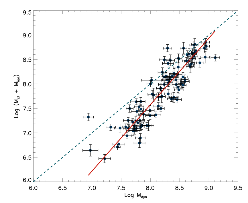
Figure 15: Comparison between $M_{cl}+M_{ion}$ and $M_{dyn}$. The continuos thick line represents the best fit to the data. The dashed line shows the one-to-one relation.

5.5.3 Dynamical masses

The dynamical masses were calculated following the expression [cf. Binney & Tremaine (1987)]:

$$M_{dyn}=10^{3}R\sigma^{2},$$ (25)

where $\sigma$ is the velocity dispersion in $\mathrm{km\ s^{-1}}$, $M_{dyn}$ is given in $M_{\odot}$ and $R$ is the cluster effective radius in parsecs (i.e. such that $1/2$ of the mass lies inside it).

To obtain an unbiased estimate of the dynamical mass a good measurement of the effective size of the ionising massive cluster is necessary. As discussed above regarding the high dispersion observations, we have evidence that many of the objects in the sample are perhaps unresolved even under very good seeing conditions. We have searched the HST database for high resolution images of objects in our sample and found only 2 HIIGx with HST WFC3 images: J091434+470207 and J093813+542825.

A quick analysis of the HST images for these two objects shows that they are only marginally resolved and have effective radius of just a few parsecs. In order to improve the small number statistics we searched the HST high resolution database for star-forming nearby objects using the same selection criteria as for the objects in this paper, and found 18 HIIGx and GEHR that also have SDSS images. Comparing the HST angular size with the Petrosian radius obtained from the SDSS u band photometry (corrected for seeing) we have found that the ionising cluster radius masured from the HST images is on average more than a factor of 5 smaller than the SDSS Petrosian radius. A more extensive analysis is performed in a forthcoming paper (Terlevich et al., in preparation). For estimating the dynamical mass we assumed that this factor applies to all HIIGx and therefore we have used a HST ‘corrected’ Petrosian radius as a proxy for the cluster radius. The values of the seeing corrected Petrosian 50 radius are listed in column (11) of Table LABEL:tab:tab05. The calculated $M_{dyn}$ is given in column (12). The masses of the clusters, both photometric, i.e. $M_{cl}+M_{ion}$ and dynamical, are large and at the same time their size is very compact. The masses range over three decades from about 2 $\times$ 10⁶ M_⊙ to 10⁹ M_⊙ while the HST corrected Petrosian radius ranges from few tens of parsecs to a few hundred parsecs.

In Figure 15 we compare the sum of $M_{cl}+M_{ion}$ with $M_{dyn}$. It is clear from the figure that the value of $M_{dyn}$, computed assuming that the Petrosian radius is on average 5 times larger than the effective radius of the ionising cluster, is slightly larger than the sum of the photometric stellar and ionized gas components particularly for the lower mass objects. Also the slope of the fit to the data has a slope of 1.3 and not 1.0. Considering the uncertainties in the determination of the three parameters involved the small level of the disagreement is surprising.

It is not clear at this stage what is the mass of the cold gas, both atomic and molecular, that remains from the starformation event. To further investigate this important question, in addition to high resolution optical and NIR images to measure the size of the ionizing clusters, high resolution observations in HI and CO or other molecular gas indicator are needed.

5.6 The metallicity – luminosity relation.

In order to test the possible existence of a metallicity - luminosity relation for HIIGx, we have performed a least squares fit for the 100 objects with direct metallicity determination in the S3 sample using the continuum luminosity as calculated from the relation given by Terlevich & Melnick (1981) and the metallicity as calculated in the above section. The results, shown in Figure 16, clearly indicate that a correlation exists albeit weak.

We have performed also a least squares fit using the H$\beta$ luminosity and the metallicity for the same sample. The results are shown in Figure 17 where a similarly weak correlation between both parameters can be seen.

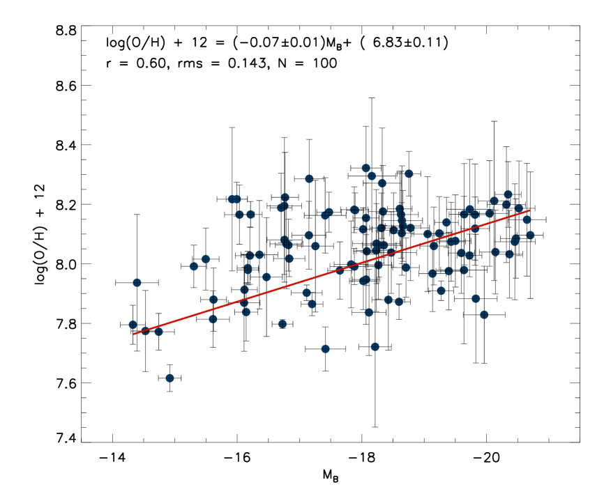
Figure 16: The continuum luminosity-metallicity relation for S3. The red line shows the best fit, which is described in the inset text.

Figure 17: The $\mathrm{H}\beta$ luminosity-metallicity relation for S3. The red line shows the best fit, which is described in the inset text.

5.7 The metallicity – equivalent width relation

We tested the possibility that a relation exists between the metallicity and the equivalent width of the H$\beta$ emission line acting as a proxy for the age of the starburst. We have performed a least squares fit to these two parameters for the S3 sample. The results are shown in Figure 18 where a trend can be seen clearly. This correlation between EW$(\mathrm{H}\beta)$ and metallicity for a large sample of HIIGx covering a wider spectrum of ages and metallicities, has already been discussed in Terlevich et al. (2004) [see their Figure 5]. They interpreted the results as being consistent with two different timescales for the evolution of HIIGx on the metallicity – EW$(\mathrm{H}\beta)$ plane. The idea is that the observed value of the EW$(\mathrm{H}\beta)$ results from the emission produced in the present burst superposed on the continuum generated by the present burst plus all previous episodes of star formation that also contributed to enhance the metallicity.

Figure 18: The EW($\mathrm{H}\beta$) - metallicity relation for S3. The red line shows the best fit, which is described in the inset text.

6 The L – $\sigma$ correlation

The main objective of this paper is to assess the validity of the $L-\sigma$ relation and its use as a distance estimator.

As discussed by e.g. Bordalo & Telles (2011), rotation and multiplicity in the sample objects can cause additional broadening of the emission lines which in turn may introduce scatter in the $L-\sigma$ relation.

In this context (Chávez et al., 2012) performed a selection based on direct visual inspection of the H$\beta$, H$\alpha$ and [OIII]$\lambda\ 4959$ and $\lambda\ 5007$ line profiles combined with the kinematic analysis mentioned in §4.2.1. At the end of this process only 69 objects (subsample S5) of the observed 128 were left with symmetric gaussian profiles and no evidence of rotation or multiplicity. This turned up as being a very expensive process in terms of observing time.

6.1 Automatic profile classification

To evaluate objectively the ‘quality’ of the emission line profiles and to avoid possible biases associated with a subjective selection of the objects such as the ones performed by Bordalo & Telles (2011) or Chávez et al. (2012) we developed a blind testing algorithm that can ‘decide’ from the high dispersion data, which are the objects that have truly gaussian profiles in their emission lines. The algorithm uses $\delta_{FWHM}(\mathrm{H}\beta)<10$ and $\delta_{flux}(\mathrm{H}\beta)<10$ as selection criteria. These quantities are defined as follows:

$$\delta_{FWHM}=\frac{\Delta_{FWHM}}{\mu_{FWHM}}\times 100,$$ (26)

where $\mu_{FWHM}$ is the mean of the FWHM as measured from a single and triple gaussian fitting to the a specific high resolution line profile and $\Delta_{FWHM}$ is the absolute value of the difference between these measurements. And

$$\delta_{flux}=\frac{\Delta_{flux}}{\mu_{flux}}\times 100,$$ (27)

where $\mu_{flux}$ is the mean of the fluxes as measured from the integration and gaussian fitting to the same spectral line in low resolution and $\Delta_{flux}$ is the absolute value of the difference between those measurements.

The rationale behind this approach is that these two quantities will measure departures from a single gaussian fitting of the actual profile. A large deviation is an indication of strong profile contamination due to second order effects such as large asymmetries and/or bright extended wings.

Figure 19 illustrates the parameters of the automatic selection. Objects inside the box delimited by a dashed line have $\delta_{flux}(\mathrm{H}\beta)<10$ and $\delta_{FWHM}(\mathrm{H}\beta)<10$. This, plus the condition $\log(\sigma)<1.8$, define the S4 sample of 93 objects.

Figure 19: Automatic profile selection. Objects inside the box delimited by a dashed line have $\delta_{flux}(\mathrm{H}\beta)<10$ and $\delta_{FWHM}(\mathrm{H}\beta)<10$. This condition plus $\log(\sigma)<1.8$ define the S4 sample of 93 objects.

Table 7: Correlation coefficients for the $L-\sigma$ relation for a range of discrimination levels in the automatic selection algorithm.

(1)	(2)	(3)	(4)	(5)
Cut Level	$\alpha$	$\beta$	rms	N
10	33.69 $\pm$ 0.22	4.67 $\pm$ 0.14	0.337	93
8	33.70 $\pm$ 0.23	4.66 $\pm$ 0.15	0.343	82
5	33.94 $\pm$ 0.26	4.51 $\pm$ 0.17	0.317	55
3	33.55 $\pm$ 0.33	4.74 $\pm$ 0.22	0.314	34
1	33.60 $\pm$ 0.49	4.63 $\pm$ 0.32	0.289	16

The $L-\sigma$ relation for the 107 objects in S3 for which we have a good estimate of their luminosity and velocity dispersion is shown in figure 20. It follows the expression:

$$\log L(\mathrm{H}\beta)=(4.65\pm 0.14)\log\sigma+(33.71\pm 0.21),$$ (28)

with an rms scatter of $\delta\log L(\mathrm{H}\beta)=0.332$.

For the 69 objects of the restricted sample (S5) we obtained:

$$\log L(\mathrm{H}\beta)=(4.97\pm 0.17)\log\sigma+(33.22\pm 0.27),$$ (29)

An important conclusion of the comparison of the results obtained from S3 and S5 is that while the $L-\sigma$ relation scatter is reduced from an rms of 0.332 to an rms of 0.25 for S5, the errors in both the slope and zero points are slightly larger for the latter as a result of reducing the number of objects by about 2/3.

Figure 20: $L-\sigma$ relation for all the HIIGx with good determination of Luminosity and $\sigma$ (S3). The inset shows the distribution of the residuals of the fit.

6.2 Further restricting the sample by the quality of the line profile fits

We have also investigated the sensitivity of the $L(\mathrm{H}\beta)-\sigma$ relation to changes in the emission line profiles as determined by the quality of the gaussian fit. The definition of quality is related to the automatic profile classification described in the previous section and illustrated in figure 19. Objects inside the box delimited by the dashed lines have $\delta_{flux}(\mathrm{H}\beta)<10$ and $\delta_{FWHM}(\mathrm{H}\beta)<10$. By adding the condition that $\log(\sigma)<1.8$ we obtain the S4 sample of 93 objects. We have selected five subsamples with increasing restricted definition of departure from a gaussian fit, i.e. with differences smaller than 10, 8, 5, 3 and 1 percent. The criteria are arbitrary and different cuts could have been justified, but the procedure was just used as a test and as such, any reasonable cut is valuable. The results of the fits are shown in table 7.

We can see from the table, that more restrictive gaussian selection still gives very similar values of the slope and the zero point of the $L(\mathrm{H}\beta)-\sigma$ relation. It achieves a small improvement in the rms but at the cost of a much reduced sample which results in a substantial increase of the errors of the slope and zero point roughly as the inverse of the square root of the number of objects.

It is interesting to compare these results with those using S3 with 107 objects some of them with profiles that clearly depart from gaussian. The least squares fit for S3 (see equation 36) gives coefficients $33.71\pm 0.21$ and $4.65\pm 0.14$ for the zero point and slope of the relation respectively. These values are very similar to those at the 10 percent cut but the rms and errors in the coefficients are smaller, consistent with a sample containing a larger number of objects.

We conclude form this exercise that the $L(\mathrm{H}\beta)-\sigma$ relation is robust against profile selection. Selecting only those objects with the best gaussian profiles makes no change in the relation coefficients but substantially increases the errors and the rms of the fit due to the reduction in the number of objects. We therefore suggest the use of the $L(\mathrm{H}\beta)-\sigma$ relation without a finer line profile selection.

Furthermore, when applying the $L(\mathrm{H}\beta)-\sigma$ distance estimator to high redshift HIIG where the data is bound to have a lower S/N, a selection based on details of the emission line profile will be difficult to perform. Ideally we would like to reduce the distance estimator scatter without reducing the number of objects, i.e. with only a small percentage of rejects from the original observed sample.

It is clear from an inspection of figure 20 (for S3) that the error bars are somehow smaller than the observed scatter in the relation, suggesting the presence of a second parameter in the correlation. As we will show below, this is indeed the case and thus it is possible to reduce substantially the scatter of the relation by including additional independent observables without a drastic reduction of the number of objects in the sample.

6.3 Search for a second parameter in the $L(\mathrm{H}\beta)-\sigma$ relation

In this section we explore the possibility that the scatter – at least part of it – in the $L(\mathrm{H}\beta)-\sigma$ relation is due to a second parameter.

Let us assume that the $L(\mathrm{H}\beta)-\sigma$ relation is a reflection of the virial theorem and a constant M/L ratio for the stellar population of these very young stellar clusters. Given that the virial theorem is bi-parametric, with the mass of the cluster depending on cluster’s velocity dispersion and size, one would expect the size of the system to be a second parameter in the $L(\mathrm{H}\beta)-\sigma$ relation.

The ionising flux in these young clusters evolve very rapidly, therefore it is also expected that age should play a role in the luminosity scatter. Thus parameters like the equivalent width of the Balmer lines or continuum colours that are good age indicators may also play a role in the scatter. Melnick et al. (1987) proposed chemical composition, in fact the oxygen abundance, as a second parameter in the $L(\mathrm{H}\beta)-\sigma$ relation.

In what follows we will analyse one by one these potential second parameters.

Table 8: Regression coefficients for S3

(1)	(2)	(3)	(4)	(5)	(6)
Parameter	$\alpha$	$\beta$	$\gamma$	rms	N
$R_{u}$	34.04 $\pm$ 0.20	3.08 $\pm$ 0.22	0.76 $\pm$ 0.13	0.261	99
$R_{g}$	34.29 $\pm$ 0.20	3.22 $\pm$ 0.22	0.59 $\pm$ 0.12	0.270	103
$R_{r}$	34.08 $\pm$ 0.21	3.29 $\pm$ 0.22	0.61 $\pm$ 0.13	0.274	101
$R_{i}$	34.08 $\pm$ 0.23	3.50 $\pm$ 0.22	0.50 $\pm$ 0.14	0.286	102
$R_{z}$	34.09 $\pm$ 0.23	3.36 $\pm$ 0.23	0.56 $\pm$ 0.14	0.282	101
$O/H$	32.16 $\pm$ 0.32	3.71 $\pm$ 0.22	0.38 $\pm$ 0.21	0.295	100
$N2$	35.60 $\pm$ 0.19	3.63 $\pm$ 0.24	0.21 $\pm$ 0.12	0.294	103
$R23$	34.47 $\pm$ 0.24	3.85 $\pm$ 0.23	0.59 $\pm$ 0.46	0.300	102
$W(H\beta)$	34.74 $\pm$ 0.23	3.73 $\pm$ 0.22	0.22 $\pm$ 0.15	0.303	107
$(u-i)$	35.08 $\pm$ 0.21	3.76 $\pm$ 0.22	0.05 $\pm$ 0.07	0.302	103

Table 9: Regression coefficients for S4.

(1)	(2)	(3)	(4)	(5)	(6)
Parameter	$\alpha$	$\beta$	$\gamma$	rms	N
$R_{u}$	34.08 $\pm$ 0.20	2.96 $\pm$ 0.25	0.81 $\pm$ 0.14	0.260	88
$R_{g}$	34.33 $\pm$ 0.20	3.07 $\pm$ 0.25	0.65 $\pm$ 0.13	0.268	90
$R_{r}$	34.09 $\pm$ 0.22	3.18 $\pm$ 0.25	0.67 $\pm$ 0.14	0.274	89
$R_{i}$	33.98 $\pm$ 0.23	3.33 $\pm$ 0.25	0.62 $\pm$ 0.17	0.285	89
$R_{z}$	34.13 $\pm$ 0.24	3.31 $\pm$ 0.25	0.57 $\pm$ 0.16	0.285	89
$O/H$	32.30 $\pm$ 0.33	3.71 $\pm$ 0.24	0.36 $\pm$ 0.24	0.298	87
$N2$	35.59 $\pm$ 0.20	3.63 $\pm$ 0.27	0.19 $\pm$ 0.14	0.299	89
$R23$	34.56 $\pm$ 0.25	3.85 $\pm$ 0.25	0.49 $\pm$ 0.50	0.304	89
$W(H\beta)$	34.77 $\pm$ 0.24	3.75 $\pm$ 0.24	0.19 $\pm$ 0.18	0.308	93
$(u-i)$	35.09 $\pm$ 0.22	3.77 $\pm$ 0.23	0.03 $\pm$ 0.08	0.305	90

Table 10: Bayesian Regression coefficients for S3

(1)	(2)	(3)	(4)	(5)	(6)
Parameter	$\alpha$	$\beta$	$\gamma$	rms	N
$R_{u}$	33.75 $\pm$ 0.37	3.36 $\pm$ 0.26	0.71 $\pm$ 0.14	0.263	99
$R_{g}$	33.84 $\pm$ 0.37	3.47 $\pm$ 0.25	0.61 $\pm$ 0.13	0.273	103
$R_{r}$	33.71 $\pm$ 0.41	3.57 $\pm$ 0.26	0.59 $\pm$ 0.14	0.277	101
$R_{i}$	33.61 $\pm$ 0.47	3.76 $\pm$ 0.25	0.52 $\pm$ 0.16	0.289	102
$R_{z}$	33.15 $\pm$ 0.46	3.47 $\pm$ 0.25	0.82 $\pm$ 0.17	0.290	101
$O/H$	30.67 $\pm$ 3.07	3.96 $\pm$ 0.26	0.51 $\pm$ 0.40	0.298	100
$N2$	34.94 $\pm$ 0.55	3.99 $\pm$ 0.28	0.14 $\pm$ 0.13	0.297	103
$R23$	33.83 $\pm$ 0.67	4.16 $\pm$ 0.26	0.75 $\pm$ 0.49	0.303	102
$W(H\beta)$	34.23 $\pm$ 0.51	4.02 $\pm$ 0.24	0.23 $\pm$ 0.17	0.305	107
$(u-i)$	34.62 $\pm$ 0.38	4.05 $\pm$ 0.24	0.04 $\pm$ 0.08	0.304	103

6.3.1 Size

If the $L(\mathrm{H}\beta)-\sigma$ correlation is a consequence of these young massive clusters being at (or close to) virial equilibrium, then the strongest candidate for a second parameter is the size of the star forming region (Terlevich & Melnick, 1981; Melnick et al., 1987). We have explored this possibility using the SDSS measured radii for our sample in all the available bands. The general form of the correlation is:

$$\log L(\mathrm{H}\beta)=\alpha+\beta\log\sigma+\gamma\log R_{i}\,$$ (30)

where $\alpha$, $\beta$ and $\gamma$ are the correlation coefficients and i runs over the SDSS bands (u, g, r, i, z). In all cases we have used the SDSS measured effective Petrosian radii and corrected for seeing also available from SDSS. Tables 8 and 9 show the correlation coefficients and the scatter obtained by means of a $\chi^{2}$ reduction procedure for the S3 and S4 samples respectively.

Consistent with what we found above regarding the profile selection, the results of the fits of the ‘10% cut’ sample S4 are not better than those of S3. Therefore in what follows we will only consider S3 taking it as the ‘benchmark’ sample.

Using the method proposed by Kelly (2007) and his publicly available IDL routines we performed a bayesian multi-linear fit. The reason to use this additional analysis is to obtain better estimates of the uncertainties in every one of the correlation coefficients. The results of the analysis are shown in table 10 for S3. Comparing these results with those obtained previously (Tables 8 and 9) it is clear that there are only small differences in the coefficients and their uncertainties which are attributable to the better treatment of errors in the bayesian procedure. The bayesian zero point tends to be smaller while the slopes tend to be slightly larger.

We have repeated the previous analysis using the values of velocity dispersion as measured from the O[III]$\lambda$ 5007 line instead of that of the $\mathrm{H}\beta$ line. The results for S3 are shown in Tables 11 and 12 for the $\chi^{2}$ reduction and the bayesian analysis respectively.

After comparing the results presented in tables 8 and 11 we found that the use of $\sigma$(O[III]) introduces only a small extra dispersion in the relation.

At this stage we conclude that the size is indeed a second parameter of the correlation and in particular the size in the u band shows the best results.

$$\begin{split}\log&L(\mathrm{H}\beta)=(3.08\pm 0.22)\log\sigma+(0.76\pm 0.13)\log(R_{u})+\\ &+(34.04\pm 0.20),\end{split}$$ (31)

with an rms scatter of $\delta\log L(\mathrm{H}\beta)=0.261$.

Still, we have to be aware that the contribution of the size to the reduction of thescatter of the correlation is limited probably due to the fact already discussed in §5.7, that the Petrosian radius is not a good estimator of the cluster dimension, but instead a measure of the size of the whole system.

6.3.2 Metallicity

Terlevich & Melnick (1981) proposed that oxygen abundance is a good indicator of the long term evolution of the system. They proposed a simple ‘closed box’ chemical evolution model with many successive cycles of star formation in which, for each cycle, evolution is traced by the $EW(\mathrm{H}\beta)$ whereas the long term evolution of the system, spanning two or more cycles, could be traced by the oxygen abundance, which then becomes a plausible second parameter in the $L(\mathrm{H}\beta)-\sigma$ correlation. When metallicity is used as a second parameter the resulting correlation is given by:

$$\log L(\mathrm{H}\beta)=\alpha+\beta\log\sigma+\gamma[12+\log\mathrm{(O/H)}]\,$$ (32)

where $\alpha$, $\beta$ and $\gamma$ are the correlation coefficients shown in Tables 8, 9, 10, 11 and 12 following the same procedure as described in the previous section for the radii. It is clear that the metallicity plays a role as a second parameter albeit relatively small. We must not forget, though, that because of the nature of the sample objects, the dynamical range of metallicity is very narrow (see Figure 14), not enough to affect significantly the $L(\mathrm{H}\beta)-\sigma$ correlation.

Table 11: Regression coefficients for S3 using $\sigma([\mathrm{OIII}])$.

(1)	(2)	(3)	(4)	(5)	(6)
Parameter	$\alpha$	$\beta$	$\gamma$	rms	N
$R_{u}$	34.44 $\pm$ 0.17	2.78 $\pm$ 0.24	0.82 $\pm$ 0.14	0.290	99
$R_{g}$	34.77 $\pm$ 0.16	2.93 $\pm$ 0.24	0.61 $\pm$ 0.13	0.303	103
$R_{r}$	34.55 $\pm$ 0.17	3.00 $\pm$ 0.24	0.64 $\pm$ 0.14	0.306	101
$R_{i}$	34.67 $\pm$ 0.18	3.23 $\pm$ 0.24	0.48 $\pm$ 0.16	0.321	102
$R_{z}$	34.53 $\pm$ 0.20	3.07 $\pm$ 0.24	0.60 $\pm$ 0.15	0.312	101
$O/H$	33.45 $\pm$ 0.24	3.45 $\pm$ 0.23	0.28 $\pm$ 0.23	0.328	100
$N2$	36.33 $\pm$ 0.15	3.28 $\pm$ 0.25	0.26 $\pm$ 0.14	0.327	103
$R23$	35.35 $\pm$ 0.18	3.52 $\pm$ 0.24	0.29 $\pm$ 0.50	0.332	102
$W(H\beta)$	35.02 $\pm$ 0.20	3.46 $\pm$ 0.23	0.35 $\pm$ 0.17	0.329	107
$(u-i)$	35.64 $\pm$ 0.17	3.51 $\pm$ 0.23	-0.02 $\pm$ 0.08	0.334	103

Table 12: Bayesian regression coefficients for S3 using $\sigma([\mathrm{OIII}])$.

(1)	(2)	(3)	(4)	(5)	(6)
Parameter	$\alpha$	$\beta$	$\gamma$	rms	N
$R_{u}$	34.29 $\pm$ 0.40	2.95 $\pm$ 0.27	0.78 $\pm$ 0.16	0.291	99
$R_{g}$	34.46 $\pm$ 0.39	3.08 $\pm$ 0.27	0.64 $\pm$ 0.15	0.304	103
$R_{r}$	34.34 $\pm$ 0.44	3.16 $\pm$ 0.27	0.62 $\pm$ 0.16	0.307	101
$R_{i}$	34.37 $\pm$ 0.50	3.40 $\pm$ 0.26	0.49 $\pm$ 0.18	0.322	102
$R_{z}$	33.75 $\pm$ 0.50	3.08 $\pm$ 0.26	0.85 $\pm$ 0.19	0.317	101
$O/H$	31.87 $\pm$ 3.41	3.57 $\pm$ 0.27	0.45 $\pm$ 0.44	0.330	100
$N2$	35.94 $\pm$ 0.56	3.49 $\pm$ 0.28	0.22 $\pm$ 0.15	0.328	103
$R23$	34.92 $\pm$ 0.71	3.72 $\pm$ 0.26	0.42 $\pm$ 0.54	0.333	102
$W(H\beta)$	34.72 $\pm$ 0.55	3.65 $\pm$ 0.24	0.35 $\pm$ 0.19	0.331	107
$(u-i)$	35.35 $\pm$ 0.38	3.70 $\pm$ 0.25	-0.03 $\pm$ 0.09	0.335	103

Table 13: Regression coefficients for S3.

(1)	(2)	(3)	(4)	(5)	(6)	(7)	(8)
Parameters	$\alpha$	$\beta$	$\gamma$	$\delta$	$\epsilon$	rms	N
$R_{u}$, $(u-i)$	33.93 $\pm$ 0.20	2.97 $\pm$ 0.22	0.91 $\pm$ 0.14	-0.16 $\pm$ 0.08	—	0.255	99
$R_{u}$, $O/H$	32.76 $\pm$ 0.24	3.10 $\pm$ 0.22	0.71 $\pm$ 0.13	0.17 $\pm$ 0.19	—	0.260	96
$R_{u}$, $N2$	33.73 $\pm$ 0.21	3.08 $\pm$ 0.22	0.88 $\pm$ 0.13	0.01 $\pm$ 0.11	—	0.247	97
$R_{u}$, $R23$	32.96 $\pm$ 0.24	3.20 $\pm$ 0.23	0.80 $\pm$ 0.13	0.91 $\pm$ 0.42	—	0.256	98
$R_{u}$, $W(H\beta)$	32.87 $\pm$ 0.23	3.00 $\pm$ 0.22	0.90 $\pm$ 0.13	0.47 $\pm$ 0.16	—	0.250	99
$W(H\beta)$, $O/H$	30.63 $\pm$ 0.38	3.69 $\pm$ 0.22	0.26 $\pm$ 0.17	0.51 $\pm$ 0.22	—	0.291	100
$W(H\beta)$, $N2$	35.38 $\pm$ 0.19	3.42 $\pm$ 0.26	0.43 $\pm$ 0.20	0.42 $\pm$ 0.16	—	0.288	103
$W(H\beta)$, $R23$	34.46 $\pm$ 0.24	3.83 $\pm$ 0.23	0.05 $\pm$ 0.19	0.51 $\pm$ 0.54	—	0.300	102
$R_{u}$, $(u-i)$, $O/H$	30.43 $\pm$ 0.31	2.90 $\pm$ 0.23	0.90 $\pm$ 0.14	-0.25 $\pm$ 0.09	0.46 $\pm$ 0.21	0.249	96
$R_{u}$, $(u-i)$, $N2$	34.17 $\pm$ 0.19	2.85 $\pm$ 0.25	0.99 $\pm$ 0.14	-0.19 $\pm$ 0.09	0.17 $\pm$ 0.13	0.241	97
$R_{u}$, $(u-i)$, $R23$	33.07 $\pm$ 0.23	3.09 $\pm$ 0.23	0.91 $\pm$ 0.14	-0.13 $\pm$ 0.08	0.75 $\pm$ 0.43	0.252	98
$R_{u}$, $W(H\beta)$, $O/H$	29.30 $\pm$ 0.33	2.95 $\pm$ 0.22	0.85 $\pm$ 0.13	0.57 $\pm$ 0.17	0.44 $\pm$ 0.19	0.244	96
$R_{u}$, $W(H\beta)$, $N2$	33.15 $\pm$ 0.22	2.79 $\pm$ 0.23	0.95 $\pm$ 0.13	0.63 $\pm$ 0.19	0.28 $\pm$ 0.13	0.233	97
$R_{u}$, $W(H\beta)$, $R23$	32.53 $\pm$ 0.25	3.07 $\pm$ 0.23	0.89 $\pm$ 0.13	0.39 $\pm$ 0.17	0.45 $\pm$ 0.46	0.249	98

Table 14: Bayesian Regression coefficients for S3.

(1)	(2)	(3)	(4)	(5)	(6)	(7)	(8)
Parameters	$\alpha$	$\beta$	$\gamma$	$\delta$	$\epsilon$	rms	N
$R_{u}$, $(u-i)$	33.60 $\pm$ 0.37	3.21 $\pm$ 0.26	0.90 $\pm$ 0.16	-0.18 $\pm$ 0.08	—	0.257	99
$R_{u}$, $O/H$	32.27 $\pm$ 2.77	3.38 $\pm$ 0.27	0.65 $\pm$ 0.15	0.20 $\pm$ 0.37	—	0.262	96
$R_{u}$, $N2$	33.16 $\pm$ 0.57	3.41 $\pm$ 0.26	0.85 $\pm$ 0.14	-0.07 $\pm$ 0.12	—	0.250	97
$R_{u}$, $R23$	32.40 $\pm$ 0.67	3.50 $\pm$ 0.26	0.77 $\pm$ 0.14	1.11 $\pm$ 0.45	—	0.258	98
$R_{u}$, $W(H\beta)$	32.46 $\pm$ 0.56	3.24 $\pm$ 0.25	0.87 $\pm$ 0.15	0.52 $\pm$ 0.17	—	0.251	99
$W(H\beta)$, $O/H$	27.89 $\pm$ 3.96	3.89 $\pm$ 0.27	0.38 $\pm$ 0.24	0.78 $\pm$ 0.47	—	0.295	100
$W(H\beta)$, $N2$	34.77 $\pm$ 0.54	3.81 $\pm$ 0.31	0.36 $\pm$ 0.25	0.31 $\pm$ 0.18	—	0.291	103
$W(H\beta)$, $R23$	33.84 $\pm$ 0.67	4.14 $\pm$ 0.26	0.02 $\pm$ 0.21	0.71 $\pm$ 0.57	—	0.303	102
$R_{u}$, $(u-i)$, $O/H$	26.05 $\pm$ 4.61	2.96 $\pm$ 0.35	0.95 $\pm$ 0.19	-0.42 $\pm$ 0.18	0.99 $\pm$ 0.60	0.260	96
$R_{u}$, $(u-i)$, $N2$	33.53 $\pm$ 0.62	3.20 $\pm$ 0.29	0.95 $\pm$ 0.15	-0.15 $\pm$ 0.10	0.06 $\pm$ 0.15	0.244	97
$R_{u}$, $(u-i)$, $R23$	32.48 $\pm$ 0.67	3.38 $\pm$ 0.27	0.89 $\pm$ 0.16	-0.14 $\pm$ 0.09	0.97 $\pm$ 0.45	0.255	98
$R_{u}$, $W(H\beta)$, $O/H$	27.19 $\pm$ 3.39	3.14 $\pm$ 0.27	0.82 $\pm$ 0.15	0.69 $\pm$ 0.23	0.65 $\pm$ 0.40	0.248	96
$R_{u}$, $W(H\beta)$, $N2$	32.69 $\pm$ 0.57	3.11 $\pm$ 0.28	0.93 $\pm$ 0.14	0.56 $\pm$ 0.22	0.19 $\pm$ 0.16	0.236	97
$R_{u}$, $W(H\beta)$, $R23$	31.97 $\pm$ 0.68	3.34 $\pm$ 0.27	0.87 $\pm$ 0.15	0.40 $\pm$ 0.20	0.66 $\pm$ 0.50	0.252	98

Table 15: Regression coefficients for S3 using $\sigma([\mathrm{OIII}])$.

(1)	(2)	(3)	(4)	(5)	(6)	(7)	(8)
Parameters	$\alpha$	$\beta$	$\gamma$	$\delta$	$\epsilon$	rms	N
$R_{u}$, $(u-i)$	34.21 $\pm$ 0.18	2.67 $\pm$ 0.23	1.03 $\pm$ 0.15	-0.26 $\pm$ 0.08	—	0.276	99
$R_{u}$, $O/H$	33.84 $\pm$ 0.19	2.81 $\pm$ 0.24	0.77 $\pm$ 0.15	0.09 $\pm$ 0.21	—	0.290	96
$R_{u}$, $N2$	34.40 $\pm$ 0.17	2.72 $\pm$ 0.24	0.90 $\pm$ 0.15	0.08 $\pm$ 0.13	—	0.280	97
$R_{u}$, $R23$	33.81 $\pm$ 0.19	2.85 $\pm$ 0.24	0.83 $\pm$ 0.14	0.56 $\pm$ 0.47	—	0.288	98
$R_{u}$, $W(H\beta)$	32.91 $\pm$ 0.22	2.73 $\pm$ 0.22	0.98 $\pm$ 0.14	0.60 $\pm$ 0.17	—	0.273	99
$W(H\beta)$, $O/H$	31.18 $\pm$ 0.33	3.43 $\pm$ 0.23	0.39 $\pm$ 0.18	0.47 $\pm$ 0.25	—	0.320	100
$W(H\beta)$, $N2$	35.79 $\pm$ 0.17	3.02 $\pm$ 0.25	0.71 $\pm$ 0.21	0.59 $\pm$ 0.16	—	0.309	103
$W(H\beta)$, $R23$	35.20 $\pm$ 0.19	3.49 $\pm$ 0.24	0.30 $\pm$ 0.20	-0.15 $\pm$ 0.58	—	0.328	102
$R_{u}$, $(u-i)$, $O/H$	30.45 $\pm$ 0.29	2.60 $\pm$ 0.23	1.02 $\pm$ 0.15	-0.35 $\pm$ 0.09	0.50 $\pm$ 0.23	0.269	96
$R_{u}$, $(u-i)$, $N2$	35.03 $\pm$ 0.16	2.41 $\pm$ 0.24	1.08 $\pm$ 0.15	-0.35 $\pm$ 0.09	0.35 $\pm$ 0.14	0.260	97
$R_{u}$, $(u-i)$, $R23$	33.90 $\pm$ 0.19	2.71 $\pm$ 0.24	1.03 $\pm$ 0.15	-0.25 $\pm$ 0.08	0.30 $\pm$ 0.46	0.275	98
$R_{u}$, $W(H\beta)$, $O/H$	29.98 $\pm$ 0.30	2.69 $\pm$ 0.23	0.93 $\pm$ 0.14	0.68 $\pm$ 0.18	0.37 $\pm$ 0.21	0.269	96
$R_{u}$, $W(H\beta)$, $N2$	33.40 $\pm$ 0.20	2.42 $\pm$ 0.23	0.98 $\pm$ 0.14	0.90 $\pm$ 0.20	0.45 $\pm$ 0.14	0.253	97
$R_{u}$, $W(H\beta)$, $R23$	33.04 $\pm$ 0.21	2.72 $\pm$ 0.23	0.96 $\pm$ 0.14	0.60 $\pm$ 0.19	-0.10 $\pm$ 0.49	0.273	98

Table 16: Bayesian regression coefficients for S3 and using $\sigma([\mathrm{OIII}])$.

(1)	(2)	(3)	(4)	(5)	(6)	(7)	(8)
Parameters	$\alpha$	$\beta$	$\gamma$	$\delta$	$\epsilon$	rms	N
$R_{u}$, $(u-i)$	34.03 $\pm$ 0.39	2.83 $\pm$ 0.26	1.02 $\pm$ 0.17	-0.29 $\pm$ 0.09	—	0.277	99
$R_{u}$, $O/H$	33.42 $\pm$ 3.08	2.96 $\pm$ 0.28	0.73 $\pm$ 0.17	0.12 $\pm$ 0.41	—	0.290	96
$R_{u}$, $N2$	34.04 $\pm$ 0.63	2.92 $\pm$ 0.27	0.89 $\pm$ 0.17	0.02 $\pm$ 0.14	—	0.281	97
$R_{u}$, $R23$	33.50 $\pm$ 0.71	3.03 $\pm$ 0.27	0.80 $\pm$ 0.16	0.70 $\pm$ 0.49	—	0.289	98
$R_{u}$, $W(H\beta)$	32.68 $\pm$ 0.63	2.85 $\pm$ 0.25	0.97 $\pm$ 0.16	0.63 $\pm$ 0.19	—	0.273	99
$W(H\beta)$, $O/H$	28.57 $\pm$ 4.40	3.52 $\pm$ 0.28	0.50 $\pm$ 0.26	0.75 $\pm$ 0.52	—	0.323	100
$W(H\beta)$, $N2$	35.39 $\pm$ 0.57	3.23 $\pm$ 0.30	0.72 $\pm$ 0.26	0.55 $\pm$ 0.19	—	0.310	103
$W(H\beta)$, $R23$	34.77 $\pm$ 0.71	3.69 $\pm$ 0.26	0.29 $\pm$ 0.23	0.02 $\pm$ 0.62	—	0.329	102
$R_{u}$, $(u-i)$, $O/H$	24.62 $\pm$ 5.03	2.53 $\pm$ 0.35	1.10 $\pm$ 0.20	-0.57 $\pm$ 0.19	1.23 $\pm$ 0.65	0.286	96
$R_{u}$, $(u-i)$, $N2$	34.68 $\pm$ 0.62	2.60 $\pm$ 0.28	1.08 $\pm$ 0.17	-0.36 $\pm$ 0.11	0.30 $\pm$ 0.16	0.261	97
$R_{u}$, $(u-i)$, $R23$	33.52 $\pm$ 0.69	2.88 $\pm$ 0.27	1.03 $\pm$ 0.17	-0.27 $\pm$ 0.09	0.46 $\pm$ 0.49	0.276	98
$R_{u}$, $W(H\beta)$, $O/H$	27.64 $\pm$ 3.87	2.73 $\pm$ 0.29	0.92 $\pm$ 0.17	0.80 $\pm$ 0.25	0.63 $\pm$ 0.46	0.272	96
$R_{u}$, $W(H\beta)$, $N2$	33.10 $\pm$ 0.62	2.56 $\pm$ 0.27	0.99 $\pm$ 0.16	0.89 $\pm$ 0.24	0.40 $\pm$ 0.17	0.254	97
$R_{u}$, $W(H\beta)$, $R23$	32.72 $\pm$ 0.73	2.85 $\pm$ 0.27	0.95 $\pm$ 0.16	0.62 $\pm$ 0.21	0.02 $\pm$ 0.53	0.274	98

We have repeated the analysis using the strong line metallicity indicators N2 and R23. The results are also given in Tables 8, 9, 10, 11 and 12. They are similar to those obtained using T_e based direct metallicity but surprisingly, showing slightly less dispersion when using N2.

Figure 21: Observed L(H$\beta$) [L(H$\beta)_{o}$] vs. L(H$\beta$) calculated using the best Bayesian multiparametric fitting corresponding to the expresion displayed on the top of the figure. The 1:1 line is shown. The inset panel shows the luminosity residuals distribution.

6.3.3 Age

The age of the starburst is also a second parameter candidate for the $L(\mathrm{H}\beta)-\sigma$ correlation. We used the $EW(\mathrm{H}\beta)$ as a starburst age indicator (Dottori, 1981; Dottori & Bica, 1981). The resulting correlation is given as:

$$\log L(\mathrm{H}\beta)=\alpha+\beta\log\sigma+\gamma\log EW(\mathrm{H}\beta)\,$$ (33)

and the coefficients are shown in Tables 8, 9, 10, 11 and 12.

Another possible age indicator is the continuum colour. We consider the (u - i) colour as a second parameter, the resulting correlation is given by:

$$\log L(\mathrm{H}\beta)=\alpha+\beta\log\sigma+\gamma(u-i)\,$$ (34)

The coefficients are also shown in Tables 8, 9, 10, 11 and 12.

From the above results, it is clear that age should play a role in the scatter of the $L(\mathrm{H}\beta)-\sigma$ correlation albeit very small. As with metallicity, by design the sample covers a narrow dynamic range of ages, consequence of the selection of equivalent widths of the emission lines, chosen in order to use for this study only bursts younger than about 5 Myr.

As already mentioned, we find that limiting the sample to objects with gaussian profiles does not improve the fit but limiting the sample to objects with log($\sigma$) $<$ 1.8, does. The second parameter with largest variance is the UV size. Including it does improve radically the fit.

It is interesting to note that in the absence of a size determination, the best second parameter is the oxygen abundance O/H (or its proxy N2 or R23) in line with the early results of Terlevich & Melnick (1981); Melnick et al. (1987); Melnick et al. (1988). This result is critical for future work with very distant systems where the Petrosian radius will be difficult to determine.

We therefore conclude that the best second parameter is the size in particular $R_{u}$. The use of the other observables [O/H, N2, R23, EW(H$\beta$), and (u - i)] also lead to a reduction of the scatter in the relation but to a lesser extent than what is achieved by using the size. Still they are useable in the absence of a size determination.

6.4 Multiparametric fits

The theoretical expectation that the emitted luminosity per unit mass in a young cluster should rapidly evolve with age and should also have some dependence on the metallicity of the stars suggests that more parameters (other than the velocity dispersion and size of the cluster, e.g. its mass) may be playing a role in the $L(\mathrm{H}\beta)-\sigma$ relation.

We have explored the possibility that a third or even a fourth parameter are present in the correlation; the general expression for the fit is:

$$\log L(\mathrm{H}\beta)=\alpha+\beta\log\sigma+\gamma A+\delta B+\epsilon C\,$$ (35)

where $\alpha$, $\beta$, $\gamma$, $\delta$ and $\epsilon$ are the correlation coefficients and A, B and C are different combinations of parameters. Tables 13 and 14 show the parameter combinations that give the least scatter in the multi-parametric correlation for the sample S3 for a $\chi^{2}$ and a Bayesian methodology respectively. Tables 15 and 16 show the results when using the [OIII]$\lambda$ 5007 velocity dispersion.

A summary of the results indicates that when the $L(\mathrm{H}\beta)-\sigma$ relation is combined with the radius in the u band, the $(u-i)$ colour and the metallicity, the scatter is significantly reduced. The best result is:

$$\begin{split}\log&L(\mathrm{H}\beta)=(2.79\pm 0.23)\log\sigma+(0.95\pm 0.13)\log R_{u}+\\ +(&0.63\pm 0.19)\log EW(H\beta)+(0.28\pm 0.13)\log N2+\\ +(&33.15\pm 0.22),\end{split}$$ (36)

with an rms scatter of $\delta\log L(\mathrm{H}\beta)=0.233$. This best solution is illustrated in Figure 21.

It seems reasonable to infer that the resulting coefficients support the scenario of a virial origin of the $L(\mathrm{H}\beta)-\sigma$ relation, in that the $\log\sigma$ coefficient is smaller than 3, the size coefficient is close to 1 and that other effects like the age and metallicity of the burst alter the virial nature of the relation.

Table 17: Regression coefficients-HDS

(1)	(2)	(3)	(4)	(5)	(6)	(7)	(8)
Parameters	$\alpha$	$\beta$	$\gamma$	$\delta$	$\epsilon$	rms	N
$R_{u}$, $(u-i)$, $O/H$	28.44	2.72	1.12	-0.23	0.66	0.256	55
$R_{u}$, $(u-i)$, $N2$	34.21	2.62	1.13	-0.19	0.25	0.258	57
$R_{u}$, $W(H\beta)$, $O/H$	27.37	2.81	1.03	0.72	0.61	0.240	57
$R_{u}$, $W(H\beta)$, $N2$	32.95	2.43	1.04	1.01	0.49	0.232	59

Table 18: Regression coefficients-UVES

(1)	(2)	(3)	(4)	(5)	(6)	(7)	(8)
Parameters	$\alpha$	$\beta$	$\gamma$	$\delta$	$\epsilon$	rms	N
$R_{u}$, $(u-i)$, $O/H$	30.84	3.09	0.85	-0.18	0.38	0.199	38
$R_{u}$, $(u-i)$, $N2$	34.80	2.85	0.84	-0.22	0.30	0.209	38
$R_{u}$, $W(H\beta)$, $O/H$	33.23	3.02	0.53	0.13	0.16	0.232	39
$R_{u}$, $W(H\beta)$, $N2$	34.29	3.04	0.72	0.07	0.13	0.216	38

6.4.1 Comparing the scatter between UVES and HDS data

We discussed in §3.2 the different setups used for the HDS and UVES observations. We show in tables 17 and 18 the regression coefficients calculated separately for both sets of observations and the combination of parameters that renders the least scatter.

It can be seen that the scatter of the HDS data is larger than that of the UVES data. We interpret this as an effect of the wider slit used in the HDS observations combined with the compact size of the sources and the excellent seeing prevailing during the observations. All these effects put together plus unavoidable fluctuations in the auto guiding procedure may have contributed to increasing the uncertainties in the observed emission line profiles.

Although a similar but smaller effect cannot at this stage be ruled out from the UVES data, given that the slit used was also larger than the seeing disk, we can conclude that the ‘true’ scatter of the relation is probably closer – if not even smaller – to that observed in the UVES data, i.e. r.m.s. $\lesssim$0.2.

7 Discussion and Conclusions

We have carefully constructed a sample of 128 compact local HII galaxies, with high equivalent widths of their Balmer emission lines, with the objective of assessing the validity of the $L({H\beta})-\sigma$ relation and its use as an accurate distance estimator. To this end we obtained high S/N high-dispersion ESO VLT and Subaru echelle spectroscopy, in order to accurately measure the ionized gas velocity dispersion. Additionally, we obtained integrated H$\beta$ fluxes from low dispersion wide aperture spectrophotometry, using the 2.1m telescopes at Cananea and San Pedro Mártir in Mexico, complemented with data from the SDSS spectroscopic survey.

After further restricting the sample to include only those systems with $\log\sigma<1.8$ and removing objects with low quality data, the remaining sample consists of 107 ‘bonafide’ HIIGx. These systems have indeed luminosities and metallicities typical of HIIGx and their position in the diagnostic diagram is typical of high excitation, low metallicity and extremely young HII regions.

Using this sample we have found that:

1. The $L(\mathrm{H}\beta)-\sigma$ relation is strong and stable against changes in the sample defined based on the characteristics of the emission line profiles. In particular we have tested the role that the ‘gaussianity’ of the line profile plays in the relation. This was tested to destruction with both objective and subjective methods of profile classification and assessment to define several subsets.

   In agreement with previous work we find that the $L(\mathrm{H}\beta)-\sigma$ relation for HIIGx with gaussian emission line profiles has a smaller scatter than that of the complete sample. On the other hand this is achieved at the cost of substantially reducing the sample. The rejected fraction in Bordalo & Telles (2011) or Chávez et al. (2012) is close to or larger than 50% which is not compensated by the gain in rms. The use of the complete sample, i.e. without a profile classification, is a far more practical proposal given that, in order to perform a proper selection of gaussian profiles, we need data that have S/N and resolution much higher than that required to measure just the FWHM. Therefore it is far more costly in terms of observing time and instrumentation requirements to determine departures from gaussianity than to just accurately measure the FWHM of an emission line. It is shown in section 6.1 that while the r.m.s. errors are indeed reduced on the fits to the subset of HIIGx with Gaussian profiles, the value of the coefficients hardly change at all, although their errors are substantially larger than those of the complete sample.

   In conclusion, selecting the best gaussian profiles improves the rms but at a very heavy cost in terms of rejects and hence of telescope time, which is neither practical nor justified for a distance estimator.

   Therefore, the use of the full sample limited only by the $\log\sigma<1.8$ selection is strongly recommended. Our best $L(\mathrm{H}\beta)-\sigma$ relation is:

   $${\log L(\mathrm{H}\beta)=4.65\log\sigma+33.71\;,}$$

   with an rms scatter of ${\delta\log L(\mathrm{H}\beta)=0.332}$.

2. We searched for the presence of a second parameter in the $L(\mathrm{H}\beta)-\sigma$ relation. We found that using as second parameter either size, oxygen abundance O/H or its proxy N2 or R23, EW or continuum colour the scatter is considerably reduced. Including the size as a second parameter produces the best fits, and among them the size in the u-band shows the smallest scatter,

   $$\log L(\mathrm{H}\beta)=3.08\log\sigma+0.76\log R_{u}+34.04\;,$$

   with an rms scatter of $\delta\log L(\mathrm{H}\beta)=0.261$.

   This result points clearly to the existence of a Fundamental Plane in HIIGx suggesting that the main mechanism of line broadening is linked to the gravitational potential of the young massive cluster. It is important to underline that in the absence of a size measurement, the best second parameter is the abundance O/H or its proxy N2 or R23, a result that is crucial for the application to very distant systems where the size will be difficult to determine.

3. We also investigated which parameters in addition to the size can further reduce the scatter. We found, using multi parametric fits , that including as a third parameter the $(u-i)$ colour or the equivalent width, and as a fourth parameter the metallicity does significantly reduce the scatter.

   Our best multiparametric estimator is:
   

   $$\log L(\mathrm{H}\beta)=2.79\log\sigma+0.95\log R_{u}+0.63\log EW(H\beta)+$$

   $$0.28\log N2+33.15$$

   with an rms scatter of $\delta\log L(\mathrm{H}\beta)=0.233$.
   

   The argument could be sustained that the value of the coefficients of the fit provides further support for the virial origin of the $L(\mathrm{H}\beta)-\sigma$ relation since the $\log\sigma$ coefficient is smaller than 3. It is quite possible that such virial nature is altered by other effects like the age (EW) and metallicity (N2) of the burst. Thus the coefficients in the best estimator (see equation (36)) are very close to what is expected from a young virialized ionising cluster and, perhaps even more relevant, the sum of the stellar and ionised gas masses of the cluster are similar to the dynamical mass estimated with the HST ‘corrected’ Petrosian radius.

   We conclude that the evidence strongly points to gravity as the main mechanism for the broadening of the emission lines in these very young and massive clusters.

   The masses of the clusters, both photometric and dynamical, are very large while their size is very compact. Their ranges cover three decades from about 2 $\times$ 10⁶ M_⊙  to 10⁹ M_⊙. Their HST corrected Petrosian radius range from a few tens of parsecs to a few hundred parsecs. To further investigate this important property of the HIIGx and its impact on the distance estimator it is crucial to secure high resolution optical and NIR images of this sample of objects.

4. Bayesian and $\chi^{2}$ fits to the $L(\mathrm{H}\beta)-\sigma$ correlation give similar results.

5. The application of the $L(\mathrm{H}\beta)-\sigma$ distance estimator to HIIGx at cosmological distances, where the size would be difficult to determine, will require the use of a metallicity indicator and the EW of the Balmer lines as a second and third parameter. According to our findings, this will result in a predictor with $\delta\log L(\mathrm{H}\beta)\sim 0.3$ using either $\sigma(H\beta)$ or the easier to determine $\sigma[OIII]$.

6. Given that the $L(\mathrm{H}\beta)-\sigma$ relation is basically a correlation between the ionising flux, produced by the massive stars, and the velocity field produced by the star and gas potential well, the existence of a narrow $L(\mathrm{H}\beta)-\sigma$ relation puts strong limits on the possible changes in the IMF. Any systematic variation in the IMF will affect directly the M/L ratio and therefore the slope and/or zero point of the relation. A change of 0.1 in the slope of the IMF would be reflected in a change in luminosity scale of the $L(\mathrm{H}\beta)-\sigma$ relation of about $\log L(\mathrm{H}\beta)\sim\ 0.2$. This seems to be too large for our found correlation.

7. An important aspect to remark is that the design of our complete selection criteria guarantees homogeneous samples at all redshifts in the sense that the imposed EW limit guarantees a sample younger than a certain age and relatively free of contamination by older populations, the upper limit in $\sigma$ guarantees a sample limited in luminosity and the diagnostic diagram selection guarantees that they are starbursts. The limitation in $\sigma$ is particularly important given that this criterion should remove biases associated with samples in which the mean luminosity changes with distance (Malmquist bias). Any dependence of the luminosity in parameters like age and metallicity are included in the multiparametric fits.

   Finally, we envisage observations of HIIGx having a limiting $\sigma$ of 63 km/s or equivalently an $\mathrm{H}\alpha\$ luminosity less than $3\times 10^{43}$ erg/s at z $\sim$ 2 to 3 with enough S/N with present instrumentation. They will require exposure times of about 1.5 to 3 hours in an instrument like X-SHOOTER at the VLT in ESO to obtain line profiles with enough S/N to determine FWHM with less than 10% rms error. This in turn will allow us to measure the local expansion rate of the Universe, $H_{0}$, to a percent precision which is a prerequisite for independent constraints on the mass-energy content and age of the Universe as well as to map its behaviour by using several independent yet accurate tracers of the cosmic expansion over the widest possible range of redshift.

Appendix A Profile fits to the high resolution H$\beta$ lines.

We have used three independent fit procedures for each object.

1. [(a)]

2. A single gaussian fit to the line using the gaussfit IDL routine.

3. Two different gaussians using the arm_asymgaussfit routine in order to explore possible asymmetries.

4. Three separate gaussians using the arm_multgaussfit routine to investigate the role of the extended ‘non-gaussian’ wings. For this case we constructed a grid of parameters to use as seeds for the routine, as described in the main text.

In Figure 22 we show the UVES instrumental profile and its gaussian fit obtained from the OI 5577 Å sky line. Figures A2 to A11 show the best fits for the H$\beta$ lines. Each plot presents the fits to a different HIIGx. The upper panel shows the three independent fits while the lower panel shows their residuals. The insets indicate the results of the fits and the distribution resulting from the Montecarlo simulation used to estimate the errors in the FWHM (see main text).

Figure 33 shows the HDS instrumental profile and its gaussian fit, obtained from the OI 5577 Å sky line. Figures A13 to A24 show the best fits corresponding to the HDS observations. The details are like those for the UVES spectra.

Figure 22: VLT-UVES instrumental profile and its gaussian fit, as obtained from the OI 5577 Å sky line. The observed line is shown in black and the gaussian fit in red. This, as all the following profiles, is shown in a 20 Å wide window.

Figure 23: H$\beta$ lines best fits for VLT UVES data. The observed $\mathrm{H}\beta$ line and the three different fits are shown in a 20 Å wide window for each object as labelled. Upper panel: The single gaussian fit is indicated by a dashed line (thick black),the asymmetric gaussian fit is indicated by a dash-dotted line (blue) and the three separate gaussians fit is indicated by long-dashed lines (red) with its total fit shown by a dash-double-dotted line (yellow); the parameters of the fits are listed in the top left corner. Lower panel: Shows the residuals from the fitting procedures following the same colour code with crosses for the single gaussian fit and continuous lines both for the asymmetric and three gaussian fits. The inset shows the results from the Montecarlo simulation to estimate the errors in the FWHM of the best fit. Details are described in the main text.

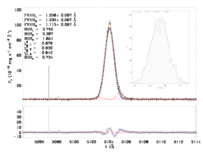
(a) J051519-391741

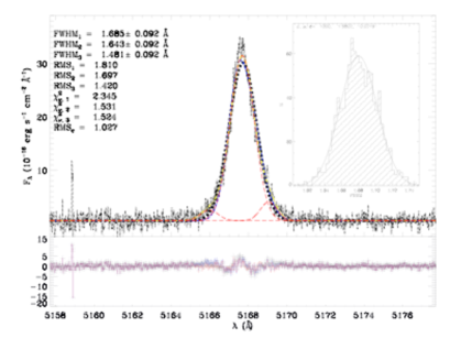
(b) J074806+193146

(c) J074947+154013

(d) J080000+274642

Figure 24: H$\beta$ lines best fits continued.

(a) J081403+235328

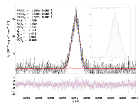
(b) J082520+082723

(c) J082520+082723

(d) J082722+202612

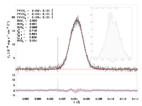
(e) J083946+140033

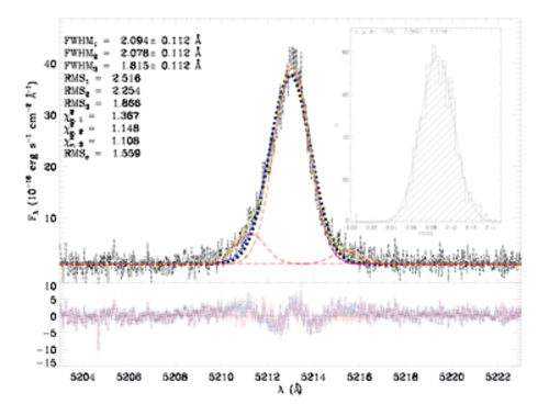
(f) J084000+180531

Figure 25: H$\beta$ lines best fits continued.

(a) J084219+300703

(b) J084414+022621

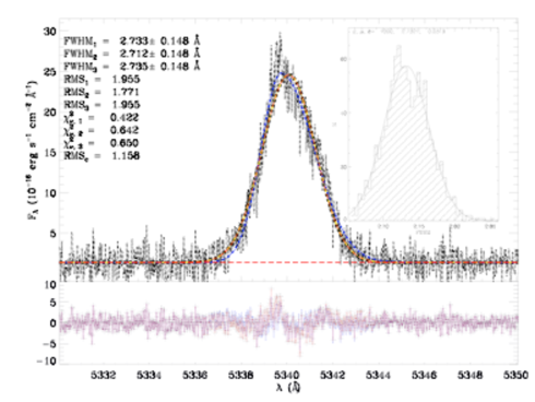
(c) J090418+260106

(d) J090506+223833

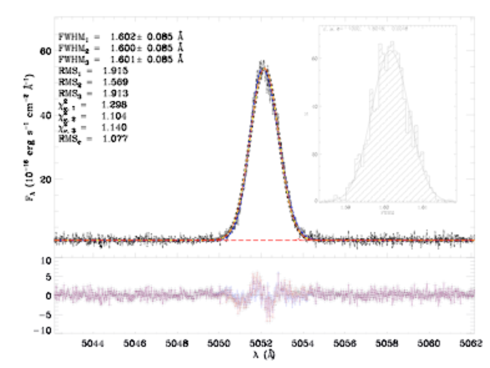
(e) J090531+033530

(f) J091652+003113

Figure 26: H$\beta$ lines best fits continued.

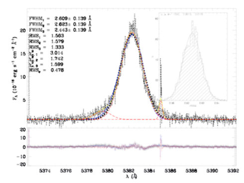
(a) J092749+084037

(b) J092918+002813

(c) J093424+222522

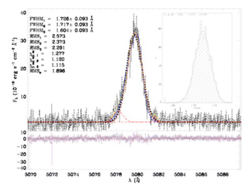
(d) J094000+203122

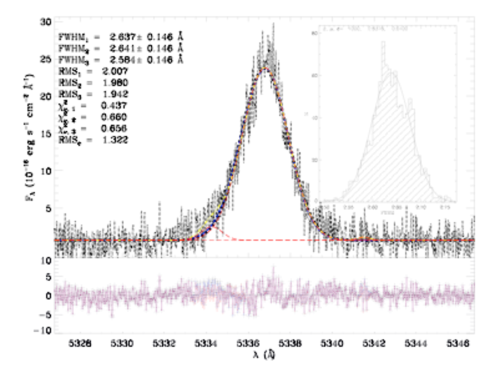
(e) J095023+004229

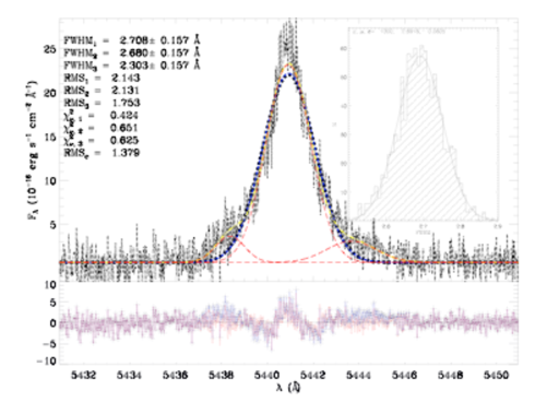
(f) J095226+021759

Figure 27: H$\beta$ lines best fits continued.

(a) J100720+193349

(b) J101042+125516

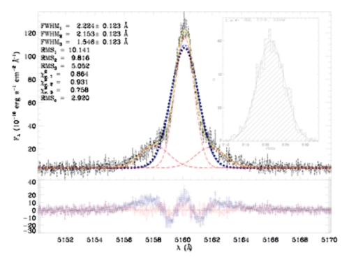
(c) J101042+125516

(d) J101136+263027

(e) J101430+004755

(f) J101430+004755

Figure 28: H$\beta$ lines best fits continued.

(a) J102732-284201

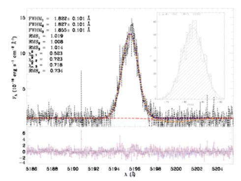
(b) J103412+014249

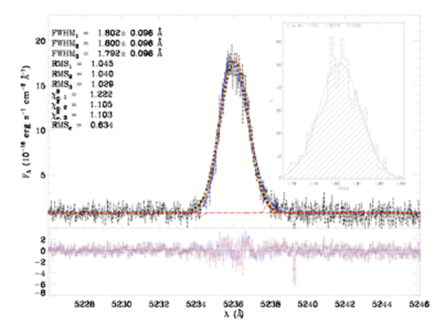
(c) J103726+270759

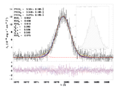
(d) J104755+073951

(e) J105040+342947

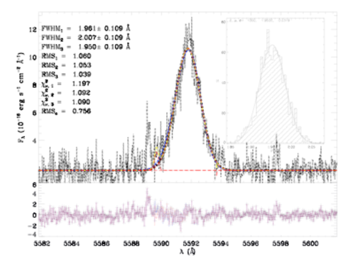
(f) J105210+032713

Figure 29: H$\beta$ lines best fits continued.

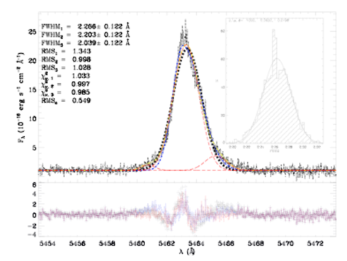
(a) J105331+011740

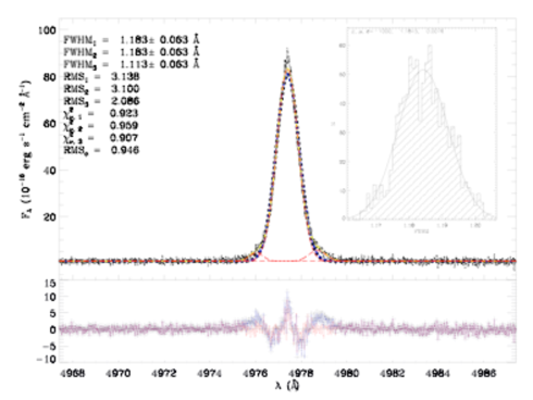
(b) J110838+223809

(c) J114212+002003

(d) J121329+114056

(e) J121717-280233

(f) J125305-031258

Figure 30: H$\beta$ lines best fits continued.

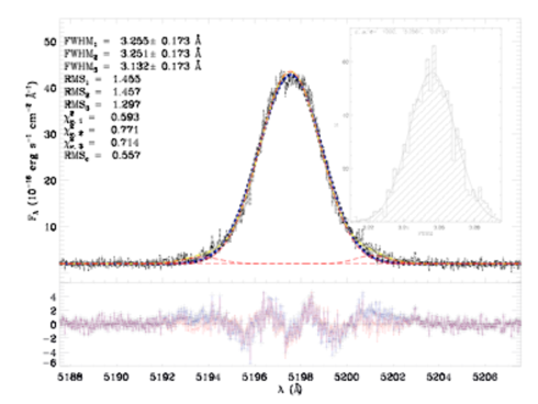
(a) J130119+123959

(b) J131235+125743

(c) J132347-013252

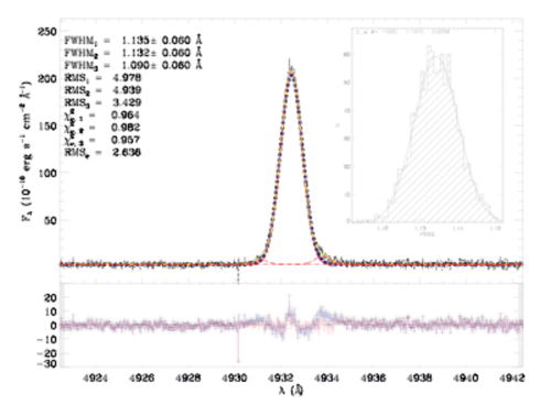
(d) J132549+330354

(e) J133708-325528

(f) J134531+044232

Figure 31: H$\beta$ lines best fits continued.

(a) J142342+225728

(b) J144805-011057

(c) J162152+151855

(d) J171236+321633

(e) J192758-413432

(f) J211527-075951

Figure 32: H$\beta$ lines best fits continued.

(a) J212043+010006

(b) J221823+003918

(c) J222510-001152

(d) J222510-001152

Figure 33: Same as Figure 22 for the Subaru HDS data.

Figure 34: Same as Figure A2 for the Subaru HDS data.

(a) J001647-104742

(b) J002339-094848

(c) J002425+140410

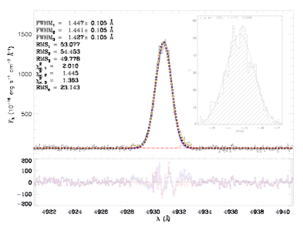
(d) J002425+140410

Figure 35: H$\beta$ lines best fits continued.

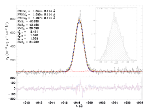
(a) J003218+150014

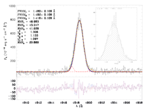
(b) J003218+150014

(c) J005147+000940

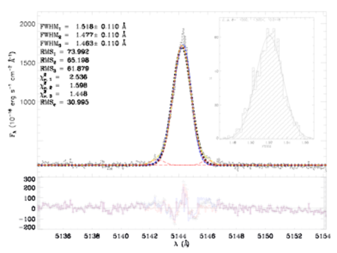
(d) J005602-101009

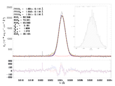
(e) J013258-085337

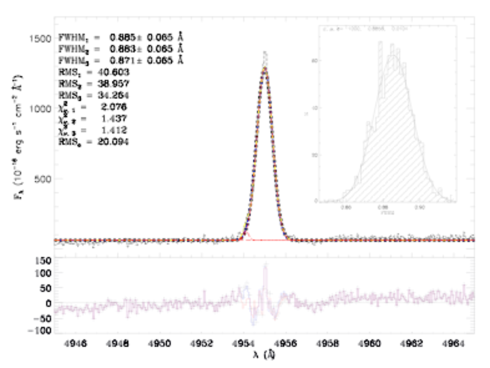
(f) J013344+005711

Figure 36: H$\beta$ lines best fits continued.

(a) J014137-091435

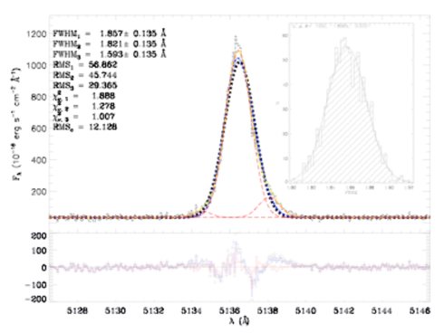
(b) J014707+135629

(c) J021852-091218

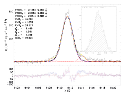
(d) J022037-092907

(e) J024052-082827

(f) J024453-082137

Figure 37: H$\beta$ lines best fits continued.

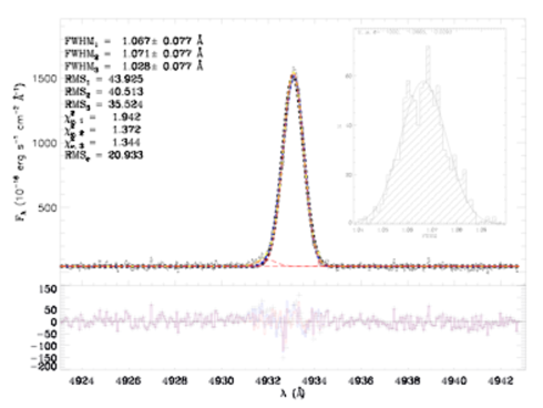
(a) J025426-004122

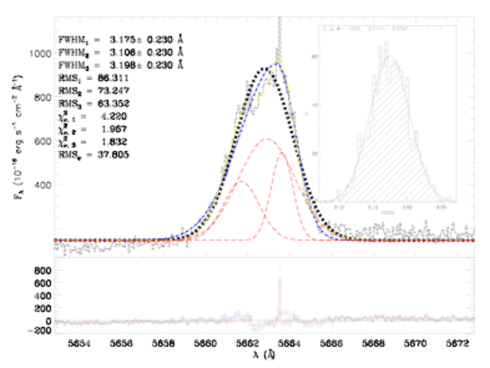
(b) J030321-075923

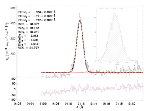
(c) J031023-083432

(d) J033526-003811

(e) J040937-051805

(f) J080619+194927

Figure 38: H$\beta$ lines best fits continued.

(a) J081334+313252

(b) J081420+575008

(c) J081737+520236

(d) J082530+504804

(e) J084029+470710

(f) J084220+115000

Figure 39: H$\beta$ lines best fits continued.

(a) J084527+530852

(b) J084634+362620

(c) J085221+121651

(d) J091434+470207

(e) J091640+182807

(f) J093006+602653

Figure 40: H$\beta$ lines best fits continued.

(a) J093813+542825

(b) J094252+354725

(c) J094254+340411

(d) J094809+425713

(e) J095000+300341

(f) J095131+525936

Figure 41: H$\beta$ lines best fits continued.

(a) J095227+322809

(b) J095545+413429

(c) J100746+025228

(d) J101036+641242

(e) J101157+130822

(f) J101458+193219

Figure 42: H$\beta$ lines best fits continued.

(a) J102429+052451

(b) J103328+070801

(c) J103509+094516

(d) J104457+035313

(e) J104554+010405

(f) J104653+134645

Figure 43: H$\beta$ lines best fits continued.

(a) J104723+302144

(b) J105032+153806

(c) J105741+653539

(d) J212332-074831

(e) J214350-072003

(f) J220802+131334

Figure 44: H$\beta$ lines best fits continued.

(a) J224556+125022

(b) J225140+132713

(c) J230117+135230

(d) J230123+133314

(e) J230703+011311

(f) J231442+010621

Figure 45: H$\beta$ lines best fits continued.

(a) J232936-011056

References

- Abazajian et al. (2009) Abazajian K. N., Adelman-McCarthy J. K., Agüeros M. A., Allam S. S., Allende Prieto C., An D., Anderson K. S. J., Anderson S. F., Annis J., Bahcall N. A., et al. 2009, ApJS, 182, 543
- Basilakos & Plionis (1998) Basilakos S., Plionis M., 1998, MNRAS, 299, 637
- Basilakos & Plionis (2006) Basilakos S., Plionis M., 2006, MNRAS, 373, 1112
- Bergeron (1977) Bergeron J., 1977, ApJ, 211, 62
- Binney & Tremaine (1987) Binney J., Tremaine S., 1987, Galactic dynamics
- Bordalo & Telles (2011) Bordalo V., Telles E., 2011, ApJ, 735, 52
- Bradley et al. (2006) Bradley T. R., Knapen J. H., Beckman J. E., Folkes S. L., 2006, A&A, 459, L13
- Calzetti et al. (2000) Calzetti D., Armus L., Bohlin R. C., Kinney A. L., Koornneef J., Storchi-Bergmann T., 2000, ApJ, 533, 682
- Chávez et al. (2012) Chávez R., Terlevich E., Terlevich R., Plionis M., Bresolin F., Basilakos S., Melnick J., 2012, MNRAS, 425, L56
- Copetti et al. (1986) Copetti M. V. F., Pastoriza M. G., Dottori H. A., 1986, A&A, 156, 111
- Courteau & van den Bergh (1999) Courteau S., van den Bergh S., 1999, AJ, 118, 337
- Dekker et al. (2000) Dekker H., D’Odorico S., Kaufer A., Delabre B., Kotzlowski H., 2000, in M. Iye & A. F. Moorwood ed., Society of Photo-Optical Instrumentation Engineers (SPIE) Conference Series Vol. 4008 of Society of Photo-Optical Instrumentation Engineers (SPIE) Conference Series, Design, construction, and performance of UVES, the echelle spectrograph for the UT2 Kueyen Telescope at the ESO Paranal Observatory. pp 534–545
- Díaz et al. (2000) Díaz A. I., Álvarez M. Á., Terlevich E., Terlevich R., Sánchez Portal M., Aretxaga I., 2000, MNRAS, 311, 120
- Dottori (1981) Dottori H. A., 1981, Ap&SS, 80, 267
- Dottori & Bica (1981) Dottori H. A., Bica E. L. D., 1981, A&A, 102, 245
- Freedman et al. (2012) Freedman W. L., Madore B. F., Scowcroft V., Burns C., Monson A., Persson S. E., Seibert M., Rigby J., 2012, ApJ, 758, 24
- García–Vargas et al. (1995) García–Vargas M. L., Bressan A., Díaz A. I., 1995, A&AS, 112, 13
- García-Díaz et al. (2008) García-Díaz M. T., Henney W. J., López J. A., Doi T., 2008, Revista Mexicana de Astronomia y Astrofisica, 44, 181
- González-Delgado et al. (1999) González-Delgado R. M., Leitherer C., Heckman T. M., 1999, ApJS, 125, 489
- Guzmán et al. (1996) Guzmán R., Koo D. C., Faber S. M., Illingworth G. D., Takamiya M., Kron R. G., Bershady M. A., 1996, ApJ, 460, L5
- Hopkins et al. (2002) Hopkins A. M., Schulte-Ladbeck R. E., Drozdovsky I. O., 2002, AJ, 124, 862
- Jarosik et al. (2011) Jarosik N., Bennett C. L., Dunkley J., Gold B., Greason M. R., Halpern M., Hill R. S., Hinshaw G., Kogut A., Komatsu E., Larson D., Limon M., Meyer S. S., Nolta M. R., Odegard N., Page L., Smith K. M., Spergel D. N., Tucker G. S., Weiland J. L., 2011, ApJS, 192, 14
- Kelly (2007) Kelly B. C., 2007, ApJ, 665, 1489
- Kennicutt & Evans (2012) Kennicutt R. C., Evans N. J., 2012, ARA&A, 50, 531
- Kennicutt et al. (1989) Kennicutt Jr. R. C., Edgar B. K., Hodge P. W., 1989, ApJ, 337, 761
- Kewley et al. (2001) Kewley L. J., Dopita M. A., Sutherland R. S., Heisler C. A., Trevena J., 2001, ApJ, 556, 121
- Koo et al. (1995) Koo D. C., Guzman R., Faber S. M., Illingworth G. D., Bershady M. A., Kron R. G., Takamiya M., 1995, ApJ, 440, L49
- Kunth & Östlin (2000) Kunth D., Östlin G., 2000, A&A Rev., 10, 1
- Leitherer & Heckman (1995) Leitherer C., Heckman T. M., 1995, ApJS, 96, 9
- Leitherer et al. (1999) Leitherer C., Schaerer D., Goldader J. D., González Delgado R. M., Robert C., Kune D. F., de Mello D. F., Devost D., Heckman T. M., 1999, ApJS, 123, 3
- Lynden-Bell (1971) Lynden-Bell D., 1971, MNRAS, 155, 119
- Melnick et al. (1987) Melnick J., Moles M., Terlevich R., Garcia-Pelayo J.-M., 1987, MNRAS, 226, 849
- Melnick et al. (1988) Melnick J., Terlevich R., Moles M., 1988, MNRAS, 235, 297
- Melnick et al. (2000) Melnick J., Terlevich R., Terlevich E., 2000, MNRAS, 311, 629
- Noguchi et al. (2002) Noguchi K., Aoki W., Kawanomoto S., Ando H., Honda S., Izumiura H., Kambe E., Okita K., Sadakane K., Sato B., Tajitsu A., Takada-Hidai T., Tanaka W., Watanabe E., Yoshida M., 2002, PASJ, 54, 855
- Oey & Clarke (1998) Oey M. S., Clarke C. J., 1998, AJ, 115, 1543
- Olofsson (1995) Olofsson K., 1995, A&AS, 111, 57
- Osterbrock (1988) Osterbrock D. E., 1988, PASP, 100, 412
- Osterbrock (1989) Osterbrock D. E., 1989, Astrophysics of gaseous nebulae and active galactic nuclei
- Pagel et al. (1979) Pagel B. E. J., Edmunds M. G., Blackwell D. E., Chun M. S., Smith G., 1979, MNRAS, 189, 95
- Pagel et al. (1992) Pagel B. E. J., Simonson E. A., Terlevich R. J., Edmunds M. G., 1992, MNRAS, 255, 325
- Pettini et al. (1998) Pettini M., Kellogg M., Steidel C. C., Dickinson M., Adelberger K. L., Giavalisco M., 1998, ApJ, 508, 539
- Plionis et al. (2011) Plionis M., Terlevich R., Basilakos S., Bresolin F., Terlevich E., Melnick J., Chavez R., 2011, MNRAS, pp 1237–+
- Riess et al. (2011) Riess A. G., Macri L., Casertano S., Lampeit H., Ferguson H. C., Filippenko A. V., Jha S. W., Li W., Chornock R., Silverman J. M., 2011, ApJ, 730, 119
- Rosa-González et al. (2002) Rosa-González D., Terlevich E., Terlevich R., 2002, MNRAS, 332, 283
- Rowan-Robinson (1968) Rowan-Robinson M., 1968, MNRAS, 138, 445
- Salpeter (1955) Salpeter E. E., 1955, ApJ, 121, 161
- Sato et al. (2002) Sato B., Kambe E., Takeda Y., Izumiura H., Ando H., 2002, PASJ, 54, 873
- Schmidt (1968) Schmidt M., 1968, ApJ, 151, 393
- Searle & Sargent (1972) Searle L., Sargent W. L. W., 1972, ApJ, 173, 25
- Siegel et al. (2005) Siegel E. R., Guzmán R., Gallego J. P., Orduña López M., Rodríguez Hidalgo P., 2005, MNRAS, 356, 1117
- Storchi-Bergmann et al. (1994) Storchi-Bergmann T., Calzetti D., Kinney A. L., 1994, ApJ, 429, 572