Dynamic programming
using radial basis functions
Abstract.
We propose a discretization of the optimality principle in dynamic programming based on radial basis functions and Shepard’s moving least squares approximation method. We prove convergence of the approximate optimal value function to the true one and present several numerical experiments.
Oliver Junge and Alex Schreiber
Center for Mathematics
Technische Universität München
85747 Garching bei München
1. Introduction
For many optimal control problems, solutions can elegantly be characterized and computed by dynamic programming, i.e. by solving a fixed point equation, the Bellman equation, for the optimal value function of the problem. For every point in the state space of the underlying problem, this function yields the optimal cost associated to this initial condition. At the same time, the value function allows to construct an optimal controller in feedback form, enabling a robust stabilization of a possibly unstable nominal system. This controller not only yields optimal cost trajectories, but also a maximal domain of stability for the closed loop system.
The generality and flexibility of dynamic programming, however, comes at a price: Since in many cases, closed form solutions of the optimality principle are not available, numerical approximations have to be sought. This typically hinders the treatment of problems with higher dimensional state spaces, since the numerical effort scales exponentially in its dimension (Bellman’s curse of dimension). Early works on numerical schemes for the related Hamilton-Jacobi(-Bellman) equations [5, 2, 9, 6] were based on finite difference or finite element type space discretizations with interpolation type projection operators. Based on these, higher order [10, 11] and adaptive schemes [14, 15] have been developed, as well as interpolation based approaches for certain systems in dimensions 3-5 [7]. While in these works a simple (“value”) iteration is used in order to solve the fixed point problem, one-pass methods reminiscent of Dijkstra’s shortest path algorithm can be employed in order to solve the discrete problem more efficiently [23, 19, 18, 16]. Similar savings can be obtained by exploiting the fact that the problem becomes linear in the max-plus algebra [22].
In [8, 17, 1], radial basis functions have been proposed in order to space-discretize time-dependent Hamilton-Jacobi(-Bellman) equations by collocation. The appealing feature of this “meshfree” approach is its simplicity: The discretization is given by a set (e.g. a grid) of points in phase space which serve as the centers for the basis functions. In comparison to, e.g., finite element methods, no additional geometric information has to be computed. Note, however, that per se this does not avoid the curse of dimension.
In this manuscript, we consider a discrete time optimal control problem (which can be obtained from some HJB equation by a discretization in time with fixed time step) and show that using radial basis functions in combination with a least squares type projection (aka Shepard’s method) one obtains a simple, yet general scheme for the numerical solution of the problem which also allows for a simple convergence theory (which is not given in the above mentioned works). After a brief review on radial basis functions in Section 3, we prove convergence of the approximate value function to the true one as the fill distance of the discrete node set goes to zero (Section 4) and consider several numerical experiments (Section 5). The Matlab codes for these examples can be downloaded from the homepages of the authors.
2. Problem statement
We consider a discrete time control system
| (1) |
with a continuous map on compact sets , , , as phase and control space, respectively. In addition, we are given a continuous cost function and a compact target set and we assume that is bounded from below by a constant for and all .
Our goal is to design a feedback law , , that stabilizes the system in the sense that discrete trajectories for the closed loop system reach in a finite number of steps for starting points in a maximal subset . In many cases, one also wants to construct such that the accumulated cost
is minimized. In order to construct such a feedback, we employ the optimality principle, cf. [3, 4],
| (2) |
where is the (optimal) value function, with boundary conditions and . Using , we define a feedback by
whenever the minimum exists, e.g. if is continuous.
The Kružkov transform.
Typically, some part of the state space will not be controllable to the target set . By definition, for points in this part of . An elegant way to deal (numerically) with the fact that might attain the value , is by the (or more precisely one variant of the) Kružkov transform , where we set , cf. [20]. After this transformation, the optimality principle (2) reads
the boundary conditions transform to and . The right hand side of this fixed point equation yields the Bellman operator
| (3) |
on the Banach space , where
By standard arguments and since we assumed to be bounded from below by outside of the target set we obtain with
| (4) |
i.e. we have by the Banach fixed point theorem
Lemma 1.
The Bellman operator is a contraction and thus possesses a unique fixed point.
3. Approximation with radial basis functions
Only in simple or special cases (e.g. in case of a linear-quadratic problem), can be expressed in closed form. In general, we need to approximate it numerically. Here, we are going to use radial basis functions for this purpose, i.e. functions of the form on some set of nodes. We assume the shape function to be nonnegative, typical examples include the Gaussian and the Wendland functions , cf. [25, 12], with an appropriate polynomial. The shape parameter controls the “width” of the radial basis functions and has to be chosen rather carefully. In case that the shape function has compact support, we will need to require that the supports of the cover .
3.1. Interpolation.
One way to use radial basis functions for approximation is by (“scattered data”) interpolation: We make the ansatz
for the approximate fixed point of (3) and require to fulfill the interpolation conditions for prescribed values . The coefficient vector is then given by the solution of the linear system with and .
Formally, for some function , we can define its interpolation approximation by
where the are cardinal basis functions associated with the nodes , i.e. a nodal basis with and for . Note that depends linearly on .
3.2. Weighted least squares.
Given some approximation space , , , , , and a weight function , we define the discrete inner product
for with induced norm . The weighted least squares approximant of some function is then defined by minimizing . The solution is given by , where the optimal coefficient vector solves the linear system with Gram matrix and .
3.3. Moving least squares.
When constructing a least squares approximation to some function at , it is often natural to require that only the values at some nodes close to should play a significant role. This can be modeled by introducing a moving weight function , where is small if is large. In the following, we will use a radial weight
where is the shape function introduced before. The corresponding discrete inner product is
The moving least squares approximation of some function is then given by , where is minimizing . The optimal coefficient vector is given by the solution of the Gram system with and .
3.4. Shepard’s method
We now simply choose as approximation space. Then the Gram matrix is and the right hand side is . Thus we get , where
| (5) |
We define the Shepard approximation of as
Note again that depends linearly on . What is more, for each , is a convex combination of the values , since for all .
Shepard’s method has several advantages over interpolation: (a) Computing in a finite set of points only requires a matrix-vector product (in contrast to a linear solve for interpolation), (b) the discretized Bellman operator remains a contraction, since the Shepard operator is non-expanding (cf. Lemma 2 in the next section), and (c) the approximation behavior for an increasing number of nodes is more favorable, as we will outline next.
3.5. Stationary vs. non-stationary approximation
The number
is called the fill distance of in , while
is the separation distance. The fill distance is the radius of the largest ball inside that is disjoint from .
In non-stationary approximation with radial basis functions, the shape parameter is kept constant while the fill distance goes to . Non-stationary interpolation is convergent:
Theorem 1 ([12], Theorem 15.3).
Assume that the Fourier transform of fulfills
for some constants . In addition, let and be integers with and , and let . Also suppose that satisfies with sufficiently small fill distance. Then for any we have
where is the so-called mesh ratio for .
On the other hand, stationary interpolation, i.e. letting shrink to along with does not converge (for a counter example see [12], Example 15.10).
For Shepard’s method instead of interpolation, though, the exact opposite holds: Non-stationary approximation does not converge (cf. [12], Ch. 24), while stationary approximation does, as we will recall in Lemma 3 below. In practice, this is an advantage, since we can keep the associated matrices sparse.
4. Discretization of the optimality principle
We now want to compute an approximation to the fixed point of the Bellman operator (3) by value iteration, i.e. by iterating on some initial function . We would like to perform this iteration inside some finite dimensional approximation space , i.e. after each application of , we need to map back into .
Interpolation
Choosing , we define the Bellman interpolation operator to be
In general, the operator is expansive and not necessarily monotone. For that reason, one cannot rely on the iteration with to be convergent (although in most of our numerical experiments it turned out to converge) and move our focus towards the value iteration with Shepard’s method.
Shepard’s method.
With (cf. (5)), we define the Bellman-Shepard operator as
Explicitly, the value iteration reads
| (6) |
where, as mentioned, some initial function has to be provided.
Lemma 2.
The Shepard operator has norm .
Proof.
Since, by assumption, the are nonnegative and, as mentioned above, for each , is a convex combination of the values , we have for each
so that . Moreover, for constant one has . ∎
As a composition of the contraction and the Shepard operator , we get
Theorem 2.
The Bellman-Shepard operator is a contraction, thus the iteration (6) converges to the unique fixed point of .
Convergence for decreasing fill distance
Assume we are given a Lipschitz function and a sequence of sets of nodes with fill distances . We consider the Shepard operators associated with the sets and shape parameters for some constant . Under the assumption that we get convergence of the respective Shepard approximations to as shown in the following result, which is a minor generalization of the statement preceding theorem 25.1 in [12] from functions to Lipschitz functions. Here, we consider only shape functions with compact support.
Lemma 3.
Let and be Lipschitz continuous with Lipschitz constant . Then
where is a number such that and is the shape function with shape parameter .
Proof.
By the scaling effect of we have
as well as
and, as a consequence,
because the Shepard approximation is given by a convex combination of values of inside a -neighborhood. ∎
Note that the value functions resp. considered above are Lipschitz continuous (a proof is given in the Appendix).
We now show that this Lemma implies convergence of the approximate value functions for decreasing fill distance.
Theorem 3.
Assume that in (1) is continuously differentiable and that the associated cost function is Lipschitz continuous in . Let a sequence of finite sets of nodes with fill distances be given and let , , be the associated sequence of shape parameters as well as the associated Shepard approximation operators. Let be the fixed point of and the fixed points of . Then
Proof.
Let be the norm of the residual of in the Bellman-Shepard equation, i.e.
Then
Consequently,
∎
Construction of a stabilizing feedback
As common in dynamic programming, we now use the approximate value function , , in order to construct a feedback which stabilizes the closed loop system on a certain subset of . This feedback is
Note that the argmin exists, since is compact and and are continuous. We define the Bellman residual
and show that decreases along a trajectory of the closed loop system if the set
where the Bellman residual is (at least at a constant factor) smaller than , contains a sublevel set of and we start in this set.
Proposition 1.
Suppose that for some . Then for any , the associated trajectory generated by the closed loop system , , stays in and satisfies
Proof.
Since , we have for
thus , which shows that the closed loop trajectory stays in . Further,
which shows the decay property. ∎
5. Implementation and numerical experiments
Implementation
A function is defined by the vector of its coefficients, i.e. . We can evaluate on an arbitrary set of points by the matrix-vector product , where is the -matrix with entries .
In order to compute in the value iteration (6), we need to evaluate on , i.e. we have to compute
In general, this is a nonlinear optimization problem for each . For simplicity, we here choose to solve this by simple enumeration, i.e. we choose a finite set of control values in and approximate
| (7) |
for each . Let , then the values are given by the matrix-vector product . From this, the right hand side of (7) can readily be computed. The Matlab codes for the following numerical experiments can be downloaded from the homepages of the authors.
In some cases, our numerical examples are given by restrictions of problems on to a compact domain . In general the dynamical system on is a map which does not restrict to a map . This can be achieved by replacing with where is a Lipschitz-continuous projection of into . In our numerical examples it turned out that there is no visible difference between using or not using the projection into . Consequently, we do not use it in our published matlab code in order to keep things simpler.
5.1. A simple 1D example
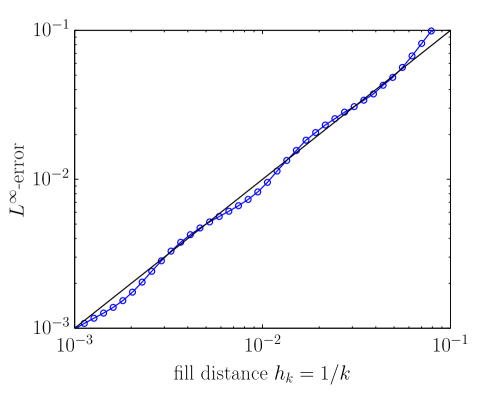
We begin with the simple one-dimensional system
on , with parameter and cost function Apparently, the optimal feedback is , yielding the optimal value function . We choose equidistant sets of nodes, , and use the Wendland function as shape function with parameter . In Figure 1, we show the -error of the approximate value function in dependence on the fill distance of the set of nodes . As predicted by Theorem 3, we observe a linear decay of the error in .
5.2. Example: shortest path with obstacles
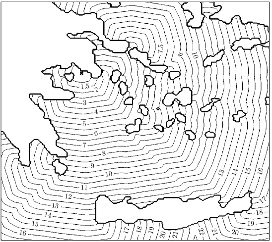
Our next example is supposed to demonstrate that state space constraints can trivially be dealt with, even if they are very irregular: We consider a boat in the mediteranian sea surrounding Greece (cf. Fig. 2) which moves with constant speed . The boat is supposed to reach the harbour of Athens in shortest time. Accordingly, the dynamics is simply given by
where we choose the time step , with , and the associated cost function by In other words, we are solving a shortest path problem on a domain with obstacles with complicated shape.
In order to solve this problem by our approach, we choose the set of nodes as those nodes of an equidistant grid which are placed in the mediteranean sea within the rectangle shown in Fig. (2), which we normalize to . We extracted this region from a pixmap of this region with resolution 275 by 257 pixels. The resulting set consisted of nodes. We choose . The position of Athens in our case is approximately given by and we choose . We again use the Wendland function as shape function with parameter .
In Figure (2), we show some isolines of the approximate optimal value function. The computation took around 10 seconds on our GHz Intel Core i5.
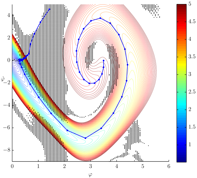
5.3. Example: an inverted pendulum on a cart
Our next example is two-dimensional as well, with only box constraints on the states, but the stabilization task is more challenging: We consider balancing a planar inverted pendulum on a cart that moves under an applied horizontal force, cf. [18] and Figure 3.
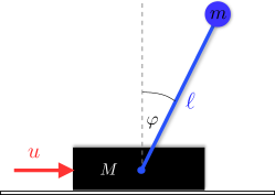
The configuration of the pendulum is given by the offset angle from the vertical up position and we do not consider the motion of the cart. Correspondingly, the state of the system is . The equation of motion becomes
| (8) |
where is the mass of the cart, the mass of the pendulum and is the distance of the center of mass from the pivot. We use for the mass ratio and for the gravitational constant. The stabilization of the pendulum is subject to the cost . For our computations, we need to obtain a discrete-time control system. To this end, we consider the time sampled system with sampling period and keep the control constant during the sampling period. In the computations, we used and computed the time sampling map via one explicit Euler step. As in [18], we choose as the region of interest and the set of nodes by a tensor product grid, using equally spaced points in each coordinate direction (cf. the Matlab code in the next section), and . We again use the Wendland function as shape function, the shape parameter is chosen such that the support of each overlaps with the supports of roughly other ’s, i.e. here.
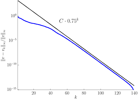
In Figure 4, we show the behavior of the (relative) -approximation error during the value iteration. We observe geometric convergence as expected by Theorem 2. The computation of the optimal value function took 6.8 seconds.
In Figure 5, some isolines of the approximate value function are shown, together with the complement of the set (cf. Proposition 1) as well as the first 80 points of a trajectory of the closed loop system with the optimal feedback. At the 30th iteration, the trajectory leaves the set and subsequently moves away from the target.
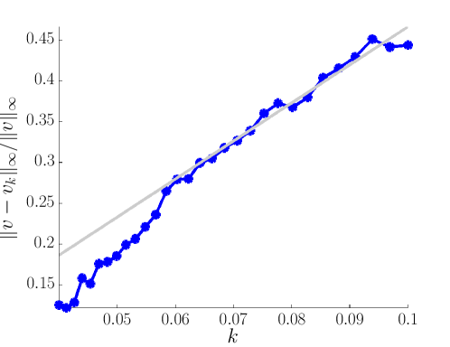
In Figure 6, the behavior of the error of the approximate optimal value function in dependence of the fill distance is shown. Here, we used the value function with fill distance as an approximation to the true one. Again, the convergence behavior is consistent with Theorem 3 which predicts a linear decay of the error. The corresponding Matlab code is given in Code 1.
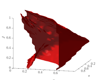
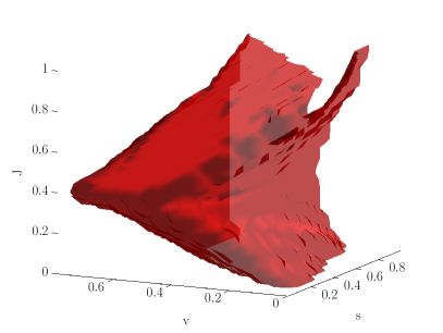
5.4. Example: magnetic wheel
We finally turn to an example with a three dimensional state space, the stabilization of a magnetic wheel, used in magnetic levitation trains, cf. [13] and Figure 7.

A point in state space is given by the gap between the magnet and the track, its change rate and the electrical current through the magnet. The input is the voltage applied to the circuit. The dynamics is given by
where , the target gap , the inductance of the magnet, the magnet mass , the ratio of the total mass and the magnet mass , the resistance , the leakage inductance and the gravitational constant . We consider the cost function
| (9) |
The model has an unstable equilibrium at approximately , which, again, we would like to stabilize by an optimal feedback. We choose as state space, as the set of controls, an equidistant grid of nodes in , the Wendland function as shape function with shape parameter , such that the support of each overlaps with the supports of roughly other ’s. The computation of the value function takes around 60 seconds. In figure 8 we show a subset of the stabilizable subset of , i.e. we show the set .
6. Future directions
There are many ways in which the approach from this paper can be extended. For example, it is natural not to fix the shape parameter at the same value for all basis functions . One could, e.g., either try to choose (greedily) in an optimal way for each or to implement a multilevel type scheme which works with a scale of values for . This also raises the issue of an improved or even optimal choice for the set of nodes (instead of the equidistant grid used here). One drawback of the value iteration used here is that the images of all possible node/control value pairs have to be computed and the corresponding matrix entries have to be stored. It would be nice to have some sort of “fast marching” type algorithm which needs this reachability information only locally. Finally, the approximation space that we use here is rather smooth – in contrast to the value function which in general is only Lipschitz-continuous. If one considers a relaxed version of the optimality principle, e.g. in the sense of [21], smoother solutions might exist which can be approximated with higher efficiency.
Appendix A Lipschitz continuity of
We assume that a discrete time control problem is given that is stabilizable on all of , i.e. that . Furthermore, we require that , , that is Lipschitz continuous w.r.t. with Lipschitz constant and is Lipschitz continuous w.r.t. resp. with Lipschitz constants and , resp., and that there is a feedback so that the closed-loop system has 0 as an asymptotically stable fixed point.
The idea of the proof of Lipschitz continuity of is that the number of time steps needed to steer an arbitrary starting point into a neighborhood of the equilibrium point is bounded. So the proof will consist of two parts, namely
-
(1)
finding a neighborhood of the equilibrium point where is Lipschitz continuous and
-
(2)
using the Lipschitz constants of and and the previously mentioned bound on the number of steps needed to control arbitrary initial points into the neighborhood of the equilibrium point and extending the proof of Lipschitz continuity from the neighborhood to the whole state space.
A.1. Local Lipschitz continuity
In the following, we will consider the approximation by the following LQR system:
where
Its optimal feedback is given by a linear map , where is a matrix, see [24]. The optimal feedback for the LQR system is not an optimal feedback for the original system, but a locally stabilizing one; let be the derived (not optimal) value function of this feedback for the original system. Consider the matrix-valued map
One has for the spectral radius because the original system has 0 as an asymptotically stable fixed point. So there is a norm on and an with . Choose open neighborhoods , s.t.
| (10) |
for .
We choose even smaller open sets by further requiring to be a sublevel set relative to , for all and for all .
Lemma 4.
Let . Then
is a pseudo-contraction relative to .
We use the expression pseudo-contraction to indicate that does not map to itself.
Proof.
By setting one gets the following corollary. Noting that is a sublevel set relative to , this time the map has images in .
Corollary 1.
is a contraction on relative to .
Corollary 2.
is continuous on , even Lipschitz continuous.
Proof.
was assumed to be Lipschitz continuous w.r.t. resp. with Lipschitz constant resp. . By equivalence of norms, is also Lipschitz continuous w.r.t. resp. with Lipschitz constants and relative to . Consequently, is Lipschitz continuous with Lipschitz constant relative to .
It follows from Lemma 4 that is Lipschitz continuous with Lipschitz constant relative to . This is seen by considering two points and comparing their trajectories under the feedback . Their mutual distances relative to develop at most like a geometric sequence with factor .
∎
Now we choose an open neighborhood according to the following lemma.
Lemma 5.
There is a neighborhood s.t. each optimal feedback (of the original system) on lies in .
Proof.
Because of compactness of and for , one has
One can choose s.t. , consequently
Now, for points in , the optimal controls are in . ∎
As an additional condition we require from that . So the Hausdorff distance is positive. We choose a neighborhood s.t. optimal trajectories starting in stay in . This is the case if . The last term is positive because of compactness of .
Lemma 6.
There is a neighborhood of where is Lipschitz continuous.
Proof.
For given with we choose as a nearly optimal control sequence for : and such that stays in . This is possible because is open. This gives us a sequence . For we define iteratively with
i.e. a “linear correction” with the information we have from the LQR system.
Consequently,
and thus
Changing the roles of and , and noting that two norms like and on a finite-dimensional space are equivalent, we conclude
for some . Choose with ∎
A.2. Global Lipschitz continuity
Lemma 7.
is bounded on .
Proof.
Let . Take a stabilizing control sequence . So there is an such that . Because of continuity of the system there is a neighborhood such that each is steered to in steps. On we already know that is bounded since on , so it is also bounded on because is bounded. Now by compactness of , finitely many such sets cover . So is also bounded on . ∎
Let . We assume to be bounded from below by outside of . Let be an integer with and . The definition of is such that each optimal trajectory reaches in at most steps.
From now on, let be the (an) optimal feedback which exists on because is continuous and so the right hand side of the Bellman equation depends continuously on .
Lemma 8.
Let . Then there is a neighborhood and a constant s.t. for any we have the following: Let an almost optimal control sequence for (but not for ) in the sense that it steers in at most steps to and Then
Proof.
Again, we consider trajectories of starting at with and control sequences resp. . Note that only is an almost optimal trajectory. By optimality of and the definition of , one has .
In addition, one has , so . Now,
∎
Theorem 4.
Let be the cost function of a discrete time control problem that is stabilizable on the compact state space , where the dynamical system is in , the cost function is in , and that has a feedback whose closed-loop system has 0 as an asymptotically stable fixed point. Then is Lipschitz continuous.
Proof.
From the setting in the proof of the preceding lemma and by choosing appropriately, we get
Changing the roles of and , we conclude
Now, of course, we can skip the assumption , because a local everywhere Lipschitz constant is also a global Lipschitz constant. ∎
By the definition of as , the function is also Lipschitz continuous, say with Lipschitz constant . In general, and can not be expected to be differentiable.
References
- [1] H. Alwardi, S. Wang, L. Jennings, and S. Richardson. An adaptive least-squares collocation radial basis function method for the hjb equation. J. Glob. Opt., 52(2):305–322, 2012.
- [2] M. Bardi and I. Capuzzo-Dolcetta. Optimal control and viscosity solutions of Hamilton-Jacobi-Bellman equations. Birkhäuser, Boston, Boston, MA, 1997.
- [3] R. Bellman. Dynamic programming. Princeton University Press, Princeton, NJ, 1957.
- [4] D. Bertsekas. Dynamic programming. Prentice Hall Inc., Englewood Cliffs, NJ, 1987.
- [5] I. Capuzzo-Dolcetta. On a discrete approximation of the Hamilton-Jacobi equation of dynamic programming. Appl. Math. Optim., 10(1):367–377, 1983.
- [6] I. Capuzzo-Dolcetta and M. Falcone. Discrete dynamic programming and viscosity solutions of the Bellman equation. Ann. Inst. H. Poincaré Anal. Non Linéaire, 6(suppl.):161–183, 1989.
- [7] E. Carlini, M. Falcone, and R. Ferretti. An efficient algorithm for Hamilton-Jacobi equations in high dimension. Comput. Vis. Sci., 7(1):15–29, 2004.
- [8] T. Cecil, J. Qian, and S. Osher. Numerical methods for high dimensional Hamilton-Jacobi equations using radial basis functions. J. Comp. Phys., 196(1):327 – 347, 2004.
- [9] M. Falcone. A numerical approach to the infinite horizon problem of deterministic control theory. Appl. Math. Optim., 15(1):1–13, 1987.
- [10] M. Falcone and R. Ferretti. Discrete time high-order schemes for viscosity solutions of Hamilton-Jacobi-Bellman equations. Numer. Math., 67(3):315–344, 1994.
- [11] M. Falcone and R. Ferretti. High-order approximations for viscosity solutions of Hamilton-Jacobi-Bellman equations. In Nonlinear variational problems and partial differential equations (Isola d’Elba, 1990), volume 320 of Pitman Res. Notes Math. Ser., pages 197–209. Longman Sci. Tech., Harlow, 1995.
- [12] G. Fasshauer. Meshfree Approximation Methods with Matlab. World Scientific, 2007.
- [13] E. Gottzein, R. Meisinger, and L. Miller. Anwendung des ”Magnetischen Rades” in Hochgeschwindigkeitsmagnetschwebebahnen. ZEV-Glasers Annalen, 103, 1979.
- [14] L. Grüne. An adaptive grid scheme for the discrete Hamilton-Jacobi-Bellman equation. Numer. Math., 75(3):319–337, 1997.
- [15] L. Grüne. Error estimation and adaptive discretization for the discrete stochastic Hamilton-Jacobi-Bellman equation. Numer. Math., 99(1):85–112, 2004.
- [16] L. Grüne and O. Junge. A set oriented approach to optimal feedback stabilization. Syst. Cont. Lett., 54(2):169–180, Feb. 2005.
- [17] C. Huang, S. Wang, C. Chen, and Z. Li. A radial basis collocation method for Hamilton-Jacobi-Bellman equations. Automatica, 42(12):2201–2207, 2006.
- [18] O. Junge and H. M. Osinga. A set oriented approach to global optimal control. ESAIM Control Optim. Calc. Var., 10(2):259–270, 2004.
- [19] C.-Y. Kao, S. Osher, and Y.-H. Tsai. Fast sweeping methods for static Hamilton-Jacobi equations. SIAM J. Numer. Anal., 42(6):2612–2632, 2005.
- [20] S. N. Kružkov. Generalized solutions of Hamilton-Jacobi equations of eikonal type. I. Mat. Sb. (N.S.), 98(140):450–493, 1975.
- [21] B. Lincoln and A. Rantzer. Relaxing dynamic programming. IEEE Trans. Auto. Ctrl., 51(8):1249 –1260, 2006.
- [22] W. McEneaney. Max-plus methods for nonlinear control and estimation. Birkhäuser, Boston, 2006.
- [23] J. A. Sethian and A. Vladimirsky. Ordered upwind methods for static Hamilton-Jacobi equations: theory and algorithms. SIAM J. Numer. Anal., 41(1):325–363, 2003.
- [24] E. Sontag. Mathematical Control Theory: Deterministic Finite Dimensional Systems. Springer, 1998.
- [25] H. Wendland. Piecewise polynomial, positive definite and compactly supported radial functions of minimal degree. Adv. Comp. Math., 4:389–396, 1995.