Afterglows from precursors in Gamma Ray Bursts. Application to the optical afterglow of GRB 091024

Abstract

About 15% of Gamma Ray Bursts have precursors, i.e. emission episodes preceding the main event, whose spectral and temporal properties are similar to the main emission. We propose that precursors have their own fireball, producing afterglow emission due to the dissipation of the kinetic energy via external shock. In the time lapse between the precursor and the main event, we assume that the central engine is not completely turned off, but it continues to eject relativistic material at a smaller rate, whose emission is below the background level. The precursor fireball generates a first afterglow by the interaction with the external circumburst medium. Matter injected by the central engine during the ”quasi-quiescent” phase replenishes the external medium with material in relativistic motion. The fireball corresponding to the main prompt emission episode rams into this moving material, producing a second afterglow, and finally catches up and merges with the first precursor fireball. We test this scenario over GRB 091024, an event with a precursor in the prompt light curve and two well defined bumps in the optical afterglow, obtaining an excellent agreement with the existing data.

1 Introduction

Around 15% of Gamma Ray Bursts (GRBs), show precursors in the light curve of their prompt emission. Despite its definition is somewhat subjective, a “precursor” can be identified as emission (i) preceding main event, with a maximum flux (or count rate) which is less than the main event, and (ii) separated from the latter by a time interval in which the flux is at the background level (for different definitions of precursors and different ways to find GRBs with precursors see Koshut et al. 1995, Lazzati 2005, Burlon et al. 2008, 2009).

The main question still to be addressed is whether precursors have a different origin than the main event in GRBs or not. This issue has been explored observationally by comparing the energetics and spectra of precursors with those of the main event and more in general with those of GRBs without precursors (e.g. Burlon et al. 2008, 2009). The spectrum and variability timescale of precursors are similar to those of the main event. On average, precursors have a fluence (flux integrated over its duration) about one tenth of that of their associated main events. Also the time evolution of the spectrum of precursors is consistent with that of GRBs without precursors (Burlon et al. 2009). These facts strongly suggest that the precursors are not a separated emission component, produced by something different from the central engine responsible for the main event. They are simply the first phases of the central engine activity.

The key question is then why the central engine can have periods of time in which it is quiescent even for over 100 s in the rest frame of the source. Some GRBs showed more than one precursors, and precursors have been seen also in short bursts (a typical example is GRB 090510, a very bright short GRB observed also above 100 MeV by the Large Area Telescope onboard the Fermi satellite, see Ackermann et al. 2010; for other examples see Troja, Rosswog & Gehrels 2010).

The explanation of the precursor phenomenon remains a puzzle. The fact that there can be more than one precursor in one GRB rules out the “two step engine” model (see e.g. Wang & Mészáros 2007; Lipunova et al. 2009) in which the precursor corresponds to the formation of a compact object that after a while collapses into a black hole, originating the main GRB event. The fact that the spectrum is not a blackbody (Lazzati et al. 2005; Burlon et al. 2008, 2009) and that the quiescent times are often very long rule out the fireball precursor models (see e.g. Mészáros & Rees 2000; Ruffini et al. 2001; Daigne & Mochkovitch 2002; Lyutikov & Blandford 2003; Li 2007) that associate the precursor emission to the thermal radiation initially trapped in the fireball. Analogously, the non–thermal nature of the precursor’s spectrum rules out the “progenitor precursor” models (Ramirez–Ruiz et al. 2002; Lazzati & Begelman 2005) based on the collapsar scenario, in which the precursor corresponds to the interaction of a weakly relativistic jet with the stellar envelope.

Recently, Bernardini et al. (2013, 2014) put forward a new model able to explain the presence of one or more precursors with non–thermal emission. They assume that the central powerhouse is a newly born accreting magnetar; in this model accretion can be halted by the centrifugal drag exerted by the rotating magnetosphere onto the infalling matter, allowing for multiple precursors and very long quiescent times.

So far, however, precursors have been studied only in relation to the fact that they are observed in the high energy prompt light curve of GRBs. Here we consider the possibility that some features of the afterglow emission can be ascribed to the precursor activity. In a nutshell, since the energy emitted by precursors is a large fraction (10–50%) of the total energy of the bursts, we can assume that precursors originate fireballs as well as it is thought for the main event, and that these fireballs run into the circumburst medium (CBM).

Therefore, precursors should produce an external shock, namely, an afterglow, similarly to what is thought to happen for the main emission episode of any GRB. When the quiescent time between the precursors and the main event is sufficiently long, as in the case of GRB 060124 (Romano et al. 2006) and GRB 050820A (Cenko et al. 2006), we have the opportunity to see this afterglow emission (in between the precursor and the main event episodes).

The precursor fireball, being the first to interact with the CBM, will “sweep” it and set it in motion with a certain velocity. Then the central engine enters a phase of quiescence, ejecting matter at a much reduced rate, whose emission remains below the background level. This matter fills the circumburst region. When the central engine becomes active again, producing the main event of the prompt emission, a new fireball is produced, running into the moving CBM ejected during the quiescence phase. The corresponding shock is weaker than the shock into a stationary CBM, since the relative kinetic energy between the shock and the moving CBM is less than in the case of an unperturbed and stationary CBM. The main event fireball would then decelerate less, and it will catch up with the first fireball, shock it, and merge.

We apply these ideas to a specific burst, GRB 091024 (Gruber et al. 2011; Virgili et al. 2013), a very long burst ($T_{\rm 90}=1024$ s) with a precursor lasting $\sim 70$ seconds, a quiescent time of $\sim 600$ seconds, a second precursor lasting $\sim 40$ s, another quiescent time of $\sim 170$ seconds, and a complex main event, lasting $\sim 200$ seconds with pronounced variability.

The long duration and quiescent time allowed to have a dense optical coverage of the light–curve, especially during the quiescent time (Virgili et al. 2013). Its properties make GRB 091024 an ideal test case for our new scenario, and we anticipate that the results are very encouraging.

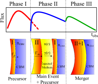
Figure 1: Cartoon of the proposed scenario. On the top we show the three phases of the afterglow emission, that correspond to the three configurations illustrated in the bottom: Phase 1): Fireball I (associated to the precursor) runs into the circumburst medium originating the first afterglow. Phase 2): Fireball II (associated to the main event) runs into the moving material ejected by the central engine during the quiescent phase, producing the second peak of the afterglow light curve. Phase III: Fireballs I and II merge, producing a brightening of the afterglow.

In §2 we describe the main features of the proposed scenario, we detail its dynamical and radiative evolution in §2.2, 2.3, 2.4. The model is then applied to the optical light curve of GRB 091024 in §3 and §4. We draw our conclusions in §4.

2 Proposed scenario

Burlon et al. (2008) showed that precursors have spectral and temporal properties similar to the main event emission, so it is reasonable to think that the same central engine is responsible for both. Fig. 1 shows a cartoon of the proposed scenario, whose main features can be summarized as follows:

• The precursor, being nothing else that the first pulse of the prompt emission, produces its own fireball (called “fireball I” hereafter) that shocks the circumburst material (with density $n_{\rm CBM}$) producing an afterglow emission (the peak is shown by the solid red line in the top panel of Fig.1).

• During the “quiescent” phase of apparent no emission, the central engine is not completely switched off, but it continues to eject relativistic matter, albeit at a much reduced rate. At the end of this quiescent phase, the central engine fully reactivates, producing the main prompt event associated to “fireball II”.

• Fireball II can interact with this continuously ejected material and produce a second afterglow emission. The shock will be less efficient than the first one because it is produced in a medium that is moving. This explains the presence of a second peak in the optical light curve, in this case associated with the second emitted fireball, i.e. that of the main event.

• For simplicity, the density and the bulk Lorentz factor profile of the ejected medium are assumed to be power–laws:

  $$\begin{matrix}n(R)=n_{0}(R/R_{0})^{-s}\\ \gamma(R)=\gamma_{0}(R/R_{0})^{-g}\end{matrix}$$ (1)

• If fireball I decelerates more than fireball II, by the interaction with the external medium, a merger between the two fireball occurs. During the merger some energy is released (with a mechanism that is similar to internal shocks) and a merged fireball (I+II) is formed. This fireball decelerates in the external medium generating the last part of the afterglow emission. This episode can be seen as an injection of new kinetic energy from the fireball II to the decelerating fireball I (refreshed shock, Rees & Mészáros 1998). This produces a rebrightening episode.

Summarizing, we identify three distinct afterglow emission phases:

1. The first afterglow produced by the deceleration of fireball I in the CBM.

2. The second afterglow produced by the deceleration of fireball II in the medium ejected by the central engine, albeit at a reduced rate;

3. The last part of the afterglow produced by the merged fireballs (I+II) interaction with the external medium.

For each of these three portions we need to study the dynamical behaviour of the fireball and how the dissipated energy is converted into radiation.

2.1 Dynamics

This work requires a non–standard dynamical treatment because the afterglow is produced by the interaction of a relativistic fireball with a medium that is moving with respect to the central engine. We propose a new approach, inspired by Nava et al. (2013), based on the energy–momentum conservation in the collision of the fireball with the external CBM, that can be in motion or at rest. Here we consider the case of an external medium that is moving with a Lorentz factor profile $\gamma(R)$. We assume that the fireball has initial mass $M_{0}$ and initial Lorentz factor $\Gamma_{0}$. In the collision with the external CBM, the fireball collects the mass of the encountered CBM and when the collected mass is large enough, the fireball starts to decelerate, reducing its bulk Lorentz factor $\Gamma(R)$.

In the collision, some bulk kinetic energy is transformed into internal energy $\varepsilon^{\prime}$ (as measured in the fireball comoving frame). A fraction of this internal energy (labeled as $\varepsilon^{\prime}_{\rm RAD}$) is radiated and no longer contributes to the inertia of the fireball; the amount of radiated energy depends on the specific radiative process and it will be analysed in the following section.

If $\varepsilon^{\prime}_{\rm RAD}\ll\varepsilon^{\prime}$, the fireball is a very inefficient radiator, so the radiative losses are negligible and the dynamical evolution of the fireball can be described separately by the radiative emission behaviour. Since the total fireball energy is conserved, this case is called adiabatic regime.

In the opposite case, if $\varepsilon^{\prime}_{\rm RAD}\sim\varepsilon^{\prime}$, almost all the internal energy is lost in radiation. Also in this case the fireball dynamical evolution can be treated separately by the radiative emission, and it is called radiative regime.

In the intermediate case, the dynamical evolution is strictly linked to the radiative behaviour, so both aspects have to be considered simultaneously.

To describe the dynamical evolution of the fireball and to compute the amount of dissipated energy we solved numerically the equations of the energy–momentum conservation step–by–step. At radius $R$, the fireball with Lorentz bulk factor $\Gamma(R)$ and mass $M(R)$ hits an element of external medium $\Delta m=4\pi R^{2}n(R)m_{p}\Delta R$ that is moving with a Lorentz factor $\gamma(R)$; from energy–momentum conservation, we can obtain the value of the dissipated energy in the collision $\Delta\varepsilon^{\prime}(R)$ and the new Lorentz factor $\Gamma(R+\Delta R)$.

A fraction $\epsilon_{e}$ of the dissipated energy is given to the CBM electrons, that can emit a part of it as radiation. We assume that we can write the radiated energy $\Delta\varepsilon^{\prime}_{\rm RAD}$ as:

$$\Delta\varepsilon^{\prime}_{\rm RAD}(R)=\zeta(R)\epsilon_{e}\Delta\varepsilon^{\prime}(R)$$ (2)

where $\zeta(R)$ is the fraction of electron energy that is radiated at $R$ (this value depends on the radiative process and it will be calculated in §2.3). We obtain the comoving emitted bolometric luminosity:

$$L^{\prime}_{\rm bol}=\frac{\Delta\varepsilon^{\prime}_{\rm RAD}}{\Delta t^{\prime}}=\frac{\Delta\varepsilon^{\prime}_{\rm RAD}}{\Delta R}\frac{\Delta R}{\Delta t_{\perp}}\frac{\Delta t_{\perp}}{\Delta t^{\prime}}=\Gamma\beta c\frac{\Delta\varepsilon^{\prime}_{\rm RAD}}{\Delta R}$$ (3)

where $\Delta t_{\perp}=\Delta R/(\beta c)$ is the time interval corresponding to the distance $\Delta R$ measured by an observer placed perpendicularly to the burst direction, $\Delta t^{\prime}$ is the same time measured by a comoving observer, $\beta$ is the bulk velocity of the fireball (in unit of $c$) and $\Gamma$ is the bulk Lorentz factor of the fireball.

2.2 Times

The time interval $\Delta t_{\rm obs}$ corresponding to the distance $\Delta R$ measured by an observer placed close to the axis of the burst can be written as:

$$\Delta t_{\rm obs}=(1+z)\frac{1-\beta\cos\theta}{\beta c}\Delta R$$ (4)

where $z$ is the cosmological redshift and $\theta$ is the angle between the line of sight and the burst axis.

The observed bolometric luminosity observed at time $t_{\rm obs}$ is constituted by the photons arriving to the detector at the time $t_{\rm obs}$, but that have been emitted at different times. The real emitting surface seen at time $t_{\rm obs}$ is called equal arrival time surface and it is non–trivial to determine.

We approximate the determination of the equal arrival time surfaces by considering that most of the received emission comes from the ring of aperture angle $\sin\theta=1/\Gamma$ (or equivalently $\cos\theta=\beta$). In this way Eq. 4 simplifies in

$$\Delta t_{\rm obs}=(1+z)\frac{\Delta R}{\beta c\Gamma^{2}}$$ (5)

The observed bolometric luminosity can be written as:

$$L_{\rm bol}=\delta^{2}L^{\prime}_{\rm bol}$$ (6)

where $\delta=\left[\Gamma(1-\beta\cos\theta)\right]^{-1}$ (equal to $\Gamma$ for $\cos\theta=\beta$) is the relativistic Doppler factor (or beaming factor). The obtained bolometric luminosity is a function of time, so we will label it with $L_{\rm bol}(t)$.

2.3 Radiative emission

In this section we calculate the synchrotron emission observed at the frequency $\nu=\nu_{\rm obs}(1+z)$. We propose a new method based on the normalization of the synchrotron spectrum to the bolometric luminosity computed in the previous sections. Most of the equations used in this section are inspired by the work of Panaitescu & Kumar (2000), generalizing them in order to describe the emission produced by the interaction with a medium that has been pre–accelerated to relativistic speed.

We explicitly apply an energy conservation equation, by requiring that in the fast cooling regime the frequency integrated spectrum is equal to the power that the shock gives to the electrons, as measured in the observer frame:

$$\int L_{\nu}(t)\mbox{d}\nu=\Gamma^{2}\epsilon_{\rm e}{\Delta\varepsilon^{\prime}\over\Delta t^{\prime}}$$ (7)

We assume that the synchrotron emission is produced by a distribution of electrons that is the result of a continuous particle injection and the cooling due to the emission. We label with $Q(\gamma)$ the number of injected electrons with energy $\gamma m_{e}c^{2}$ for unity of time and volume, $N(\gamma)$ the energetic distribution for unity of volume and $\dot{\gamma}$ the cooling rate. They are linked by the continuity equation:

$$\frac{\partial N(\gamma)}{\partial t}=\frac{\partial}{\partial\gamma}\left[\dot{\gamma}N(\gamma)\right]+Q(\gamma)$$ (8)

For a stationary source $\partial N\left(\gamma\right)/\partial t=0$.
We assume that the injection distribution is a power law of index $2<p<3$:

$$Q(\gamma)\propto\gamma^{-p}\mbox{ for }\gamma_{i}<\gamma<\gamma_{\rm max},$$ (9)

where $\gamma_{i}$ is called injection energy.

The synchrotron cooling rate is:

$$\dot{\gamma}_{\rm syn}m_{\rm e}c^{2}=\frac{4}{3}\sigma_{\rm T}cU_{B}\gamma^{2}$$ (10)

The synchrotron cooling time is (Sari et al., 1998):

$$t_{\rm c,syn}=\frac{\gamma}{\dot{\gamma}_{syn}}=\frac{3m_{\rm e}c}{4\sigma_{\rm T}U_{B}\gamma}$$ (11)

For each time, we define the cooling energy $\gamma_{c}(t)m_{\rm e}c^{2}$, that is the energy that an electron must have so that its cooling time is equal to the scale time of expansion of the fireball. Under these conditions we have two possible solutions of Eq. 8 (see also Sari & Esin, 2001):

• Fast Cooling regime: $\gamma_{\rm c}<\gamma_{\rm i}$. In this case all injected electrons cool in a time shorter than the dynamical time (time needed to double the fireball radius). The corresponding energy distribution $N_{\rm FC}(\gamma)$ is

  $$N_{\rm FC}(\gamma)=\begin{cases}0&\gamma<\gamma_{\rm c},\\ N_{\rm i}\left(\frac{\gamma}{\gamma_{\rm i}}\right)^{-2}&\gamma_{\rm c}<\gamma<\gamma_{\rm i},\\ N_{\rm i}\left(\frac{\gamma}{\gamma_{\rm i}}\right)^{-(p+1)}&\gamma_{\rm i}<\gamma<\gamma_{\rm max}\\ \end{cases}$$ (12)

• Slow Cooling regime: $\gamma_{\rm i}<\gamma_{\rm c}$. In this case a fraction of (or all) the injected electrons do not cool in a dynamical time. The corresponding energy distribution $N_{\rm SC}(\gamma)$ is

  $$N_{\rm SC}(\gamma)=\begin{cases}0&\gamma<\gamma_{\rm i},\\ N_{\rm c}\left(\frac{\gamma}{\gamma_{\rm c}}\right)^{-p}&\gamma_{\rm i}<\gamma<\gamma_{\rm c},\\ N_{\rm c}\left(\frac{\gamma}{\gamma_{\rm c}}\right)^{-(p+1)}&\gamma_{\rm c}<\gamma<\gamma_{\rm max}\\ \end{cases}$$ (13)

  In this work we will not derive the normalizations $N_{\rm i}$ and $N_{\rm c}$ of the electrons energy distribution, but we will compute directly the normalizations of the emitted synchrotron spectrum (see §2.3.3).

2.3.1 Break frequencies

Generalizing Panaitescu & Kumar (2000) in the case of a pre–accelerated medium we have the following relations:

$$\gamma_{\rm i}=\epsilon_{e}\,{m_{\rm p}\over m_{\rm e}}\,{p-2\over p-1}\,(\Gamma_{\rm rel}-1)$$ (14)

$$\gamma_{c}=\frac{15\pi}{1+y}\,\frac{m_{\rm e}c^{2}\Gamma}{\sigma_{\rm T}B^{2}R}$$ (15)

$$U_{B}=\frac{B^{2}}{8\pi}=\epsilon_{B}n(R)m_{p}c^{2}(\Gamma_{\rm rel}-1)(4\Gamma_{\rm rel}+3)$$ (16)

$$y=\frac{4}{3}\tau_{\rm e}\left\langle\gamma^{2}\right\rangle$$ (17)

$$\tau_{e}=\frac{1}{4\pi}\frac{\sigma_{\rm T}m(r)}{m_{\rm p}R^{2}}$$ (18)

where $U_{B}$ is the magnetic energy density, $y$ is the Comptonization parameter, $\tau_{\rm e}$ is the electron optical depth, $\left\langle\gamma^{2}\right\rangle$ is the average of the square of the random electron Lorentz factor, $\Gamma_{\rm rel}$ is the relative Lorentz factor between the fireball and the external medium, as measured in one of the two frames, and $\epsilon_{\rm e}$, $\epsilon_{B}$ are the fractions of the dissipated internal energy that are given respectively to leptons and to the magnetic field. The injection and the cooling frequency are:

$$\nu_{\rm i}=\frac{4}{3}\frac{eB}{2\pi m_{\rm e}c}\Gamma\gamma_{\rm i}^{2}$$ (19)

$$\nu_{\rm c}=\frac{4}{3}\frac{eB}{2\pi m_{\rm e}c}\Gamma\gamma_{c}^{2}$$ (20)

For simplicity, we will not consider the self–absorbed part of the spectrum when calculating the normalization, since it is less relevant for the total energy. Anyway we will compute the self–absorption frequency $\nu_{\rm a}$ using Eq. 52 in Panaitescu & Kumar (2000). The equation used is:

$$\nu_{\rm a}=\nu_{\rm m}\left(\frac{3-s}{5}\frac{B\gamma_{\rm m}^{5}}{enR}\right)^{-\alpha}\mbox{,}\quad\alpha=\begin{cases}-\frac{3}{5}&\nu_{\rm a}<\nu_{\rm m}\\ -\frac{2}{q+4}&\nu_{\rm a}>\nu_{\rm m}\\ \end{cases}$$ (21)

where $\nu_{\rm m}=\min(\nu_{\rm i},\nu_{\rm c})$, $\gamma_{\rm m}=\min(\gamma_{\rm i},\gamma_{\rm c})$ and $q=2$ in fast cooling regime $(\nu_{\rm c}<\nu_{\rm i})$ or $q=p$ in slow cooling regime $(\nu_{\rm i}<\nu_{\rm c})$.

The fraction of emitted energy $\zeta$ (cfr. Eq. 2) can be expressed as the ratio between the power emitted in slow cooling regime and in fast cooling regime.

$$\zeta=\frac{\left[\int N(\gamma)\dot{\gamma}\mbox{d}\gamma\right]_{\rm SC}}{\left[\int N(\gamma)\dot{\gamma}\mbox{d}\gamma\right]_{\rm FC}}=\begin{cases}\frac{\gamma_{\rm i}}{\gamma_{\rm c}}\frac{p-2}{3-p}\left[\frac{1}{p-2}\left(\frac{\gamma_{c}}{\gamma_{\rm i}}\right)^{3-p}-1\right]&\gamma_{\rm i}\leq\gamma_{\rm c},\\ 1&\gamma_{\rm c}<\gamma_{\rm i}\\ \end{cases}$$ (22)

where we used $\dot{\gamma}=\dot{\gamma}_{\rm syn}$. Obviously, in the fast cooling regime we must have $\zeta=1$.

2.3.2 Comptonization parameter $y$

We introduce here a new way to estimate the Comptonizazion parameter $y$. The bolometric luminosity is constituted by two main components: the synchrotron emission and the SSC.

$$L^{\prime}_{\rm syn}+L^{\prime}_{\rm SSC}=L^{\prime}_{\rm bol}=\zeta(y)P^{\prime}_{\rm e}$$ (23)

where $P^{\prime}_{\rm e}$ is the total power distributed to the electrons, i.e. (cfr. Eq. 2):

$$P^{\prime}_{\rm e}=\epsilon_{\rm e}\frac{\Delta\varepsilon^{\prime}}{\Delta t^{\prime}}$$ (24)

$P^{\prime}_{\rm e}$ is obtained from purely dynamical considerations and does not depend on the particular emission mechanism chosen. We can express the synchrotron luminosity as (see Ghisellini et al. 2010):

$$L^{\prime}_{\rm syn}=\int 4\pi R^{2}\Delta R^{\prime}N(\gamma)\dot{\gamma}_{\rm syn}m_{\rm e}c^{2}\mbox{d}\gamma$$ (25)

Following Eq. 17 we have

$$y={4\over 3}\sigma_{\rm T}\Delta R^{\prime}\int N(\gamma)\gamma^{2}d\gamma$$ (26)

The we have:

$$L^{\prime}_{\rm syn}=4\pi R^{2}cU_{B}y$$ (27)

Dividing both sides for $4\pi R^{2}c$ we obtain the energy density of the synchrotron emission:

$$U_{\rm syn}=\frac{L^{\prime}_{\rm syn}}{4\pi R^{2}c}=yU_{B}$$ (28)

Adopting again Eq. 25 with $\dot{\gamma}_{\rm SSC}=(4/3)\sigma_{\rm T}c\gamma^{2}U_{\rm syn}/(m_{\rm e}c^{2})$ we can express the SSC luminosity as:

$$L^{\prime}_{\rm SSC}=4\pi R^{2}cU_{\rm syn}y=yL^{\prime}_{\rm syn}=y^{2}4\pi R^{2}cU_{B}$$ (29)

valid as long as the scattering is in the Thomson regime. Combining the Eqs. 23, 27 and 29 we obtain an important relation:

$$4\pi R^{2}cU_{B}(y+y^{2})=\zeta(y)P_{e}^{\prime}$$ (30)

We obtain the Comptonization parameter $y$ by numerically solving:

$$\frac{y+y^{2}}{\zeta(y)}=\frac{P^{\prime}_{\rm e}}{4\pi R^{2}cU_{B}}$$ (31)

2.3.3 Normalized synchrotron spectrum

The synchrotron spectrum can be written as Eq. 32 or Eq. 33, in the fast and slow cooling regime respectively (see also Sari et al, 1998, for the shape of the spectrum).

$$L_{\rm\nu,syn}^{FC}=A_{\rm FC}\begin{cases}\left(\frac{\nu}{\nu_{\rm c}}\right)^{1/3}&\nu<\nu_{\rm c}\\ \left(\frac{\nu}{\nu_{\rm c}}\right)^{-1/2}&\nu_{\rm c}<\nu<\nu_{\rm i}\\ \left(\frac{\nu}{\nu_{\rm i}}\right)^{-p/2}\left(\frac{\nu_{\rm c}}{\nu_{\rm i}}\right)^{1/2}&\nu_{\rm i}<\nu<\nu_{\rm max}\\ \end{cases}$$ (32)

$$L_{\rm\nu,syn}^{\rm SC}=A_{\rm SC}\begin{cases}\left(\frac{\nu}{\nu_{\rm i}}\right)^{1/3}&\nu<\nu_{\rm i}\\ \left(\frac{\nu}{\nu_{\rm i}}\right)^{-(p-1)/2}&\nu_{\rm i}<\nu<\nu_{\rm c}\\ \left(\frac{\nu}{\nu_{\rm c}}\right)^{-p/2}\left(\frac{\nu_{\rm i}}{\nu_{\rm c}}\right)^{(p-1)/2}&\nu_{\rm c}<\nu<\nu_{\rm max}\\ \end{cases}$$ (33)

where $A_{\rm FC}$ and $A_{\rm SC}$ are normalizing constants. In Eqs. 32 and 33, we neglected the self-absorbed part of spectrum, because we do not consider the evolution of the radio afterglow. We can obtain the normalizations imposing:

$$L_{\rm syn}+L_{\rm SSC}=L_{\rm syn}(1+y)=L_{\rm bol}$$ (34)

or

$$\int L_{\rm\nu,syn}\mbox{d}\nu=\frac{L_{\rm bol}}{1+y}=\zeta{\Gamma^{2}\epsilon_{\rm e}\over 1+y}{\Delta\epsilon^{\prime}\over\Delta t^{\prime}}$$ (35)

where $L_{\rm bol}$ is obtained from the dynamical energy–momentum conservation. Remembering that $\nu=\nu_{\rm obs}(1+z)$, the observed monochromatic flux can be written as:

$$F_{\nu_{\rm obs}}=\frac{\nu}{\nu_{\rm obs}}\frac{L_{\nu}}{4\pi d_{L}^{2}}=(1+z)\frac{L_{\nu}}{4\pi d_{L}^{2}}$$ (36)

where $d_{L}$ is the luminosity distance. Determining for each time the specific flux $F_{\nu_{\rm obs}}$, we obtain the monochromatic flux light curve, i.e. the function $F_{\nu_{\rm obs}}(t)$.

With the above approach we obtain the monochromatic synchrotron light curves of the GRB afterglow in a way that ensures the conservation of energy and momentum.

2.4 Model parameters and observables

We can divide the model parameters in the following six groups. Precursor parameters

• $\Gamma_{\rm 0,p}$: Initial Lorentz factor of the precursor fireball

• $E_{\rm k,p}$: Isotropic equivalent kinetic energy of the precursor fireball

• $T_{\rm p}$: Duration of the precursor emission

• $E_{\rm peak,p}$: Peak energy of the precursor

The last two quantities are measurable and the kinetic energy $E_{\rm k,p}$ can be obtained by the isotropic equivalent energy of the precursor $E_{\rm ISO,p}$ from the relation: $E_{\rm ISO,p}={\eta}E_{\rm k,p}$, where $\eta$ is the efficiency of conversion of the kinetic energy in radiative energy. We will assume $\eta\simeq 0.2$ (Frail et al., 2001 and see Ref. in Ghirlanda et al., 2004). The isotropic equivalent energy can be obtained from the observed fluence $\mathcal{F}$ with:

$$E_{\rm ISO}={4\pi d_{L}^{2}\over(1+z)}\mathcal{F}$$ (37)

So the only free parameter of the precursor is the initial Lorentz factor $\Gamma_{\rm 0,p}$.

Circumburst medium density parameters

The density profile of the external circumburst medium strongly influences the shape of the afterglow light curve. In the general case, the density profile can be written as:

$$n(R)=AR^{-s}$$

In the literature, two cases are usually considered: $s=0$ (homogeneous profile), $s=2$ (wind profile).

Following Sari (1997) and Ghisellini et al. (2010), the observed bolometric luminosity is:

$$L\propto\Gamma^{8}t^{2}n$$

with $R\propto t\Gamma^{2}$.

In the coasting phase $\Gamma$ is constant, implying $L\propto t^{2}n$ and $R\propto t$. If the medium is homogeneous, we then have $L\propto t^{2}$. Instead, for a wind medium, $L\propto t^{0}$ since the increase of the observable surface ($\propto R^{2}\propto t^{2}$) is compensated by the decreasing density ($n\propto R^{-2}\propto t^{-2}$).

The model is valid with both density profiles. When an initial rise of the early afterglow optical flux is observed, we will assume (in the following application of the model) that the precursor propagates in a homogeneous circumburst medium. In this case the density of the circumburst medium $n$ is another free parameter of the model.

Main event parameters

• $\Gamma_{\rm 0,m}$: Initial Lorentz factor of the main event fireball

• $E_{\rm k,m}$: Isotropic equivalent kinetic energy of the main event fireball

• $T_{\rm m}$: Duration of the main event emission

• $E_{\rm peak,m}$: Peak energy of the spectrum of the main event

• $\Delta t_{\rm main}$: Start time of the main event emission after the trigger

$\Delta t_{\rm main}$ can be directly observed. As in the previous case, the only free parameter is the initial Lorentz factor $\Gamma_{\rm 0,m}$.

Injected medium parameters

The matter injected by the central engine in the quasi–quiescence phases can be described with 4 parameters characterizing the density $n(R)$ and velocity $\gamma(R)$ profile, i.e. $\gamma_{0}$, $g$, $n_{0}$ and $s$ (see Eq. 1).

Merging parameters

These parameters describe the third phase of the afterglow light curve, after the merging of fireball I and II.

• $t_{\rm merg}$: Merging time of the two fireballs

• $\Gamma_{\rm merg}$: Initial Lorentz factor of the merged fireball

• $E_{\rm k,merg}$: Isotropic equivalent kinetic energy of the merged fireball

In this group there are no free parameters. The merging time $t_{\rm merg}$ can be determined studying the motion of the fireballs I and II that is completely determined from the parameters $\Gamma_{\rm p}(t)$, $\Gamma_{\rm m}(t)$, and the medium properties. $\Gamma_{\rm merg}$ and $E_{\rm k,merg}$ can be obtained from the equation of energy–momentum conservation during the merging.

Energy distribution parameters

For each part of the afterglow light curve, there are three free parameters:

• $\epsilon_{\rm e}$: Fraction of the internal energy given to electrons

• $\epsilon_{\rm B}$: Fraction of the internal energy given to magnetic field

• $p$: Injection spectral index of the electrons

Obviously we must have $\epsilon_{\rm e}+\epsilon_{\rm B}<1$.

The model has many free parameters (16, considering also the density $n$ of the circumburst medium), but they can be determined or limited by the observational data. The position of the peaks and the slopes in the light curves are the main observables that can constrain the parameters value. In particular we have: $(t_{\rm p},F_{\rm\nu,p})$ that are respectively the time and flux of the peak of the precursor afterglow, $(t_{\rm m},F_{\rm\nu,m})$ of the peak of the main event afterglow, $(t_{\rm merg},F_{\rm\nu,merg})$ that are the time and flux corresponding to the moment of the merger between fireball I and II.

From the slopes (especially for the second afterglow peak) we can infer the properties of the medium injected by the central engine (see also the application in §4.1 and Fig. 4).

2.5 Observable afterglow peaks and timescales

The three–peak afterglow scenario that we described should be the more common case, but other outcomes are possible. In fact, varying the time separation between precursor and main event fireballs, or modifying the properties of the injected medium we can reproduce different behaviours.

In the case at hands, the first peak in the afterglow light curve is interpreted as due to the deceleration of the precursor fireball in the external medium. The time of the onset of the precursor afterglow is strictly correlated with the deceleration time $t_{\rm dec}\propto(E_{\rm k}/n\Gamma_{0}^{8})^{1/3}$ (this relation is valid only for a homogeneous CBM; see Ghirlanda et al., 2012 and Nava et al., 2013 for more details). This requires that the fireball launched by the main event does not catch up the fireball of the precursor before the latter has decelerated. This can never happen if $t_{\rm dec}$ of the precursor fireball is shorter than the precursor–main event time interval. Instead, if the two fireballs interact before the deceleration time, the first afterglow peak disappears.

Knowing the density of the interstellar medium and the kinetic energy of the fireball, we can easily link the deceleration time to the initial bulk Lorentz factor. The presence of an optical peak between the precursor and the main event prompt emissions is key to constrain the value of the initial bulk Lorentz factor of the precursor. If the peak is not observed, we have $t_{\rm dec}(\Gamma_{0,\rm p})>\Delta t_{\rm main}$.

We cannot simply derive the deceleration time of the second fireball, since the main event propagates in a medium that is moving. This implies that it is difficult to constrain the initial bulk Lorentz factor of the main event, since its estimate depends on the properties of the injected medium.

The second peak is suppressed if the second fireball does not decelerate before reaching the first fireball. This occurs when the injected medium is moving too fast or has very low density.

3 Application to GRB 091024

As an application of our model, we study the broad band emission of GRB 091024, an extremely long GRB, with $T_{90}\sim 1,020$ s with precursor and a double peaked optical light curve. This burst is particularly suited to test our proposed model also because its optical light curve is highly sampled from 100 s to 1 day after the prompt emission. It was first detected by Fermi/GBM, that triggered at 08:55:58.47 UT ($t_{0}$) and again at 09:06:29.36 UT (Bissaldi & Connaughton, 2009). It was observed also by Konus–Wind (Golenetskii et al. 2009), and by Swift/BAT (Marshall et al., 2009), but the burst exited the BAT field of view at $t\sim 460$ s after the trigger and XRT measurements are available only $\sim 3,000$ s after the GBM trigger, because of Earth–limb constraints. The burst coordinates, according to XRT, are $\alpha_{J2000}=22^{h}37^{m}00.4$, $\delta_{J2000}=56^{\circ}53^{\prime}21^{\prime\prime}$, with an accuracy of 6 arcsec (Page & Marshall, 2009). Fermi/LAT was re–pointed at the burst direction, but it did not reveal any significant emission (Bouvier et al., 2009).

The acquisition of the first optical data started about a minute after the first trigger by the Super–LOTIS telescope (Updike et al., 2009). Other photometric data come from the Sonoita Research Observatory (SRO) and the Faulkes telescopes. The afterglow optical spectrum was obtained with the Low Resolution Imaging Spectrometer on telescope Keck I and by the spectrograph GMOS-N on Gemini North, measuring a cosmological redshift of $z=1.092$ (Cenko et al., 2009; Cucchiara et al., 2009).

The optical data that we use for the physical interpretation of the afterglow are published in Virgili et al. (2013).

3.1 Prompt emission

The analysis of the entire prompt emission can be found in Virgili et al. (2013) and Gruber et al. (2011); here we present only the main results of these analyses and we focus on the afterglow emission interpretation. The background subtracted light curve of prompt emission measured by Fermi/GBM is shown in Fig. 2.

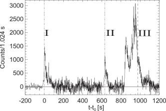
Figure 2: Prompt light curve of GRB 091024 background corrected in energy range 8–1000 keV (Gruber et al., 2011).

There are three emission episodes separated by two periods of quiescence or low activity. Because of the irregularity of the background level, from GBM data it is not possible to understand if there is a continuous activity of the central engine between the episodes or it is completely switched off. Instead, the Konus–Wind data show a low level emission in the period between the pulses (Virgili et al. 2013). The main parameters obtained from the analysis of Gruber et al. (2011) and Virgili et al. (2013) are shown in Tab. 1. These parameters are obtained by fitting the prompt spectrum in each episode with a power–law with a high energy cut–off.

Episode	$t-t_{0}$	$T_{90}$	$E_{p}$	$\alpha$	$\mathcal{F}$	$E_{\rm ISO}$
	[s]	[s]	keV		[$10^{-5}\mbox{ erg}/\mbox{cm}^{2}]$	[$10^{52}$ erg]
I	$-3.8:67.8$	$72.6\pm 1.8$	$412^{+69}_{-53}$	$0.92\pm 0.07$	$1.81\pm 0.07$	$6.3\pm 0.2$
II	$622.7:664.7$	$44.5\pm 5.4$	$371^{+111}_{-71}$	$1.17\pm 0.07$	$0.79\pm 0.04$	$2.8\pm 0.1$
III	$838.8:1070.2$	$150\pm 10$	$278^{+22}_{-18}$	$1.38\pm 0.02$	$6.73\pm 0.09$	$23.6\pm 0.3$

Table 1: Fit parameters of the three episodes of GRB 091024. The model fit is a cut–off power–law. Fluence between 8 keV and 40 MeV (Gruber et al., 2011).

In the following section, we interpret the episodes I and II as emission due to the precursors and episode III as the main event, using the definition of precursor of Burlon et al. (2008).

3.2 Optical Afterglow

We study the optical afterglow in $R^{\prime}$ band (filter peak frequency $\nu=4.84\times 10^{14}$ Hz). The light curve is showed in Fig. 3.

There are two main peaks at $t_{\rm obs}\simeq 500$ s and $t_{\rm obs}\simeq 2,500$ s, and a small rebrightening at $t_{\rm obs}\simeq 5,000$ s.

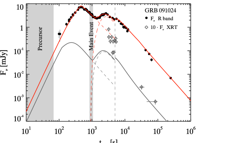
Figure 3: Afterglow light curve of the optical flux in mJy ($R^{\prime}$ band, $\nu=4.84\times 10^{14}$ Hz, black dots) of GRB 091024 compared with the proposed model (red solid line). The afterglow emission of the precursor and the main event are shown by the red dashed lines. The vertical black dashed line represents the time when the two fireballs (of the precursor and of the main event) collide and merge in a new reborn fireball that decelerates in the external CBM. The grey diamonds show the XRT X–ray emission at 1 keV multiplied by 10, compared with the prediction of the model for that frequency. The grey regions show the time of the precursor and the main event prompt emission.

3.3 X–ray Afterglow

The X–ray emission of GRB 091024 has been observed by XRT only since about $3,000$ s after the trigger. The XRT data (flux density at 1 keV) have been retrieved from the Swift Burst Analyzer. X–ray data are shown in Fig. 3 (grey diamonds). It can be seen that the first part of this light curve is rather different from the optical light curve (see also the recent study in D’Avanzo et al. 2012). This indicates that the optical and X–ray fluxes have a different origin (the X–ray flux could be late prompt emission, as suggested by e.g. Ghisellini et al. 2009). However, the last two X–ray points do describe a decay consistent with the optical one, indicating the possibility that these two data points belong to the same mechanism of the optical afterglow (forward external shock).

3.4 Data Interpretation

To interpret the optical afterglow data, we applied this procedure dividing the light curve in three different time bins.

1. $t_{\rm obs}\lesssim 900$ s: Here the afterglow light curve is produced only by the interaction of the fireball of the precursor and the external medium (deceleration of fireball I).

2. $900$ s $\lesssim t_{\rm obs}\lesssim 5,000$ s: The afterglow light curve is given by the superposition of the last part of the afterglow produced by the precursor (fireball I) and the one produced by the main event (fireball II).

3. $t_{\rm obs}\gtrsim 5,000$ s: Here the afterglow light curve is produced by the merger (fireball I+II) of the two fireballs.

We interpret the first peak as produced by the deceleration of fireball I, in the external homogeneous medium. Since this optical emission occurs between the prompt emission of the precursor and the prompt emission of the main event, we can affirm that it cannot be the forward shock afterglow emission of the main event, since its fireball has not been released yet by the central engine.

The second peak is due to the deceleration of fireball II (main event) in the pre–accelerated medium injected by the central engine. The third peak corresponds with the merging of fireballs I and II. After the merging, the merged fireball I+II continues to decelerate in the external circumburst medium (that is not pre–accelerated), so it will produce a more intense and efficient emission. This medium jump causes a discontinuity in the light curve, alias the third peak.

The second precursor, formerly labelled as Episode II, is less energetic than the first one, and, more importantly, its prompt emission is very close in time to the main event. We thus expect that its fireball has not enough time to produce its own afterglow before being reached by the fireball of the main event. We confirm this expectation studying the contribution of the fireball of the second precursor in the Appendix. There we show that the second precursor afterglow emission can be neglected for small values of the initial Lorentz factor of the associated fireball (hereafter labelled as $\Gamma_{0,\rm p,II}$). Therefore, for the sake of simplicity, we will neglect the second precursor in the following, but we add its kinetic energy to the fireball of the main event, i.e.:

$$E_{\rm k,m}=(E_{\rm ISO,II}+E_{\rm ISO,III})/\eta$$ (38)

where $E_{\rm ISO,II}$ and $E_{\rm ISO,III}$ are respectively the isotropic equivalent energy of the Episode II (the second precursor) and the Episode III (the main event) and $\eta$ is the efficiency of conversion of the kinetic energy in radiative energy. The values of $E_{\rm ISO}$ are listed in Tab. 1.

4 Results

4.1 Optical Afterglow results

Fig. 3 shows the optical afterglow light curve compared with the model. There is a very good agreement between the model and the data. The values of the parameters used for the solution of the Fig. 3 are shown in Tab. 2 (fireballs parameters) and in Tab. 3 (medium parameters). A value $n=3\mbox{ cm}^{-3}$ of the circumburst density provides a good agreement between model and data. This value is compatible with the known distribution of the circumburst density (see Panaitescu & Kumar, 2002, Ghisellini et al., 2009 and Cenko et al., 2011).

Portion	$\Gamma_{0}$	$\Gamma_{\rm merg}$	$\epsilon_{e}$	$\epsilon_{B}$	$p$
I	$130$	…	$0.023$	$6.0\times 10^{-4}$	$2.7$
II	$73$	…	$0.028$	$0.017$	$2.5$
III	…	$39.9$	$0.0045$	$0.003$	$2.6$

Table 2: Model parameters for the three portions of the light curve: I) Precursor afterglow emission, II) Main Event afterglow emission, III) Afterglow emission produced after the merger of the precursor and the main event fireball.

$n_{0}$	$7.7\times 10^{7}$	cm-3
$s$	$1$
$\gamma_{0}$	$250$
$g$	$0.25$

Table 3: Parameters of the medium injected by the central engine in the quasi–quiescence phases (for $R_{0}=10^{11}$ cm, see Eqs. 1).

The values of the kinetic energy of the precursor and the main event have been computed from the prompt light curve see Tab. 1), assuming an efficiency $\eta=0.2$, resulting in $E_{\rm k,p}\simeq 3\times 10^{53}$ erg and $E_{\rm k,m}\simeq 1.3\times 10^{54}$ erg (according with the Eq. 38, $E_{\rm k,m}$ includes also the energy of the second precursor, previously called as “Episode II”).

It is not straightforward to explicit analytically the dependence of the predicted flux from the model parameters. However, we have explored numerically the effects of changing the most relevant parameters around the values leading to the curves shown in Fig. 3, listed in Tabs. 2 and 3.

The precursor parameters (especially $\Gamma_{0\rm,p}$) are well constrained by the position of the first optical peak (see also §2.5, where we show the connection between the precursor parameters and the initial bulk Lorentz factor). Instead, it is more challenging to explore the breadth of combinations of the parameters ($\Gamma_{0,\rm m}$, $\gamma_{0}$, $g$, $n_{0}$, $s$) of the main event, since the corresponding afterglow emission is obtained by the interaction with a non–standard medium.

To understand how much these parameters are reliable, we examined a narrow range of the space parameter around them, studying how the second peak of the afterglow changes. Fig. 4 shows the variations of the optical light curve if we vary the Lorentz factor parameters (i.e. $\Gamma_{0,\rm m}$, $\gamma_{0}$ and $g$) by $\sim 4\%$ and the injected medium density parameters (i.e. $n_{0}$ and $s$) by $\sim 2\%$ around the best values. Fig. 4 shows how the light curves are strongly modified even for modest changes of the parameters. Although we made a good exploration of this particular range of the parameter space, we cannot exclude that with a complete study of the parameter space, we could find other combinations of parameters that can reproduce a similar light curve.

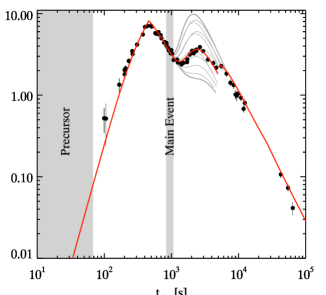
Figure 4: Afterglow light curve of the optical flux of GRB 091024 compared with the proposed model. The best combination of the parameters is represented by the red solid line, the grey lines show how the light curve changes if the parameters are modified in a narrow range (see text in §4.1). The grey regions show the time of the precursor and the main event prompt emission.

4.1.1 Precursor analysis

In this section we will focus on the solution for the optical light curve of the precursor.

At early times, the flux grows with a slope steeper than $t^{2}$, becoming $\propto t^{2}$ before the peak. As described in §2.4, the fast rising argues in favour of a homogeneous circumburst medium. Then there is a very (and unusual) sharp peak followed by a flux decay steeper than $t^{-1}$. In Fig. 5 we show a detail of the optical light curve of the precursor afterglow, the break frequencies $\nu_{\rm i}$ and $\nu_{\rm c}$ and the Lorentz factor of the precursor fireball as a function of the observed time $t_{\rm obs}$.

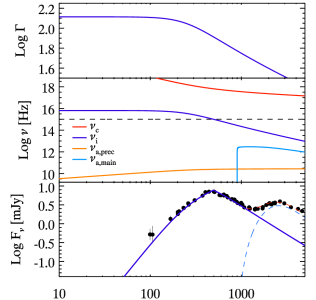
Figure 5: Afterglow emission from the precursor of GRB 091024. Top panel: Lorentz factor $\Gamma$ as a function of the observed time $t_{\rm obs}$. Mid panel: the injection and cooling rest frame frequencies ($\nu_{\rm i}$ and $\nu_{\rm c}$ respectively) and the rest frame self–absorption frequencies for the precursor shock ($\nu_{\rm a,prec}$) and the main event shock ($\nu_{\rm a,main}$) as a function of $t_{\rm obs}$. The dashed line represents the rest frame frequency of observation ($\nu=10^{15}$ Hz). All the frequencies are shown rest frame, i.e. corrected for the cosmological redshift. Bottom panel: optical ($R^{\prime}$ band) light curve of the afterglow emission of the precursor (solid line) and main event light curve (dashed lines). Note that the afterglow peak corresponds at the passage of the injection frequency $\nu_{\rm i}$.

To reproduce the sharpness of the optical peak, we require that it is due not only to the deceleration of the fireball, but also by the transition of the injection frequency $\nu_{\rm i}$. Moreover, we note that $\nu_{\rm i}<\nu_{\rm c}$ always, so the afterglow emission of the precursor is always in the slow cooling regime. We stress that the sharpness of the peak, interpreted as the passage of $\nu_{\rm i}$ simultaneously with the deceleration time, is not a common property of the afterglow onset, but a feature of this specific burst. Therefore, it should not be considered by a weakness of our model.

4.1.2 Self–absorption

In §2.3.1 we claimed that we can neglect the self–absorbed part of the spectrum. This approximation is justified only if the observed frequency $\nu$ is larger than the self–absorption frequency: $\nu>\nu_{\rm a}$. We compute $\nu_{\rm a}$ for the precursor and the main event afterglow emission, using Eq. 21. The result is shown in the middle panel in Fig. 5.

Both self–absorption frequencies are always much smaller than the frequency of observation $\nu$. This justifies our assumed approximation. Moreover, since the self–absorption frequency of the precursor is smaller than the self–absorption frequency of the second (main event) shock, there is no further absorption of main event photons by the precursor shock. In conclusion, self–absorption does not affect the optical emission at all the considered times.

4.2 A consistency check: the X–ray Afterglow

We compare the XRT data sampling at 1 keV (Fig. 3, grey diamonds) and the light curve at 1 keV generated by the same model interpreting the optical light curve.

As mentioned in §3.3, at early times the X–ray emission is very different from the optical counterpart, and is probably due to a different mechanism. Conversely, the last two points show a decay of the X–ray flux compatible with the behaviour of the optical flux and consistent with model predictions. Therefore, the model X–ray flux is required to be below the initial X–ray data points, and be close to the last two X–ray points. This is indeed what we find, shown in Fig. 3.

5 Discussion

Since the general properties of precursors are very similar to the ones of the main events, it is natural to assume that precursors and main events are produced by the same central engine. The energetics of the precursors is less than, but close to, the energetic of the main event, and this implies that the also the precursor generates its own fireball, that produces the first afterglow. As far as we know, this is the first time that the consequences of this scenario are explored. The onset of the first afterglow is linked to the energetics and the bulk Lorentz factor of the precursor, not the ones of the main event, and to the circumburst density. The main event launches a second, more powerful, fireball. It will run into a moving medium, producing afterglow emission not through a standard external forward shock, but with a less efficient kind of internal shock. The onset of this afterglow will then occur at a later time (the fireball takes longer to decelerate). The onset time will still depend on the energetics and the bulk Lorentz factor of the fireball, but in a different way than predicted by the standard theory. In addition, it will depend also on the density and velocity of the surrounding medium, ejected during the quiescent phase (i.e. the time interval between the precursor and the main event). Finally, when the second fireball reaches the first, we will have a third peak of the afterglow light curve. This can be considered as a refreshed shock. After the third peak, we have the standard behaviour.

We believe that this three-peak light curve is a distinguishing feature of the afterglow of the bursts with precursors in this idealized and simple case. There could be in fact a variety of cases: for instance, the burst could have more than one precursor (and this would increase the number of peaks in the light curve). Consider also that the second peak could not emerge, being hidden by the light curve produced by the first fireball (especially when the quiescent phase is short), or else the second fireball might not decelerate before catching the second fireball.

The proposed model well explain the optical afterglow of GRB 091024, which is otherwise difficult to understand (see the discussion in Virgili et al. 2013). Even if admittedly simplified (we have neglected the reverse shock and treated only the case of an homogeneous CBM), the model accounts for the observed optical light curve in a quite logical and simple way.

Appendix: second precursor of GRB 091024

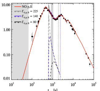
Figure 6: How the afterglow light curve of GRB 091024 changes if we consider also the second precursor. Red solid line: the afterglow without the second precursor; grey dashed line: the afterglow of the second precursor with $\Gamma_{0,\rm p,II}=225$, grey solid line: the resulting total afterglow light curve; blue dashed line: the afterglow of the second precursor with $\Gamma_{0,\rm p,II}=140$, blue solid line: the resulting total afterglow light curve; black dashed line: the afterglow of the second precursor with $\Gamma_{0,\rm p,II}=80$, black solid line: the resulting total afterglow light curve (it is almost coincident with the red solid line). The vertical dotted lines show when the second precursor fireball is reached by the main event fireball, stopping the second precursor afterglow emission. They differ according to the $\Gamma_{0,\rm p,II}$ used.

In this section we analyse how the optical light curve of GRB 091024 changes if we consider also the afterglow produced by the second precursor, formerly labeled as “Episode II”.

We will show that the contribution of this precursor is negligible as long as its initial bulk Lorentz factor ($\Gamma_{0,\rm p,II}$) is smaller than a limit value $\Gamma_{\rm lim}$ that is determined numerically.

If we consider also the second precursor in the calculation, the number of parameters increases (we must add the initial Lorentz factor of the second precursor fireball $\Gamma_{0,\rm p,II}$ and the shock parameters $\epsilon_{\rm e}$, $\epsilon_{\rm B}$ and $p$), but the number of observable quantities does not change. Therefore, the parameters of this second precursor are much less constrained than the other.

We are then forced to use a fixed value for the shock parameters (the same used for the main event afterglow emission) and vary the initial Lorentz factor. Fig. 6 shows how the light curve varies if we consider also the emission of the second precursor, for different initial Lorentz factors. We can see that if $\Gamma_{0,\rm p,II}\lower 3.22916pt\hbox{$\sim$}\hbox to0.0pt{\hss\raise 1.1625pt\hbox{$<$}}140$, the second precursor afterglow is negligible. In any case, since the fireball of the second precursor is released very close to the fireball of the main event, the afterglow of this precursor can not last longer than $\sim 2,300$ s after the trigger, and it cannot influence significantly the parameters concerning the injected medium and the bulk Lorentz factor of the fireball associated to the main event.

References

- [] Ackermann M., Asano K., Atwood W.B., et al., 2010, ApJ, 716, 1178
- [] Bernardini M.G., Campana S., Ghisellini G. et al., 2014, MNRAS, 439, L80
- [] Bernardini M.G., Campana S., Ghisellini G. et al., 2013, ApJ, 775, 67
- [] Bissaldi E. & Connaughton V., 2009, GCN circular N. 10070
- [] Bouvier A., McEnery J., Chiang J., Kocevski D., Moretti E., Vasileiou V. & Piron F., 2009, GCN circular N. 10114
- [] Burlon D., Ghirlanda G., Ghisellini G., Lazzati D., Nava L., Nardini M. & Celotti A. 2008, ApJ, 685, L19
- [] Burlon D., Ghirlanda G., Ghisellini G., Greiner J. & Celotti A. 2009, A&A, 505, 569
- [] Cenko S.B., Kasliwal M., Harrison F.A., et al., 2006, ApJ, 652, 490
- [] Cenko S.B., Kasliwal M.M. & Kulkarni S.R., 2009, GCN circular N. 10093
- [] Cenko S.B., Frail D.A., Harrison F.A., et al., 2011, ApJ, 732, 29
- [] Cucchiara A., Fox D. & Tanvir N., 2009, GCN circular N. 10065
- [] D’Avanzo P., Salvaterra R., Sbaruffatti B., et al., 2012, MNRAS, 425, 506
- [] Daigne F. & Mochkovitch R., 2002, MNRAS, 336, 1271
- [] Frail D.A., Kulkarni S.R., Sari R., et al., 2001, ApJ, 562, L55
- [] Ghirlanda G., Ghisellini G., & Lazzati D., 2004, ApJ, 616, 331
- [] Ghirlanda G., Nava L., Ghisellini G., Celotti A., Burlon D., Covino S., Melandri A., 2012, MNRAS, 420, 483
- [] Ghisellini G., Ghirlanda G., Nava L. & Celotti A., 2010, MNRAS, 403, 926
- [] Ghisellini G., Nardini M., Ghirlanda G. & Celotti A., 2009, MNRAS, 393, 253
- [] Golenetskii R., Aptekar R., Mazets E., Pal’shin V., Frederiks D., Oleynik P., Ulanov M. & Svinkin D., 2009, GCN Circular N. 10083
- [] Gruber D., Krühler T., Foley S., et al., 2011, A&A, 528, A15
- [] Koshut T.M., Kouveliotou C., Paciesas W.S., et al., 1995, ApJ, 452, 145
- [] Lazzati D., 2005, MNRAS, 357, 722
- [] Lazzati D., & Begelman M.C., 2005, ApJ, 629, 903
- [] Lipunova G.V., Gorbovskoy E. S., Bogomazov A.I., & Lipunov V.M., 2009, MNRAS, 397, 1695
- [] Lyutikov M., & Blandford R., 2003 [arXiv:astro-ph/0312347]
- [] Marshall F.E., Baumgartner W.H., Beardmore A.P. et al. 2009, GCN Circular N. 10062
- [] Meszaros P., & Rees M. J., 2000, ApJ, 530, 292
- [] Nava L., Sironi L., Ghisellini G., Celotti A., & Ghirlanda G., 2013, MNRAS, 433, 2107
- [] Page K.L. & Marshall F.E., 2009, GCN circular N. 10069
- [] Panaitescu A. & Kumar P., 2000, ApJ, 543, 66
- [] Panaitescu A. & Kumar P., 2002, ApJ, 571, 779
- [] Ramirez–Ruiz E., MacFadyen A.I., & Lazzati D. 2002, MNRAS, 331, 197
- [] Rees M.J. & Mészáros P., 1998, ApJ, 496, L1
- [] Ruffini R., Bianco C.L., Fraschetti F., Xue S.–S., & Chardonnet P.. 2001, ApJ, 555, L113
- [] Sari R., 1997, ApJ, 489, L37
- [] Sari R. & Esin A.A., 2001, ApJ, 548, 787
- [] Sari R., Piran T. & Narayan R., 1998, ApJ, 497, L17
- [] Troja E., Rosswog S. & Gehrels, N., 2010, ApJ, 723, 1711
- [] Updike A.C., Hartmann D.H., Milne P.A. & Williams G.G., 2009, GCN circular N. 10074
- [] Virgili F.J., Mundell C.G., Pal’shin V. et al., 2013, ApJ, 778, 54
- [] Wang, X.-Y., & Mészáros, P. 2007, ApJ, 670, 1247