Next-to-leading order QCD corrections to $ZZ$ production in association with two jets

Abstract

We present the first calculation of next-to-leading order QCD corrections to QCD-induced $ZZ$ production in association with two jets at hadron colliders. Both $Z$ bosons decay leptonically with all off-shell effects, virtual photon contributions and spin-correlation effects fully taken into account. This process is an important background to weak boson scattering, to the measurement of quartic gauge couplings and to searches for signals of new physics beyond the Standard Model. As expected, the next-to-leading order corrections reduce significantly the scale uncertainty and show a non-trivial phase space dependence in kinematic distributions. Our code will be publicly available as part of the parton level Monte Carlo program VBFNLO.

1 Introduction

With the first measurement ATLAS001 of same-sign $W^{\pm}W^{\pm}jj$ vector boson production at the LHC ATLAS experiment at $\sqrt{s}=8\,\mathrm{TeV}$, the program to test $VV\to VV$ scattering and the EW quartic gauge couplings has been started. The data are in agreement with the Standard Model (SM) prediction Jager:2009xx ; Denner:2012dz ; Melia:2010bm ; Campanario:2013gea and provide the first evidence for electroweak (EW) gauge boson scattering, namely $W^{\pm}W^{\pm}\to W^{\pm}W^{\pm}$. In this context, the class of processes with two EW gauge bosons and two jets in the final state plays a very important role. Furthermore, these processes are important backgrounds for searching signals of new physics beyond the SM.

From the theoretical side, progress has been made to provide predictions at next-to-leading order (NLO) QCD accuracy. The strategy used so far is first to implement the calculation of the hard processes

$$pp\to VVjj+X,$$ (1)

where both gauge bosons decay leptonically, in a parton level Monte Carlo program, where parton distribution functions and a jet algorithm to cluster final state partons into jets are applied, and then interface it to other programs which can do parton shower and hadronization. From a physical point of view and also due to the complexity of the calculation, it has been traditional to classify the process, Eq. (1), into EW and QCD induced contributions based on the difference in the overall coupling constant at leading order (LO) and calculate them separately. The interference effects between these two contributions are expected to be negligible for most measurements at the LHC. However, if needed, one can calculate these effects at LO using an automated program e.g. Sherpa Gleisberg:2008ta . For a recent discussion on this issue, we refer to Ref. Campanario:2013gea , where the interferences of the same-sign $W^{\pm}W^{\pm}jj$ vector boson production process were studied, which are expected to be maximal because the gluon-initiated subprocesses are absent at LO and both the EW and QCD amplitudes involve only left-chiral quarks and leptons.

The EW-induced channels of order $\mathcal{O}\!\left(\alpha^{4}\right)$ for on-shell production at LO are further classified into “vector boson fusion” (VBF) mechanisms, which are sensitive to the EW quartic gauge couplings and the dynamics of $VV\to VV$ scattering and other contributions including $VVV$ production with one $V$ decaying into two jets. The important message is that the VBF mechanisms can be strongly enhanced if VBF cuts are applied. References for the NLO QCD calculations of the EW-induced channels and the definition of the VBF cuts can be found in Ref. Campanario:2013gea .

In this paper, we consider the $\mathcal{O}\!\left(\alpha^{2}\alpha_{s}^{2}\right)$ QCD-induced mechanism for the process with $ZZjj$ in the final state and will present the first theoretical prediction at NLO QCD accuracy. The NLO QCD computation of the corresponding EW-induced VBF mechanism has been done in Ref. Jager:2006cp . The NLO QCD corrections to the QCD-induced channels are much more difficult because QCD radiation occurs already at LO, leading to complicated topologies (up to hexagons with rank-5 tensor integrals) with non-trivial color structures at NLO. The calculations for $W^{+}W^{-}jj$ production have been presented in Refs. Melia:2011dw ; Greiner:2012im , for the same-sign $W^{+}W^{+}jj$ in Refs. Melia:2010bm ; Campanario:2013gea and for $W^{\pm}Zjj$ in Ref. Campanario:2013qba . Similar calculations with the massless photon in the final state have also been calculated for $\gamma\gamma jj$ Gehrmann:2013bga ; Badger:2013ava ; Bern:2014vza and $W\gamma jj$ Campanario:2014dpa production. Results for $\gamma\gamma jjj$ production at NLO QCD have been very recently presented also in Ref. Badger:2013ava . Results at the total cross section level for on-shell $VVjj$ production have been very briefly reported recently in Ref. Alwall:2014hca .

Our $ZZjj$ calculation with leptonic decays has been implemented within the VBFNLO framework Arnold:2008rz ; Baglio:2014uba , a parton level Monte Carlo program which allows the definition of general acceptance cuts and distributions. As customary in VBFNLO, all off-shell effects, virtual photon contributions and spin-correlation effects are fully taken into account. In this paper, we focus on the four charged-lepton final states. The $l^{+}l^{-}\bar{\nu}\nu$ channels are simpler and can be easily adapted from the four charged-lepton code (e.g. switching off a virtual photon contribution, changing the lepton-Z couplings). This possibility will be available in the next release of VBFNLO.

The outline of this paper is the following. Details of our calculation are provided in Section 2. In Section 3 numerical results for inclusive cross sections and various distributions are given. Conclusions are presented in Section 4 and in Appendix A results at the amplitude squared level for a random phase-space point are provided in order to facilitate comparison with independent calculations.

2 Calculational details

In this paper, we calculate the QCD-induced processes at NLO QCD for the process

$$pp\to l_{1}^{+}l_{1}^{-}l_{2}^{+}l_{2}^{-}jj+X,$$ (2)

at order ${\cal O}(\alpha_{s}^{3}\alpha^{4})$. We assume that all the leptons are massless and $l_{1}\neq l_{2}$.

Figure 1: Representative tree-level Feynman diagrams.

This process is then divided into the contributions

$$pp \to\hat{V}jj+X,$$ (3)

$$pp \to V_{1}V_{2}jj+X,$$ (4)

where $\hat{V}=Z,\gamma^{*}$ with subsequent decay $\hat{V}\to l_{1}^{+}l_{1}^{-}l_{2}^{+}l_{2}^{-}$ and $V_{i}=Z,\gamma^{*}$ with $V_{i}\to l_{i}^{+}l_{i}^{-}$ ($i=1,2$). Some representative Feynman diagrams are shown in Fig. 1. At the LHC, the dominant contribution comes from the process in Eq. (4) with $V_{1}=V_{2}=Z$ because the gauge bosons can be both simultaneously on-shell. For simplicity, we describe the resonating $Z$ propagators with a fixed width and keep the weak-mixing angle real. Moreover, since those leptonic decays of the neutral gauge bosons are consistently included in our calculation by the replacement of the polarization vectors with the corresponding effective currents, we will sometimes refer to the process in Eq. (2) as $ZZjj$ production.

We use the Feynman diagrammatic approach and classify at LO the above contributions into $4$-quark and $2$-quark-$2$-gluon amplitudes

$$uu \to uu\;V_{1}V_{2},$$

$$uc \to uc\;V_{1}V_{2},$$

$$ud \to ud\;V_{1}V_{2},$$

$$dd \to dd\;V_{1}V_{2},$$

$$ds \to ds\;V_{1}V_{2},$$

$$gg \to\bar{u}u\;V_{1}V_{2},$$

$$gg \to\bar{d}d\;V_{1}V_{2},$$ (5)

where the sub-dominant processes in Eq. (3) and the leptonic decays are implicitly included.

From these seven generic subprocesses we can obtain all the amplitudes of other subprocesses via crossing or/and exchanging the partons. We work in the 5-flavor scheme, i.e. external bottom-quark contributions with $m_{b}=0$ are included. Subprocesses with external top quarks are excluded, but virtual top-loop contributions are included in our calculation as specified below.

At NLO QCD, there are the virtual and the real-emission corrections. We use dimensional regularization 'tHooft:1972fi to regularize the ultraviolet (UV) and infrared (IR) divergences and use an anticommuting prescription of $\gamma_{5}$ Chanowitz:1979zu . The UV divergences of the virtual amplitude are removed by the renormalization of $\alpha_{s}$. Both the virtual and the real corrections are infrared divergent. These divergences are canceled using the Catani-Seymour prescription Catani:1996vz such that the virtual and real corrections become separately numerically integrable. The real emission contribution includes, allowing for external bottom quarks, $275$ subprocesses with seven particles in the final state.

Figure 2: Selected Feynman diagrams contributing to the virtual amplitudes.

The virtual amplitudes are more challenging involving up to six-point rank-five one-loop tensor integrals appearing in the $2$-quark-$2$-gluon virtual amplitudes. There are $42$ six-point diagrams for the last subprocess in Eq. (5). Since the kinematics does not change if a $Z$ boson is replaced by a virtual photon, the same hexagon integrals occur in the $ZZ$, $Z\gamma^{*}$, $\gamma^{*}Z$ and $\gamma^{*}\gamma^{*}$ contributions and hence are reused for optimization. The $4$-quark group is simpler with $24$ generic hexagons for the first subprocess in Eq. (5). For the other $4$-quark subprocesses with different flavors there are $12$ hexagons.

In Fig. 2, we highlight some contributions to the virtual amplitude. Diagrams including a closed-quark loop with gluons attached to it, e.g. the last diagram of Fig. 2, are taken into account. However, we do not include closed-quark loops where the $Z/\gamma^{*}$ vector bosons or/and the Higgs boson are directly attached to them. This set of diagrams forms a gauge invariant subset and contributes at the few per mille level to the NLO results Greiner:2012im , and hence are negligible for all phenomenological purposes. On the other hand, the discarded diagrams, which include the loop-induced $gg\to H(\to ZZ)jj$ channels, can be regarded as a new mechanism, which also receives contributions from $gg\to ZZgg$. To properly take into account these loop-induced channels one has to calculate the square of those amplitudes, which formally are of higher-order but can be somewhat enhanced by the Higgs resonance and the large gluon luminosity at the LHC. Part of those amplitudes can be obtained from the $gg\to ZZg$ calculation presented in Ref. Campanario:2012bh . This effect is expected to be at the few percent level, which is of similar size as the interferences between the EW and QCD induced mechanisms discussed in the introduction. We note that NLO EW corrections are also at the same level.

The evaluation of scalar integrals is done following Refs. 'tHooft:1978xw ; Bern:1993kr ; Dittmaier:2003bc ; Nhung:2009pm ; Denner:2010tr . The tensor coefficients of the loop integrals are computed using the Passarino-Veltman reduction formalism Passarino:1978jh up to the box level. For pentagons and hexagons, we use the reduction formalism of Ref. Denner:2005nn (see also Refs. Campanario:2011cs ; Binoth:2005ff ).

Our calculation has been carefully checked as follows. The present calculation shares a large common part with our previous $W^{\pm}Zjj$ calculation Campanario:2013gea , which has been validated at the amplitude level performing two independent calculations. For the real-emission part, the structure of QCD radiation and therefore the implementation of the Catani-Seymour dipole subtraction method is the same. The only difference is the computation of the tree-level amplitudes. Using two independent codes, we have crosschecked the real-emission amplitudes and the corresponding subtraction terms at a random phase-space point and obtained 10 digit agreement with double precision. Similarly, the integrated part of the dipole subtraction term defined in Ref. Catani:1996vz has been validated at the integration level. Moreover, the real-emission contribution including the subtraction terms has been crosschecked against Sherpa Gleisberg:2008ta ; Gleisberg:2008fv and agreement at the per mill level was found. For the virtual part, we have again checked the whole virtual amplitudes with two independent calculations and obtained full agreement, typically $6$ to $12$ digits with double precision, at the amplitude level. The first implementation uses FeynArts-3.4 Hahn:2000kx and FormCalc-6.2 Hahn:1998yk to obtain the virtual amplitudes. The in-house library LoopInts is used to evaluate the scalar and tensor one-loop integrals.

For the second implementation, which will be publicly available via the VBFNLO program and is the one used to obtain the numerical results presented in the next section, we use the in-house library presented in Ref. Campanario:2011cs to compute the amplitudes and evaluate the tensor integrals.

Furthermore, we closely follow the strategy described in Refs Campanario:2011cs ; Campanario:2012bh ; Campanario:2013gea ; Campanario:2014dpa to optimize the code and to deal with numerical instabilities occurring in the numerical evaluation of the virtual part. With this method, we obtain the NLO inclusive cross section with statistical error of $1\%$ in 3.5 hours on an Intel $i5$-$3470$ computer with one core and using the compiler Intel-ifort version $12.1.0$. The distributions shown below are based on multiprocessor runs with a total statistical error of 0.03%.

3 Numerical results

As input parameters, we use $M_{W}=80.385{\,\mathrm{GeV}}$, $M_{Z}=91.1876{\,\mathrm{GeV}}$, $m_{t}=173.1{\,\mathrm{GeV}}$ and $G_{F}=1.16637\times 10^{-5}{\,\mathrm{GeV}}^{-2}$. The tree-level relations are then used to calculate the weak mixing angle and the electromagnetic coupling constant. We use the MSTW2008 parton distribution functions Martin:2009iq with $\alpha_{s}^{\text{LO}}(M_{Z})=0.13939$ and $\alpha_{s}^{\text{NLO}}(M_{Z})=0.12018$. The $Z$ total width is calculated as $\Gamma_{Z}=2.508905{\,\mathrm{GeV}}$. All fermions but the top quark are approximated as massless. We work in the five-flavor scheme and use the $\overline{MS}$ renormalization of the strong coupling constant with the top quark decoupled from the running of $\alpha_{s}$. However, the top-loop contribution is explicitly included in the virtual amplitudes. We choose inclusive cuts defined as

$$p_{T(j,l)} >20{\,\mathrm{GeV}} |y_{j}| <4.5$$

$$|y_{l}| <2.5 R_{l(l,j)} >0.4,$$ (6)

where the anti-$k_{t}$ algorithm Cacciari:2008gp with a cone radius of $R=0.4$ is used to cluster partons into jets. For the cut on $R_{lj}$, all reconstructed jets are taken into account. We use a dynamical factorization and renormalization scale with the central value

$$\mu_{F}=\mu_{R}=\mu_{0}=\frac{1}{2}\left[E_{T}(jj)+E_{T}(4l)\right],$$ (7)

where $E_{T}=(p_{T}^{2}+p^{2})^{1/2}$ is calculated for the systems of the two tagging jets and of the four leptons. The two tagging jets are defined as the highest transverse-momentum jets. This scale choice is well motivated because the $E_{T}(jj)$ term interpolates between the transverse momenta and the invariant mass of the tagging-jet system. It is therefore similar to the default scale defined in Ref. Campanario:2014dpa . We have checked that the two scale choices indeed produce nearly identical results for various kinematic distributions at both LO and NLO levels. In the following, results for the integrated cross section and for various differential distributions with the above setting will be presented. We sum over all possible combinations of charged leptons of the first two generations, i.e. final states $e^{+}e^{-}\mu^{+}\mu^{-}$, $e^{+}e^{-}e^{+}e^{-}$ and $\mu^{+}\mu^{-}\mu^{+}\mu^{-}$ are all included. Since Pauli-interference effects for the identical lepton channels are neglected, this sum amounts to a factor of two compared to the single $e^{+}e^{-}\mu^{+}\mu^{-}$ result.

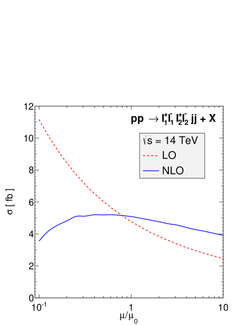
Figure 3: Scale dependence of the LO and NLO cross sections at the LHC. The reference scale $\mu_{0}$ is defined in Eq. (7). All possible combinations of charged leptons of the first two generations are included.

As customary in the framework of perturbative QCD, our NLO results depend on the scales $\mu_{F}$ and $\mu_{R}$. We set them equal for simplicity. The scale dependence of the total cross section at LO and NLO is shown in Fig. 3. At the default scale $\mu_{0}$, we obtain $\sigma_{\text{LO}}=4.7783(3)^{+1.25}_{-0.93}{\,\mathrm{fb}}$ and $\sigma_{\text{NLO}}=5.075(2)^{+0.13}_{-0.30}{\,\mathrm{fb}}$ where the numbers in the parentheses are the statistical errors of the numerical integrations and the other uncertainties are due to $\mu_{0}/2\leq\mu_{F}=\mu_{R}\leq 2\mu_{0}$ variations. As expected, the scale dependence around the central value $\mu_{0}$ is significantly reduced when the NLO contribution is included.

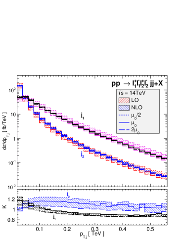
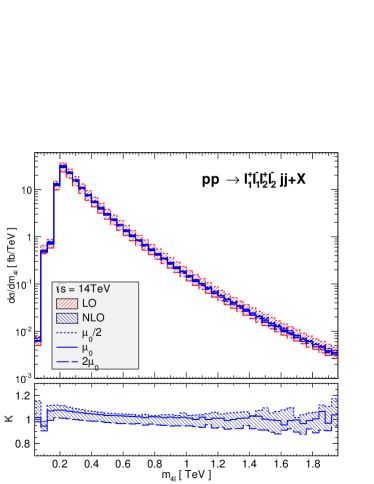
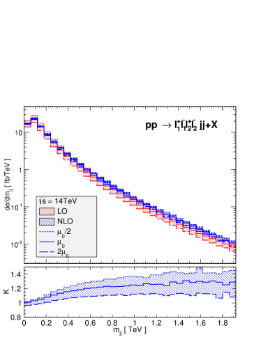
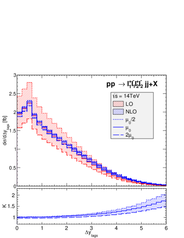
Figure 4: Differential cross sections with inclusive cuts for the transverse momenta (top left), the invariant mass of the four-lepton system (top right) and of the two tagging jets (bottom left). The distributions of the rapidity separation between the two jets are in the bottom right panel. The bands describe $\mu_{0}/2\leq\mu_{F}=\mu_{R}\leq 2\mu_{0}$ variations. The $K$-factor bands are due to the scale variations of the NLO results, with respect to $\sigma_{\text{LO}}(\mu_{0})$. The solid lines are for the central scale while the dotted and dashed lines correspond to $\mu_{0}/2$ and $2\mu_{0}$, respectively. All possible combinations of charged leptons of the first two generations are included.

We now study the phase space dependence of the NLO QCD corrections. In Fig. 4, we display the distributions of the transverse momenta (top left) and the invariant mass (bottom left) of the two hardest jets and the invariant mass of the four-lepton system (top right). The distributions of the rapidity separation between the two jets are in the bottom right panel. The $K$ factors, defined as the ratio of the NLO to the LO results, are shown in the small panels. To give a measure of scale uncertainty, we vary the scales in the range $\mu_{0}/2\leq\mu_{F}=\mu_{R}\leq 2\mu_{0}$ and plot the LO and NLO bands in the large panels. The $K$-factor bands are due to the scale variations of the NLO results, with respect to $\sigma_{\text{LO}}(\mu_{0})$. As expected, the scale uncertainties for all the distributions are significantly reduced at NLO. We observe non-trivial behaviors of the $K$ factors, varying from $0.8$ to $1.7$ for the default scale. The rapidity-separation distribution shows that NLO QCD corrections are important at large separation ($\Delta y_{\text{tags}}>4$), which is the phase space region selected by VBF cuts Jager:2006cp to enhance $VV\to VV$ scatterings.

4 Conclusions

In this paper, we have presented first results at NLO QCD for the four charged-lepton $l_{1}^{+}l_{1}^{-}l_{2}^{+}l_{2}^{-}$ production in association with two jets at the LHC via QCD-induced mechanisms at order ${\cal O}(\alpha_{s}^{3}\alpha^{4})$. The final-state leptons are created via a virtual photon or a $Z$ boson. The dominant contribution comes from the phase space regions where two intermediate $Z$ bosons are simultaneously resonant, therefore this process is usually referred to as $ZZjj$ production. All off-shell effects, virtual photon contributions and spin-correlation effects are fully taken into account. We have shown that the NLO QCD corrections are important and hence should be taken into account for precise measurements at the LHC. With this result the calculation of NLO QCD corrections to the production of two massive gauge bosons together with two jets is now practically complete.

Our code will be publicly available as part of the VBFNLO program Arnold:2008rz ; Baglio:2014uba , thereby further studies of the QCD corrections with different kinematic cuts can be easily done.

Appendix A Results at one phase-space point

In this appendix, results at a random phase-space point are provided for comparison with future independent calculations. We focus on the virtual amplitudes, which are most complicated, of the seven benchmark subprocesses in Eq. (5). The amplitudes of all other subprocesses can be obtained via crossing or/and exchanging the partons. The phase-space point for the process $j_{1}j_{2}\to j_{3}j_{4}e^{+}e^{-}\mu^{+}\mu^{-}$ is given in Table 1, which is the same as the one in Ref. Campanario:2013gea .

Table 1: Momenta (in GeV) at a random phase-space point for $j_{1}j_{2}\to j_{3}j_{4}e^{+}e^{-}\mu^{+}\mu^{-}$ subprocesses.

	$E$		$p_{x}$		$p_{y}$		$p_{z}$
$j_{1}$	18.	3459102072588	0.	0	0.	0	18.	3459102072588
$j_{2}$	4853.	43796816526	0.	0	0.	0	-4853.	43796816526
$j_{3}$	235.	795970274883	-57.	9468743482139	-7.	096445419113396$\times 10^{-15}$	-228.	564869022223
$j_{4}$	141.	477229270568	-45.	5048903376581	-65.	9221967646567	-116.	616359620580
$e^{+}$	276.	004829895761	31.	4878768361538	-8.	65306166938040	-274.	066240646098
$e^{-}$	1909.	28515244344	29.	6334571080402	40.	1409467910328	-1908.	63311192893
$\mu^{+}$	2241.	46026948104	28.	1723094714198	30.	2470561132914	-2241.	07910976778
$\mu^{-}$	67.	7604270068059	14.	1581212702582	4.	18725552971283	-66.	1323669723852

Table 2: QCD interference amplitudes $2\text{Re}(\mathcal{A}_{\text{NLO}}\mathcal{A}^{*}_{\text{LO}})$ for $j_{1}j_{2}\to j_{3}j_{4}e^{+}e^{-}\mu^{+}\mu^{-}$ subprocess.

	$1/\epsilon^{2}$		$1/\epsilon$		finite
			$uu\to uu$
I operator	2.	8915745669$\times 10^{-6}$	-1.	4951973738$\times 10^{-6}$	6.	947191076$\times 10^{-7}$
loop	-2.	8915745669$\times 10^{-6}$	1.	4951973738$\times 10^{-6}$	1.	215325266$\times 10^{-5}$
I+loop	-3.	7$\times 10^{-17}$	3.	2$\times 10^{-18}$	1.	284797177$\times 10^{-5}$
			$uc\to uc$
I operator	5.	3681641565$\times 10^{-7}$	1.	6010109373$\times 10^{-7}$	-1.	216280481$\times 10^{-7}$
loop	-5.	3681641568$\times 10^{-7}$	-1.	6010109374$\times 10^{-7}$	3.	231794702$\times 10^{-6}$
I+loop	-3.	2$\times 10^{-17}$	-1.	7$\times 10^{-17}$	3.	110166654$\times 10^{-6}$
			$ud\to ud$
I operator	1.	4782975725$\times 10^{-6}$	4.	4089012802$\times 10^{-7}$	-3.	349421572$\times 10^{-7}$
loop	-1.	4782975726$\times 10^{-6}$	-4.	4089012788$\times 10^{-7}$	6.	305527891$\times 10^{-6}$
I+loop	-3.	7$\times 10^{-17}$	1.	4$\times 10^{-16}$	5.	970585734$\times 10^{-6}$
			$dd\to dd$
I operator	4.	4102124035$\times 10^{-6}$	-2.	278825350$\times 10^{-6}$	1.	0675989830$\times 10^{-6}$
loop	-4.	4102124036$\times 10^{-6}$	2.	278825350$\times 10^{-6}$	1.	8933497562$\times 10^{-5}$
I+loop	-8.	2$\times 10^{-17}$	-1.	1$\times 10^{-16}$	2.	0001096545$\times 10^{-5}$
			$ds\to ds$
I operator	8.	186414665$\times 10^{-7}$	2.	4415310398$\times 10^{-7}$	-1.	854819651$\times 10^{-7}$
loop	-8.	186414665$\times 10^{-7}$	-2.	4415310395$\times 10^{-7}$	5.	284395333$\times 10^{-6}$
I+loop	-7.	3$\times 10^{-17}$	2.	7$\times 10^{-17}$	5.	098913368$\times 10^{-6}$
			$gg\to\bar{u}u$
I operator	1.	3039060448$\times 10^{-8}$	-9.	9737377238$\times 10^{-9}$	8.	78497860$\times 10^{-11}$
loop	-1.	3039060448$\times 10^{-8}$	9.	9737377219$\times 10^{-9}$	3.	21106128$\times 10^{-9}$
I+loop	-3.	0$\times 10^{-20}$	-2.	0$\times 10^{-18}$	3.	29891107$\times 10^{-9}$
			$gg\to\bar{d}d$
I operator	1.	53496729122$\times 10^{-8}$	-1.	22781617391$\times 10^{-8}$	1.	05371064$\times 10^{-9}$
loop	-1.	53496729122$\times 10^{-8}$	1.	22781617377$\times 10^{-8}$	2.	17252400$\times 10^{-9}$
I+loop	-3.	4$\times 10^{-20}$	-1.	4$\times 10^{-18}$	3.	22623464$\times 10^{-9}$

In the following, we provide the squared amplitude averaged over the initial-state helicities and colors. We also set $\alpha=\alpha_{s}=1$ for simplicity. The top quark is decoupled from the running of $\alpha_{s}$, but its contribution is explicitly included in the one-loop amplitudes. All contributions including UV counterterms or a closed-quark loop with gluons attached to it are taken into account. As specified in Section 2, diagrams including a closed-quark loop with the $Z/\gamma^{*}$ or/and the Higgs boson directly attached to it are excluded . At tree level, we get

$$\overline{|\mathcal{A}_{\text{LO}}^{uu\rightarrow uu}|}^{2} =3.40655603126\times 10^{-6},$$

$$\overline{|\mathcal{A}_{\text{LO}}^{uc\rightarrow uc}|}^{2} =6.3242194040\times 10^{-7},$$

$$\overline{|\mathcal{A}_{\text{LO}}^{ud\rightarrow ud}|}^{2} =1.741578298\times 10^{-6},$$

$$\overline{|\mathcal{A}_{\text{LO}}^{dd\rightarrow dd}|}^{2} =5.195659083\times 10^{-6},$$

$$\overline{|\mathcal{A}_{\text{LO}}^{ds\rightarrow ds}|}^{2} =9.644392564\times 10^{-7},$$

$$\overline{|\mathcal{A}_{\text{LO}}^{gg\rightarrow\bar{u}u}|}^{2} =9.4530961185\times 10^{-9},$$

$$\overline{|\mathcal{A}_{\text{LO}}^{gg\rightarrow\bar{d}d}|}^{2} =1.11282506898\times 10^{-8}.$$ (8)

The interference amplitudes $2\text{Re}(\mathcal{A}_{\text{NLO}}\mathcal{A}^{*}_{\text{LO}})$, for the one-loop corrections and the I-operator contribution as defined in Ref. Catani:1996vz , are given in Table 2. For the one-loop integrals, we use the convention

$$T_{0}=\frac{\mu_{R}^{2\epsilon}\Gamma(1-\epsilon)}{i\pi^{2-\epsilon}}\int d^{D}q\frac{1}{(q^{2}-m_{1}^{2}+i0)\cdots},$$ (9)

with $D=4-2\epsilon$. This amounts to dropping a factor ${(4\pi)^{\epsilon}}/{\Gamma(1-\epsilon)}$ both in the virtual corrections and the I-operator. In addition, the conventional dimensional regularization method 'tHooft:1972fi with $\mu_{R}=M_{Z}$ is used. Switching from the conventional dimensional regularization to dimensional reduction method induces a finite shift. This shift can be calculated observing that the sum $|\mathcal{A}_{\text{LO}}|^{2}+2\text{Re}(\mathcal{A}_{\text{NLO}}\mathcal{A}^{*}_{\text{LO}})$ must remain unchanged Catani:1996pk . The shift on the Born amplitude squared is given by the following change in the strong coupling constant, see e.g. Ref. Kunszt:1993sd ,

$$\alpha_{s}^{\overline{DR}}=\alpha_{s}^{\overline{MS}}\left(1+\frac{\alpha_{s}}{4\pi}\right).$$ (10)

The shift on the I-operator contribution can easily be obtained using the rule given in Ref. Catani:1996vz .

- (1) T. A. collaboration, Evidence for electroweak production of in collisions at TeV with the ATLAS detector, .
- (2) B. Jager, C. Oleari, and D. Zeppenfeld, Next-to-leading order QCD corrections to and production via weak-boson fusion, Phys.Rev. D80 (2009) 034022, [0907.0580].
- (3) A. Denner, L. Hosekova, and S. Kallweit, NLO QCD corrections to production in vector-boson fusion at the LHC, Phys.Rev. D86 (2012) 114014, [1209.2389].
- (4) T. Melia, K. Melnikov, R. Rontsch, and G. Zanderighi, Next-to-leading order QCD predictions for production at the LHC, JHEP 1012 (2010) 053, [1007.5313].
- (5) F. Campanario, M. Kerner, L. D. Ninh, and D. Zeppenfeld, Next-to-leading order QCD corrections to and production in association with two jets, Phys.Rev. D89 (2014) 054009, [arXiv:1311.6738].
- (6) T. Gleisberg, S. Hoeche, F. Krauss, M. Schonherr, S. Schumann, et al., Event generation with SHERPA 1.1, JHEP 0902 (2009) 007, [0811.4622].
- (7) B. Jager, C. Oleari, and D. Zeppenfeld, Next-to-leading order QCD corrections to Z boson pair production via vector-boson fusion, Phys.Rev. D73 (2006) 113006, [hep-ph/0604200].
- (8) T. Melia, K. Melnikov, R. Rontsch, and G. Zanderighi, NLO QCD corrections for pair production in association with two jets at hadron colliders, Phys.Rev. D83 (2011) 114043, [1104.2327].
- (9) N. Greiner, G. Heinrich, P. Mastrolia, G. Ossola, T. Reiter, et al., NLO QCD corrections to the production of plus two jets at the LHC, Phys.Lett. B713 (2012) 277–283, [1202.6004].
- (10) F. Campanario, M. Kerner, L. D. Ninh, and D. Zeppenfeld, WZ production in association with two jets at NLO in QCD, Phys. Rev. Lett. 111 (2013) 052003, [1305.1623].
- (11) T. Gehrmann, N. Greiner, and G. Heinrich, Precise QCD predictions for the production of a photon pair in association with two jets, Phys.Rev.Lett. 111 (2013) 222002, [arXiv:1308.3660].
- (12) S. Badger, A. Guffanti, and V. Yundin, Next-to-leading order QCD corrections to di-photon production in association with up to three jets at the Large Hadron Collider, JHEP 1403 (2014) 122, [arXiv:1312.5927].
- (13) Z. Bern, L. Dixon, F. Febres Cordero, S. Hoeche, H. Ita, et al., Next-to-Leading Order Gamma Gamma + 2-Jet Production at the LHC, arXiv:1402.4127.
- (14) F. Campanario, M. Kerner, L. D. Ninh, and D. Zeppenfeld, Next-to-leading order QCD corrections to production in association with two jets, arXiv:1402.0505.
- (15) J. Alwall, R. Frederix, S. Frixione, V. Hirschi, F. Maltoni, et al., The automated computation of tree-level and next-to-leading order differential cross sections, and their matching to parton shower simulations, arXiv:1405.0301.
- (16) K. Arnold, M. Bahr, G. Bozzi, F. Campanario, C. Englert, et al., VBFNLO: A Parton level Monte Carlo for processes with electroweak bosons, Comput.Phys.Commun. 180 (2009) 1661–1670, [0811.4559].
- (17) J. Baglio, J. Bellm, F. Campanario, B. Feigl, J. Frank, et al., Release Note - VBFNLO 2.7.0, arXiv:1404.3940.
- (18) G. ’t Hooft and M. Veltman, Regularization and Renormalization of Gauge Fields, Nucl.Phys. B44 (1972) 189–213.
- (19) M. S. Chanowitz, M. Furman, and I. Hinchliffe, The Axial Current in Dimensional Regularization, Nucl.Phys. B159 (1979) 225.
- (20) S. Catani and M. Seymour, A General algorithm for calculating jet cross-sections in NLO QCD, Nucl.Phys. B485 (1997) 291–419, [hep-ph/9605323].
- (21) F. Campanario, Q. Li, M. Rauch, and M. Spira, ZZ+jet production via gluon fusion at the LHC, JHEP 1306 (2013) 069, [arXiv:1211.5429].
- (22) G. ’t Hooft and M. Veltman, Scalar One Loop Integrals, Nucl.Phys. B153 (1979) 365–401.
- (23) Z. Bern, L. J. Dixon, and D. A. Kosower, Dimensionally regulated pentagon integrals, Nucl.Phys. B412 (1994) 751–816, [hep-ph/9306240].
- (24) S. Dittmaier, Separation of soft and collinear singularities from one loop N point integrals, Nucl.Phys. B675 (2003) 447–466, [hep-ph/0308246].
- (25) D. T. Nhung and L. D. Ninh, D0C : A code to calculate scalar one-loop four-point integrals with complex masses, Comput. Phys. Commun. 180 (2009) 2258–2267, [0902.0325].
- (26) A. Denner and S. Dittmaier, Scalar one-loop 4-point integrals, Nucl.Phys. B844 (2011) 199–242, [1005.2076].
- (27) G. Passarino and M. Veltman, One Loop Corrections for Annihilation Into in the Weinberg Model, Nucl.Phys. B160 (1979) 151.
- (28) A. Denner and S. Dittmaier, Reduction schemes for one-loop tensor integrals, Nucl.Phys. B734 (2006) 62–115, [hep-ph/0509141].
- (29) F. Campanario, Towards at NLO QCD: Bosonic contributions to triple vector boson production plus jet, JHEP 1110 (2011) 070, [1105.0920].
- (30) T. Binoth, J. P. Guillet, G. Heinrich, E. Pilon, and C. Schubert, An Algebraic/numerical formalism for one-loop multi-leg amplitudes, JHEP 0510 (2005) 015, [hep-ph/0504267].
- (31) T. Gleisberg and S. Hoeche, Comix, a new matrix element generator, JHEP 0812 (2008) 039, [0808.3674].
- (32) T. Hahn, Generating Feynman diagrams and amplitudes with FeynArts 3, Comput.Phys.Commun. 140 (2001) 418–431, [hep-ph/0012260].
- (33) T. Hahn and M. Perez-Victoria, Automatized one-loop calculations in four and D dimensions, Comput. Phys. Commun. 118 (1999) 153–165, [hep-ph/9807565].
- (34) A. Martin, W. Stirling, R. Thorne, and G. Watt, Parton distributions for the LHC, Eur.Phys.J. C63 (2009) 189–285, [0901.0002].
- (35) M. Cacciari, G. P. Salam, and G. Soyez, The Anti-k(t) jet clustering algorithm, JHEP 0804 (2008) 063, [0802.1189].
- (36) S. Catani, M. Seymour, and Z. Trocsanyi, Regularization scheme independence and unitarity in QCD cross-sections, Phys.Rev. D55 (1997) 6819–6829, [hep-ph/9610553].
- (37) Z. Kunszt, A. Signer, and Z. Trocsanyi, One loop helicity amplitudes for all processes in QCD and supersymmetric Yang-Mills theory, Nucl.Phys. B411 (1994) 397–442, [hep-ph/9305239].