Maps of the Little Bangs Through
Energy Density and Temperature Fluctuations

Abstract

In this letter we propose for the first time to map the heavy-ion collisions at ultra-relativistic energies, similar to the maps of the cosmic microwave background radiation, using fluctuations of energy density and temperature in small phase space bins. We study the evolution of fluctuations at each stage of the collision using an event-by-event hydrodynamic framework. We demonstrate the feasibility of making fluctuation maps from experimental data and its usefulness in extracting considerable information regarding the early stages of the collision and its evolution.

Observation of the cosmic microwave background radiation (CMBR) by various satellites confirms the Big Bang evolution, inflation and provide important information regarding the early Universe and its evolution with excellent accuracy cmbr1 ; cmbr2 ; cmbr3 . The physics of heavy-ion collisions at ultra-relativistic energies, popularly known as little bangs, has often been compared to the Big Bang phenomenon of early Universe Book ; heinz ; morphology ; paul ; ajit . The matter produced at extreme conditions of energy density ($\epsilon$) and temperature ($T$) in heavy-ion collisions is a Big Bang replica in a tiny scale. In little bangs, the produced fireball goes through a rapid evolution from an early state of partonic quark-gluon plasma (QGP) to a hadronic phase, and finally freezes out within a few tens of fm. Heavy-ion experiments are predominantly sensitive to the conditions that prevail at the later stage of the collision as majority of the particles are emitted near the freeze-out. As a result, a direct and quantitative estimation of the properties of hot and dense matter in the early stages and during each stage of the evolution has not yet been possible.

In this letter, we propose to make temperature fluctuation maps, and use fluctuation measures to quantitatively probe the early stages of the heavy-ion collisions. We demonstrate the making of fluctuation maps in bins of rapidity ($y$) and azimuthal angle ($\phi$) from the AMPT event generator ampt , which is a proxy for experimental data. These maps can be used to make a detailed analysis similar to those of the CMBR fluctuation methods heinz ; ajit ; paul ; morphology . We use hydrodynamics to model the evolution of the produced system and make maps of $\epsilon$ and $T$ from initial time to freeze-out, and to estimate their relative fluctuations. By making a correspondence of measured fluctuations with the time evolution profiles of the fluctuations from hydrodynamic calculations, we show that it is possible to visualize the thermodynamic conditions of colliding matter that presumably existed at different stages of evolution. Furthermore, we take advantage of the large number of particles produced in the heavy-ion collisions to obtain transverse momentum ($p_{\rm{T}}$) distribution and extract the temperature from each event. We demonstrate that event-by-event temperature fluctuations can be used to provide important thermodynamic parameters for the system created in the collisions Sto ; korus ; steph ; gavai-gupta ; wilk ; shuryak ; morw .

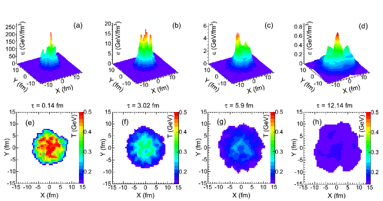
Figure 1: (Color online). Distributions of energy density (upper panles) and temperature (lower panels) in the transverse ($X$-$Y$) plane at four proper times ($\tau$), obtained from hydrodynamic calculations for one central Pb-Pb event at $\sqrt{{s_{\rm NN}}}$ =2.76 TeV.

Recent experimental data from the Relativistic Heavy Ion Collider (RHIC) and the Large Hadron Collider (LHC) have confirmed the formation of a strongly coupled system. Hydrodynamics has been used extensively and to a large extent successfully to explain majority of these experimental results song . A (2+1)-dimensional event-by-event ideal hydrodynamical framework hannu is used in the present work to model the space-time evolution of the system produced in most central (0–5% of the total cross section) collisions of lead nuclei at $\sqrt{{s_{\rm NN}}}$ = 2.76 TeV at LHC. A lattice-based equation of state eos is used in this model and 170 MeV is considered as the transition temperature from the QGP to a hadronic phase. This model has been successfully used to explain the spectra and elliptic flow of hadrons at RHIC and LHC energies hannu . In this Monte Carlo Glauber model, the standard two-parameter Woods-Saxon nuclear density profile is used to distribute the nucleons randomly into the colliding nucleons. Two nucleons from different nuclei are assumed to collide when $d^{2}<\sigma_{\rm NN}/\pi$, where $d$ is the transverse distance between the nuclei and $\sigma_{\rm NN}$ is the inelastic nucleon-nucleon cross section. For LHC energies, we take $\sigma_{\rm NN}=64$ mb and the initial formation time of the plasma $\tau_{0}=$ 0.14 fm phe ; hannu ; chre1 . A wounded nucleon (WN) profile is considered where the initial entropy density is distributed around the WN using a 2-dimensional Gaussian distribution function,

$$s(X,Y)=\frac{K}{2\pi\sigma^{2}}\sum_{i=1}^{\ N_{\rm WN}}\exp\Big{(}-\frac{(X-X_{i})^{2}+(Y-Y_{i})^{2}}{2\sigma^{2}}\Big{)}.$$ (1)

Here $X_{i},Y_{i}$ are the transverse coordinates of the $i^{\rm th}$ nucleon and $K$ is an overall normalization constant. The size of the density fluctuations is determined by the free parameter $\sigma$, which is taken to be 0.4 fm hannu . The temperature at freeze-out is taken as 160 MeV, which reproduces the measured $p_{\rm{T}}$ spectra of charged pions at LHC.

Figure 1 shows the distributions of $\epsilon$ and $T$ for a single event in $X$-$Y$ bins (each bin is of size 0.6 fm$\times$0.6 fm) at four different values of proper time ($\tau$). The upper panels (a-d) show a three dimensional view of $\epsilon$, whereas the lower panels (e-h) show the $T$ variations in the transverse plane. At early times, sharp and pronounced peaks in $\epsilon$ and hotspots in $T$ are observed. These bin-to-bin fluctuations in $\epsilon$ and $T$ indicate that the system formed immediately after collision is inhomogeneous in phase space and quite violent. As time elapses, the system cools, expands, and the bin-to-bin variations in $\epsilon$ and $T$ smoothens out tending towards a homogenous system at freeze-out.

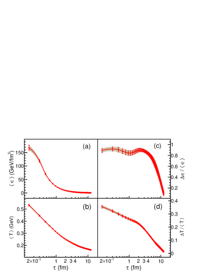
Figure 2: (Color online). Temporal evolution of (a) average energy density, (b) average temperature, (c) fluctuations in energy density, and (d) fluctuations in temperature, for central Pb-Pb collisions at $\sqrt{{s_{\rm NN}}}$ =2.76 TeV, obtained from hydrodynamic calculations. The shaded regions represent the extent of event-by-event variations.

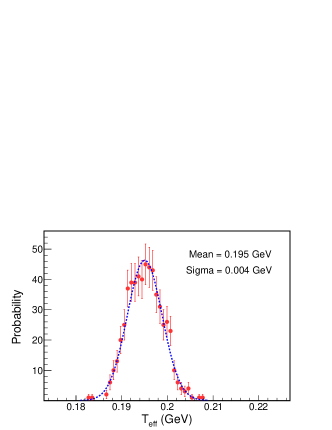
Figure 3: (Color online). Bin-to-bin distribution of $T_{\rm eff}$ of pions for 16$\times$36 bins in $y$–$\phi$ for central Pb-Pb collisions at $\sqrt{{s_{\rm NN}}}$ = 2.76 TeV using the AMPT model.

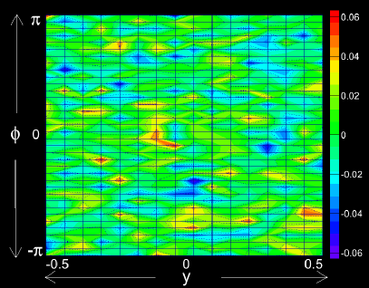
Figure 4: (Color online). Temperature fluctuation map in $y$–$\phi$ phase space for central (0–5%) Pb-Pb collisions at $\sqrt{{s_{\rm NN}}}$ = 2.76 TeV using the AMPT model. The right hand color palettes show the magnitude of fluctuations.

Observations from Fig. 1 can be quantified by studying the mean energy density ($\langle\epsilon\rangle$), mean temperature ($\langle T\rangle$) over all the bins, and the bin-to-bin fluctuations of $\epsilon$ and $T$ at each $\tau$. Figure 2 presents the time evolution of $\langle\epsilon\rangle$ and $\langle T\rangle$, and their fluctuations. The $x$-axes are plotted in logarithmic scale for zooming in on the early times. The event-by-event variations of these quantities are represented by the shaded regions, taken from about 500 events. The $\langle\epsilon\rangle$ and $\langle T\rangle$ decrease as time elapses. The value of $\langle\epsilon\rangle$ falls sharply from $\sim$168 GeV/fm³ at $\tau=0.14$ fm to a value of $\sim$20 GeV/fm³ at $\tau=1$ fm, and then falls slowly till freeze-out. The initial energy density valus are close to the results from the ALICE collaboration, $\epsilon$$\tau$$\sim$16 GeV/fm² alice_energy . On the other hand, the fall of $\langle T\rangle$ with $\tau$ is smooth, which goes down from $\sim$530 MeV at $\tau=0.14$ fm to $\sim$300 MeV at $\tau=1$ fm. At the freeze-out, $\langle T\rangle$ is close to 160 MeV.

The bin-to-bin fluctuations in $\epsilon$ and $T$ have been quantified by $\Delta\epsilon/\langle\epsilon\rangle$ and $\Delta T/\langle T\rangle$, where $\Delta\epsilon$ and $\Delta T$ are the root mean square (RMS) deviations. Time evolutions of fluctuations in $\epsilon$ and $T$ are presented in the right panels of Fig. 2. Extremely large fluctuations in energy density of $\sim$90% are observed at early times, confirming the violent nature of the collision. At the same time, the fluctuations in $T$ are smaller ($\sim$35%). Interestingly, although $\langle\epsilon\rangle$ decreases quite fast, the fluctuation in $\epsilon$ remains almost constant up to $\tau$$\sim$2.5 fm, then falls rapidly. Around the same value of $\tau$, the fluctuation in $T$ shows a kink, where the change in fluctuation increases. There may be a characteristic change in the behaviour of the system at this $\tau$ during the hydrodynamic evolution. A close analysis of the time evolution of different phases indicates that these changes in nature of the fluctuations happen at a time when the hadronic phase starts to dominate over the QGP phase.

Fluctuation measurements in heavy-ion experiments are possible only at freeze-out. The connection from the freeze-out to the early stages of colision can be made by comparing experimental data with theoretical calculations at freeze-out. For this comparison, the available phase space of experimental data is divided into bins of $y$-$\phi$. For each bin, the $p_{\rm{T}}$ spectrum of identified particles can be constructed, from which one can extract the effective temperature ($T_{\rm eff}$). The bin-to-bin fluctuation of $T_{\rm eff}$ are used to construct fluctuation maps and attempt to make a connection to the hydrodynamic calculations. The applicability of this method is demonstrated below using the AMPT event generator.

We employ the string melting (SM) mode of the AMPT model ampt to mimic the experimental conditions for Pb-Pb collisions at $\sqrt{{s_{\rm NN}}}$ = 2.76 TeV. This mode includes a fully partonic QGP phase that hadronizes through quark coalescence, and has been shown to reproduce the experimental data at LHC energies subrata ; cmko1 ; cmko2 ; dronika . The parameter set-B as discussed in cmko1 ; cmko2 is used for the event generation. We choose events with 0–5% centrality window to ensure that the event-to-event variation in the number of participating nucleons is minimal.

The phase space around the central rapidity ($-0.5\leq y\leq 0.5$) and full azimuth ($-\pi\leq\phi\leq\pi$) is divided into a number of bins in $y$–$\phi$. We present results of the calculation with a grid of 16$\times$36 bins, where the bin sizes are well within the detector resolutions for the present experiments at RHIC and LHC. The $p_{\rm{T}}$ spectrum of charged pions are constructed for each $y$–$\phi$ bin by combining a large number of events. For each of the bins, the $p_{\rm{T}}$ spectrum is fitted by a Maxwell-Boltzmann function within $0.5\leq p_{\rm T}\leq 1.0$ GeV to obtain $T_{\rm eff}$. This $p_{\rm{T}}$ range is chosen to exclude very low $p_{\rm{T}}$ pions coming from resonance decays and high $p_{\rm{T}}$ pions affected by mini-jets alice . $T_{\rm eff}$ has contributions from two components, a thermal part and a second part which depends on the collective transverse velocity ($\langle\beta_{\rm T}\rangle$) of the system. Assuming that the second component is similar for all the events within a narrow centrality event class, the fluctuation in $T_{\rm eff}$ can be considered to be a good representation of the fluctuation in kinetic temperature. Figure 3 shows the distribution of $T_{\rm eff}$ for all the bins, fitted with a Gaussian distribution. The mean and the sigma of the distribution are 195 MeV and 3.8 MeV respectively, which represents a fluctuation of 2% over all the bins.

We construct the fluctuation map in $y$–$\phi$ bins, where the temperature fluctuation in each bin is calculated in terms of $\Delta T_{\rm eff}/\langle T_{\rm eff}\rangle$, where $\Delta T_{\rm eff}=(\langle T_{\rm eff}\rangle-T_{\rm eff})$. Here $T_{\rm eff}$ is the effective temperature of a particular bin and $\langle T_{\rm eff}\rangle$ is the average value over all bins. Figure 4 shows the fluctuation map for all the $y$–$\phi$ bins and the amount of fluctuations from the mean value is represented by different colors. The color palettes are smeared in the profile histogram for a better representative view.

The map gives a quantitative view of the temperature fluctuations in the available phase space. It clearly shows several hot (red) as well as cold (blue) spots, with average (green) zones throughout the phase space. These spots may have their origin from the extreme regions of phase space, which existed during the early stages of the reaction. This may indicate that the observed fluctuations are remnants of the initial energy density fluctuations and are not washed out until the freeze-out stage. The amount of these fluctuations are similar to those from hydrodynamic calculations at $\tau\sim$12 fm. Thus, within the present theoretical framework, we can make a correspondence to the early stage of the collision through the hydro calculations. Furthermore, these fluctuation maps can form the basis of power spectrum analysis ajit ; paul ; morphology .

In CMBR studies of the Big Bang, there is only one event, whereas in the case of heavy-ion collision experiments, one has access to very large number of events. This can be used as an advantage in order to gain access to the primordial state. Event-by-event fluctuations are sensitive to the changes in the state of the matter, and give additional thermodynamic information. Event-by-event temperature fluctuations are related to the heat capacity ($C_{\rm v}$) of the system Sto ; korus ; steph ; gavai-gupta ; wilk ; shuryak ; morw :

$$C_{\rm v}^{-1}=(\Delta T^{\rm ebye}_{\rm eff}/\langle T^{\rm ebye}_{\rm eff}\rangle)^{2},$$ (2)

where $T^{\rm ebye}_{\rm eff}$ is the effective temperature, obtained on an event-by-event basis. At LHC energies, central Pb-Pb collisions produce a large number of particles in each event, which makes the event-by-event analysis of several observables within the reach of the experiments. We have constructed $p_{\rm{T}}$ distributions of charged pions on an event-by-event basis for a large number of AMPT events corresponding to 0-5% centrality. The $p_{\rm{T}}$ spectrum for each event is fitted with Maxwell-Boltzmann function to obtain $T^{\rm ebye}_{\rm eff}$. The distribution of $T^{\rm ebye}_{\rm eff}$, fitted with a Gaussian distribution, is shown in Fig. 5, which gives the mean and sigma as 182 MeV and 15 MeV respectively, which yields $C_{\rm v}=147$ for the system at freeze-out. This method opens up a new avenue for accessing the thermodynamic parameters.

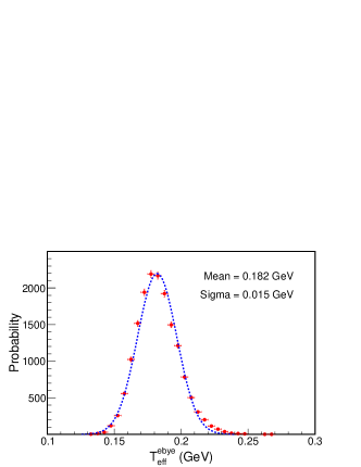
Figure 5: (Color online). Event-by-event distribution of $T^{\rm ebye}_{\rm eff}$ for pions within central rapidity and full azimuth for central Pb-Pb collisions at $\sqrt{{s_{\rm NN}}}$ = 2.76 TeV using AMPT model.

We discuss the following effects which can affect temperature fluctuations:

Mean $p_{\rm{T}}$: Similar fluctuation maps may be constructed from fluctuation of mean transverse momentum ($\langle p_{\rm T}\rangle$) of charged particle spectra na49 . However, $\langle p_{\rm T}\rangle$ may not be a good measure of the temperature steph .

Event plane orientation: Event plane orientation is necessary for studying bin-to-bin fluctuations, especially for non-central collisions. For the present study, AMPT events are event plane oriented.

Flow effect: Fourier decomposition of the momentum distribution in transverse plane yields a $\phi$–independent, axially symmetric radial flow component and a $\phi$–dependent part containing the anisotropic flow coefficients. For most central collisions within a narrow centrality bin, radial flow remains similar for all the events and the anisotropic flow components do not affect the slope of the $p_{\rm{T}}$ distribution.

Final state effects: Final state effects, such as resonance decay, and hadronic rescattering tend to make the $p_{\rm{T}}$ spectra softer, mostly below 0.5 GeV. To mitigate this effect, the fit range is chosen to be 0.5 GeV to 1.0 GeV.

Finite multiplicity effect: Pb-Pb collisions at LHC energies produce a large number of particles which are adequate for event-by-event studies. The number bins in constructing the map should not be too large in order to avoid the empty bin effect.

Number of $y$–$\phi$ bins: The limitation of choosing the number of bins is constrained by detector resolutions of the various experiments. This is tested the by choosing several $y$–$\phi$ bins (16$\times$16, 16$\times$24 and 16$\times$36). The bin-to-bin temperature fluctuations remain within 1.3% to 2%.

Event averaging: Temperature fluctuation map involves constructing the $p_{\rm{T}}$ spectrum in a given $y$–$\phi$ bin by including particles from a large number of events. As the final spectrum is event averaged, the averaging does not affect the determination of slope parameters.

Species dependence: As the particle production mechanism of baryons, mesons and strange particles are different, species dependence of temperature fluctuations may provide extra information of their freeze-out hyper-surfaces. Whether the origin of the temperature fluctuations are solely due to initial state fluctuations or any final state effect, this will be interesting to study in the species dependence of temperature fluctuations.

Viscosity effect: Viscosity tends to dilute the fluctuations. The SM version of AMPT includes the effect of viscosity ($\eta/s\sim 0.15$ at $T$=436 MeV subrata ; dronika ). Analysis using a viscous hydrodynamic model is in progress.

In conclusion, we have shown that temperature fluctuation maps, similar to those in CMBR experiments, offer a novel way of representing data in heavy-ion collisions. Experimentally, it is possible to obtain bin-to-bin fluctuations in temperature from the transverse momentum distributions in $y$–$\phi$ bins. Interestingly, quantitative similar fluctuations are obtained from hydrodynamic model calculations for most central Pb-Pb collisions at the LHC. Non-zero fluctuations imply that some of the signals of the initial state fluctuations remain as imprints at the freeze-out, this connection has been established within the framework of a hydrodynamic model. Important information like the speed of sound, specific heat, etc., can be extracted from event-by-event temperature fluctuations. We emphasize that this novel way of studying temperature fluctuations will open new avenues of studying heavy-ion collisions and will be useful in obtaining proper insight into the little bang and QGP matter.

We would like to thank H. Holopainen for providing us with the event-by-event hydrodynamic code. We gratefully acknowledge stimulating discussions with Satyajit Jena, Alexander Philipp Kalweit, Steffen Bass, Dinesh Srivastava, Sudhir Raniwala, Paolo Giubellino, Jurgen Schukraft, Zi-Wei Lin, Daniel McDonalds and Bikash Sinha.

References

- (1) E. Komatsu and C. L. Bennett (WMAP science team) arXiv:1404.5415 [astro-ph.CO].
- (2) A.I. Fisenko and V. Lemberg, arXiv:1401.1432 [astro-ph.CO].
- (3) P.A.R. Ade et al. (Planck Collaboration), arXiv:1303.5062 [astro-ph.CO].
- (4) W. Florkowski, Phenomenology of Ultra-relativistic Heavy-ion Collisions, World Scientific, 2010.
- (5) U. Heinz, J. Phys.: Conf. Ser. 455, 012044 (2013).
- (6) P. Naselsky et al. Phys. Rev. C 86, 024916 (2012).
- (7) A. Mocsy and P. Sorensen, Nucl. Phys. A 855, 241 (2011).
- (8) A.P. Mishra et al., Phys. Rev. C 77, 064902 (2008); ibid., Phys. Rev. C 81, 034903 (2010).
- (9) Z.-W. Lin, C.M. Ko, B.-A. Li, B. Zhang, S. Pal, Phys. Rev. C 72, 064901 (2005).
- (10) L. Stodolsky, Phys. Rev. Lett. 75, 1044 (1995).
- (11) R. Korus et al., Phys. Rev. C 64, 054908 (2001).
- (12) M.A. Stephanov, K. Rajagopal and E. V. Shuryak, Phys. Rev. D 60, 114028 (1999).
- (13) R. Gavai, S. Gupta and S. Mukherjee, Phys. Rev. D 71, 074013 (2005).
- (14) G. Wilk and Z. Wlodarczyk, Phys. Rev. Lett. 84, 2770 (2000).
- (15) E.V. Shuryak, Phys. Lett. B 423, 9 (1998).
- (16) S. Mrowczynski, Phys. Lett. B 430, 9 (1998).
- (17) H. Song, arXiv:1401.0079v1 [nucl-th].
- (18) H. Holopainen, H. Niemi, and K. Eskola, Phys. Rev. C 83, 034901 (2011).
- (19) M. Laine and Y. Schroder, Phys. Rev. D 73, 085009 (2006).
- (20) R. Chatterjee, H. Holopainen, T. Renk, and K. J. Eskola, Phys. Rev. C 83, 054908 (2011).
- (21) R. Paatelainen, K.J. Eskola, H. Holopainen, and K. Tuominen, Phys. Rev. C 87, 044904 (2013).
- (22) K. Aamodt et al., (ALICE Collaboration), Phys. Rev. Lett. 105, 252301 (2010); A. Toia (ALICE Collaboration), Jour. Phys. G 38, 124007 (2011).
- (23) S. Pal and M. Bleicher, Phys. Lett. B 709, 82 (2012).
- (24) J. Xu and C.M. Ko, Phys. Rev. C 83, 034904 (2011).
- (25) J. Xu and C.M. Ko, Phys. Rev. C 84, 014903 (2011).
- (26) D. Solanki, P. Sorensen, S. Basu, R. Raniwala, T.K. Nayak, Phys. Lett. B 720, 352 (2013).
- (27) B. Abelev et al. (ALICE Collaboration), Phys. Rev. Lett. 109, 252301 (2012).
- (28) H. Appelshauser et al. (NA49 Collaboration), Phys. Lett. B 459, 679 (1999).