VARIATIONAL METHOD
FOR THE CALCULATION OF CRITICAL DISTANCE
BETWEEN TWO COULOMB CENTERS IN GRAPHENE

Abstract

The supercritical instability in a system of two identical charged impurities in gapped graphene described in the continuous limit by the two-dimensional Dirac equation has been studied.  The case where the charge of each impurity is subcritical, but their sum exceeds the critical value calculated in the version with a single Coulomb center, is considered.  Using the developed variational method, the dependence of the critical distance $R_{\rm cr}$ between the impurities on their total charge is calculated.  The $R_{\rm cr}$-value is found to grow as the total impurity charge increases and the quasiparticle band gap decreases.  The results of calculations are compared with those obtained in earlier researches.

1 Introduction

The gapless linear spectrum of graphene was determined rather long ago [1], while constructing the band model of graphite provided that the interaction between the planes of carbon atoms is neglected.  Nevertheless, graphene itself was obtained for the first time only in 2004 [2], which launched its intense theoretical and experimental study.  Graphene permanently attracts attention of scientists throughout the world owing to its unique properties.  In particular, it is one of the first two-dimensional crystals and possesses the ultrahigh mechanical strength and the charge carrier mobility, which determines the prospects of its application in novel nanoelectronics.  The physics of graphene is also of interest from the viewpoint of fundamental scientific researches, because it turned out to have a deep relation to quantum electrodynamics (QED) and other quantum field theories.

Graphene has a honeycomb crystalline lattice.  In the tight-binding approximation, the spectrum of low-energy quasiparticle excitations is linear, and the latter are described by a $2+1$-dimensional massless Dirac equation [3,​ 4,​ 5,​ 6].  Hence, in the continuous limit, we obtain an effective quantum field theory with $2+1$-dimensional Dirac fermions that interact with the ordinary three-dimensional Coulomb potential, $\sim 1/r$.  Those circumstances testify to a capability of the solid-state implementation of experiments aimed at detecting such QED phenomena as the Klein paradox, Schwinger effect (the creation of pairs in a strong external electric field), supercritical atomic collapse, and others, which have not yet been observed in the Nature.  The Klein tunneling was really revealed in graphene [7], and the supercritical atomic collapse of charged impurities was recently observed experimentally [8].

The solution of the relativistic Kepler problem with regard for the finite size of an atomic nucleus [9] showed that, if the so-called critical charge of a nucleus, $Z_{\mathrm{cr}}\approx 170$, is exceeded, the energy levels of bound states dives into the lower continuum, and the escape of positrons is observed [11,​ 10].  However, there are no nuclei with this charge, and, hence, the effect has not been observed.  Somewhat later, there emerged an idea concerning head-on (or almost head-on) collisions between the nuclei of heavy atoms, e.g., uraniums [12,​ 13,​ 14,​ 10].  In this case, the total charge of the nuclei exceeds the critical value, and there exists a distance between the nuclei, at which the lowest bound state dives into the lower continuum.  This distance is also called critical.  Unfortunately, in the relativistic problem of two centers, the variables cannot be separated in any coordinate system, so that an analytical solution cannot be derived [11,​ 10].  However, the calculations with the help of approximate quantum-mechanical methods, in particular, the variational one [15], were carried out, and the dependences of the critical distance between the nuclei on the total system charge were plotted.

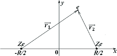
Fig. 1.: Electron in the field of two Coulomb impurities

In the physics of graphene, the Fermi velocity, $v_{\mathrm{F}}\approx 10^{6}\leavevmode\nobreak\ \mathrm{m/s}$, appears instead of the light velocity $c$.  As a result, the “fine structure constant” for graphene is $\alpha=\frac{e^{2}}{\hbar v_{\mathrm{F}}}\approx 2.19$.  However, graphene is actually located on a dielectric substrate.  Therefore, the interaction with an impurity with charge $Ze$ is described by the constant $\beta=Z\alpha/\kappa$, where $\kappa$ is the dielectric permittivity of a substrate.  The problem of supercritical instability of a single charged impurity in gapless graphene was studied in detail in works [16,​ 17].  In the case of graphene with the gap $2\Delta$ and the regularized Coulomb potential $V(r)=-\frac{Ze^{2}}{\kappa r}\theta(r-R)-$ $-\frac{Ze^{2}}{\kappa R}\theta(R-r)$, the transition to the supercritical mode was found to occur at $\beta_{\mathrm{c}}=1/2+\pi^{2}/\log^{2}(c\Delta R/\hbar v_{\mathrm{F}})$, where $c\approx 0.21$.

Although the supercritical instability manifests itself in graphene already at impurity charges $Z\gtrsim 1$, a possibility to detect it is illusory because of experimental difficulties associated with the production of impurities, whose charge is larger than 1.  The solution of this task consists in arranging a few charged impurities on a small section of graphene.  Just this approach was implemented by a group of scientists from the University of California [8], while observing the supercritical instability in graphene (ionized dimers of calcium were used as impurities).  Hence, despite that the coupling constant in graphene is larger by a factor of 300, the necessity to consider a few, rather than one, impurities located closely to one another arises in this case as well, the configuration with two Coulomb centers being the simplest variant.  In work [19], the critical distance between impurities was calculated, and the position and the width of a resonance that arises in the lower continuum in the supercritical mode were determined in the first approximation with the use of variational technique.

This work aims at obtaining the next (second) approximation in the framework of the variational method.  The article structure is as follows.  In Section 2, the problem is formulated, and the asymptotics for the wave function of a state that dives into the lower continuum are determined.  The variational method to find the critical distance between impurities is described in Section 3.  In Section 4, the results obtained are discussed, and some conclusions are made.

2 Statement of the Problem

In the tight-binding approximation, the band spectrum of graphene has a valence band and a conduction band that touch each other at two nonequivalent points of the reciprocal crystalline lattice.  These are the so-called Dirac points ${\bf K}_{\pm}$.  The spectrum of low-energy excitations is linear.  The effective Hamiltonian that describes electron quasiparticle excitations in vicinities of the Dirac points has the form of a $2+1$-dimensional Dirac Hamiltonian.  In the case where there is a quasiparticle gap between the valence and conduction bands, the Hamiltonian also includes the mass term

$$H=v_{\mathrm{F}}\bm{\tau}\bm{p}+\xi\Delta\tau_{z}+V(r),$$ (1)

where $\bm{p}$ is the canonical momentum, $\tau_{i}$ are the Pauli matrices, and $\Delta$ is the quasiparticle gap halfwidth.  This Hamiltonian operates in the space of two-component spinors $\Psi_{\xi s}$ distinguished by the valley ($\xi=\pm$) and spin ($s=\pm$) subscripts.  It is generally adopted that $\Psi_{+s}^{T}=(\psi_{A},\psi_{B})_{K_{+}s}$ and $\Psi_{-s}^{T}=$ $=(\psi_{B},\psi_{A})_{K_{-}s}$, where $A$ and $B$ are the corresponding sublattices of the hexagonal lattice in graphene. The interaction potential reads

$$V\left(\mathbf{r}\right)=-\frac{e^{2}}{\kappa}\left(\!\frac{Z_{1}}{r_{1}}+\frac{Z_{2}}{r_{2}}\!\right)\!,$$ (2)

where $\kappa$ is the dielectric permittivity of the substrate, $Z_{1,2}$ are the impurity charges, and $r_{1,2}=|\mathbf{r}\pm\mathbf{R}/2|$ are the distances reckoned from the Coulomb impurities to the electron (see Fig. 1).  The potential does not depend on the spin, so that we will omit the spin subscript below.  We also suppose that the electron is located near the Dirac point $\bm{K}_{+}$.  If the electron is located near the point $\bm{K}_{\_}$, $\Delta$ has to be substituted by $-\Delta$ everywhere.  In recent experiments [8], identical impurities were considered, and we also put $Z_{1}=$ $=Z_{2}=Z$ in this work.

Hence, the Dirac equation for an electron in the potential of two charged impurities looks like

$$\left(v_{\rm F}\tau_{x}p_{x}+v_{\rm F}\tau_{y}p_{y}+\Delta\tau_{z}+V\left(\mathbf{r}\right)\right)\Psi(\mathbf{r})=E\Psi(\mathbf{r}).$$ (3)

For the two-component spinor $\Psi(\mathbf{r})=(\phi,\chi)^{T}$, it can be rewritten in the form

$$\left\{\!\!\!\begin{array}[]{l}\displaystyle\left(E-V-\Delta\right)\phi+iv_{\rm F}\left(\!\frac{\partial}{\partial x}-i\frac{\partial}{\partial y}\!\right)\chi=0,\\[8.53581pt] \displaystyle\left(E-V+\Delta\right)\chi+iv_{\rm F}\left(\!\frac{\partial}{\partial x}+i\frac{\partial}{\partial y}\!\right)\phi=0.\end{array}\right.$$ (4)

Expressing the component $\chi$ from the second equation of system (4) and substituting it to the first one, we obtain the following second-order differential equation for the spinor component $\phi$:

$$(\partial^{2}_{x}+\partial^{2}_{y})\phi+\frac{\frac{\partial V}{\partial x}-i\frac{\partial V}{\partial y}}{E-V+\Delta}\left(\!\frac{\partial\phi}{\partial x}+i\frac{\partial\phi}{\partial y}\!\right)+$$

$$+\,v^{-2}_{\rm F}\left((E-V)^{2}-\Delta^{2}\right)\phi=0.$$ (5)

The supercritical instability takes place when the lowest bound state dives into the lower continuum, i.e.  when $E=-\Delta$ [10,​ 11].  In the further calculations, only this energy value will be considered.

2.1 Asymptotic behavior of the wave function

Let us analyze the asymptotic behavior of the wave function at large distances, $r\rightarrow\infty$.  In this limit, the potential looks like

$$V\left(\mathbf{r}\right)=-\zeta v_{\rm F}\left(\!\frac{1}{r}+\frac{R^{2}}{4r^{3}}P_{2}(\cos\varphi)+O\left(\!\frac{1}{r^{5}}\!\right)\!\right)\!,$$ (6)

where $\zeta=2Z\alpha/\kappa$, and $P_{2}(x)$ is the Legendre polynomial of the second order.  Substituting potential (6) into Eq. (5) and preserving only the most contributing terms, we obtain

$$\phi^{\prime\prime}+\frac{2}{r}\phi^{\prime}+\left(\!\frac{\zeta^{2}}{r^{2}}-\frac{2m\zeta}{r}\!\right)\phi=0,$$ (7)

where $m=\Delta/v_{\mathrm{F}}$ is the inverse Compton wavelength of quasiparticles.  The solution of this equation vanishing at infinity is described by the Macdonald function as follows:

$$\phi(r)=Cr^{-1/2}K_{i\gamma}(\sqrt{8m\zeta r}),\quad\gamma=\sqrt{4\zeta^{2}-1}.$$ (8)

Then, with regard for the asymptotic behavior of the Macdonald function [20], we have

$$\phi_{\mathrm{asym}}(r)=\tilde{C}r^{-3/4}\exp(-\sqrt{8m\zeta r}),\quad r\rightarrow\infty.$$ (9)

To study the asymptotic behavior of the solution in a vicinity of either of the impurities, it is convenient to change to the elliptic coordinate system ($\xi$, $\eta$), where

$$\xi\equiv\frac{r_{1}+r_{2}}{R},\leavevmode\nobreak\ \leavevmode\nobreak\ \leavevmode\nobreak\ \leavevmode\nobreak\ \leavevmode\nobreak\ \eta\equiv\frac{r_{1}-r_{2}}{R}.$$ (10)

The new coordinates can be varied within the intervals

$$1\leq\xi<\infty,\leavevmode\nobreak\ \leavevmode\nobreak\ \leavevmode\nobreak\ \leavevmode\nobreak\ \leavevmode\nobreak\ -1\leq\eta\leq 1,$$

and the impurities are located at the points $(\xi=1,$ $\eta=\pm 1)$.

In the elliptic coordinates, the interaction potential looks like

$$V\left({\bf r}\right)=-\frac{2\zeta v_{\mathrm{F}}\xi}{R(\xi^{2}-\eta^{2})}.$$ (11)

In a vicinity of either of the impurities, the quantity $\xi^{2}-\eta^{2}$ is small. In the elliptic coordinates, Eq. (5) reads

$$\frac{4}{R^{2}\left(\xi^{2}-\eta^{2}\right)}\biggl{[}\sqrt{\xi^{2}-1}\frac{\partial}{\partial\xi}\left(\!\sqrt{\xi^{2}-1}\frac{\partial}{\partial\xi}\!\right)+$$

$$+\,\sqrt{1-\eta^{2}}\frac{\partial}{\partial\eta}\left(\sqrt{1-\eta^{2}}\frac{\partial}{\partial\eta}\right)\!\biggr{]}\phi\,+$$

$$+\,\frac{4}{R^{2}\xi(\xi^{2}-\eta^{2})^{3}}\biggl{[}\xi^{4}\eta+3\xi^{2}\eta^{3}-3\xi^{2}\eta-\eta^{3}\,-$$

$$-\,i\sqrt{(\xi^{2}-1)(1-\eta^{2})}(\xi^{3}+3\xi\eta^{2})\!\biggr{]}\times$$

$$\times\biggl{[}\!\left(\eta(\xi^{2}-1)+i\xi\sqrt{(\xi^{2}-1)(1-\eta^{2})}\right)\frac{\partial\phi}{\partial\xi}\,+$$

$$+\left(\xi(1-\eta^{2})-i\eta\sqrt{(\xi^{2}-1)(1-\eta^{2})}\right)\frac{\partial\phi}{\partial\eta}\biggr{]}+$$

$$+\left(\!\frac{4\zeta^{2}\xi^{2}}{R^{2}(\xi^{2}-\eta^{2})^{2}}-\frac{4\zeta m\xi}{R(\xi^{2}-\eta^{2})}\!\right)\phi=0.$$ (12)

We seek a solution in the form $\phi(\xi,\eta)=\phi(\mu)$, where $\mu=\xi^{2}-\eta^{2}=4r_{1}r_{2}/R^{2}$.  After the substitution in Eq.  (12), we retain only the most weighty terms and obtain the equation

$$\frac{d^{2}\phi}{d\mu^{2}}+\frac{2}{\mu}\frac{d\phi}{d\mu}+\frac{\zeta^{2}}{4\mu^{2}}\phi=0,$$ (13)

whose solution regular as $\mu\to 0$ is

$$\phi_{\mathrm{imp}}(\mu)=C_{2}\mu^{-\sigma/2},\quad\sigma=1-\sqrt{1-\zeta^{2}}.$$ (14)

Taking into account that $\mu\simeq 4r^{2}/R^{2}$ as $r\rightarrow\infty$, solution (8) can be rewritten in the form

$$\phi(\mu)=C_{1}\mu^{-1/4}K_{i\gamma}(2\sqrt{m\zeta R}\mu^{1/4}).$$ (15)

Matching solutions (14) and (15) across the point $\mu=1$, we obtain an implicit equation for the dependence of the critical distance $R_{\mathrm{cr}}$ on $\zeta$, namely, the transcendental equation

$$2\sqrt{1-\zeta^{2}}-1=2\sqrt{m\zeta R}\frac{K_{i\gamma}^{\prime}(2\sqrt{m\zeta R})}{K_{i\gamma}(2\sqrt{m\zeta R})}.$$ (16)

Its numerical solution is shown by the dash-dotted curve in Fig. 2.  In the next section, this dependence will be calculated more accurately with the help of the variational method.

3 Variational Method

As was indicated above, the relativistic Dirac equation, if being applied to the problem of two Coulomb centers, does not allow the variables to be separated in any orthogonal coordinate system; that is why it is impossible to obtain its solution in the analytical form.  While constructing an approximate solution, let us take advantage of the variational method, as was done in the case of QED [15].  In work [21], it was indicated that the highest accuracy within the variational method is achieved when the corresponding trial functions satisfy the asymptotics of the exact solution in vicinities of charged impurities and at infinity. Those asymptotics were obtained in the previous section.

In order to formulate the variational problem, it is enough to mark that the differential equation (5) can be derived, while analyzing the following functional with respect to the extremum value:

$$S[\phi]=\int\biggl{(}\!(E-V+\Delta)^{-1}\left|\frac{\partial\phi}{\partial x}+i\frac{\partial\phi}{\partial y}\right|^{2}-$$

$$-\,v^{-2}_{\rm F}(E-V-\Delta)|\phi|^{2}\!\biggr{)}dxdy,$$ (17)

and providing the norm preservation condition,

$$N=\int\Psi^{*}\Psi dxdy=\int\Biggl{[}v_{\rm F}^{-2}|\phi|^{2}\,+$$

$$+\,(E-V+\Delta)^{-2}\left|\frac{\partial\phi}{\partial x}+i\frac{\partial\phi}{\partial y}\right|^{2}\Biggr{]}dxdy.$$ (18)

Let us designate the new field as $\psi=W^{-1/2}\phi$, where $W=E-V+\Delta$.  Then the functional $S[\phi]$ can be expressed in the form typical of non-relativistic quantum mechanics,

$$S[\psi]=\int\biggl{[}|\bm{\nabla}\psi|^{2}+i\left(\!\frac{\bm{\nabla}V}{2W}\times\bm{\nabla}\psi^{*}\!\right)\psi\,-$$

$$-\,i\psi^{*}\left(\!\frac{\bm{\nabla}V}{2W}\times\bm{\nabla}\psi\!\right)+2(U-\epsilon)|\psi|^{2}\biggr{]}dxdy,$$ (19)

where $\mathbf{a}\times\mathbf{b}=\epsilon_{ij}a_{i}b_{j}$, $\epsilon=(E^{2}-\Delta^{2})/2v_{\mathrm{F}}^{2}$ is the effective energy, and the effective potential $U$ looks like

$$U=\frac{EV}{v_{\mathrm{F}}^{2}}-\frac{V^{2}}{2v_{\mathrm{F}}^{2}}+\frac{\triangle V}{4W}+\frac{3}{8}\frac{(\bm{\nabla}V)^{2}}{W^{2}}.$$ (20)

The second and third terms in functional (19) describe the pseudospin-orbit coupling.  The norm reads

$$N=\int\Biggl{[}|\bm{\nabla}\psi|^{2}\,+$$

$$+\,i\left(\!\frac{\bm{\nabla}V}{2W}\times\bm{\nabla}\psi^{*}\!\right)\psi-i\psi^{*}\left(\!\frac{\bm{\nabla}V}{2W}\times\bm{\nabla}\psi\!\right)+$$

$$+\left(\!\frac{W^{2}}{v_{\rm F}^{2}}+\frac{\triangle V}{2W}+\frac{5(\bm{\nabla}V)^{2}}{4W^{2}}\!\right)|\psi|^{2}\Biggr{]}W^{-1}dxdy,$$ (21)

being important if proper boundary conditions are selected.  In what follows, we are interested in the case where the lowest bound state dives into the lower continuum.  Therefore, we put $E=-\Delta$ ($\epsilon=0$) and $W=-V$.  As a result, the functional $S[\psi]$ becomes simpler.

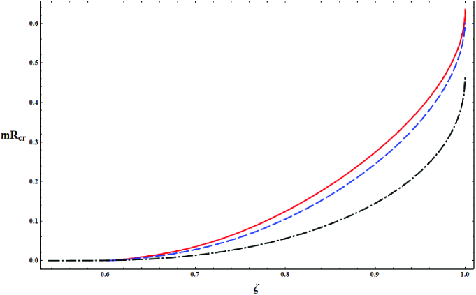
Fig. 2.: Dependences $mR_{\mathrm{cr}}(\zeta)$ obtained as numerical solutions of Eqs. (16) (dash-dotted curve) and (35) (solid curve).  For comparison, the results of calculations obtained in the first approximation of the variational method and taken from work [19] are exhibited by the dashed curve

In Section 2, the exact solution of the problem was found to depend only on the single variable $\mu$ in both asymptotic cases (14) and (15).  Therefore, we use the Kantorovich variational method (for more details, see Section 3 in review [22]) and select the sums

$$\psi=\sum\limits_{k=1}^{N}\psi_{k}(\mu)\nu^{k-1}$$ (22)

as trial functions.  Here, $\psi_{k}(\mu)$ compose a set of sought functions, and $\nu=\nu(\xi,\eta)$ is a fixed function of the coordinates, which is independent of $\mu$.  In work [15], two variants of the function $\nu$ were considered.  The results obtained turned out close enough.  Therefore, in this work, we select the variant $\nu=\eta^{2}/(\xi^{2}-\eta^{2})=$ $=(r_{1}-r_{2})^{2}/4r_{1}r_{2}$.

Substituting expression (22) into functional (19) and integrating over $\nu$, we obtain

$$S_{N}(\psi)=4\sum\limits_{k,l=1}^{N}\int\limits_{0}^{\infty}d\mu\biggl{(}\!P_{kl}\psi_{k}^{\prime}{\psi^{*}_{l}}^{\prime}+Q_{kl}\psi_{k}\psi^{*}_{l}+$$

$$+\,R_{kl}\psi_{k}^{\prime}\psi^{*}_{l}+R_{kl}^{\dagger}{\psi_{k}}{\psi^{*}_{l}}^{\prime}\!\biggr{)}\!,$$ (23)

where $\mathbf{\hat{P}}$, $\mathbf{\hat{Q}}$, and $\mathbf{\hat{R}}$ are $N\times N$-matrices depending on $\mu$.  The corresponding expressions for them are given in Appendix A (see Eqs. (A12)–(A14)).

Functional (23) reaches its minimum on the solutions of the Lagrange–Euler equations

$$\frac{d}{d\mu}\left(\!P_{kl}\frac{d\psi_{k}}{d\mu}+R_{kl}^{\dagger}\psi_{k}\!\right)-Q_{kl}\psi_{k}-R_{kl}\frac{d\psi_{k}}{d\mu}=0,$$ (24)

where $l=\overline{1,N}$.  The boundary conditions are so selected that the norm remains finite, and the trial functions satisfy the exact solution asymptotics.  The Lagrange–Euler equations and the corresponding boundary conditions constitute a boundary problem to be solved.

In work [19], the first approximation of the Kantorovich variational method with $N=1$ was used. The shooting method was used to calculate the dependence of the critical distance between two impurities on their total charge, $R_{\mathrm{cr}}(\zeta)$.  The result obtained is shown in Fig. 2 by the dashed curve for comparison.

A higher accuracy can be reached by applying the Kantorovich variational method with $N>1$. However, in this case, there are some differences from the case $N=1$ considered in work [19].  First of all, the shooting method is no more applicable, because the system of differential equations rather than a single equation is dealt with.  It was noticed in work [23], that, in order to simplify numerical calculations, the system of differential equations of the second order has to be reduced to a matrix differential equation of the first order with the use of the substitution

$$\psi_{i}^{\prime}(\mu)=\sum\limits_{j=1}^{N}Y_{ij}(\mu)\psi_{j}(\mu).$$ (25)

In this case, we obtain the following nonlinear matrix Riccati equation for the matrix $\mathbf{\hat{Y}}$:

$$\mathbf{\hat{Y}}^{\prime}=\mathbf{\hat{A}}-\mathbf{\hat{B}}\mathbf{\hat{Y}}-\mathbf{\hat{Y}}^{2}.$$ (26)

Here, the matrix coefficients $\mathbf{\hat{A}}$ and $\mathbf{\hat{B}}$ look like

$$\mathbf{\hat{A}}=\mathbf{\hat{P}}^{-1}(\mathbf{\hat{Q}}-\mathbf{\hat{R}}^{\prime}),$$ (27)

$$\mathbf{\hat{B}}=\mathbf{\hat{P}}^{-1}(\mathbf{\hat{R}}-\mathbf{\hat{R}}^{T}+\mathbf{\hat{P}}^{\prime}).$$ (28)

The matrices $\mathbf{\hat{P}}$, $\mathbf{\hat{Q}}$, and $\mathbf{\hat{R}}$ are singular at zero and infinity.  This is a reflection of the fact that the different functions $\psi_{k}(\mu)$, as well as different elements of the matrix $\mathbf{\hat{Y}}$, are characterized by different growth/fall degrees in vicinities of special points.  To overcome this inconvenience, let us subject the trial functions to a linear transformation,

$$\psi_{k}(\mu)=S_{kl}(\mu)\tilde{\psi}_{l}(\mu),\quad\det\mathbf{\hat{S}}(\mu)\neq 0.$$ (29)

The new matrix is designated as $\mathbf{\hat{Y}}_{\mathbf{S}}$,

$$\tilde{\psi}_{k}^{\prime}(\mu)=\left(Y_{\mathbf{S}}\right)_{kl}(\mu)\tilde{\psi}_{l}(\mu).$$ (30)

It is related to the matrix $\mathbf{\hat{Y}}$ by the formula

$$\mathbf{\hat{Y}}_{\mathbf{S}}=\mathbf{\hat{S}}^{-1}\mathbf{\hat{Y}}\mathbf{\hat{S}}-\mathbf{\hat{S}}^{-1}\mathbf{\hat{S}}^{\prime}.$$ (31)

The matrix $\mathbf{\hat{Y}}_{\mathbf{S}}$ also satisfies the Riccati equation,

$$\mathbf{\hat{Y}}_{\mathbf{S}}^{\prime}=\mathbf{\hat{A}}_{\mathbf{S}}-\mathbf{\hat{B}}_{\mathbf{S}}\mathbf{\hat{Y}}_{\mathbf{S}}-\mathbf{\hat{Y}}_{\mathbf{S}}^{2}.$$ (32)

The laws governing the change of coefficients in Eqs. (32) and (24) at transformation (29) are given in Appendix B.  They give rise to the criterion of choice of a matrix $\mathbf{\hat{S}}$; namely, the matrix $\mathbf{\hat{P}}_{\mathbf{S}}$ must be nondegenerate after the transformation, because the corresponding inverse matrix must exist as well.

In vicinities of each special points ($\mu=0$ and $\mu\rightarrow\infty$), the corresponding specific transformation matrix $\mathbf{\hat{S}}^{0/\infty}$ must be selected, and the transformed matrix coefficients $\mathbf{\hat{A}}_{\mathbf{S}}$ and $\mathbf{\hat{B}}_{\mathbf{S}}$ must be expanded in series in the variable $\mu$.  Accordingly, the sought matrix $\mathbf{\hat{Y}}_{\mathbf{S}}$ should be of the form

$$\begin{array}[]{l}\displaystyle\mathbf{\hat{Y}}_{\mathbf{S}}^{(0)}=\mu^{\lambda_{0}}\left(\!\mathbf{\hat{Y}}_{1}^{(0)}+\mu\mathbf{\hat{Y}}_{2}^{(0)}+\mu^{2}\mathbf{\hat{Y}}_{3}^{(0)}+...\!\right)\!,\ \mu\to 0,\\[8.53581pt] \displaystyle\mathbf{\hat{Y}}_{\mathbf{S}}^{(\infty)}\!=\!\mu^{\lambda_{\infty}}\left(\!\mathbf{\hat{Y}}_{1}^{(\infty)}\!+\!\frac{1}{\mu}\mathbf{\hat{Y}}_{2}^{(\infty)}\!+\!\frac{1}{\mu^{2}}\mathbf{\hat{Y}}_{3}^{(\infty)}\!+...\!\right)\!,\\[8.53581pt] \displaystyle\mu\to\infty.\end{array}\!\!\!\!\!\!\!\!\!\!$$ (33)

Let us substitute those formulas in Eq. (32) and equate the numerical coefficients of the terms with identical power exponents of the variable $\mu$.  We obtain a chain of coupled linear algebraic equations for the matrices $\mathbf{\hat{Y}}_{2}$, $\mathbf{\hat{Y}}_{3}$, and so on.  But, for the matrix $\mathbf{\hat{Y}}_{1},$ we have the quadratic equation

$$\mathbf{\hat{Y}}_{1}^{2}-\mathbf{\hat{B}}_{1}\mathbf{\hat{Y}}_{1}-\mathbf{\hat{A}}_{1}=0,$$ (34)

where $\mathbf{\hat{A}}_{1}$ and $\mathbf{\hat{B}}_{1}$ are some numerical matrices.  In the case where $N=2$, the transformation matrices can be selected to provide $\mathbf{\hat{B}}_{1}=B_{1}\mathbf{\hat{1}}$, and the quadratic matrix equation can be solved.  Of two roots, the root corresponding to a more regular behavior of the trial functions in vicinities of special points must be selected (namely, the positive root in a vicinity of $\mu=0$ and the negative one in a vicinity of $\mu\rightarrow\infty$).  The power exponents $\lambda_{0/\infty}$ are so selected to provide the coincidence of the power exponents in the most important terms on both sides of the equation.

In this way, the initial conditions for the matrix $\mathbf{\hat{Y}}_{\mathbf{S}}$ at zero and infinity were determined.  The corresponding matrices are presented in Appendix B.  Afterward, the Riccati equations were integrated numerically, by using the Runge–Kutta method and taking the initial conditions in the regions $\mu\in[0,1]$ and $\mu\in[1,\infty)$ into account.  Then the values of matrices $\mathbf{\hat{Y}}_{\mathbf{S}}^{0/\infty}(\mu=1)$ were calculated, and the inverse transformations were carried out to find the matrices $\mathbf{\hat{Y}}^{0/\infty}(\mu=1)$.  A smooth matching of trial functions in the intervals $\mu>1$ and $\mu<1$ can be done if

$$\delta(mR_{\mathrm{cr}},\zeta)\equiv\det[\mathbf{\hat{Y}}^{0}(\mu=1)-\mathbf{\hat{Y}}^{\infty}(\mu=1)]=0.\,\,$$ (35)

In this work, the case $N=2$ was considered.  The corresponding transformation matrices and the matrices of initial conditions are given in Appendix B.  All the actions described above were executed for various values of product $mR$ and at a fixed value of $\zeta$.  A value of $mR_{\mathrm{cr}}$, at which condition (35) was satisfied, was considered to be critical.  The results of numerical calculations were used to plot the dependence $mR_{\mathrm{cr}}(\zeta)$ (solid curve in Fig. 2).

4 Conclusions

A research of the supercritical instability in a system of two identical charged impurities in graphene is carried out.  The charge of each impurity is selected to be subcritical, but their sum $\zeta=2Z\alpha/\kappa$ exceeds the critical value $\zeta_{\mathrm{c}}=1/2$.  Hence, for every fixed $\zeta$, there exist a distance $R_{\mathrm{cr}}$ between the impurities, at which a supercritical regime is realized.  The urgency of the presented research is associated with recent observations of the supercritical instability in clusters of Ca impurities located on graphene [8].

The characteristic feature of this problem consists in that the variables in the Dirac equation cannot be separated in any known coordinate system.  Therefore, it is impossible to obtain the solution in the analytical form, and the Kantorovich variational method was applied to find the dependence of the critical distance on the charge of the system.  For massless particles, the critical phenomena are associated only with the emergence of a resonance in the lower continuum.  Since it is inconvenient to work with resonances within the variational method, a gap $\Delta$ was supposed to exist in the band spectrum of graphene.  Such a gap can be created experimentally by plenty of techniques, e.g., changing to a graphene nanoribbon, creating deformations, hydrogenating the surface, and so forth [24].  The presence of a gap results in the appearance of levels belonging to a discrete spectrum.  Therefore, a diving of the lowest level into the lower continuum is observed.  The distance between the impurities, at which this diving takes place, is called critical.

The Kantorovich variational method provides an opportunity for an arbitrary number of trial functions to be used.  In this work, a variant of the method with two trial functions was applied.  For the sake of comparison, the results of similar calculations but with only one trial function, which were carried out in work [19], are also presented.  The calculated dependences of $mR_{\mathrm{cr}}$ on $\zeta$, as well as the corresponding approximate curve obtained by matching the exact solution asymptotics, are plotted in Fig. 2.  One can see that the results of two consecutive approximations by the variational method agree rather well with each other both qualitatively and quantitatively.  The maximum discrepancy between them does not exceed $8\div 10\%$.  This fact testifies that, despite the simplicity of the applied approximation, the results obtained in work [19] are satisfactory: as it should be, $R_{\mathrm{cr}}\rightarrow 0$ as $\zeta\rightarrow 1/2$ (i.e.  the supercritical instability occurs only if the impurities are brought together) and $R_{\mathrm{cr}}\rightarrow\infty$ as $\zeta\rightarrow 1$ (i.e.  each impurity becomes supercritical). It is also demonstrated that, as $\Delta\rightarrow 0$, the value $R_{\mathrm{cr}}\rightarrow\infty$ for any fixed $\zeta$.  This means that, if the total charge in the system exceeds the critical one, the system is in the supercritical state at any finite distance between the impurities.

As was shown in work [19], this supercritical instability manifests itself as the emergence of a quasi-stationary state in the lower continuum.  It can be detected in the local density of states, which is an experimentally measured quantity. However, the energy and the width of the resonance decrease according to the $\frac{1}{R}$-law, as the distance $R$ between the impurities grows.  Therefore, when the distance becomes large enough, the resonance becomes unobservable (e.g., because of a confined accuracy of measurements).  In this case, the system state cannot be distinguished from the subcritical one.

The author expresses the sincere gratitude to E.V. Gorbar and V.P. Gusynin for the valuable advice and corrections made while discussing this work.  The work was sponsored by the State Fund for Fundamental Researches of Ukraine (grant F53.2/028).

​​​​​​APPENDIX A
Expressions for Matrix Coefficients

In this Appendix, expressions for the matrices $\mathbf{\hat{P}}$, $\mathbf{\hat{Q}}$, and $\mathbf{\hat{R}}$ in functional (23) are presented.  At $E=-\Delta$, functional (19) takes the form

$$S[\psi]=4\sum\limits_{k,l=1}^{N}\int\limits_{0}^{\infty}d\mu d\nu|J|\biggl{[}(\bm{\nabla}\mu)^{2}\psi_{k}^{\prime}{\psi^{*}_{l}}^{\prime}\nu^{k+l-2}\,+$$

$$+\,2\bm{\nabla}\mu\bm{\nabla}\nu\Re e(\psi^{*}_{l}\psi_{k}^{\prime})(l-1)\nu^{k+l-3}-$$

$$-\,2\left(\!\frac{\bm{\nabla}V}{2V}\times\bm{\nabla}\mu\!\right)\Im(\psi^{*}_{l}\psi_{k}^{\prime})\nu^{k+l-2}\,+$$

$$+\,\psi^{*}_{l}\psi_{k}\biggl{[}(\bm{\nabla}\nu)^{2}(l-1)(k-1)\nu^{k+l-4}\,-$$

$$-\,i(l-k)\left(\!\frac{\bm{\nabla}V}{2V}\times\bm{\nabla}\nu\!\right)\nu^{k+l-3}\,+$$

$$+\,2U\nu^{k+l-2}\biggr{]}\biggr{]}f(\mu,\nu),$$ (A1)

where the functions $\bm{\nabla}\mu$, $\bm{\nabla}\nu$, $V$, and $U$ can be expressed in terms of the variables $\mu$ and $\nu$.  Since $\mu\nu=\eta^{2}<1$ and $\mu(\nu+1)=\xi^{2}>1$, the integration in the plane $(\mu,\nu)$ is carried out over the curvilinear triangle

$$\left(\!\frac{1}{\mu}-1\!\right)\theta\left(1-\mu\right)<\nu<\frac{1}{\mu},$$ (A2)

which can be provided with the help of the function

$$f(\mu,\nu)=\theta(1-\mu\nu)\,\times$$

$$\times\,[\theta(1-\mu)\theta(\mu(\nu+1)-1)+\theta(\mu-1)].$$ (A3)

Being expressed in terms of the variables $\mu$ and $\nu$, all the quantities in functional (A1) look like as follows:

$$|J|=\frac{\mu R^{2}}{16}\frac{1}{\sqrt{\nu(\nu+1)(\mu+\mu\nu-1)(1-\mu\nu)}},$$ (A4)

$$V(\mu,\nu)=-\frac{2v_{F}\zeta}{R}\sqrt{\frac{\nu+1}{\mu}},$$ (A5)

$$(\bm{\nabla}\mu)^{2}=\frac{16}{R^{2}}(\mu+2\mu\nu-1),$$ (A6)

$$(\bm{\nabla}\nu)^{2}=\frac{16\nu(\nu+1)}{\mu^{2}R^{2}},$$ (A7)

$$\bm{\nabla}\mu\bm{\nabla}\nu=-\frac{16\nu(\nu+1)}{R^{2}},$$ (A8)

$$\frac{\bm{\nabla}V}{V}\times\bm{\nabla}\mu=(\bm{\nabla}\nu\times\bm{\nabla}\mu)\frac{\partial\ln V}{\partial\nu}\,=$$

$$=\,\frac{8}{R^{2}\mu}\frac{\sqrt{\nu(\mu+\mu\nu-1)(1-\mu\nu)}}{\sqrt{\nu+1}},$$ (A9)

$$\frac{\bm{\nabla}V}{V}\times\bm{\nabla}\nu=(\bm{\nabla}\mu\times\bm{\nabla}\nu)\frac{\partial\ln V}{\partial\mu}\,=$$

$$=\,\frac{8}{R^{2}\mu^{2}}\sqrt{\nu(\nu+1)(\mu+\mu\nu-1)(1-\mu\nu)},$$ (A10)

$$2U=\frac{2}{R^{2}}\biggl{[}2v_{F}\zeta mR\sqrt{\frac{\nu+1}{\mu}}-2\zeta^{2}\frac{\nu+1}{\mu}\,-$$

$$-\,\frac{4\nu+1}{\mu}+\frac{3}{2}\frac{4\mu\nu^{2}+5\mu\nu+\mu-1}{\mu^{2}(\nu+1)}\biggr{]}.$$ (A11)

Functional (A1) acquires form (23), in which $\mathbf{\hat{P}}$, $\mathbf{\hat{Q}}$, and $\mathbf{\hat{R}}$ are $N\times N$-matrices depending on $\mu$:

$$P_{kl}(\mu)=\int\limits_{0}^{\infty}(\bm{\nabla}\mu)^{2}\nu^{k+l-2}|J|f(\mu,\nu)d\nu,$$ (A12)

$$Q_{kl}(\mu)=\int\limits_{0}^{\infty}\Biggl{[}(\bm{\nabla}\nu)^{2}(l-1)(k-1)\nu^{k+l-4}\,-$$

$$-\,i(l-k)\left(\!\frac{\bm{\nabla}V}{2V}\times\bm{\nabla}\nu\!\right)\nu^{k+l-3}\,+$$

$$+\,2U\nu^{k+l-2}\Biggr{]}|J|f(\mu,\nu)d\nu,$$ (A13)

$$R_{kl}(\mu)=\int\limits_{0}^{\infty}\Biggl{[}\bm{\nabla}\mu\bm{\nabla}\nu(l-1)\nu^{k+l-3}\,+$$

$$+\,i\left(\!\frac{\bm{\nabla}V}{2V}\times\bm{\nabla}\mu\!\right)\nu^{k+l-2}\Biggr{]}|J|f(\mu,\nu)d\nu.$$ (A14)

Let us obtain expressions for the elements of the matrices $\mathbf{\hat{P}}$, $\mathbf{\hat{Q}}$, and $\mathbf{\hat{R}}$ in the case $N=2$.  They can be calculated with the help of integrals taken from [25], which are expressed in terms of the complete elliptic integrals of the first, $K(k)$, second, $E(k)$, and third, $\Pi(k,l)$, kinds.  The final forms of the expressions are obtained with the help of the identities [26]

$$\Pi(\mu,\mu)=\frac{\pi}{4(1-\mu)}+\frac{1}{2}K(\mu),$$ (A15)

$$\Pi(\mu^{2},\mu)=\frac{1}{1-\mu^{2}}E(\mu).$$ (A16)

Again, since the ground state of the system is considered, and the wave function of the ground state is real-valued, all imaginary parts of coefficients do not make contributions.  Therefore,

$$P_{11}(\mu)=\pi\mu,$$ (A17)

$$P_{12}(\mu)=P_{21}(\mu)=\frac{\pi}{2}(1-\mu)\,+$$

$$+\,\theta(1-\mu)\left[2E(\mu)-(1-\mu^{2})K(\mu)\right]+$$

$$+\,\theta(\mu-1)\mu\left[2E\left(\frac{1}{\mu}\!\right)-\left(\!1-\frac{1}{\mu^{2}}\!\right)K\left(\!\frac{1}{\mu}\!\right)\!\right]\!,$$ (A18)

$$P_{22}(\mu)=\frac{\pi}{2}\frac{1-\mu+\mu^{2}}{\mu}\,+$$

$$+\,\theta(1-\mu)\frac{1-\mu}{\mu}\left[2E(\mu)-(1-\mu^{2})K(\mu)\right]+$$

$$+\,\theta(\mu-1)(1-\mu)\left[2E\left(\!\frac{1}{\mu}\!\right)-\left(\!1-\frac{1}{\mu^{2}}\!\right)K\left(\!\frac{1}{\mu}\!\right)\!\right]\!,$$ (A19)

$$R_{11}(\mu)=R_{21}(\mu)=0,$$ (20)

$$R_{12}(\mu)=-\frac{\pi}{2\mu}-\theta(1-\mu)\frac{E(\mu)}{\mu}\,-$$

$$-\,\theta(\mu-1)\left[E\left(\!\frac{1}{\mu}\!\right)-\left(\!1-\frac{1}{\mu^{2}}\!\right)K\left(\!\frac{1}{\mu}\!\right)\!\right]\!,$$ (A21)

$$R_{22}(\mu)=-\frac{\pi(2-\mu)}{4\mu^{2}}\,-$$

$$-\,\theta(1-\mu)\left[\frac{3-\mu}{2\mu^{2}}E(\mu)-\frac{1-\mu^{2}}{2\mu^{2}}K(\mu)\right]-$$

$$-\,\theta(\mu-1)\biggl{[}\frac{3-\mu}{2\mu}E\left(\!\frac{1}{\mu}\!\right)+$$

$$+\,\frac{(\mu-1)(\mu^{2}-\mu-2)}{2\mu^{3}}K\left(\!\frac{1}{\mu}\!\right)\!\biggr{]},$$ (A22)

$$Q_{11}(\mu)=-\frac{\pi(\zeta^{2}-1)}{8\mu}\,+$$

$$+\,\frac{\zeta mR}{2}\left[\theta(1-\mu)K(\sqrt{\mu})+\frac{\theta(\mu-1)}{\sqrt{\mu}}K\left(\!\frac{1}{\sqrt{\mu}}\!\right)\right]+$$

$$+\,\theta(1-\mu)\biggl{[}\frac{3}{8\mu(1+\mu)}E(\mu)-$$

$$-\frac{(2\zeta^{2}+1)(1+\mu)}{8\mu}K(\mu)\biggr{]}+$$

$$+\,\theta(\mu-1)\biggl{[}\frac{3}{8(1+\mu)}E\left(\!\frac{1}{\mu}\!\right)-$$

$$-\,\frac{(\zeta^{2}-1)(1+\mu)+3\mu}{4\mu^{2}}K\left(\!\frac{1}{\mu}\!\right)\!\biggr{]},$$ (A23)

$$Q_{12}(\mu)=Q_{21}(\mu)=-\frac{\pi\left(3\mu+4(\zeta^{2}-1)\right)}{32\mu^{2}}\,+$$

$$+\,\theta(1-\mu)\frac{\zeta mR}{2\mu}E(\sqrt{\mu})\,+$$

$$+\,\theta(\mu-1)\frac{\zeta mR}{2\sqrt{\mu}}\left[E\left(\!\frac{1}{\sqrt{\mu}}\!\right)-\frac{\mu-1}{\mu}K\left(\!\frac{1}{\sqrt{\mu}}\!\right)\right]-$$

$$-\,\theta(1-\mu)\left[\frac{3\mu+2(\mu+1)(\zeta^{2}-1)}{8\mu^{2}(1+\mu)}E(\mu)+\frac{3(1-\mu)}{16\mu}K(\mu)\right]-$$

$$-\,\theta(\mu-1)\biggl{[}\frac{3\mu+2(\mu+1)(\zeta^{2}-1)}{8\mu(1+\mu)}E\left(\!\frac{1}{\mu}\!\right)+$$

$$+\,\frac{(1-\mu)\left(9\mu+4(1+\mu)(\zeta^{2}-1)\right)}{16\mu^{3}}K\left(\!\frac{1}{\mu}\!\right)\!\biggr{]},$$ (A24)

$$Q_{22}(\mu)=\frac{\pi}{32\mu^{3}}\left(16-(2\zeta^{2}-2+3\mu)(2-\mu)\right)+$$

$$+\,\theta(1-\mu)\frac{\zeta mR}{6\mu}\biggl{[}2\left(\!\frac{2}{\mu}-1\!\right)E(\sqrt{\mu})\,-$$

$$-\left(\!\frac{1}{\mu}-1\!\right)K(\sqrt{\mu})\biggr{]}+$$

$$+\,\theta(\mu-1)\frac{\zeta mR}{6\sqrt{\mu}}\biggl{[}2\left(\!\frac{2}{\mu}-1\!\right)E\left(\!\frac{1}{\sqrt{\mu}}\!\right)-$$

$$-\left(\!1-\frac{1}{\mu}\!\right)\left(\!\frac{3}{\mu}-2\!\right)K\left(\!\frac{1}{\sqrt{\mu}}\!\right)\biggr{]}+$$

$$+\,\theta(1-\mu)\biggl{[}\!\frac{(1-\mu)\left(2(\zeta^{2}-1)(\mu+1)-3\mu(1-\mu)\right)}{16\mu^{3}}K(\mu)\,+$$

$$+\,\frac{3\mu^{2}+13\mu+16+2(\zeta^{2}-1)(\mu^{2}-2\mu-3)}{16\mu^{3}(1+\mu)}E(\mu)\!\biggr{]}+$$

$$+\,\theta(\mu-1)\biggl{[}\!\frac{(1-\mu)(3\mu^{2}+5\mu+8)}{8\mu^{4}}K\left(\!\frac{1}{\mu}\!\right)+$$

$$+\,\frac{(\zeta^{2}-1)(1-\mu)(\mu^{2}-\mu-2)}{8\mu^{4}}K\left(\!\frac{1}{\mu}\!\right)+$$

$$+\,\frac{3\mu^{2}+13\mu+16+2(\zeta^{2}-1)(\mu^{2}-2\mu-3)}{16\mu^{2}(1+\mu)}E\left(\!\frac{1}{\mu}\!\right)\!\biggr{]}.$$ (A25)

​​​​​​APPENDIX B
Characteristic features of the application
of the variational method in the case $N=2$

In this Appendix, some details concering the application of the Kantorovich method in the case $N=2$ are discussed.

Transformation (29) changes the coefficients of Eqs. (32) and (24) as follows:

$$\mathbf{\hat{A}}_{\mathbf{S}}=\mathbf{\hat{S}}^{-1}\mathbf{\hat{A}}\mathbf{\hat{S}}-\mathbf{\hat{S}}^{-1}\mathbf{\hat{B}}\mathbf{\hat{S}}^{\prime}-\mathbf{\hat{S}}^{-1}\mathbf{\hat{S}}^{\prime\prime},$$ (B1)

$$\mathbf{\hat{B}}_{\mathbf{S}}=\mathbf{\hat{S}}^{-1}\mathbf{\hat{B}}\mathbf{\hat{S}}+2\mathbf{\hat{S}}^{-1}\mathbf{\hat{S}}^{\prime\prime},$$ (B2)

$$\mathbf{\hat{P}}_{\mathbf{S}}=\mathbf{\hat{S}}^{T}\mathbf{\hat{P}}\mathbf{\hat{S}},$$ (B3)

$$\mathbf{\hat{R}}_{\mathbf{S}}=\mathbf{\hat{S}}^{T}\mathbf{\hat{R}}\mathbf{\hat{S}}+\mathbf{\hat{S}}^{T}\mathbf{\hat{P}}\mathbf{\hat{S}}^{\prime},$$ (B4)

$$\mathbf{\hat{Q}}_{\mathbf{S}}=\mathbf{\hat{S}}^{T}\mathbf{\hat{Q}}\mathbf{\hat{S}}+\mathbf{\hat{S}}^{\prime T}\mathbf{\hat{R}}\mathbf{\hat{S}}+\mathbf{\hat{S}}^{T}\mathbf{\hat{R}}^{T}\mathbf{\hat{S}}^{\prime}+\mathbf{\hat{S}}^{\prime T}\mathbf{\hat{P}}\mathbf{\hat{S}}^{\prime}.$$ (B5)

1. In the interval $0<\mu\leq 1$,

$$\det\mathbf{\hat{P}}(\mu)=\frac{\pi^{2}\mu^{2}}{8}+O\left(\mu^{4}\right)\!,\quad\mu\to 0.$$ (B6)

Therefore, the matrix $\mathbf{\hat{S}}^{(0)}$ should be so selected that $\det\mathbf{\hat{S}}^{(0)}\sim\frac{1}{\mu}$.  In this work, we selected the matrix

$$\mathbf{\hat{S}}^{(0)}(\mu)=\left(\!\!\begin{array}[]{cc}\frac{\mu-1}{\mu^{3/2}}&\frac{\mu+1}{\mu^{3/2}}\\[5.69054pt] \frac{1}{\sqrt{\mu}}&-\frac{1}{\sqrt{\mu}}\\ \end{array}\!\!\right)\!,\quad\det\mathbf{\hat{S}}^{(0)}=-\frac{2}{\mu}.$$ (B7)

The power exponent is $\lambda_{0}=-1$, which corresponds to the power-law behavior of trial functions in a vicinity of the point $\mu=0$.  The coefficients of Eq. (34) look like

$$\mathbf{\hat{A}}_{1}^{(0)}=\left(\!\!\begin{array}[]{cc}\frac{3-\zeta^{2}}{4}&-\frac{3}{4}\\[5.69054pt] -\frac{1}{4}&\frac{1-\zeta^{2}}{4}\\ \end{array}\!\!\right)\!,\quad\mathbf{\hat{B}}_{1}^{(0)}\equiv\mathbf{\hat{1}}.$$ (B8)

Equation (34) is reduced to

$$\left(\!\mathbf{\hat{Y}}_{1}^{(0)}-\frac{1}{2}\mathbf{\hat{1}}\!\right)^{\!2}=\mathbf{\hat{A}}_{1}^{(0)}+\frac{1}{4}\mathbf{\hat{1}}.$$ (B9)

Its solution is

$$\mathbf{\hat{Y}}_{1}^{(0)}=\frac{1}{2}\mathbf{\hat{1}}+$$

$$+\left(\!\!\begin{array}[]{cc}\frac{1}{2}&-\frac{3}{2}\\[5.69054pt] \frac{1}{2}&\frac{1}{2}\\ \end{array}\!\!\right)\!\left(\!\!\begin{array}[]{cc}\frac{\sqrt{1-\zeta^{2}}}{2}&0\\[5.69054pt] 0&\frac{\sqrt{5-\zeta^{2}}}{2}\\ \end{array}\!\!\right)\!\left(\!\!\begin{array}[]{cc}\frac{1}{2}&\frac{3}{2}\\[5.69054pt] -\frac{1}{2}&\frac{1}{2}\\ \end{array}\!\!\right)=$$

$$=\left(\!\!\begin{array}[]{cc}\frac{4+\sqrt{1-\zeta^{2}}+3\sqrt{5-\zeta^{2}}}{8}&\frac{3\sqrt{1-\zeta^{2}}-3\sqrt{5-\zeta^{2}}}{8}\\[5.69054pt] \frac{\sqrt{1-\zeta^{2}}-\sqrt{5-\zeta^{2}}}{8}&\frac{4+3\sqrt{1-\zeta^{2}}+\sqrt{5-\zeta^{2}}}{8}\\ \end{array}\!\!\right)\!.$$ (B10)

The matrix $\frac{1}{\mu}\mathbf{\hat{Y}}_{1}^{(0)}$ is used as the initial condition, while numerically integrating the Riccati equation (32) in the interval $0<\mu\leq 1$.

2. In the interval $1\leq\mu<\infty$,

$$\det\mathbf{\hat{P}}(\mu)=\frac{\pi^{2}}{8}+O\left(\!\frac{1}{\mu^{2}}\!\right)\!,\quad\mu\to\infty.$$ (B11)

Therefore, the matrix $\mathbf{\hat{S}}^{(\infty)}$ should be selected so that $\det\mathbf{\hat{S}}^{(\infty)}\sim 1$.  In this work, we take the matrix

$$\mathbf{\hat{S}}^{(\infty)}(\mu)=\left(\!\!\begin{array}[]{cc}\frac{1}{\sqrt{\mu}}&-\frac{1}{\sqrt{\mu}}\\[5.69054pt] \sqrt{\mu}&\sqrt{\mu}\\ \end{array}\!\!\right)\!,\quad\det\mathbf{\hat{S}}^{(\infty)}=2.$$ (B12)

The power exponent is $\lambda_{\infty}=-3/4$, which corresponds to the behavior of the trial functions $\sim\exp(-\mu^{1/4})$ as $\mu\rightarrow\infty$.  The coefficients of Eq. (34) look like

$$\mathbf{\hat{A}}_{1}^{(\infty)}=\frac{\zeta mR}{4}\mathbf{\hat{1}},\quad\mathbf{\hat{B}}_{1}^{(\infty)}\equiv\mathbf{\hat{0}}.$$ (B13)

The solution of Eq. (34) reads

$$\mathbf{\hat{Y}}_{1}^{(\infty)}=-\frac{\sqrt{\zeta mR}}{2}\mathbf{\hat{1}}.$$ (B14)

The matrix $\frac{1}{\mu^{3/4}}\mathbf{\hat{Y}}_{1}^{(\infty)}$ is used as the initial condition, while numerically integrating the Riccati equation (32) in the interval $1\leq\mu<\infty$.

О.О. Соболь
ВАРIАЦIЙНИЙ МЕТОД
ОБЧИСЛЕННЯ КРИТИЧНОЇ ВIДСТАНI В ЗАДАЧI
ДВОХ КУЛОНIВСЬКИХ ЦЕНТРIВ У ГРАФЕНI
Р е з ю м е
Дослiджено надкритичну нестабiльнiсть в системi двох заряджених домiшок у графенi з квазiчастинками, що в неперервнiй границi описуються двовимiрним рiвнянням Дiрака. Розглянуто випадок, коли заряд кожної з двох однакових домiшок є субкритичним, а їх сума перевищує критичний заряд в задачi про один кулонiвський центр. Розвинено варiацiйний метод, за допомогою якого обчислюється значення критичної вiдстанi мiж домiшками $R_{\rm cr}$ як функцiї повного заряду системи. Встановлено, що $R_{\rm cr}$ зростає зi збiльшенням повного заряду двох домiшок та зi зменшенням ширини квазiчастинкової щiлини. Проведено порiвняння результатiв з даними попереднiх дослiджень.

References

- [1] P.R. Wallace, Phys. Rev. 71, 622 (1947).
- [2] K.S. Novoselov, A.K. Geim, S.V. Morozov et al., Science 306, 666 (2004).
- [3] G.W. Semenoff, Phys. Rev. Lett. 53, 2449 (1984).
- [4] A.H. Castro Neto, F. Guinea, N.M.R. Peres, K.S. Novoselov, and A.K. Geim, Rev. Mod. Phys. 81, 109 (2009).
- [5] V.P. Gusynin, S.G. Sharapov, and J.P. Carbotte, Int. J. Mod. Phys. B 21, 4661 (2007).
- [6] D.S.L. Abergel, V. Apalkov, J. Berashevich, K. Ziegler, and T. Chakraborty, Adv. Phys. 59, 261 (2010).
- [7] A.F. Young and P. Kim, Nature Phys. 5, 222 (2009).
- [8] Y. Wang et al., Science 340, 734 (2013).
- [9] I.Ya. Pomeranchuk and Y.A. Smorodinsky, J. Phys. USSR 9, 97 (1945).
- [10] Ya.B. Zeldovich and V.N. Popov, Sov. Phys. Usp. 14, 673 (1972).
- [11] W. Greiner, B. Müller, and J. Rafelski, Quantum Electrodynamics of Strong Fields, (Springer, Berlin, 1985).
- [12] S.S. Gershtein and Ya.B. Zeldovich, Sov. Phys. JETP 30, 358 (1970).
- [13] J. Rafelski, L.P. Fulcher, and W. Greiner, Phys. Rev. Lett. 27, 958 (1971).
- [14] B. Müller, H. Peitz, J. Rafelski, and W. Greiner, Phys. Rev. Lett. 28, 1235 (1972).
- [15] M.S. Marinov and V.S. Popov, Sov. Phys. JETP 41, 205 (1975).
- [16] A.V. Shytov, M.I. Katsnelson, and L.S. Levitov, Phys. Rev. Lett. 99, 236801 (2007); 99, 246802 (2007).
- [17] V.M. Pereira, J. Nilsson, and A.H. Castro Neto, Phys. Rev. Lett. 99, 166802 (2007).
- [18] O.V. Gamayun, E.V. Gorbar, and V.P. Gusynin, Phys. Rev. B 80, 165429 (2009).
- [19] O.O. Sobol, E.V. Gorbar, and V.P. Gusynin, Phys. Rev. B 88, 205116 (2013).
- [20] Bateman Manuscript Project, Higher Transcendental Functions, edited by A. Erdélyi (McGraw-Hill, New York, 1953), Vol. 2.
- [21] V.S. Popov, Sov. J. Nucl. Phys. 14, 257 (1972).
- [22] V.S. Popov, Phys. At. Nucl. 64, 367 (2001).
- [23] M.S. Marinov, V.S. Popov, and V.L. Stolin, J. Comp. Phys. 19, 241 (1975).
- [24] M.I. Katsnelson, Graphene: Carbon in Two Dimensions (Cambridge Univ. Press, New York, 2012).
- [25] I.S. Gradshtein and I.M. Ryzhik, Table of Integrals, Series, and Products (Academic Press, Orlando, 1980).
-
[26]
P.F. Byrd and M.D. Friedman, Handbook of Elliptic
Integrals for Engineers and Scientists (Springer, Berlin, 1971).
Received 12.09.13.
Translated from Ukrainian by O.I. Voitenko