The Carnegie Supernova Project: Intrinsic Colors of Type Ia Supernovae

Abstract

We present an updated analysis of the intrinsic colors of SNe Ia using the latest data release of the Carnegie Supernova Project. We introduce a new light-curve parameter very similar to stretch that is better suited for fast-declining events, and find that these peculiar types can be seen as extensions to the population of “normal” SNe Ia. With a larger number of objects, an updated fit to the Lira relation is presented along with evidence for a dependence on the late-time slope of the $B-V$ light-curves with stretch and color. Using the full wavelength range from $u$ to $H$ band, we place constraints on the reddening law for the sample as a whole and also for individual events/hosts based solely on the observed colors. The photometric data continue to favor low values of $R_{V}$, though with large variations from event to event, indicating an intrinsic distribution. We confirm the findings of other groups that there appears to be a correlation between the derived reddening law, $R_{V}$, and the color excess, $E(B-V)$, such that larger $E(B-V)$ tends to favor lower $R_{V}$. The intrinsic $u$-band colors show a relatively large scatter that cannot be explained by variations in $R_{V}$ or by the Goobar (2008) power-law for circumstellar dust, but rather is correlated with spectroscopic features of the supernova and is therefore likely due to metallicity effects.

1. Introduction

Type Ia Supernova (SNe Ia) cosmology is embarking on the next generation of experiments. With the advent of near-term dark-energy missions such as the Dark Energy Survey (DES), and longer-term projects like Euclid and WFIRST, the number of high-redshift SNe Ia will exceed the low-redshift sample by almost two orders of magnitude. These experiments are firmly in the regime where random errors such as photometric precision, unknown SN Ia to SN Ia variations, and even larger errors due to photometric redshifts and typing, will contribute less to the error budget of the cosmological parameters than the systematic errors.

Among the most vexing of these systematics is the source of the observed color distribution of SNe Ia. As with all standard candles, SNe Ia are known to suffer from extinction along the line of sight. Early work done to standardize SNe Ia assumed that inter-stellar dust in the Milky Way and host galaxy were primarily responsible for making some objects redder than others (e.g. Phillips, 1993). And while such treatment led to great successes including the discovery of Dark Energy, it was not long before inconsistencies arose, the most immediately obvious being the abnormally low value of the ratio of total-to-selective absorption, $R_{V}$ (Tripp, 1998). Further muddying the issue is the possibility that different sub-types of SNe Ia may have different intrinsic colors (Foley & Kasen, 2011), that the low $R_{V}$ is due to the presence of a circumstellar medium (CSM) around the progenitor system (Wang, 2005; Goobar, 2008), or the angle from which we view the explosion (Foley & Kasen, 2011; Maeda et al., 2011). Most recently, work by Phillips et al. (2013) shows that while a large number of SNe Ia do not follow the correlation between extinction and Na I column density seen in the Milky Way, diffuse interstellar bands do show such a correlation, leading to the conclusion that most of the source of reddening is interstellar in origin.

On the one hand, we can take an agnostic approach and simply find color corrections that produce the best possible distances by minimizing residuals in the Hubble diagram, for instance. This is unsatisfying, however, since we cannot know to what extent, if any, these color corrections evolve with redshift, leaving us with a systematic error that is hard to quantify. Furthermore, most SN Ia cosmological analyses (e.g. Hicken et al., 2009; Freedman et al., 2009; Conley et al., 2011) assume that there is only one universal value for $R_{V}$ (or equivalently, one universal luminosity-color correction factor $\beta$ (Tripp, 1998; Astier et al., 2006)), and therefore observing an increasing number of SNe Ia will tend to reduce the systematic error in $R_{V}$. In reality, there is an observed intrinsic distribution of $R_{V}$ in our Milky Way (MW), representing a random error in cosmological analyses which is not be reduced by simply increasing the sample size of SNe Ia.

Alternatively, one can assume that the colors of SNe Ia arise from both an intrinsic mechanism that correlates with physical properties of the SN Ia and also from interstellar dust, both in the host galaxy and in our own Milky Way. One could argue that in order to constrain any possible evolution of SNe Ia, one needs to understand, or at least quantify, the intrinsic and extrinsic reddening mechanisms. With these issues in mind, the Carnegie Supernova Project (CSP Hamuy et al., 2006) has observed SNe Ia in a wide range of filters from the near ultra-violet to the near infra-red (NIR). This large baseline in wavelength allows us to study $R_{V}$ from SN Ia to SN Ia based on colors alone.

Another problem, at least in the sense of using SNe Ia as standard candles, is the large variety within the Type Ia class. Early on, it was evident that there were at least three sub-classes: the “normal” SNe Ia, the sub-luminous 1991bg-like objects (Filippenko et al., 1992a; Leibundgut et al., 1993; Turatto et al., 1996), and the 1991T-like objects (Filippenko et al., 1992b; Phillips et al., 1992). The 1991bg-like objects are photometrically conspicuous, having rapidly evolving light-curves, and do not follow a simple linear Phillips relation (Phillips et al., 1999). Subsequently, several sub-classes of SNe Ia were invented based on spectroscopic features of the SNe Ia and their velocities (Benetti et al., 2005; Branch et al., 2009; Wang et al., 2009). Of particular interest is what this variety of sub-classes tells us about different progenitor models for SNe Ia and whether the sub-classes originate from distinct progenitor channels, or result from a single channel with varying physical conditions

In this paper, we investigate the photometric properties of SNe Ia using the CSP first and second data release (Contreras et al., 2010; Stritzinger et al., 2011), focusing on broad-band colors. In §2 we briefly describe the CSP photometry used for this analysis. We compare the use of different light-curve parameters and their relation to other photometric properties in §3. In §4 we examine the intrinsic colors of SNe Ia, revisit the Lira relation (Lira et al., 1998), and examine the possible reddening laws that could lead to the observed colors. The results are summarized in §5.

2. The CSP Data

In this section we briefly describe the CSP data set and the methods used to extract photometric and spectroscopic parameters used in the analysis. The CSP was proposed to be a next generation low-redshift SN survey building on the success of earlier surveys, yet providing a more well-defined and calibrated photometric system. The large fraction of photometric nights available at Las Campanas Observatory (LCO) has allowed us to calibrate our photometry internally to a precision of 1% . We have also employed a monochrometer to accurately scan the entire optical path of our telescopes at LCO, allowing for precise transformations of our natural photometry to other systems (Stritzinger et al., 2011). Recent work by Mosher et al. (2012) showed that with such transformations, one could achieve 1% agreement in $ugri$ between the CSP and SDSS-II photometry.

For this paper, we utilize the first and second data release (DR1+DR2) sample of the CSP described in Stritzinger et al. (2011) and Contreras et al. (2010), augmented with additional objects that will be published in the third data release (Krisciunas et al., (in prep)). The sample of SNe Ia used for this paper are listed in Table 1. The data reduction steps are fully outlined in Contreras et al. (2010). The latest versions of our optical filter functions are given in Stritzinger et al. (2011) and are available on the CSP website.

When analyzing the photometric properties of the SN sample as a whole, we simultaneously fit the light-curves of all available filters using SNooPy (Burns et al., 2010). SNooPy uses light-curve templates trained on a subsample of DR1+DR2 to fit the decline rate parameter, $\Delta m_{15}(B)$, time of maximum in the $B$ band, and magnitude at maximum in each filter. All colors from SNooPy fits are therefore pseudo-colors of the type $B_{max}-V_{max}$. Unless explicitly stated, all colors in this paper should be interpreted as pseudo-colors. SNooPy also computes and applies the necessary $K$ corrections based on the Hsiao et al. (2007) SN Ia spectral energy distribution (SED) templates, updated to include the NIR.

SNooPy can also model the effects of extinction on the shape of the light-curves due to the change in effective wavelength of the filters. However this effect is dependent on the amount of extinction and the shape of the reddening curve, which are quantities we are attempting to infer. We therefore do not apply this correction when fitting the data, but rather apply it as part of our modeling (see §4.3).

Where possible, the heliocentric redshift of the host galaxy is used to compute the $K$ correction. For SNe Ia whose host is too faint to obtain a spectrum, the redshift is estimated from the SN Ia spectrum itself.

In order to infer the extinction properties of dust contained in the host galaxy, it is necessary to correct for any foreground extinction due to the Milky Way. We adopt the Milky Way (MW) reddening estimates of Schlafly & Finkbeiner (2011) and convert those to extinctions in each filter using the reddening law of Fitzpatrick (1999, hereafter F99), adopting a total-to-selective absorption $R_{V}=3.1$.

The CSP DR1+DR2 sample has 85 SNe Ia. For this paper, we exclude 3 objects whose light-curves are peculiar: SN 2004dt, SN 2006bt, and SN 2006ot. Two other objects (SN 2005ku and SN 2006lu) have particularly poor NIR photometry, exhibiting large night-to-night variation in flux that is inconsistent with the errors and is due to particularly poor signal-to-noise. Lastly, the $H$-band data for SN 2007hx was removed as there is no evidence of SN flux in the subtracted images. This leaves us with 82 SNe Ia, 66 of which have NIR photometric coverage.

3. Decline-Rate Parameter Revisited

Phillips (1993) first showed that the accuracy of SNe Ia distances could be greatly improved by correcting for an empirical correlation between how fast the SN Ia evolves and its peak luminosity. Since then, there have been two parameters widely used to quantify the rate of evolution of the light-curve. The decline-rate parameter, $\Delta m_{15}(B)$, was first presented by Phillips (1993). The stretch, first introduced by Perlmutter et al. (1999) is simply a time stretching factor that maps the observed rest-frame $B$ light-curve to a typical average template. More recently, stretch has been used on the underlying SED model rather than the light-curve to achieve the same effect (Guy et al., 2005, 2007; Conley et al., 2008). In either case, one is essentially measuring the rate of evolution of the object, in such a way that intrinsically brighter objects have broader light-curves. In this section we re-visit $\Delta m_{15}(B)$ as a light-curve parameter and show that at the fast end of the SN Ia population, it does not provide a reliable measure of the relative rates of evolution of the SNe Ia.

Figure 1.— Comparison of the rest-frame $B$ light-curves of SN 2005ke and SN 2006mr. The measured decline rate $\Delta m_{15}(B)$ is nearly identical for the two objects despite SN 2006mr having a faster rise time and decline time prior to day 15. The solid and dashed lines are spline fits to the data.

3.1. The problem with $\Delta m_{15}(B)$

With the increased number of SNe Ia in our sample, particularly with the faster-evolving events, we soon discovered that the $\Delta m_{15}(B)$ parameter had problems. Some of these problems are purely technical. The first, identified early on by Leibundgut (1988) and Phillips et al. (1999), was that any reddening suffered by the SN Ia would change the shape of the $B$-band light-curve and therefore the observed value of $\Delta m_{15}(B)$ . A similar problem is that by definition, $\Delta m_{15}(B)$ is tied to a particular photometric system, and so will vary from data set to data set and would require S-corrections (Suntzeff et al., 1988; Stritzinger et al., 2002) to convert one set of $\Delta m_{15}(B)$ to another. And lastly, $\Delta m_{15}(B)$ is defined by measuring the light-curve at two very specific epochs, and some form of interpolation is needed to measure these. All these problems are mitigated somewhat by the use of light-curve template fitting (Hamuy et al., 1996a; Prieto et al., 2006; Jha et al., 2007; Burns et al., 2010).

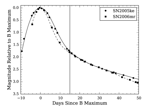
However, we have found that the very definition of $\Delta m_{15}(B)$ starts to break down as one approaches $\Delta m_{15}(B)\sim 1.7$. At this point, the change in intrinsic shape of the $B$ light-curve becomes more complicated than a simple stretch relationship and the decline in magnitude at 15 days after peak does not discriminate as well between faster and slower evolving objects. An example of this can be seen in Figure 1, where the $B$-band light-curves of SN 2005ke and SN 2006mr are over-plotted. Clearly SN 2006mr has a faster rise time and initially a faster decline after maximum, yet their rest-frame light-curves happen to intersect near day 15.

While examining the $B-V$ light-curves, however, we noticed that $\Delta m_{15}(B)$ failed to capture another trend in the photometric behavior of fast SNe Ia: the $B-V$ color as a function of time. In the next section, we examine the $B-V$ light-curves of our sample and show that the time of $B-V$ maximum may be a better parameter than $\Delta m_{15}(B)$ for the fastest evolving SNe Ia.

Figure 2.— Sample $B-V$ color-curves of 4 SNe Ia, increasing in $\Delta m_{15}(B)$ from lower-left to upper-right. The time of $B-V$ maximum for the fastest declining SN Ia, SN 2006mr ($\Delta m_{15}(B)=1.82$), is near 10 days after $B$-maximum, whereas for SN 2005M ($\Delta m_{15}(B)=0.85$), the maximum occurs approximately 40 days after $B$-maximum. A vertical dashed line is plotted at $t=30$ days to more clearly show the progression of peak times.

Figure 3.— Sample fit of the $B-V$ light-curve of SN 2005M using Equation (2). The points are the observed data, the solid line is the best-fit model, the two dashed lines are the initial and final slopes $s_{0}$ and $s_{1}$, and the two vertical lines denote $t_{0}$ and $t_{max}$.

3.2. The $B-V$ Color-Curve

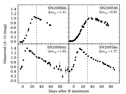
As one might expect, the shape of the $B-V$ color-curve has a more complicated morphology than either the $B$ or $V$ broad-band light-curves. The general shape of the color-curve is a local minimum (bluest) near the time of maximum, followed by a near linear increase to a local maximum (reddest) near day 30, followed by a linear decline out to later times. Lira (1996) noticed that while the early time morphology of $B-V$ varied with $\Delta m_{15}(B)$, the late-time linear decline was remarkably consistent for those objects believed to have little or no interstellar reddening. Use of this linear decline as a standard color is termed the Lira relation (see §4.1).

As one examines the behavior of the $B-V$ color-curves, it is quickly apparent that the location of the $B-V$ maximum is highly correlated with $\Delta m_{15}(B)$. Figure 2 shows 4 SNe Ia from our sample that have a range of decline rates. Clearly, the faster objects have $B-V$ maxima at earlier times compared to more slowly evolving objects.

Figure 4.— (Left) Correlation between the rest-frame time of $B-V$ maximum, $t_{max}$ with observed $\Delta m_{15}(B)$. Different plot symbols are used to indicate the spectroscopic classification of Folatelli et al. (2013) based on the system of Branch et al. (2009): squares are “Core Normal” (N), downward-pointing triangles are “Broad Line” (BL), upward-pointing triangles are “C ool” (CL), diamonds are “Shallow Silicon” (SS), and circles are unclassified. Filled symbols are further classified as “High Velocity”. There is a very good correlation for $\Delta m_{15}(B)<1.7$, whereas the two observables become decoupled for the faster decliners, which correspond to the CL type. The solid line is the fit given by Equation (3). The vertical dashed line shows $\Delta m_{15}(B)=1.1$ and the horizontal dashed line shows the corresponding value of $t_{max}=28.65$. (Right) Relationship between $s_{BV}$ and the SALT $x_{1}$ parameter. The solid line is the fit given by Equation (5).

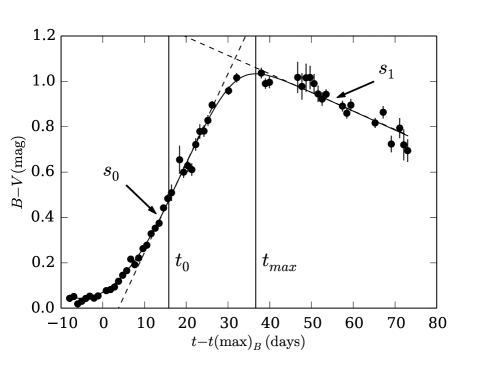
In order to investigate the $B-V$ behavior more quantitatively, we require an analytic function that will give us an estimate of the time of $B-V$ maximum as well as a fit to the late-time linear decline. We therefore require a function that is nearly linear with positive slope at early time, reaches a maximum, then transitions to linear with negative slope. The derivative of the function can therefore be described by:

$$y^{\prime}(t)=\frac{s_{0}+s_{1}}{2}+\left(\frac{s_{1}-s_{0}}{2}\right)\tanh\left(\frac{t-t_{max}}{\tau}\right),$$ (1)

where $s_{0}$ is the initial slope, $s_{1}$ is the final slope, $t_{max}$ is the location of the maximum, and $\tau$ is the length scale over which the transition occurs (the sharpness of the peak). Integrating this will give the required function. One can also add a polynomial term to capture the earliest behavior. The final function can therefore be written as:

$$y(t)= \frac{\left(s_{0}-s_{1}\right)}{2}+\frac{\tau}{2}\left(s_{1}-s_{0}\right)\ln\left[\cosh\left(\frac{t-t_{max}}{\tau}\right)\right]$$ (2)

$$+c+f_{n}(t,t_{0}),$$

where $c$ sets the overall normalization and $f_{n}(t,t_{0})$ is an order $n$ polynomial for $t<t_{0}$ and equal to 0 for $t>t_{0}$. Figure 3 shows a sample fit to the $B-V$ color-curve of SN 2005al using a quadratic to fit the early-time data. As can be seen, the two parameters of most interest ($t_{max}$ and $s_{1}$) are well-determined by the fit.

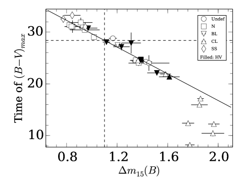
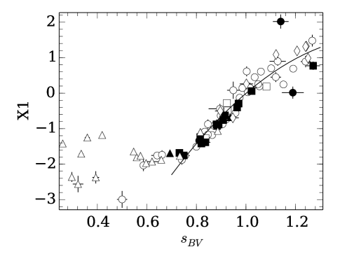
With best-fit values of $t_{max}$ from the $B-V$ color-curves, we can investigate the correlation with the light-curve shape. The left-hand graph of Figure 4 shows this correlation. Indeed, for the lower values of $\Delta m_{15}(B)$, there is a very strong correlation with the time of $B-V$ maximum. However, for $\Delta m_{15}(B)>1.7$, the correlation breaks down. We fit a straight line to the data with $\Delta m_{15}(B)<1.7$ and get the following relation between the two light-curve parameters:

$$t_{max}=28.65(13)-13.74(58)\left[\Delta m_{15}(B)-1.1\right].$$ (3)

The question now arises: is $t_{max}$ a better light-curve parameter than $\Delta m_{15}(B)$? For convenience, we now define a dimensionless stretch-like parameter $s_{BV}=\frac{t_{max}}{30\ \mathrm{days}}$. To differentiate from other parameters, we will call this the “color-stretch”. Together with Equation (3), we can convert between $s_{BV}$ and $\Delta m_{15}(B)$ using the formula:

$$s_{BV}=0.955-0.458\left(\Delta m_{15}(B)-1.1\right),$$ (4)

which is valid for $\Delta m_{15}(B)<1.7$. Likewise, we can compare $s_{BV}$ to another commonly used light-curve shape parameter: the $x_{1}$ parameter in the SALT light-curve fitter (Guy et al., 2007). The right-hand graph of Figure 4 shows the relationship between the two parameters. Clearly there is a strong correlation for $s_{BV}>0.7$. Fitting a second order polynomial, we find a formula relating $s_{BV}$ to $x_{1}$ for $s_{BV}>0.7$:

$$x_{1}=-0.006+5.98\left(s_{BV}-1\right)-5.55\left(s_{BV}-1\right)^{2}.$$ (5)

From a technical standpoint, measuring $s_{BV}$ instead of $\Delta m_{15}(B)$ offers the advantage of being relatively insensitive to reddening. To demonstrate this, we multiplied the Hsiao et al. (2007) SED by F99 reddening curves with varying amounts of extinction and constructed synthetic $B-V$ color-curves. Measuring the time of $B-V$ maximum, we found systematic shifts in $t_{max}$ of no more than 0.2 days for extinctions up to $A_{V}=3$ mag. This corresponds to changes in $s_{BV}$ of less than 1%. A disadvantage of $s_{BV}$ is that to measure it directly, one must have restframe $B$ and $V$ coverage from the time of $B$ maximum until approximately 40 days. Here again, one must resort to template fitting when such data are lacking. In the next section we examine how well $s_{BV}$ captures the photometric diversity of SNe Ia .

Figure 5.— The time of maximum in the NIR bands as a function of decline rate $\Delta m_{15}(B)$ (left) and $B-V$ color-stretch $s_{BV}$ (right). Each panel represents a separate filter in the set $iYJH$. The meaning of the plot symbols is the same as Figure 4.

3.3. NIR Light-Curves of Low Stretch SNe Ia

It has been known for some time that there is a dramatic change in the morphology of SNe Ia as one observes redward of the $r$ band (Elias et al., 1981; Ford et al., 1993; Hamuy et al., 1996b). For “normal” SNe Ia ($\Delta m_{15}(B)<1.7$), the primary maximum is followed by a secondary maximum approximately 20 days later. However, as one moves to higher $\Delta m_{15}(B)$, the secondary maximum disappears and we are left with a single peak. The question then arises: is this a continuous diminishing of the strength of the secondary peak as $\Delta m_{15}(B)$ increases (or as color-stretch decreases), or are we dealing with two separate sub-populations of SNe Ia (Krisciunas et al., 2009)? While it is not possible to answer this question definitively based on photometric data alone, finding a “missing link” between the slow decliners (with clear prominent NIR secondary peak) and the fast decliners (with no secondary NIR peak) would certainly lend credence to the former scenario. We therefore turn to examining the properties of the NIR light-curves as a function of how fast they evolve.

3.3.1 The Time of NIR Maxima

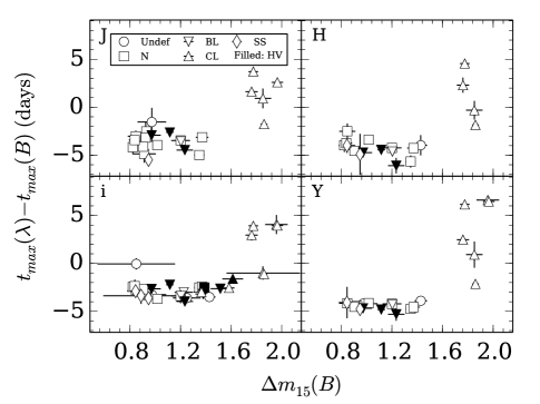
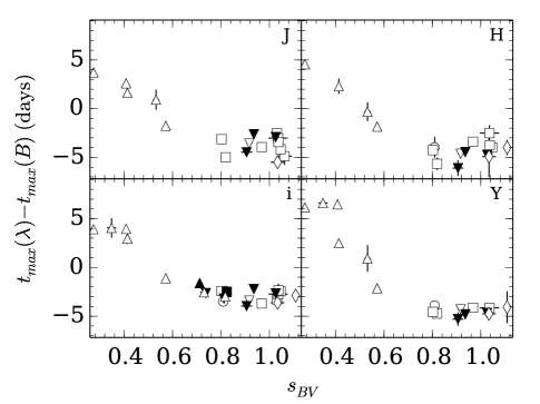
The left-hand graph of Figure 5 shows the time of first maximum of the NIR light-curves as a function of the decline rate $\Delta m_{15}(B)$. In general, slowly declining SNe Ia peak in the NIR 2-6 days earlier than $B$ band, which presents an observational challenge to obtaining NIR coverage of the peak for objects whose observations are typically triggered based on optical band discoveries. However, it has been known for some time that the faster evolving events tend to peak later (after $B$-band maximum). Examining the right-hand graph in Figure 5, it would appear that we are seeing two groups of objects: a set with early NIR peak and a set with late NIR peak, which has been seen before (Krisciunas et al., 2009; Phillips, 2012). The early NIR peak objects span the “normal” range $0.7<\Delta m_{15}(B)<1.7$, while the late NIR peak objects are exclusively in the fast-declining region $\Delta m_{15}(B)>1.7$. And in the fast-declining region, there is a large spread of peak times with no correlation with $\Delta m_{15}(B)$. On the other hand, when examining the right-hand graph of Figure 5, where we have used the $s_{BV}$ parameter, the time of NIR peak is clearly correlated with $s_{BV}$. As a result, it can be argued that the bifurcation of the fast-declining sample into early- and late-risers is an artifact of the behavior of the light-curve parameter $\Delta m_{15}(B)$.

3.3.2 The Strength of the 2nd Peak

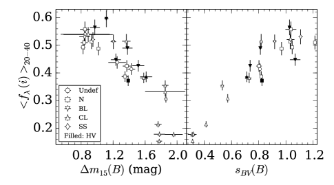
A second conspicuous feature of the NIR light-curves for normal SNe Ia is the presence of a secondary maximum. This is due to recombination of iron group elements in the supernova ejecta (Kasen, 2006) and begins to be seen in $r$ band as an inflection point, and develops into a secondary maximum in $i$ band. In the $z$ band and $Y$ band, the secondary maximum can in fact be stronger than the primary (Stritzinger et al., 2002; Burns et al., 2010). It becomes less prominent in $J$ band, and then regains strength in the $H$ band. For the fast-declining SNe Ia, however, both optical and NIR light-curves show either a very weak secondary or none at all. Following Krisciunas et al. (2001), we consider the strength of the $i$ band secondary maximum as a function of decline rate. They define $\left\langle f_{\lambda}(i)\right\rangle_{20-40}$ as the average flux (normalized to maximum) in the $i$-band from day 20 to day 40 after $B$ maximum in the rest-frame of the SN Ia. This gives a measure of the prominence of the secondary peak. In the left panel of Figure 6 we plot this as a function of $\Delta m_{15}(B)$. We see a clear correlation, albeit with significant scatter (see also Figure 8 of F10), and the fast decliners seem to separate into two groups. However, if we instead plot against $s_{BV}$ (see right panel of Figure 6), there is again a more continuous transition between the slow and fast decliners.

Figure 6.— The average normalized flux of the $i$-band between days 20 and 40 in the rest-frame of the SN as a function of the decline rate $\Delta m_{15}(B)$ (left panel) and the color-stretch $s_{BV}$ (right panel). The meaning of the plot symbols is the same as in Figure 4.

3.3.3 Continuity of Light-Curve Templates

The transition (if one exists) from the slow to fast declining SNe Ia has been a major stumbling block for light-curve fitters. Clearly, a simple stretch in time cannot account for the NIR light-curves losing the secondary peak as we go from slow decliners to fast decliners. To our knowledge, SNooPy is the only light-curve fitter that currently attempts to fit NIR light-curves for both slow and fast decliners. Up until recently, SNooPy’s NIR templates for the fast-decliners were unreliable due to two problems: 1) small numbers of fast-declining SNe Ia with well-observed light-curves, and 2) the apparent failure of the $\Delta m_{15}(B)$ parameter to distinguish between the fastest decliners.

Figure 7.— Light-curves of 11 SNe Ia for which $1.5<\Delta m_{15}(B)<2.0$, binned into 5 intervals. The left panels show $B$ band and right panels show $Y$ band. The individual SNe Ia are labeled with different symbols. The average SNooPy light-curve template for the bin is shown as a black line. Note that one panel is missing data due to the fact that the object SN 2004gs has no NIR observations.

Figure 8.— Same as Figure 7, but using the color-stretch parameter, $s_{BV}$, to bin the SNe Ia having $0.2<s_{BV}<0.7$. Note that one panel is missing data due to the fact that object SN 2008R has no NIR observations.

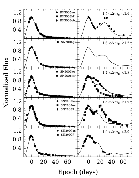
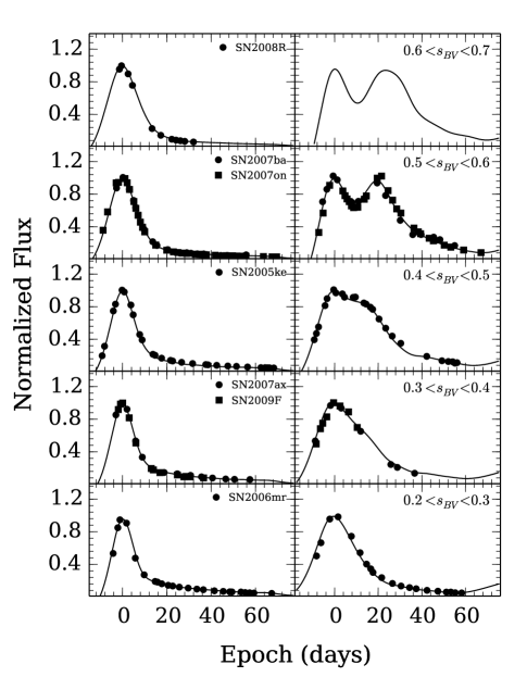
Figure 7 shows the sorting of the 11 fastest decliners in the SNooPy training sample into bins of $\Delta m_{15}(B)$. One can clearly see the problem: while the $B$-band light-curves seem to be sorted out correctly (with the possible exception of SN 2006mr), the $Y$-band light-curves clearly do not follow any kind of continuous progression from $\Delta m_{15}(B)\simeq 1.5$ to $\Delta m_{15}(B)\simeq 2.0$. The same holds true for the other NIR bands. The situation, however, is completely different when one uses the $s_{BV}$ parameter instead. In Figure 8, we can see that SN 2006mr, which is clearly the fastest declining of the SNe Ia, is now the lowest color-stretch. SN 2007ba and SN 2007on are now categorized as slower events. This has the very noticeable effect that the $Y$-band light-curves now show a more continuous progression from $s_{BV}\simeq 0.2$ to $s_{BV}\simeq 0.6$. Another notable feature is that SN 2005ke now looks very much like a transition object, having no secondary peak, but clearly an inflection point.

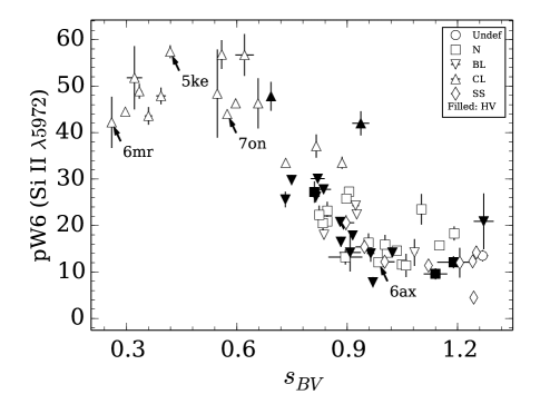
To further investigate this, we examined the spectra of 4 representative objects in this range of $s_{BV}$: SN 2006ax ($s_{BV}=0.985$), SN 2007on ($s_{BV}=0.574$), SN 2005ke ($s_{BV}=0.419$), and SN 2006mr ($s_{BV}=0.260$). Figure 9 shows the spectra of these 4 objects near maximum light. SN 2005ke shows several spectroscopic features common to the “Cool” SNe Ia: prominent Ti II and Si II $\lambda 5972$. On the other hand, it shows an intermediate strength in the S II “W” feature. The presence of Ti II is highly sensitive to effective temperature and will therefore turn on rather abruptly, making any transition with $s_{BV}$ equally abrupt. Another feature know to be correlated with light-curve width is Si II $\lambda 5972$ (Folatelli et al., 2013). In Figure 10 we plot the pseudo-equivalent width of Si II $\lambda 5972$ from Folatelli et al. (2013) as a function of $s_{BV}$. Interestingly, there is a more complicated relation than the linear trend seen with $\Delta m_{15}$. In particular, there seems to be very little trend for $s_{BV}<0.5$.

While it remains unclear whether $s_{BV}$ is in fact a “better” parameter than $\Delta m_{15}$ in predicting the physics of the SNe Ia, the fact remains that it does produce a much more continuous family of light-curve templates for the faster-declining objects. For this reason, the SN Ia template-fitting package SNooPy will incorporate templates parametrized by $s_{BV}$ and we will adopt it as our shape parameter for the remainder of the paper. It is also unclear whether $s_{BV}$ will present a superior alternative when analysing high-redshift SNe Ia for the purposes of cosmology, as the fast-declining events are less numerous and significantly fainter than normal SNe Ia.

4. Intrinsic Colors of SNe Ia

As shown by numerous groups (e.g., Tripp, 1998; Phillips et al., 1999; Astier et al., 2006; Folatelli et al., 2010, hereafter F10), in order to correct for the interstellar reddening and any other intrinsic color-luminosity relationship for the purposes of determining distances, it suffices to use the observed colors. However, if we wish to understand what is causing the observed color distribution of SNe Ia or wish to measure their intrinsic luminosities, then we must determine the intrinsic colors of these objects in order to separate out the contribution from dust extinction along the line of sight. In the following sections, we present two methods for determining these intrinsic colors: the Lira relation and statistical inference from the observed pseudo-colors.

Figure 9.— Comparison of the spectra of 4 SNe Ia near maximum light. The spectra are labeled with the object’s name, phase, and color-stretch $s_{BV}$. Several prominent spectral features are also labeled: Ti II $\lambda 4250$, the S II “W” feature $\lambda\lambda 5454,5640$, Si II $\lambda 5972$, Si II $\lambda 6355$, O I $\lambda\lambda 7772,7775$, and the Ca II IR triplet $\lambda 8579$. Note that due to high expansion velocities, these lines will appear to the blueshifted relative to their rest wavelengths in observed spectra.

Figure 10.— The pseudo-equivalent width of the Si II $\lambda 5972$ feature as a function of the color-stretch $s_{BV}$. The four objects from Figure 9 are labeled. The meaning of the plot symbols is the same as in Figure 4.

4.1. The Lira Relation Revisited

Lira (1996) discovered that the $B-V$ color-curves of SNe Ia, while showing significant variation at early times, all seem to converge to a linear decline at late times. By fitting a line to the late-time $B-V$ data, one could then determine the amount of reddening relative to an ensemble of objects for which it is assumed (see §4.2) there is little to no reddening (Phillips et al., 1999). As far as could be seen with the data at the time, there did not appear to be any significant difference in the late-time colors of either slow or fast decliners, providing a truly standard color. With our improved number of objects and homogeneous photometry, we re-visit the Lira relation, as was done in F10.

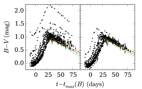
Figure 11 shows the $B-V$ light-curves of 40 of our SNe Ia, for which reliable times of $B$-maximum are measured and sufficient late-time ($t-t_{max}>30$ days) $B$ and $V$ photometry are observed to fit the Lira relation. In the left-hand panel, we plot the rest-frame $B-V$ color-curves corrected for MW reddening derived from Schlafly & Finkbeiner (2011). In the right-hand panel, we offset each light-curve downward such that the resulting late-time data show a minimum dispersion with respect to the Lira relation from F10, which amounts to 0.04 mag rms. In both panels we plot the Lira relation derived by F10 in red. It is apparent that there is a systematic difference between the mean slope of the corrected data and the F10 fit, which was done using a subset of the sample of SNe Ia that were believed to have suffered little or no reddening. In order to determine the reason for the difference in slope, we examine each object individually.

Figure 11.— The $B-V$ color-curves for 40 SNe Ia in our sample. The left panel shows $B-V$ corrected for Milky-Way extinction only, whereas the right panel shows $B-V$ curves shifted downward so as to minimize the residuals with respect to the Lira relation from F10, shown as a solid red line in both panels. The new fit given by Equation (6) for $s_{BV}=1$ is plotted as a solid green line and the observed range of slopes are plotted as dashed green lines.

Figure 12.— The slope of the late-time $B-V$ color-curve as a function of the color-stretch, $s_{BV}$ (left panel), and the $B-V$ color at day 45, $(B-V)(45)$ (right panel). The meaning of the symbols is the same as in Figure 4, however objects whose $B-V$ at day 45 is greater than 1.0 mag are labeled in red and two additional objects (SN 1991T and SN 1998bu) are labeled with stars. The solid line in the left-hand panel is a fit to the data excluding the red points. The horizontal dashed line and dark grey shaded region shows the slope from F10 and the horizontal solid line and lighter shaded region show the median and standard deviation of the slopes from this paper.

For this purpose, we employ Equation (2) to examine the slopes ($s_{1}$) of the late-time linear portion of the $B-V$ light-curves for our sample. Aside from getting an improved estimate of a global Lira relation, we can examine in detail whether there are any trends with respect to light-curve shape, reddening, and any other properties we desire.

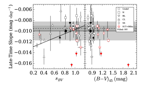
Figure 12 shows the late-time slope of the $B-V$ color-curves as a function of $s_{BV}$ (left panel) and $B-V$ color at day 45 (right panel). There appears to be a trend such that the fastest evolving objects tend to have late-time $B-V$ slopes that are steeper (more negative) than “normal” objects. This is to be expected if low-color-stretch objects simply evolve more quickly than high-color-stretch objects. We note, however, that the trend is not nearly as strong as the $1/s_{BV}$ trend one would expect. We also see that there are significant outliers with $s_{BV}\simeq 1$ and very steep slopes. These also correspond to objects with larger than average colors and we have labeled points for which $(B-V)(45)>1$ in red. Objects that have redder colors tend to have steeper late-time slopes. Looking at the most extreme case, SN 2006X, it is likely that the steepness of the late-time slope is due a light-echo caused by scattering of light by dust into our line of sight (Wang et al., 2008). It is therefore possible that the more moderately reddened cases also have scattering of light into the line-of-sight, only to a lesser degree. Two other objects are known to have light-echoes: SN 1991T (Schmidt et al., 1994) and SN 1998bu (Cappellaro et al., 2001). We plot them in Figure 12 as star symbols. SN 1998bu has a late-time slope consistent with most in our sample, whereas SN 1991T follows the trend of the redder objects. While the light-echo in SN 2006X is observed one month after maximum, those in SN 1991T and SN 1998bu are detected much later (600 and 500 days after $B$ maximum, respectively). It is possible that SN 1991T, like SN 2006X, had a light-echo at earlier times that was missed due to the pecularity of this object. Then again, being a peculiar SN Ia, the steeper late-time $B-V$ slope could be due to the physics of the object. It has been argued that this change in slope could be due to CSM around these objects (Förster et al., 2013), which is supported by the fact that both SN 2006X and SN 2007le are known to have CSM and show very low $s_{1}$.

As it is not entirely clear whether or not the trend of slope with color is intrinsic to the SN Ia, we discard the red objects and fit a linear relation between the late-time slope and $s_{BV}$, obtaining $ds_{1}/ds_{BV}=0.004\pm 0.001$, which is shown in the left panel of Figure 12 as a solid line. We also solve for an intrinsic $(B-V)(45)$ color and scatter by modeling the observed distribution as the convolution of a Gaussian with an exponential distribution with scale length $\tau_{BV}$ (see Jha et al., 2007). We obtain $(B-V)(45)=0.78\pm 0.04$ and $\tau_{BV}=0.19\pm 0.03$. Together, these results give us an updated Lira relation:

$$(B-V)(t) = 0.78(04)-\left[0.0097(5)-\right.$$ (6)

$$\left.0.004(1)\left(s_{BV}-1\right)\right]\left(t-t_{max}-45\right).$$

Indeed, the slope one obtains for a $s_{BV}=1$ object is quite consistent with the slope derived in F10, shown as a dashed horizontal line and dark shaded region in Figure 12. The green solid line in Figure 6 represents Equation (6) for $s_{BV}=1$ whereas the dashed green lines are for $s_{BV}=0.2$ and $s_{BV}=1.2$.

4.2. Low-Reddening Sample vs. Blue Edge

In order to derive the Lira relation, Lira (1996) used a “low reddening” sample of SNe Ia to anchor the colors to a standard intrinsic locus. These objects were thought to have very little dust due to their distance from the host and/or the host being an early type galaxy, which are thought to have very little interstellar gas and dust (Sternberg et al., 2011). Later work by Phillips et al. (1999) and F10 used similar arguments to construct a set of objects whose colors were believed to be intrinsic, though also adding the requirement that Na I D absorption be absent from the objects’ spectra. While this is a simple way to throw out reddened objects for the purpose of determining intrinsic colors, it also eliminates objects that have a small projected impact parameter in a late type host which, if in the foreground, could have no interstellar reddening. These objects also provide information and we would like to keep them in the “low reddening sample”.

Furthermore, using host type and proximity as arguments for inclusion in the reddening-free sample is predicated on the assumption that the extinction is caused by the interstellar medium of the host, whereas some portion of the extinction could be caused by dust associated with the SN Ia progenitor system itself. For this reason, we would like to refrain from relying on the identification of a reddening-free sample.

To this end, instead of categorizing the objects, we can exploit the fact that extinction can only make objects redder. We therefore expect that the bluest objects will define the intrinsic colors and therefore we seek a “blue edge” to the data. From a Bayesian perspective, we could simply apply a prior that the $B-V$ color excess, $E(B-V)$, be strictly positive. However this does not suffice, as this does not preclude arbitrarily large positive values of $E(B-V)$ and arbitrarily large negative intrinsic colors. We therefore must also insist that the likelihood that an object is reddened decrease for large values of $E(B-V)$. The prior will therefore be peaked and we address the functional form of the prior in the next section.

4.3. Inferring Intrinsic Colors

Under the assumption that the extinction suffered by the SN follows a well-defined dust law that is not uniquely grey, the amount of reddening in each filter pair will be different. The most commonly used parameterization has two quantities: $E(B-V)$ and the ratio of total-to-selective absorption in the $V$ band, $R_{V}$. The color excess sets the optical depth, while $R_{V}$ is related to the distribution of dust grain sizes (Weingartner & Draine, 2001). We further assume that the intrinsic color of each SN Ia is a smooth function of color-stretch $s_{BV}$ and model this relationship as an $N$th order polynomial in $P_{j}^{N}$. The observed colors are then given by

$$\left(B-m_{j}\right) = P_{j}^{N}\left(s_{BV}-1\right)+\Delta A_{j}\left(E(B-V)_{host},R_{V}\right)+$$ (7)

$$\Delta A_{j}\left(E(B-V)_{MW},3.1\right),$$

where $m_{j}$ is the observed rest-frame magnitude in filter $j=\left\{u,g,r,i,V,Y,J,H\right\}$, $\Delta A_{j}=A_{B}-A_{j}$ is the differential extinction between $B$-band and filter $j$, being a function of the host galaxy color excess $E(B-V)_{host}$, the host galaxy reddening parameter $R_{V}$, and the MW foreground color excess $E(B-V)_{MW}$. $\Delta A_{j}$ is determined numerically by multiplying the Hsiao et al. (2007) SED with the appropriate reddening curve and computing synthetic photometry using the CSP filter functions. We assume the canonical MW value $R_{V}=3.1$. The form of the function $\Delta A_{j}\left(\right)$ is dictated by the choice of reddening law. For this paper, we consider the reddening laws of Cardelli et al. (1989); O’Donnell (1994) (hereafter CCM+O), F99, and the CSM-motivated reddening law of Goobar (2008, hereafter G08). For each color, we also solve for an intrinsic scatter $\sigma_{xy}$. Chotard et al. (2011) and Scolnic et al. (2014) have shown the importance of accounting for intrinsic color variations and it is our intent to do so with these parameters.

It is important to realize that the CCM+O and F99 dust laws are empirical fits to observations of stars in our own MW’s interstellar medium (ISM). These fits were made to observations of stars whose lines of sight have values of $R_{V}$ that cover the range $2.6\leq R_{V}\leq 5.6$ (Cardelli et al., 1989; Fitzpatrick, 1999). Therefore, allowing $R_{V}$ to vary beyond these limits constitutes an extrapolation of these fits, which of course is always dangerous. As we will see, several of our fits favor $R_{V}<2$, where the dust laws are not valid. Nevertheless, the parameterization of CCM+O, being of the form $a+b/R_{V}$, is very smooth and does remarkably well at reproducing the observed colors of the reddest SNe Ia. We therefore allow $R_{V}$ to vary below $R_{V}=2.6$, but refrain from inferring anything about the physics of the dust or ISM.

For $N_{F}$ filters, we have $N_{F}-1$ independent colors. For each color, we will fit the coefficients of $P_{j}^{N}$. For each supernova, we will compute a separate reddening $E(B-V)_{host}$. The remaining parameter of interest, $R_{V}$ can either be solved as a universal value for the whole sample of SNe Ia, or we can try to fit a separate $R_{V}$ for each object. We do both in the next sections. We also investigate whether the polynomial $P_{j}^{N}$ should be a linear fit ($N=1,$ as was done in F10), or if the data warrant a quadratic ($N=2$).

Due to the multiplicative nature of $R_{\lambda}$ and $E(B-V)_{host}$ in the $\Delta A_{j}$ term of Equation (7), these parameters will be highly covariant. Also, as the $E(B-V)_{host}$ becomes small, the model becomes less sensitive to $R_{V}$. We therefore require priors on these values. For $E(B-V)_{host}$, we investigate three priors: 1) assigning zero reddening to the “low reddening sample” (LRS) and uniform priors for every other object; 2) an exponential prior for all objects as used by Jha et al. (2007); and 3) a truncated Cauchy distribution, which has a longer tail to large values. For $R_{V}$, we investigate four priors: 1) a universal $R_{V}$ for the entire sample with uniform prior; 2) separate $R_{V}$ for each SN Ia with uniform priors; 3) separate $R_{V}$ drawn from an N-component Gaussian mixture model; and 4) separate $R_{V}$ drawn from one of $N$ independent Gaussians binned by $E(B-V)_{host}$. The last of these is motivated by the results of Mandel et al. (2011) who show a linear trend between $R_{V}$ and $A_{V}^{-1}$. These priors are discussed in more detail in Appendix A.

Figure 13.— Observed rest-frame colors, corrected for foreground MW extinction, are plotted versus color-stretch. The meaning of the symbols is the same as in Figure 4. Several best-fit models for the intrinsic color loci are plotted as lines. Solid lines are fits to the slow sample only, while dashed lines are fits to the entire sample. Black lines are fits using the Cauchy prior, while blue lines are fits using the LRS prior.

Figure 14.— Same as Figure 13, but with both foreground MW and host galaxy extinction removed. The extinctions derived from the model with the Cauchy prior were used and the best-fit intrinsic color loci are plotted as a dashed blue line.

4.4. Results

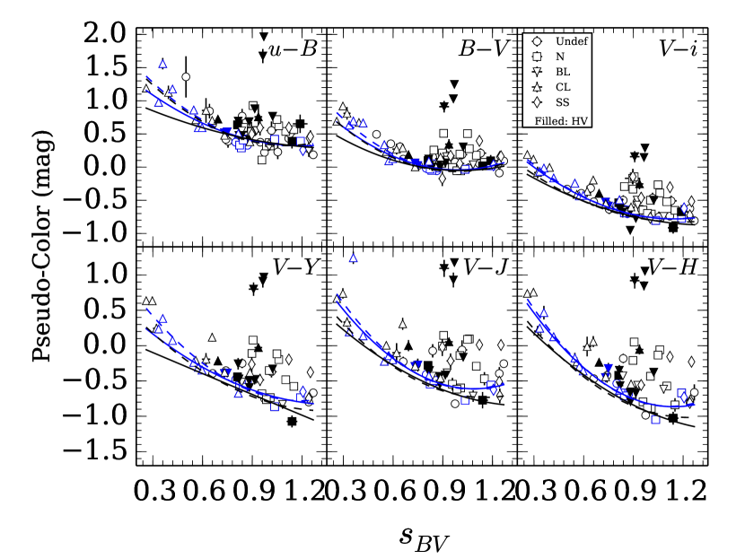
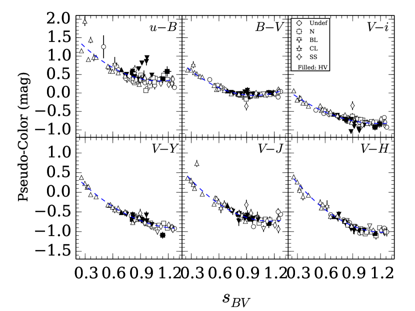
In general, the Bayesian method we have developed does a good job of finding the locus of bluest colors in our sample. Figures 13 and 14 show the observed and host galaxy extinction-corrected pseudo-colors, respectively. Aside from investigating the effects of using different priors on our model, we also investigated the effects of including different subsamples of our data by filtering on two observables: the color-stretch and $B-V$ pseudo-color. We produced 2 subsamples: 1) the “slow” sample consisting of all objects with $s_{BV}>0.5$, which primarily excludes the SN 1991bg-like objects, and 2) the “blue” sample that excludes objects with $\left(B_{max}-V_{max}\right)>0.5$, eliminating the most heavily reddened objects. We now proceed to describe the results of fitting with different priors and samples.

4.4.1 Order of the Color-Stretch Relation

The first thing we determined was whether or not the intrinsic color-stretch relations, $P_{j}^{N}(s_{BV})$, require a linear or quadratic relation. To accomplish this, we introduce a selection function $S(p_{1},p_{2})$ into our likelihood which selects a linear color relation, ($N=1$) with probability $p_{1}$ and the quadratic color relation ($N=2$), with probability $p_{2}$. In this way, the MCMC chains will spend some time trying the linear model and some time trying the quadratic. We can compute the posterior probability $P(N)$ by counting nodes in the chain. From that we can compute the odds ratio:

$$O=\frac{P(N=2)}{P(N=1)}\frac{p_{1}}{p_{2}}.$$ (8)

The odds ratio gives a measure of the likelihood of one model versus the other, giving us the ability to select one if the data so warrant. Note that the probabilities $P$ in Equation (8) are computed by marginalizing over all parameters and so there is a built-in “Occam factor” that penalizes the $N=2$ model as it has one more free parameter (Gregory, 2011). Several pilot runs of our MCMC gave odds factors between 16 and 88 in favor of the quadratic model. The lower values of the odds ratio occur when we do not use the LRS prior and restrict the data to $s_{BV}>0.5$. This can easily be seen in Figure 13 where fits to the data without the “low reddening” prior tend to have less curvature than when the “low reddening” sample are constrained to have zero reddening. In either case, an odds ratio of greater than 10 is considered reasonably strong evidence (Jeffreys, 1961) to favor the quadratic model over the linear one and we continue throughout with quadratic solutions for the SN Ia intrinsic colors.

Figure 15.— Comparison of derived color excesses $E(B-V)_{host}$. In the left panel, we plot the difference between $E(B-V)_{host}$ inferred using the exponential and Cauchy priors versus the color-stretch $s_{BV}$. In the right panel, we compare the Cauchy and LRS priors. The error bars are the 68% confidence intervals determined from the posterior distributions for each quantity.

4.4.2 The $E(B-V)_{host}$ Prior

When solving for the intrinsic colors, the factor that has the largest effect is whether or not we use the LRS prior. In most cases, $P_{j}^{N}$ ends up having a higher curvature when we use the low reddening sample. This is most notable in the optical minus NIR colors $V-Y$, $V-J$, and $V-H$, where there are a significant number of objects at high color-stretch that are bluer than the low reddening sample and therefore tend to straighten out the intrinsic color-curves. This is easily understood as the LRS prior, being associated with specific objects, implicitly defines a color-stretch dependence on the intrinsic colors, whereas the Cauchy and exponential priors apply to the sample as a whole and are “color-stretch blind”. At the high- and low-color-stretch ends of the distribution, there are relatively few objects and so the solution for the Cauchy and exponential prior has more freedom at those ends.

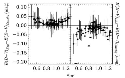
The resulting $E(B-V)_{host}$ color excesses also differ the most when comparing the LRS prior to the analytic priors. The left panel of Figure 15 shows the difference between the color excesses from the exponential and Cauchy priors. There is a systematic offset of about 0.02 mag in the sense that the exponential prior produces higher extinctions and there is a systematic difference with $s_{BV}$, though both effects are less than the 1-$\sigma$ errors in the extinctions themselves. The right panel of Figure 15 shows the difference between the color excesses from the Cauchy and LRS priors. One can see there is a much larger offset in the sense that the LRS prior produces lower color excesses and there is a more pronounced systematic with respect to $s_{BV}$. This is also easily understood as Figure 13 shows that the intrinsic colors from the LRS are significantly redder than those from the Cauchy or exponential priors. In both cases, the systematic trend in the differences with $s_{BV}$ is due to low- and high-$s_{BV}$ ends having fewer objects so that the choice of prior has more of an effect.

Along with varying the priors, we also varied the sample used to fit the intrinsic colors. In particular, we were interested in whether the fast-declining objects could be fit together with the normal Ia’s. Figure 13 shows the best-fit intrinsic colors obtained when excluding (solid line) and including (dashed line) the fast-declining SNe Ia. The fits are remarkably close. Indeed, when using the color-stretch parameter $s_{BV}$ instead of $\Delta m_{15}$, the fast-declining objects seem to lie on a smooth extension to the color loci of the normal objects.

For reasons stated above, we prefer to be agnostic about the reddening and go forward with the results obtained without using the LRS. We also adopt the Cauchy prior for the reddening as it allows a higher probability for larger reddenings. Table 2 lists the fits to the intrinsic color coefficients when using different subsamples and assuming different priors. It also tabuates the intrinsic scatter in the colors. These vary between 0.05 and 0.15 mag. The optical colors $B-V$ and $g-r$ have the lowest intrinsic widths, followed by the optical-NIR colors. The $u-B$ color stands out as having a partcularly large scatter. We consider the results for the reddening law in the next sections.

4.4.3 Fitting a Single Reddening Law

If we use a simple uniform prior for $R_{V}$ that is universal for the entire sample of SNe Ia, we find that the recovered value depends on the subsample of objects we fit and the form of the reddening law. Table 3 lists the resulting values of $R_{V}$ for these different cases. The sensitivity to subsample was seen in our earlier work (F10) and continues with our larger sample of objects. Generally speaking, when we include those SNe Ia with pseudo-colors redder than $B_{max}-V_{max}\simeq 0.5$, the resulting value for $R_{V}$ tends to be lower.

In all cases, the F99 reddening law results in higher $R_{V}$ than CCM+O. This is simply due to the different behaviors of either reddening law as we extrapolate to $R_{V}<2.6$. All we can say is that when the reddest SNe Ia are removed from the analysis, the resulting value of $R_{V}=2.15\pm 0.16$ for the F99 reddening law is well below the typical value for the MW. For the remainder, we will primarily use F99 to describe ISM dust, however we also include results using CCM+O in our tables for comparison and in order to be consistent with previous publications.

The dependence of $R_{V}$ on subsample was seen in F10 and it was argued that a possible explanation was that the reddest SNe Ia could have increased extinction due to the proximity of dust local to the progenitor system (G08). Indeed, a detailed analysis in F10 of the extinction as a function of wavelength seemed to favor the G08 power-law over the standard CCM+O law due to its ability to better fit the $u$-band extinction. We therefore also attempt to fit the G08 reddening law:

$$\frac{A_{j}}{A_{V}}=1-a+a\left(\frac{\lambda_{j}}{\lambda_{V}}\right)^{-p},$$ (9)

where $\lambda_{j}$ is the effective wavelength of filter $j$. The differential extinction is therefore

$$\Delta A_{j}=A_{V}a\left(\left(\frac{\lambda_{B}}{\lambda_{V}}\right)^{-p}-\left(\frac{\lambda_{j}}{\lambda_{V}}\right)^{-p}\right),$$ (10)

where we see that $A_{V}$ and $a$ are completely degenerate. We can therefore only make inferences on the product of these two parameters. Column 4 of Table 3 lists the best-fit values for the power index $p$.

Figure 16.— The residuals in $u-B$ for the three different reddening laws used in this paper. The gray shaded regions denote the intrinsic dispersion in the $u-B$ color. The symbols have the same meaning as Figure 4. Four objects with particularly high residuals are labeled.

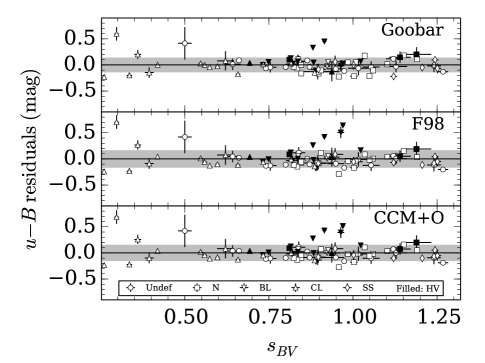
As with fitting for $R_{V}$, the resulting values of $p$ depend quite a bit on the data. We fit with the same 4 scenarios as before. As with CCM+O and F99, removing the reddest objects results in a less steep reddening law, and there is a slight dependence on inclusion of the $u$ band.

Figure 17.— The residuals in $u-B$ for the F99 reddening law versus the pseudo-equivalent width of Ca II H & K lines from Folatelli et al. (2013). The BL HV objects with the highest $pW1$ are labeled. The symbols have the same meaning as Figure 4. Several BL-HV objects are labeled.

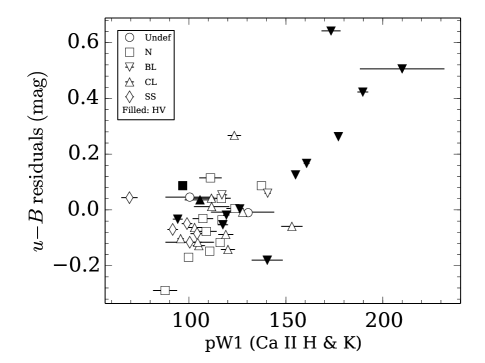
While it remains true that the $u$-band color excess for the two reddest objects (SN 2005A and SN 2006X) are better fit by the G08 power-law, these seem to be the only two and it may simply be a statistical fluke. Figure 16 shows the residuals in the color model for $u-B$. Clearly, SN 2005A and SN 2006X show a better fit, but very few others show a similar improvement. SN 2006X is known to have CSM (Wang et al., 2008), which was the motivation for the G08 power-law, so it is interesting that it fits better. However, SN 2007le is also known to have CSM (Simon et al., 2009), and yet it is fit equally well by CCM+O and F99. It is also conspicuous that the largest outliers are all spectroscopically classified as broad line (BL) and high-velocity (HV). This could indicate that it is spectral features that are responsible for the non-standard $u-B$ colors. To investigate this, we plot the $u-B$ residuals as a function of the pseudo-equivalent width of the Ca II H & K lines, $pW1$ from Folatelli et al. (2013). This is shown in Figure 17. Clearly, the objects with high $pW1$ have the highest residuals. We therefore conclude that the anomalous $u-B$ colors of these BL objects are due to their prominent Ca II lines rather than an anomalous reddening law due to CSM.

As a check, we can easily estimate the change in $u-B$ color due to a change in $pW1$. We start by measuring synthetic $u$ and $B$ flux from the Hsiao et al. (2007) SED. We then artificially remove the Ca II H & K lines by interpolating the continuum. The flux is then re-measured and a flux decrement in each filter is computed. This flux decrement is scaled from the Hsiao et al. (2007) $pW1=108$Å to $pW1=200$Å and removed from the original $u$ and $B$ fluxes. The resulting change in $u$ is 0.33 mag fainter, while the change in $B$ is 0.03 mag fainter, so that the change in $u-B$ is 0.3 mag redder, consistent with the effect seen.

In a recent paper, Mandel et al. (2014) presented evidence that BL-HV events show intrinsic color differences in $B-V$ and $B-R$ of $\sim 0.05-0.10$ mag with respect to normal SNe Ia, and that these differences originate in the $B$ band. The intrinsic colors for the CSP sample plotted in Figure 13 show similar deviations in $B-V$ for the same BL-HV events in our sample that display anomalous u-B colors. Foley & Kasen (2011) have argued that this is a natural expectation for HV objects since for saturated lines, as ejecta velocity increases, the width of the line will also increase. This, in turn, leads to larger equivalent widths and generally higher opacity in wavelength regions where there are many strong lines. This effect is particularly strong in $u$ due to the strength of the Ca II H & K absorption.

This trend with Ca II can also be seen in the work by Chotard et al. (2011), who modeled a reddening law based on spectrosopic obserations of SNe Ia. After correcting for decline rate, the reddening law had sharp features due to variaions in the strength of Ca II H & K, Ca II NIR triplet, and Si II $\lambda 6355$. They apply a color correction based on the Ca II H & K strength, which is precisely what we see in Figure 17.

Figure 18.— Montage of several color excess vs. color excess plots. Each SN Ia is a single point in these diagrams. The meaning of the symbols is the same as in Figure 4. The $V$-NIR color extinctions are labeled on the y-axes. Two representative reddening laws are plotted in each panel: $R_{V}=3.1$ is plotted as a dashed line, while $R_{V}=1.7$ is plotted as a solid line. Objects with peculiar color excesses are labeled.

4.4.4 Fitting Individual $R_{V}$

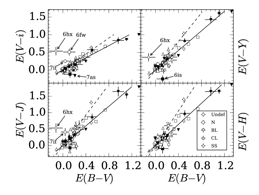
Given that the derived value of $R_{V}$ depends on the sample used, it is natural to ask whether certain objects are driving the solution, particularly those with larger color excesses which have a greater “pull”. In Figure 18 we show a montage of the extinctions in different NIR filters relative to $E(B-V)_{host}$. In these extinction-extinction plots, a fixed reddening law, $R_{V}$, should produce a correlation with fixed slope equal to $(R_{X}-R_{Y})$ where $X$ and $Y$ correspond to the particular filter combination and the $R_{\lambda}$ values are dependent on the value of $R_{V}$ through the reddening law. Clearly, there is a large spread in the correlation with a tendency to small values of $R_{V.}$ Because of this, we allow the reddening coefficient $R_{V}$ to vary for each SN Ia in the sample.

As a first step, we again use uniform priors on the individual $R_{V}$. For objects with very little extinction or no NIR photometry, $R_{V}$ will be very poorly constrained. Nevertheless, the inferred $E(B-V)_{host}$ and intrinsic color loci will be well-defined. We are primarily interested in those objects for which $R_{V}$ can be constrained and require only uniform priors.

Figure 19.— The best-fit $R_{V}$ as a function of the best-fit color excess $E(B-V)_{host}$ for each individual SN Ia using the Cauchy prior. Only objects for which $R_{V}$ was significantly constrained are plotted. The error-bars are drawn to show the correlation between the two variables and correspond to the principal axes of the 1-$\sigma$ error ellipse for each point. The meaning of the symbols is the same as Figure 4. The two horizontal lines show the typical value $R_{V}=1.7$ derived for SNe Ia and the canonical value $R_{V}=3.1$ for the Milky-Way. The mean and standard deviations of the binned prior from §4.4.6 are plotted as red points and error-bars.

Figure 20.— The color excesses $E(B-\lambda)$ normalized by $E(B-V)_{host}$ as a function of inverse wavelength for a sample of 8 SNe Ia with a range of reddening laws. In the left panel, the solid lines are CCM+O laws with different values of $R_{V}$ as labeled to the left of each curve. In the right panel, G08 power-law fits are plotted instead. The value of $p$ is labeled to the left of each line.

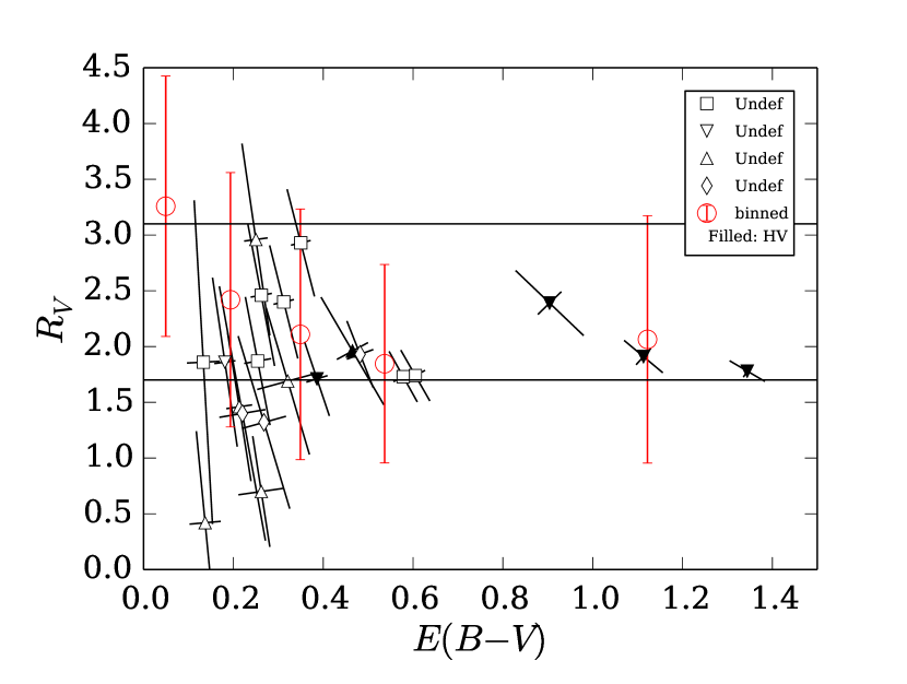
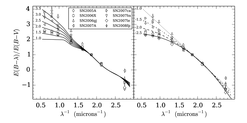
The results of fitting $E(B-V)_{host}$ and $R_{V}$ are shown in Figure 19 and tabulated in columns 6, 7, and 10 of Table 1. As expected, the value of $R_{V}$ becomes unconstrained as the amount of reddening tends to zero. In general, it would seem that the objects with moderate color excesses ($0.2<E(B-V)_{host}<0.5$) have a range of $R_{V}$ from the rather low values that have been endemic of SN Ia studies to values more in line with the canonical Milky-Way value of $R_{V}=3.1$, though these seem to be in the minority. All the more reddened objects tend to the low value of $R_{V}\sim 1.7$. Figure 20 shows a plot similar to Figure 14 in F10 where we plot the color excess in different filters as a function of inverse wavelength. We have normalized the color excesses by $E(B-V)_{host}$ in order to focus on the shape of the extinction curve. CCM+O curves with a range of values of $R_{V}$ are shown for reference. Clearly, the colors of some objects like SN 2006gj are consistent with values closer to the Milky-Way value of $R_{V}=3.1$ whereas colors of objects like SN 2007le would imply a lower value of $R_{V}\sim 1.7$. Others have attempted to model a relationship between $R_{V}$ and the observed colors (Mandel et al., 2011), however in the absence of any theoretical model to motivate such a relationship, and significantly fewer objects in our sample, we will not do so at this time. It is fair to say, however, that a simple one-parameter description of the extinction suffered by SNe Ia is insufficient to explain the diversity of inferred values of $R_{V}$.

There are 4 objects which prefer very low values of $R_{V}$, such that they give us upper limits. These objects, SN 2004eo, SN 2005ke, SN 2007ba, and SN 2008gp, have moderately red optical colors, but very blue optical-NIR colors. These cannot be explained with any reasonable reddening law and must be due to intrinsically peculiar colors or systematic errors in the NIR photometry. We have already argued that SN 2005ke is a transitional object between fast and normal SNe Ia and SN 2007ba has a similar $s_{BV}$. They, and SN 2004eo, are classified as spectroscopic type CL, while SN 2008gp is unclassified. However, there are other CL types that have ranges of $R_{V}$ that are perfectly normal. Unfortunately, we do not possess NIR spectra of these objects and cannot determine whether there are spectroscopic peculiarities in the NIR.

4.4.5 Inferring Milky-Way Extinctions

Throughout this paper, we have assumed foreground MW color excesses from Schlafly & Finkbeiner (2011). While we include the error for these measurements in our analysis, one might be concerned that there may be a systematic difference between the true color excess and the Schlafly & Finkbeiner (2011) values. In order to test this, we can look at objects whose host galaxy extinctions are expected to be low (due to host type, projected distance, and lack of Na I absorption), yet have significant MW extinction according to Schlafly & Finkbeiner (2011).

There are three such objects in our sample: SN 2006kf ($E(B-V)_{MW}=0.210$), SN 2008bc ($E(B-V)_{MW}=0.225$), and SN 2008ia ($E(B-V)_{MW}=0.195$). In a trial run, these objects’ foreground extinctions were artificially set to zero, allowing us to determine the foreground extinction based on the observed colors of the SNe rather than extinction maps. The results are given in Table 4. The values of $E(B-V)_{host}$ are quite close and show no sign of significant systematic difference, though it is difficult to be certain with only three objects. The derived values of $R_{V}$ are consistent with the spread in values associated with MW sight-lines (Cardelli et al., 1989; Fitzpatrick, 1999).

4.4.6 General $R_{V}$ Priors

We finish with an attempt to construct a prior for $R_{V}$ that can be used when either 1) the extinction is too low or 2) there is insufficient filter coverage. We do this in two ways: by constructing a Gaussian mixture model as done in Kelly (2007) for all objects and splitting the objects into bins of $E(B-V)_{host}$ and constructing an independent Gaussian distribution for each bin.

The Gaussian mixture model is simply a sum of $N$ Gaussians, forming a composite prior that can have larger wings or multiple peaks. Details of the construction of this prior can be found in the Appendix and Kelly (2007). We run our MCMC analysis using the same sub-samples and filter sets as in §4.4.3. We find that two Gaussian components are sufficient, though the second is barely significant. Table 5 summarizes the values of the mixture model’s hyper-parameters. It is evident that the parameters are quite insensitive to which subsample and filter set we use. We can therefore use any to represent a prior on $R_{V}$ for future studies.

Our second approach is to bin the data by $E(B-V)_{host}$ and solve for an independent single Gaussian prior for each bin. The hope is that the larger numbers of objects at low color excesses will balance their relatively weak pull on the data and that the reddest objects will not overly influence their prior. We split the data into 5 bins. The results are given in Table 6 and plotted in Figure 19 as red circles denoting the mean and error bars denoting the standard deviation of each prior. Clearly, the average $R_{V}$ diminishes with $E(B-V)_{host}$, starting with typical $R_{V}\sim 3-4$ found in the MW for the least reddened objects. It is hard to imagine a scenario in which such a correlation should exist and could simply be due to low numbers highly-reddened objects and biases in follow-up selection (e.g., highly reddened, fainter objects close to their host galaxy are selected against for spectroscopic follow-up and typing). One should also note that all the BL and HV objects have low $R_{V}$, while the other objects show more of a spread. Deciding whether this is due to differences in ISM environment or spectroscopic diversity (SN physics) will require more objects with moderate to high color excesses in a variety of locations within their hosts.

The values of $R_{V}$ for each object that results from the mixture model prior and binned prior are tabulated in columns 8, 9, 11, and 12 of Table 1.

5. Summary

This latest analysis paper by the CSP has focused primarily on the intrinsic colors of SNe Ia and what they tell us about the population. In particular, we have shown that when attempting to categorize the SN, the choice of light-curve parameter is an important one when it comes to the fastest-evolving objects. We find that the traditional observable $\Delta m_{15}(B)$ is not a very reliable parameter when $\Delta m_{15}(B)>1.7$. At this point, several photometric characteristics become uncorrelated with $\Delta m_{15}(B)$ and it therefore loses its power to predict the light-curve behavior as well as the intrinsic colors of the objects.

We offer a new definition of an old parameter, namely the color-stretch $s$. In order to apply it to the faster-evolving objects, whose light-curves are sufficiently different from “normal” SNe Ia, we define this “new” color-stretch $s_{BV}$ to be the time of rest-frame $B-V$ maximum relative to $B$ maximum divided by 30 days. This produces a stretch parameter that is sufficiently close to the parameter used by other groups yet being solely based on observed light-curve behavior, can be measured accurately for fast-evolving SNe Ia that have sufficient coverage in $B$ and $V$. When using this light-curve parameter rather than $\Delta m_{15}(B)$, the fastest evolving SNe Ia appear less as a distinct population of objects and more as the tail end of normal SNe Ia.

With an increased number of objects, we have solved for the intrinsic colors of SNe Ia as a function of $s_{BV}$. We present two approaches to determining the blue locus: 1) singling out a subsample that are believed to be have low reddening, and 2) assigning a prior to the reddening that is peaked at zero and has a long tail to higher color excesses. In both cases, we find that a quadratic function of color-stretch is required to fit the intrinsic colors. We also find that the LRS prior favors color functions with more curvature, particularly in the NIR and redder intrinsic colors. This is due to a significant number of high-$s_{BV}$ objects having significantly bluer colors than the LRS objects. We therefore choose not to use the LRS to determine the intrinsic colors.

We continue to find that the value of $R_{V}$ favored by SNe Ia tends to be lower than the usual value found in the Milky-Way and other external galaxies, though with a large range in values (see e.g., Krisciunas et al., 2000; Astier et al., 2006; Elias-Rosa et al., 2006, 2008; Wood-Vasey et al., 2008; Mandel et al., 2011). This would appear to be in contrast to results from Chotard et al. (2011), who arrive at a “normal” value of $R_{V}$ when analysing the spectra of SNe Ia rather than photometry, and to the results of Scolnic et al. (2014), who find that one biases $R_{V}$ to artificially low values when intrinsic color variations are not taken into account. However in both cases, the objects considered have predominantly lower reddenings than our sample, corresponding to $E(B-V)_{host}<0.2$. This corresponds to the first two bins in our binned $R_{V}$ prior, for which we obtain an average $R_{V}\simeq 3.1$. Further, spectropolarimetric work on SNe Ia indicate that the interstellar dust responsible for the extinction has a range of $R_{V}$ values (Hough et al., 1987; Wang et al., 2003; Patat et al., 2009), including values as low as those derived here. Unless there are two different systematics at work that are conspiring to lower $R_{V}$, we must conclude that these abnormal reddenings are real.

The fact that some SNe Ia seem to have a different reddening law than typical interstellar gas could indicate that those objets are obscured by a local environment with different properties than is typical for the MW ISM. It is interesting to note that objects with highest $E(B-V)_{host}$ and lowest $R_{V}$ are predominantly high-velocity objects, which have been shown to reside preferentially in the haloes of galaxies (Wang et al., 2013). This fits in well with observations of stars at high Galactic latitudes that are better fit by a low value of $R_{V}$ (Szomoru & Guhathakurta, 1999).

It has also been suggested that the abnormally low values of $R_{V}$ could be due to CSM (Wang, 2005; Goobar, 2008) and while two of our objects (SN 2006X and SN 2005A) have $u$-band colors that are more consistent with a G08 power-law model for CSM several other objects, including SN 2007le which is known to have CSM, are also consistent with the CCM+O and F99 reddening laws. The spectropolarimetric data would also support ISM over CSM. Finally, high-resolution spectral observations of SNe Ia show that the equivalent width of diffuse interstellar bands at the systemic redshift of the host is well correlated with the reddening inferred from photometry (Phillips et al., 2013), implying that reddening is not related to dust in the immediate environment of SNe Ia.

We have shown that there is an intrinsic spread in the shape of the reddening laws for SNe Ia. The typical practice of fitting for a single $R_{V}$ for all SNe Ia therefore underestimates the error incurred by an intrinsic parent distribution with finite width. We have constructed a model for this distribution that could be used in cosmological fitting and distance determinations when full optical and NIR photometric coverage is not available and/or when the reddening is low. The simplest, being a Gaussian mixture model, captures the intrinsic spread in $R_{V}$ and can easily be used as a prior in cosmological and distance estimations. The prior binned in $E(B-V)_{host}$ also provides a useful prior and is perhaps more appropriate for use when considering individual objects.

The NIR continues to offer an attractive way to circumvent the issues of extinction. As would be expected for obscuration by dust, the longer wavelengths have much lower color corrections. And while the Phillips relations in the NIR are non-zero (Krisciunas et al., 2004; Wood-Vasey et al., 2008; Kattner et al., 2012), they are significantly lower than in the optical wavelengths. This has encouraged the CSP to further investigate SNe Ia in the NIR and we are mid-way through a 4-year campaign at Las Campanas Observatory to obtain optical and NIR photometry of approximately 100 SNe Ia in the Hubble flow ($0.01<z<0.1$). This will reduce the contribution of peculiar velocities to the scatter in the NIR Hubble diagram, allowing us to measure the intrinsic scatter in their luminosities more reliably. An increase in the nearer sample size, particularly objects that suffer from larger extinctions, will also help to constrain the distribution of dust properties.

Appendix A Markov Chain Monte Carlo

In this appendix we detail the model used to solve for the intrinsic colors, color excesses, and reddening laws for our sample. In the Bayesian framework, one computes the probability that the data is observed, given the parameters of the model. We denote this as $p\left(D\left|\theta\right.\right)$ where $D$ represents the data and $\theta$ represents the parameters. We then also assign prior probabilities on the parameters themselves, $p\left(\theta\right)$. These priors are chosen to be appropriate probability distributions and can themselves be functions of parameters (commonly referred to as hyper-parameters). Bayes’ theorem then states that the posterior probability of the parameters is given by:

$$p\left(\theta\left|D\right.\right)=\frac{p\left(D\left|\theta\right.\right)p\left(\theta\right)}{\int d\theta p\left(D\left|\theta\right.\right)p\left(\theta\right)}$$ (A1)

Inference is done by finding the mode and moments of this equation, which must be done numerically for all but the simplest models. A very popular method today is Markov Chain Monte Carlo (MCMC). MCMC works by creating a Markov Chain of parameter states $\{\theta_{i}\}$ in which $\theta_{i}$ only depends on the previous state $\theta_{i-1}$. The sampling method dictates how one goes from state $\theta_{i-1}$ to $\theta_{i}$ and there are several popular alternatives. We use the Metropolis-Hastings method in which one starts at an initial state $\theta_{i}$ and a new state $\theta^{\prime}$ is proposed:

$$\theta^{\prime}=\theta_{i}+\delta\theta,\ \ \delta\theta\sim N(\theta_{i},C_{MH})$$ (A2)

where the perturbing vector $\delta\theta$ is drawn from a multivariate normal distribution with covariance matrix $C_{MH}$. The proposed state is accepted with probability

$$p\left(\theta^{\prime}\left|\theta_{i}\right.\right)=\min\left(1,\frac{p\left(\theta^{\prime}\right)}{p\left(\theta_{i}\right)}\right)$$ (A3)

in which case $\theta_{i+1}=\theta^{\prime}$. If the proposed state is rejected, $\theta_{i+1}$ is assigned a copy of $\theta_{i}$. In this way, the Markov chain always migrates to a region of higher probability; however once there, it explores the region in a random fashion, though constrained by the shape of the probability distribution. After a sufficient burn-in period, sampling from the Markov chain is equivalent to sampling from $p\left(\theta\left|D\right.\right)$. Inference on the parameters of interest can therefore be done by performing statistics on the Markov Chain.

One crucial aspect of the Metropolis-Hastings method is the choice of covariance matrix $C_{MH}$ used to propose the next state in the Markov Chain. As one can see from Equation (A3), if one chooses steps that are too large (or in directions away from higher probability), the Markov chain can get “stuck” in place for long periods of time. Conversely, if the steps are too small, it can take a long time to converge to a region of high probability. Choosing the appropriate $C_{MH}$ is therefore required to have an efficient MCMC. We use an adaptive Metropolis-Hastings sampler that begins with a simple diagonal $C_{MH}$ with variances chosen to reflect the scales of the parameters. After enough proposals are accepted, an empirical covariance matrix is computed from the chain up to that point. In this way, the MCMC sampler becomes more efficient. The numerical machinery for all this is built in to the Python package pymc (Patil et al., 2010), which we use for all our modeling.

In order to ensure convergence, we run 4 parallel Markov chains for each simulation and compute the Gelman-Rubin statistic $R$ (Gelman & Rubin, 1992) for every parameter. This is essentially a measure of the ratio of the mean of the variances of each chain to the variance of all chains combined.

A.1. Bayesian Hierarchical Model

In this section, we outline the Bayesian Hierarchical model used to infer the intrinsic colors, color excesses, and reddening laws for our sample of supernovae. The model is termed hierarchical because there is a hierarchy of parameters. We have the parameters we are most interested in, and then we have the hyper-parameters that control the shapes of the priors we impose on our parameters of interest. For example, in one model we impose a Normal prior on $R_{V}$. This normal distribution has a mean $\mu$ and variance $\sigma^{2}$ whose values we do not know a priori. All three are parameters, but $\mu$ and $\sigma^{2}$ are termed hyper-parameters. We could even choose to impose a prior on $\sigma^{2}$ and have that prior depend on yet more hyper-parameters.

In the case of our model, we use uniform priors wherever possible and reserve more complicated priors for $E(B-V)_{host}$, $R_{V}$, and intrinsic variances. We begin by defining the probability of our data, given the parameters. We define the observable data as the set $D_{i}=\left\{B_{i}-m_{i,j},s_{BV,i},E(B-V)_{MW,i}\right\}$ where for each SN (indexed by $i$), $B_{i}$ is the observed $B$-band maximum and $m_{i,j}$ are the observed $ugriVYJH$ magnitudes at maximum, $s_{BV,i}$ are the color-stretch parameters, and $E(B-V)_{MW,i}$ are the MW extinctions from Schlafly & Finkbeiner (2011). We also define $D_{i}^{\prime}$ as the “true” values of the observables. The probability of the data is then

$$\log p\left(D_{i}\left|D_{i}^{\prime}\right.\right)\sim\sum_{i}\left(D_{i}-D_{i}^{\prime}\right)^{T}C_{i}^{-1}\left(D_{i}-D_{i}^{\prime}\right)$$ (A4)

where $C_{i}$ are the covariance matrices that include errors in the photometry, color-stretch, MW reddening and any associated correlations. We also include an intrinsic variance $\sigma_{j}^{2}$ in $C_{i}$ for each distinct color, which is left as a parameter to be determined. The “true” colors $B_{i}^{\prime}-m_{i,j}^{\prime}$ are given deterministically by our model as a function of the parameters and “true” values of the other observables:

$$B_{i}^{\prime}-m_{i,j}^{\prime}=P_{j}^{N}\left(s_{BV,i}^{\prime}-1\right)+\Delta A_{j}\left(E(B-V)_{host,i},R_{V,i}\right)+\Delta A_{j}\left(E(B-V)_{MW,i}^{\prime},3.1\right)$$ (A5)

while the other “true” values $s_{BV,i}^{\prime}$ and $E(B-V)_{MW,i}^{\prime}$ are free parameters. In this way, at each step of the Markov chain, the sampler will perturb the values of the observables consistent with the errors and covariances, thereby propagating their uncertainties properly. The differential extinction $\Delta A_{j}=A_{B}-A_{j}$ for each filter $j$ and SN $i$ is a deterministic function of the reddening coefficient $R_{V,i}$ and color excess $E(B-V)_{host,i}$. This function is determined numerically by multiplying the Hsiao et al. (2007) SN Ia SED at maximum with a CCM+O, F99, or G08 reddening law with the specified $R_{V}$ and $E(B-V)_{host}$ and computing synthetic, reddened photometry. Note that for the MW extinction, a constant $R_{V}=3.1$ is assumed.

A.1.1 Priors

With the probability of the data defined, all that remains is to specify the priors. Wherever possible, we employ uniform priors, relying on the data to constrain the parameters. This is done for the $N+1$ coefficients of the polynomial $P_{j}^{N}$ for each intrinsic color, the true values of the color-stretch $s_{BV,i}$, and the MW color excess $E(B-V)_{MW,i}$. For the host galaxy color excess, we use one of three possible priors. The first is a conditional prior such that objects in the LRS are assigned zero color excess and the rest are drawn from a uniform prior:

$$p\left(E(B-V)_{host,i}\right) = \delta(0),\ \ i\in\mathrm{LRS}$$ (A6)

$$= U\left(0,\infty\right)i\notin\mathrm{LRS},$$

where $\delta()$ is the Dirac delta function. The second is the same prior as used by Jha et al. (2007), namely an exponential distribution with scale $\tau$:

$$p\left(E(B-V)_{host,i}\right)\propto\exp\left(-\frac{E(B-V)_{host,i}}{\tau}\right).$$ (A7)

Lastly, we investigate using a prior that is similar to the exponential prior, but with longer tail, the truncated Cauchy distribution:

$$p\left(E(B-V)_{host,i}|\tau,E_{max}\right) = \left[\tau\arctan\left(\frac{E_{max}}{\tau}\right)\left(1+\left(\frac{E(B-V)_{host,i}}{\tau}\right)^{2}\right)\right]^{-1},\ \ 0<E(B-V)_{host,i}<E(B-V)_{max}$$ (A8)

$$= 0,\ \ \mathrm{otherwise},$$

where again $\tau$ represents a scale length and we impose a maximum $E(B-V)_{max}$ to ensure finite probability. In both the exponential and Cauchy priors, an inverse-gamma distribution is used for the hyper-parameter $\tau$:

$$p\left(\tau\right)=\Gamma^{-1}\left(\alpha=1,\beta=0.2\right),$$ (A9)

where $\alpha$ and $\beta$ are chosen to give a relatively broad prior peaked near the typical color excesses found in SNe Ia.

A.1.2 $R_{V}$ Priors

In this paper we investigate several priors for $R_{V}$ that are motivated by previous work done in the field. The first and simplest is the assumption that there is a single universal $R_{V}$ for all SNe Ia. We only insist that it be strictly positive:

$$p\left(R_{V}\right)=U\left(0,\infty\right).$$ (A10)

We therefore solve for the most likely value for $R_{V}$ and its error. This is the prior typically used in most light-curve fitters, SNooPy included. A more realistic assumption would be that there is some intrinsic distribution of $R_{V}$ and we instead try to infer the properties of this distribution. Inspired by the work of Kelly (2007), we use “Gaussian mixture” prior, which is a sum of Gaussians, each with its own mean, standard deviation, and normalization:

$$p\left(R_{V,i}\left|\pi_{k},\mu_{k},\sigma_{k}^{2}\right.\right)\propto\sum_{k}\pi_{k}\exp\left(-\frac{1}{2\sigma_{k}^{2}}\left(R_{V,i}-\mu_{k}\right)^{2}\right).$$ (A11)

The hyper-parameters $\mu_{k}$, $\sigma_{k}^{2}$, and $\pi_{k}$ are themselves given the following hierarchical priors:

$$p\left(\pi_{k}\right) = \mathrm{Dirichlet\left(1,\ldots,1\right),}$$

$$p\left(\mu_{k}\left|\mu_{0},\sigma_{0}^{2}\right.\right) = N\left(\mu_{0},\sigma_{o}^{2}\right),$$

$$p\left(\sigma_{k}^{2}\left|w^{2}\right.\right)=p\left(\sigma_{0}^{2}\left|w^{2}\right.\right) = \mathrm{Inv}\chi^{2}\left(1,w^{2}\right),$$

$$p\left(\mu_{0}\right) = U\left(-\infty,\infty\right),$$

$$p\left(w^{2}\right) = U\left(0,\infty\right),$$ (A12)

where the Dirichlet prior simply ensures $\sum_{k}\pi_{k}=1$ and $N$ is the normal distribution. Though complicated, this set of priors simply ensures that the difference between the means of the Gaussians $\mu_{k}$ are on the order of their widths $\sigma_{k}^{2}$. The parameter $\mu_{0}$ controls the overall mean of the composite distribution while $w^{2}$ controls its overall width and separation of local maxima.

The final prior we use reflects the findings of Mandel et al. (2011), namely that $R_{V}$ tends to be smaller on average for larger $E(B-V)_{host}$. We therefore construct a prior in which we bin the data based on the value of $E(B-V)_{host}$ and assign an independent prior for each bin. The prior for each bin is taken to be a single Gaussian with independent mean and standard deviation:

$$p\left(R_{V,i}\left|E(B-V)_{host,i},\mu_{k},\sigma_{k}^{2}\right.\right)=N\left(\mu_{k},\sigma_{k}^{2}\right),\;x_{k-1}<E(B-V)_{host,i}<x_{k},$$ (A13)

where the $x_{k}$ denote the bin boundaries.

Table 1SNIa Color Excesses and Reddening Laws

	Spec.					CCM+O			F99
SN	Class.	HV?	$s_{BV}$	$E(B-V)_{MW}$	$E(B-V)_{HOST}$	$R_{V,U}$	$R_{V,B}$	$R_{V,M}$	$R_{V,U}$	$R_{V,B}$	$R_{V,M}$
2004ef	BL	yes	0.815(0.003)	0.046(0.001)	$0.158(0.024)$	$2.7^{+1.5}_{-0.7}$	$2.5^{+0.9}_{-0.6}$	$1.8^{+0.7}_{-0.5}$	$3.0^{+1.3}_{-0.6}$	$2.7^{+0.8}_{-0.5}$	$2.2^{+0.6}_{-0.5}$
2004eo	CL	no	0.816(0.005)	0.093(0.001)	$0.128(0.024)$	$<1.4$	$0.6^{+1.2}_{-0.2}$	$0.5^{+0.8}_{-0.2}$	$0.8^{+0.8}_{-0.2}$	$0.9^{+0.9}_{-0.2}$	$0.8^{+0.7}_{-0.2}$
2004ey	N	no	1.008(0.002)	0.119(0.014)	$0.019(0.020)$	…	$3.1^{+2.3}_{-1.5}$	$1.3^{+1.0}_{-0.5}$	…	$3.1^{+1.7}_{-1.2}$	$1.7^{+0.8}_{-0.6}$
2004gc	…	no	0.921(0.023)	0.178(0.004)	$0.242(0.052)$	…	$2.0^{+1.1}_{-0.9}$	$1.5^{+0.9}_{-0.6}$	…	$2.3^{+1.1}_{-1.0}$	$1.8^{+1.1}_{-0.6}$
2004gs	CL	yes	0.693(0.004)	0.026(0.001)	$0.148(0.024)$	$2.8^{+1.4}_{-0.7}$	$2.5^{+0.8}_{-0.6}$	$1.8^{+0.6}_{-0.4}$	$3.0^{+1.4}_{-0.6}$	$2.7^{+0.8}_{-0.5}$	$2.3^{+0.6}_{-0.4}$
2004gu	SS	no	1.244(0.010)	0.022(0.001)	$0.096(0.034)$	…	$1.9^{+1.1}_{-0.8}$	$1.4^{+0.7}_{-0.6}$	…	$2.1^{+1.0}_{-0.7}$	$1.8^{+0.7}_{-0.6}$
2005A	BL	yes	0.964(0.010)	0.026(0.001)	$1.129(0.029)$	$1.4^{+0.1}_{-0.1}$	$1.4^{+0.1}_{-0.1}$	$1.4^{+0.1}_{-0.1}$	$1.9^{+0.1}_{-0.1}$	$1.9^{+0.1}_{-0.1}$	$1.8^{+0.1}_{-0.1}$
2005M	SS	no	1.206(0.003)	0.027(0.002)	$0.060(0.021)$	…	$3.2^{+2.1}_{-0.9}$	$1.8^{+0.9}_{-0.5}$	…	$3.4^{+1.7}_{-0.9}$	$2.1^{+0.9}_{-0.5}$
2005W	BL	no	0.923(0.009)	0.061(0.001)	$0.233(0.025)$	…	$2.3^{+1.1}_{-0.9}$	$1.6^{+0.9}_{-0.6}$	…	$2.5^{+1.0}_{-0.8}$	$2.0^{+0.7}_{-0.6}$
2005ag	BL	no	1.083(0.008)	0.033(0.001)	$0.072(0.021)$	…	$2.9^{+2.0}_{-0.9}$	$1.6^{+0.8}_{-0.6}$	…	$2.5^{+1.2}_{-0.7}$	$2.0^{+0.8}_{-0.6}$
2005al	…	no	0.864(0.003)	0.048(0.002)	$0.022(0.013)$	…	$4.0^{+2.5}_{-1.4}$	$1.6^{+1.0}_{-0.6}$	…	$3.6^{+1.6}_{-1.2}$	$1.9^{+1.1}_{-0.6}$
2005am	BL	yes	0.732(0.003)	0.043(0.002)	$0.053(0.017)$	…	$3.8^{+1.9}_{-1.1}$	$1.6^{+0.9}_{-0.5}$	…	$3.3^{+1.6}_{-0.8}$	$2.1^{+0.8}_{-0.6}$
2005be	…	no	0.754(0.018)	0.029(0.001)	$<0.039$	…	$3.8^{+2.8}_{-1.6}$	$1.5^{+1.0}_{-0.6}$	…	$3.3^{+1.9}_{-1.2}$	$1.9^{+1.1}_{-0.6}$
2005bg	SS	no	1.002(0.027)	0.026(0.001)	$0.078(0.035)$	…	$2.5^{+2.4}_{-1.0}$	$1.5^{+1.0}_{-0.6}$	…	$2.3^{+1.3}_{-0.9}$	$1.9^{+0.9}_{-0.6}$
2005bl	CL	no	0.394(0.013)	0.025(0.001)	$0.257(0.050)$	…	$1.7^{+1.1}_{-0.8}$	$1.5^{+1.1}_{-0.5}$	…	$1.9^{+1.3}_{-0.7}$	$1.9^{+0.7}_{-0.6}$
2005bo	N	no	0.846(0.008)	0.040(0.001)	$0.327(0.026)$	$3.5^{+1.8}_{-1.2}$	$2.3^{+1.0}_{-0.7}$	$2.0^{+0.8}_{-0.6}$	$3.3^{+2.0}_{-1.0}$	$2.6^{+1.1}_{-0.7}$	$2.3^{+0.7}_{-0.6}$
2005el	N	no	0.834(0.003)	0.098(0.001)	$0.015(0.012)$	…	$3.9^{+2.1}_{-1.4}$	$1.5^{+1.0}_{-0.6}$	…	$3.5^{+1.6}_{-1.1}$	$2.0^{+0.9}_{-0.6}$
2005eq	SS	no	1.241(0.008)	0.063(0.003)	$0.044(0.024)$	…	$2.9^{+2.7}_{-0.9}$	$1.7^{+1.0}_{-0.6}$	…	$3.5^{+1.7}_{-1.1}$	$2.0^{+1.3}_{-0.5}$
2005hc	N	no	1.191(0.006)	0.028(0.001)	$0.049(0.019)$	…	$3.8^{+2.4}_{-1.1}$	$1.8^{+1.7}_{-0.5}$	…	$3.8^{+1.7}_{-0.9}$	$2.2^{+1.4}_{-0.5}$
2005hj	…	no	1.268(0.015)	0.033(0.001)	$0.066(0.024)$	…	$4.3^{+2.7}_{-1.1}$	$2.1^{+5.8}_{-0.4}$	…	$3.7^{+1.1}_{-0.9}$	$2.6^{+4.9}_{-0.4}$
2005iq	…	no	0.871(0.004)	0.019(0.001)	$0.040(0.015)$	…	$4.0^{+2.8}_{-1.3}$	$1.6^{+1.0}_{-0.5}$	…	$3.6^{+1.6}_{-1.0}$	$2.1^{+0.9}_{-0.6}$
2005ir	…	…	1.120(0.021)	0.026(0.001)	$0.075(0.025)$	…	$2.7^{+2.5}_{-1.1}$	$1.5^{+1.0}_{-0.6}$	…	$2.5^{+1.1}_{-1.1}$	$1.9^{+0.9}_{-0.6}$
2005kc	N	no	0.898(0.006)	0.114(0.002)	$0.310(0.026)$	$2.1^{+0.5}_{-0.3}$	$2.1^{+0.4}_{-0.3}$	$1.8^{+0.4}_{-0.3}$	$2.6^{+0.4}_{-0.3}$	$2.5^{+0.4}_{-0.3}$	$2.3^{+0.3}_{-0.2}$
2005ke	CL	no	0.419(0.003)	0.020(0.002)	$0.263(0.033)$	$0.4^{+0.5}_{-0.2}$	$0.4^{+0.4}_{-0.2}$	$0.3^{+0.4}_{-0.2}$	$0.9^{+0.5}_{-0.2}$	$0.8^{+0.4}_{-0.2}$	$0.8^{+0.3}_{-0.2}$
2005ki	N	no	0.824(0.003)	0.027(0.001)	$0.016(0.013)$	…	$3.6^{+2.9}_{-1.3}$	$1.5^{+0.9}_{-0.6}$	…	$3.4^{+1.6}_{-1.3}$	$1.9^{+0.9}_{-0.6}$
2005ku	N	yes	1.189(0.044)	0.046(0.001)	$0.124(0.048)$	…	$2.7^{+1.8}_{-1.3}$	$1.4^{+1.2}_{-0.4}$	…	$2.4^{+1.1}_{-1.0}$	$1.9^{+0.9}_{-0.7}$
2005lu	…	no	1.128(0.033)	0.022(0.001)	$0.247(0.047)$	…	$2.2^{+1.2}_{-0.9}$	$1.5^{+1.1}_{-0.5}$	…	$2.5^{+1.1}_{-0.9}$	$1.9^{+0.9}_{-0.6}$
2005mc	…	…	0.642(0.024)	0.038(0.001)	$0.212(0.047)$	…	$2.2^{+1.1}_{-0.9}$	$1.6^{+0.9}_{-0.6}$	…	$2.5^{+1.1}_{-1.0}$	$1.9^{+0.9}_{-0.6}$
2005na	N	no	0.958(0.007)	0.068(0.003)	$0.061(0.022)$	…	$1.9^{+2.0}_{-0.8}$	$1.3^{+0.8}_{-0.6}$	…	$2.5^{+1.8}_{-0.8}$	$1.6^{+0.8}_{-0.5}$
2006D	N	yes	0.811(0.003)	0.039(0.001)	$0.134(0.025)$	$2.5^{+1.5}_{-0.6}$	$2.5^{+1.2}_{-0.6}$	$1.7^{+0.6}_{-0.4}$	$2.8^{+1.2}_{-0.5}$	$2.5^{+0.8}_{-0.5}$	$2.1^{+0.6}_{-0.4}$
2006X	BL	yes	0.970(0.006)	0.023(0.001)	$1.360(0.026)$	$1.3^{+0.1}_{-0.1}$	$1.3^{+0.1}_{-0.1}$	$1.2^{+0.1}_{-0.1}$	$1.8^{+0.1}_{-0.1}$	$1.8^{+0.1}_{-0.1}$	$1.7^{+0.1}_{-0.1}$
2006ax	N	no	0.985(0.004)	0.041(0.002)	$0.016(0.015)$	…	$3.0^{+2.6}_{-1.3}$	$<2.0$	…	$2.9^{+1.7}_{-1.2}$	$1.7^{+0.9}_{-0.6}$
2006bd	CL	no	0.322(0.021)	0.023(0.001)	$0.049(0.055)$	…	$1.1^{+1.2}_{-0.5}$	$1.2^{+0.8}_{-0.6}$	…	$1.7^{+1.4}_{-0.7}$	$1.7^{+0.7}_{-0.6}$
2006bh	…	no	0.800(0.003)	0.023(0.001)	$0.037(0.013)$	…	$4.3^{+2.5}_{-1.3}$	$1.7^{+1.0}_{-0.6}$	…	$3.8^{+1.8}_{-1.0}$	$2.1^{+1.1}_{-0.5}$
2006br	BL	yes	0.908(0.029)	0.020(0.001)	$0.896(0.050)$	$1.9^{+0.3}_{-0.2}$	$1.9^{+0.3}_{-0.2}$	$1.8^{+0.2}_{-0.2}$	$2.5^{+0.2}_{-0.2}$	$2.4^{+0.2}_{-0.2}$	$2.4^{+0.2}_{-0.2}$
2006ef	BL	yes	0.836(0.020)	0.020(0.001)	$0.035(0.032)$	…	$3.8^{+2.8}_{-1.6}$	$1.5^{+1.0}_{-0.6}$	…	$3.4^{+1.7}_{-1.2}$	$1.9^{+1.0}_{-0.6}$
2006ej	BL	yes	0.820(0.019)	0.030(0.001)	$0.059(0.030)$	…	$2.8^{+2.0}_{-0.9}$	$1.6^{+0.9}_{-0.6}$	…	$3.2^{+1.6}_{-1.0}$	$2.0^{+0.9}_{-0.6}$
2006eq	CL	no	0.621(0.025)	0.042(0.001)	$0.110(0.045)$	…	$2.4^{+1.0}_{-0.8}$	$1.7^{+0.9}_{-0.5}$	…	$2.5^{+1.0}_{-0.7}$	$2.1^{+0.7}_{-0.5}$
2006et	N	no	1.102(0.009)	0.017(0.001)	$0.254(0.025)$	$1.6^{+0.5}_{-0.4}$	$1.6^{+0.5}_{-0.3}$	$1.2^{+0.4}_{-0.3}$	$2.1^{+0.5}_{-0.3}$	$1.9^{+0.5}_{-0.3}$	$1.7^{+0.4}_{-0.3}$
2006ev	…	no	0.839(0.019)	0.076(0.002)	$0.199(0.045)$	$3.1^{+2.0}_{-0.6}$	$2.7^{+0.8}_{-0.5}$	$2.0^{+0.7}_{-0.4}$	…	$3.0^{+0.9}_{-0.5}$	$2.5^{+0.6}_{-0.4}$
2006fw	N	no	0.895(0.046)	0.028(0.001)	$0.262(0.041)$	…	$3.7^{+2.8}_{-1.0}$	$1.8^{+3.8}_{-0.4}$	…	$3.0^{+1.3}_{-0.8}$	$2.2^{+1.4}_{-0.5}$
2006gj	CL	no	0.658(0.007)	0.070(0.002)	$0.246(0.025)$	$3.0^{+0.9}_{-0.5}$	$2.8^{+0.6}_{-0.4}$	$2.2^{+0.6}_{-0.4}$	$3.2^{+0.8}_{-0.4}$	$3.0^{+0.6}_{-0.4}$	$2.6^{+0.5}_{-0.3}$
2006gt	CL	no	0.559(0.007)	0.032(0.001)	$0.040(0.016)$	…	$3.4^{+2.3}_{-1.1}$	$1.7^{+1.2}_{-0.5}$	…	$3.8^{+1.8}_{-1.0}$	$2.1^{+1.2}_{-0.5}$
2006hb	…	no	0.661(0.004)	0.024(0.001)	$0.029(0.018)$	…	$2.8^{+1.9}_{-1.1}$	$1.5^{+0.9}_{-0.6}$	…	$3.3^{+1.7}_{-1.1}$	$1.9^{+0.9}_{-0.6}$
2006hx	SS	no	0.897(0.022)	0.026(0.001)	$0.210(0.046)$	…	$2.4^{+2.1}_{-0.9}$	$1.4^{+0.7}_{-0.5}$	$1.6^{+1.6}_{-0.4}$	$2.1^{+1.4}_{-0.6}$	$1.7^{+0.6}_{-0.5}$
2006is	N	yes	1.140(0.032)	0.029(0.001)	$<0.024$	…	$2.5^{+2.2}_{-1.2}$	$1.2^{+1.2}_{-0.4}$	…	$3.2^{+1.6}_{-1.5}$	$1.7^{+0.9}_{-0.7}$
2006kf	CL	no	0.733(0.004)	0.210(0.002)	$0.032(0.011)$	…	$5.0^{+2.3}_{-1.4}$	$1.7^{+1.6}_{-0.5}$	…	$4.1^{+1.7}_{-1.1}$	$2.2^{+1.3}_{-0.5}$
2006lu	…	no	1.054(0.025)	0.099(0.002)	$0.028(0.027)$	…	$3.9^{+2.6}_{-1.5}$	$1.4^{+1.2}_{-0.5}$	…	$3.4^{+1.9}_{-1.2}$	$1.9^{+1.0}_{-0.6}$
2006mr	CL	no	0.260(0.004)	0.018(0.001)	$0.089(0.039)$	…	$2.8^{+1.1}_{-0.7}$	$2.1^{+1.4}_{-0.5}$	…	$2.9^{+1.1}_{-0.6}$	$2.5^{+0.8}_{-0.5}$
2006ob	…	no	0.741(0.007)	0.029(0.001)	$0.045(0.013)$	…	$5.0^{+2.3}_{-1.5}$	$1.8^{+2.0}_{-0.4}$	…	$4.2^{+1.5}_{-1.1}$	$2.3^{+1.5}_{-0.5}$
2006os	CL	yes	0.937(0.023)	0.125(0.005)	$0.471(0.050)$	$1.6^{+0.4}_{-0.3}$	$1.6^{+0.4}_{-0.3}$	$1.4^{+0.4}_{-0.2}$	$2.1^{+0.4}_{-0.2}$	$2.0^{+0.3}_{-0.2}$	$1.9^{+0.3}_{-0.2}$
2006py	…	no	0.949(0.025)	0.052(0.001)	$0.154(0.028)$	…	$2.1^{+1.1}_{-1.0}$	$1.5^{+0.9}_{-0.6}$	…	$2.4^{+1.1}_{-1.0}$	$1.8^{+1.1}_{-0.5}$
2007A	N	no	1.003(0.011)	0.063(0.002)	$0.259(0.024)$	$2.3^{+0.7}_{-0.4}$	$2.2^{+0.5}_{-0.4}$	$1.8^{+0.5}_{-0.3}$	$2.7^{+0.6}_{-0.3}$	$2.5^{+0.5}_{-0.3}$	$2.2^{+0.4}_{-0.3}$
2007N	CL	no	0.297(0.007)	0.034(0.002)	$0.350(0.052)$	$1.4^{+0.6}_{-0.4}$	$1.1^{+0.4}_{-0.3}$	$1.1^{+0.4}_{-0.3}$	$1.8^{+0.6}_{-0.3}$	$1.5^{+0.4}_{-0.2}$	$1.5^{+0.4}_{-0.2}$
2007S	SS	no	1.121(0.010)	0.022(0.002)	$0.478(0.026)$	$1.6^{+0.3}_{-0.2}$	$1.6^{+0.2}_{-0.2}$	$1.4^{+0.2}_{-0.2}$	$2.1^{+0.2}_{-0.2}$	$1.9^{+0.2}_{-0.2}$	$1.9^{+0.2}_{-0.2}$
2007af	BL	no	0.926(0.003)	0.034(0.001)	$0.178(0.024)$	$1.7^{+0.7}_{-0.4}$	$1.8^{+0.7}_{-0.4}$	$2.1^{+0.6}_{-0.5}$	$2.1^{+0.7}_{-0.4}$	$2.1^{+0.6}_{-0.4}$	$1.8^{+0.5}_{-0.3}$
2007ai	SS	no	1.251(0.011)	0.286(0.004)	$0.160(0.025)$	…	$4.1^{+1.0}_{-0.6}$	$3.4^{+1.1}_{-0.7}$	…	$4.3^{+0.9}_{-0.5}$	$3.8^{+2.6}_{-0.5}$
2007as	BL	yes	0.881(0.004)	0.123(0.001)	$0.050(0.011)$	…	$4.7^{+2.7}_{-1.1}$	$2.1^{+6.2}_{-0.3}$	…	$4.0^{+1.2}_{-0.8}$	$3.0^{+7.8}_{-0.3}$
2007ax	CL	no	0.360(0.010)	0.045(0.001)	$0.213(0.049)$	$3.0^{+1.7}_{-0.7}$	$2.1^{+0.8}_{-0.5}$	$1.9^{+0.6}_{-0.4}$	$3.3^{+1.7}_{-0.6}$	$2.6^{+0.8}_{-0.4}$	$2.4^{+0.6}_{-0.4}$
2007ba	CL	no	0.547(0.006)	0.032(0.002)	$0.150(0.026)$	$<0.7$	$<1.3$	$0.3^{+0.7}_{-0.1}$	$0.6^{+0.6}_{-0.2}$	$0.7^{+0.7}_{-0.2}$	$0.7^{+0.6}_{-0.2}$
2007bc	CL	no	0.886(0.005)	0.019(0.001)	$0.207(0.025)$	$1.2^{+0.7}_{-0.4}$	$1.4^{+0.6}_{-0.4}$	$1.0^{+0.5}_{-0.3}$	$1.8^{+0.6}_{-0.4}$	$1.8^{+0.5}_{-0.4}$	$1.6^{+0.4}_{-0.4}$
2007bd	BL	yes	0.883(0.004)	0.029(0.001)	$0.058(0.022)$	…	$2.2^{+2.4}_{-0.9}$	$1.1^{+0.8}_{-0.5}$	…	$2.1^{+2.1}_{-0.7}$	$1.4^{+0.8}_{-0.5}$
2007bm	N	no	0.905(0.008)	0.035(0.001)	$0.606(0.025)$	$1.3^{+0.2}_{-0.2}$	$1.3^{+0.2}_{-0.2}$	$1.2^{+0.2}_{-0.1}$	$1.8^{+0.2}_{-0.1}$	$1.8^{+0.2}_{-0.1}$	$1.7^{+0.2}_{-0.1}$
2007ca	N	no	1.060(0.007)	0.057(0.002)	$0.350(0.024)$	$2.9^{+0.4}_{-0.3}$	$2.6^{+0.4}_{-0.3}$	$2.3^{+0.4}_{-0.3}$	$3.1^{+0.4}_{-0.3}$	$2.9^{+0.4}_{-0.3}$	$2.7^{+0.3}_{-0.3}$
2007hx	…	…	1.016(0.031)	0.030(0.001)	$0.266(0.046)$	$2.5^{+1.9}_{-0.7}$	$2.3^{+0.9}_{-0.6}$	$1.8^{+0.7}_{-0.5}$	$2.7^{+1.4}_{-0.5}$	$2.5^{+0.8}_{-0.5}$	$2.2^{+0.6}_{-0.4}$
2007if	…	…	1.241(0.020)	0.071(0.006)	$<0.051$	…	$4.5^{+2.2}_{-1.7}$	$1.7^{+0.9}_{-0.6}$	…	$3.7^{+1.8}_{-1.2}$	$2.0^{+0.9}_{-0.6}$
2007jg	BL	yes	0.915(0.006)	0.090(0.002)	$0.108(0.025)$	$2.4^{+2.1}_{-0.8}$	$2.4^{+1.6}_{-0.7}$	$1.5^{+0.7}_{-0.5}$	$3.0^{+2.4}_{-0.7}$	$2.5^{+1.0}_{-0.6}$	$2.0^{+0.7}_{-0.5}$
2007jh	…	no	0.586(0.014)	0.090(0.003)	$0.169(0.034)$	…	$1.8^{+1.1}_{-0.9}$	$1.3^{+0.8}_{-0.6}$	…	$2.1^{+1.0}_{-1.0}$	$1.8^{+0.8}_{-0.7}$
2007le	BL	yes	1.023(0.004)	0.029(0.001)	$0.388(0.023)$	$1.4^{+0.3}_{-0.2}$	$1.3^{+0.3}_{-0.2}$	$1.5^{+0.3}_{-0.2}$	$1.8^{+0.3}_{-0.2}$	$1.7^{+0.2}_{-0.2}$	$1.6^{+0.2}_{-0.2}$
2007mm	…	…	0.500(0.020)	0.031(0.001)	$0.162(0.049)$	…	$1.8^{+1.1}_{-0.9}$	$1.3^{+0.8}_{-0.6}$	…	$2.0^{+1.0}_{-1.1}$	$1.7^{+0.8}_{-0.7}$
2007nq	BL	yes	0.749(0.005)	0.031(0.001)	$0.046(0.013)$	…	$5.0^{+2.8}_{-1.2}$	$1.9^{+4.5}_{-0.4}$	…	$4.5^{+1.8}_{-1.1}$	$2.4^{+2.9}_{-0.5}$
2007on	CL	no	0.574(0.003)	0.010(0.001)	$<0.007$	…	$4.1^{+2.0}_{-1.7}$	$1.9^{+0.8}_{-0.6}$	…	$3.5^{+1.7}_{-1.4}$	$1.9^{+1.0}_{-0.6}$
2008C	SS	no	0.947(0.024)	0.072(0.002)	$0.270(0.046)$	$1.0^{+0.8}_{-0.3}$	$1.2^{+0.7}_{-0.4}$	$2.4^{+0.6}_{-0.7}$	$1.5^{+0.7}_{-0.3}$	$1.5^{+0.6}_{-0.3}$	$1.4^{+0.5}_{-0.3}$
2008R	CL	no	0.597(0.006)	0.062(0.001)	$0.009(0.013)$	…	$3.8^{+2.5}_{-1.5}$	$1.5^{+1.0}_{-0.6}$	…	$3.2^{+1.8}_{-1.1}$	$1.8^{+0.9}_{-0.6}$
2008bc	N	no	1.035(0.003)	0.225(0.004)	$<0.019$	…	$3.1^{+2.4}_{-1.8}$	$1.2^{+1.0}_{-0.5}$	…	$3.1^{+1.4}_{-1.8}$	$1.6^{+0.9}_{-0.8}$
2008bq	N	no	1.151(0.008)	0.077(0.002)	$0.136(0.027)$	$1.8^{+1.7}_{-0.7}$	$1.7^{+1.2}_{-0.7}$	$1.3^{+0.7}_{-0.5}$	$2.3^{+1.8}_{-0.7}$	$2.0^{+0.8}_{-0.6}$	$1.7^{+0.6}_{-0.5}$
2008fp	N	no	1.049(0.005)	0.169(0.002)	$0.578(0.024)$	$1.4^{+0.2}_{-0.2}$	$1.3^{+0.2}_{-0.2}$	$1.2^{+0.2}_{-0.1}$	$1.8^{+0.2}_{-0.1}$	$1.7^{+0.2}_{-0.1}$	$1.7^{+0.2}_{-0.1}$
2008gp	…	no	0.974(0.005)	0.104(0.005)	$0.098(0.022)$	$<0.5$	$<0.7$	$<1.1$	$0.5^{+0.6}_{-0.2}$	$0.7^{+0.8}_{-0.2}$	$0.7^{+0.7}_{-0.2}$
2008hv	N	no	0.846(0.003)	0.028(0.001)	$0.074(0.023)$	$1.0^{+2.3}_{-0.3}$	$1.6^{+1.5}_{-0.7}$	$2.2^{+0.6}_{-0.7}$	$1.5^{+2.3}_{-0.4}$	$2.1^{+1.8}_{-0.7}$	$1.5^{+0.8}_{-0.5}$
2008ia	BL	no	0.837(0.004)	0.195(0.005)	$0.066(0.016)$	…	$4.0^{+2.0}_{-1.0}$	$2.4^{+0.6}_{-0.6}$	…	$3.8^{+1.6}_{-0.7}$	$2.4^{+1.2}_{-0.5}$
2009F	CL	no	0.335(0.008)	0.089(0.002)	$0.108(0.047)$	…	$0.8^{+1.3}_{-0.3}$	$0.8^{+0.8}_{-0.4}$	…	$1.0^{+1.2}_{-0.2}$	$1.0^{+0.8}_{-0.3}$

Note. — Column 1: IAU Name; Column 2: Branch et al. (2009) spectroscopic classification from Folatelli et al. (2013); Column 3: whether the SN is high-velocity (HV) (Wang et al., 2009); Column 4: stretch parameter; Column 5: Milky-Way foreground $B-V$ color excess from Schlafly & Finkbeiner (2011); Column 6: the host-galaxy $B-V$ color excess; Columns 7-9: the best-fit $R_{V}$ when using CCM+O for three priors (Uniform, Binned, and Gaussian mixture model, respectively); Columns 10-12: same as columns 7-9, but using F99.

Table 2Intrinsic Color Coefficients

Color	$a$	$b$	$c$	$\sigma_{xy}$
Cauchy Prior
$u-B$	$-0.66(0.04)$	$-0.91(0.29)$	$4.17(0.7)$	$0.15$
$B-V$	$0.91(0.03)$	$0.62(0.20)$	$-1.43(0.4)$	$0.07$
$g-r$	$-0.25(0.01)$	$-0.12(0.07)$	$0.99(0.2)$	$0.05$
$r-i$	$-0.63(0.01)$	$-0.22(0.08)$	$0.53(0.2)$	$0.08$
$V-Y$	$-0.79(0.02)$	$-0.66(0.15)$	$1.01(0.3)$	$0.06$
$V-J$	$-0.68(0.03)$	$-0.39(0.18)$	$1.45(0.4)$	$0.09$
$V-H$	$-0.91(0.03)$	$-0.62(0.20)$	$1.43(0.4)$	$0.06$
$Y-J$	$0.11(0.02)$	$0.27(0.10)$	$0.44(0.2)$	$0.10$
$J-H$	$-0.23(0.01)$	$-0.23(0.10)$	$-0.03(0.2)$	$0.09$
Cauchy Prior, $s_{BV}>0.5$
$u-B$	$-0.629(0.040)$	$-1.31(0.35)$	$2.4(1.0)$	$0.14$
$B-V$	$0.910(0.025)$	$0.87(0.24)$	$-0.9(0.6)$	$0.06$
$g-r$	$-0.230(0.013)$	$-0.22(0.09)$	$0.3(0.3)$	$0.05$
$r-i$	$-0.634(0.014)$	$-0.27(0.09)$	$0.5(0.3)$	$0.08$
$V-Y$	$-0.781(0.019)$	$-0.88(0.18)$	$0.2(0.5)$	$0.06$
$V-J$	$-0.685(0.023)$	$-0.60(0.21)$	$1.0(0.6)$	$0.06$
$V-H$	$-0.910(0.025)$	$-0.87(0.24)$	$0.9(0.6)$	$0.06$
$Y-J$	$0.096(0.016)$	$0.28(0.09)$	$0.8(0.3)$	$0.09$
$J-H$	$-0.225(0.016)$	$-0.27(0.09)$	$-0.1(0.3)$	$0.07$
LRS Prior
$u-B$	$-0.54(0.03)$	$-0.79(0.17)$	$5.2(0.3)$	$0.17$
$B-V$	$0.82(0.02)$	$0.51(0.11)$	$-1.9(0.2)$	$0.09$
$g-r$	$-0.22(0.01)$	$-0.10(0.06)$	$1.3(0.1)$	$0.07$
$r-i$	$-0.61(0.01)$	$-0.20(0.08)$	$0.7(0.2)$	$0.10$
$V-Y$	$-0.73(0.01)$	$-0.60(0.09)$	$1.5(0.2)$	$0.08$
$V-J$	$-0.61(0.02)$	$-0.29(0.12)$	$2.0(0.2)$	$0.12$
$V-H$	$-0.82(0.02)$	$-0.51(0.11)$	$1.9(0.2)$	$0.10$
$Y-J$	$0.12(0.02)$	$0.31(0.12)$	$0.6(0.2)$	$0.13$
$J-H$	$-0.21(0.02)$	$-0.22(0.14)$	$-0.1(0.3)$	$0.14$
LRS Prior, $s_{BV}>0.5$
$u-B$	$-0.50(0.03)$	$-0.89(0.16)$	$4.1(0.6)$	$0.16$
$B-V$	$0.81(0.02)$	$0.55(0.11)$	$-1.7(0.4)$	$0.09$
$g-r$	$-0.20(0.01)$	$-0.14(0.06)$	$0.9(0.2)$	$0.06$
$r-i$	$-0.61(0.02)$	$-0.20(0.08)$	$0.7(0.3)$	$0.10$
$V-Y$	$-0.71(0.02)$	$-0.66(0.08)$	$0.9(0.3)$	$0.08$
$V-J$	$-0.60(0.02)$	$-0.32(0.09)$	$1.8(0.3)$	$0.08$
$V-H$	$-0.81(0.02)$	$-0.55(0.11)$	$1.7(0.4)$	$0.09$
$Y-J$	$0.11(0.02)$	$0.34(0.10)$	$0.9(0.4)$	$0.09$
$J-H$	$-0.21(0.02)$	$-0.23(0.11)$	$-0.1(0.4)$	$0.11$

Note. — Column 1: The pseudo color at maximum; Columns 2-4: the coefficients of the polynomial $a+b\left(s_{BV}-1\right)+c\left(s_{BV}-1\right)^{2}$; Column 5: the intrinsic scatter for each color.

Table 3Global $R_{V}$ Parameter for Different Reddening Laws and Samples

Dataset	$R_{V}$ (CCM+O)	$R_{V}$ (F99)	$p$ (Goobar)
all objects	1.27(0.07)	1.81(0.06)	$-2.20(0.07)$
$s_{BV}>0.5$	1.32(0.07)	1.85(0.07)	$-2.14(0.07)$
$E(B-V)<0.5$	1.76(0.18)	2.15(0.16)	$-1.63(0.14)$
$u$-band excluded, all objects	1.31(0.07)	1.86(0.06)	$-2.26(0.08)$
$u$-band excluded, $s_{BV}>0.5$	1.36(0.07)	1.90(0.06)	$-2.19(0.08)$
$u$-band excluded ,$E(B-V)<0.5$	1.78(0.19)	2.18(0.16)	$-1.69(0.15)$

Note. — Column 1: description of sub-samples; Column 2: value of $R_{V}$ when assuming a CCM+O reddening law; Column 3: value of $R_{V}$ when assuming an F99 reddening law; and Column 4: power law index when assuming a Goobar (2008) reddening law.

Table 4Inferred Milky-Way Color Excesses

SN	$E(B-V)_{S11}$	$E(B-V)$	$R_{V}$
2006kf	0.210(0.002)	$0.19(0.02)$	$4.1^{+1.1}_{-0.5}$
2008bc	0.225(0.004)	$0.25(0.03)$	$2.1^{+0.5}_{-0.3}$
2008ia	0.195(0.005)	$0.24(0.03)$	$3.9^{+0.6}_{-0.4}$

Note. — Column 1: IAU Name; Column 2: Milky-Way $E(B-V)$ color excesses from Schlafly & Finkbeiner (2011); Column 3: Milky-Way $E(B-V)$ color excesses inferred from SN colors; Column 4: Milky-Way $R_{V}$ inferred from SN colors.

Table 5Gaussian Mixture Model Hyper-Parameters

Dataset	$\pi_{1}$	$\mu_{1}$	$\sigma_{1}$	$\pi_{2}$	$\mu_{2}$	$\sigma_{2}$
CCM+O Reddening Law
All objects	0.95	1.6 (0.2)	0.71 (0.04)	0.05	5.7 (0.5)	1.4 (0.1)
$s_{BV}>0.5$	0.97	2.2 (0.2)	0.76 (0.04)	0.03	3.3 (0.5)	1.4 (0.2)
$B-V<0.5$	0.95	2.5 (0.3)	0.88 (0.05)	0.05	5.6 (0.6)	1.4 (0.2)
$u$ band excluded, all objects	0.94	1.6 (0.2)	0.72 (0.04)	0.06	6.2 (0.4)	1.5 (0.2)
$u$ band excluded, $s_{BV}>0.5$	0.95	2.2 (0.3)	0.78 (0.05)	0.05	4.1 (0.4)	1.4 (0.1)
$u$ band excluded, $B-V<0.5$	0.95	2.5 (0.3)	0.92 (0.06)	0.05	5.4 (0.6)	1.4 (0.1)
F99 Reddening Law
All objects	0.96	2.0(0.2)	0.72(0.03)	0.04	6.0(0.5)	1.5(0.4)
$s_{BV}>0.5$	0.97	2.1(0.2)	0.75(0.04)	0.03	5.7(0.6)	1.5(0.4)
$B-V<0.5$	0.96	2.3(0.3)	0.84(0.05)	0.04	6.3(0.6)	1.5(0.6)
$u$ band excluded, all objects	0.96	2.0(0.2)	0.78(0.03)	0.04	6.0(0.6)	1.5(0.3)
$u$ band excluded, $s_{BV}>0.5$	0.95	2.1(0.2)	0.81(0.03)	0.05	6.1(0.5)	1.5(0.1)
$u$ band excluded, $B-V<0.5$	0.96	2.3(0.3)	0.93(0.05)	0.04	5.8(0.7)	1.5(0.4)

Note. — Column 1: description of sub-samples; Columns 2-4: fraction, mean, and standard deviation of the first Gaussian component; Columns 5-7: fraction, mean, and standard deviation of the second Gaussian component.

Table 6Binned Prior Hyper-Parameters

	CCM+O		F99
$E(B-V)$ bin	$\mu$	$\sigma$	$\mu$	$\sigma$	# of SNe
All SNe
$E(B-V)_{host}<0.1$	4.3(1.0)	1.8(0.8)	3.6(0.8)	1.3(0.4)	40
$0.1<E(B-V)_{host}<0.3$	3.2(0.8)	1.8(0.7)	2.5(0.3)	1.1(0.2)	30
$0.3<E(B-V)_{host}<0.4$	2.2(0.4)	1.1(0.3)	2.2(0.6)	1.2(0.5)	4
$0.4<E(B-V)_{host}<0.7$	1.7(0.4)	1.1(0.3)	1.8(0.5)	1.0(0.5)	5
$E(B-V)_{host}>0.7$	1.5(0.5)	1.0(0.5)	2.0(0.9)	1.3(0.9)	3
$s_{BV}>0.5$
$E(B-V)_{host}<0.1$	4.6(1.0)	1.5(0.6)	4.1(0.9)	1.5(0.6)	36
$0.1<E(B-V)_{host}<0.3$	3.2(0.9)	1.4(0.7)	3.3(0.7)	1.2(0.5)	26
$0.3<E(B-V)_{host}<0.4$	2.4(0.5)	1.2(0.4)	2.6(0.4)	1.1(0.3)	2
$0.4<E(B-V)_{host}<0.7$	2.2(0.5)	1.3(0.4)	2.4(0.5)	1.3(0.4)	5
$E(B-V)_{host}>0.7$	1.4(0.5)	1.0(0.4)	1.8(0.5)	1.0(0.4)	3

Note. — Column 1: The $E(B-V)$ color excess bin; Column 2: the mean value of $R_{V}$ for the bin when using CCM+O; Column 3: the standard deviation for the bin when using CCM+O; Column 4: the mean value of $R_{V}$ for the bin when using F99; Column 5: the standard deviation for the bin when using F99; Column 6: number of objects in each bin.

References

- Astier et al. (2006) Astier, P., Guy, J., et al. 2006, A&A, 447, 31
- Benetti et al. (2005) Benetti, S., Cappellaro, E., et al. 2005, ApJ, 623, 1011
- Branch et al. (2009) Branch, D., Dang, L. C., & Baron, E. 2009, PASP, 121, 238
- Burns et al. (2010) Burns, C. R., Stritzinger, M., et al. 2010, AJ, 141, 19
- Cappellaro et al. (2001) Cappellaro, E., Patat, F., et al. 2001,ApJ, 549, L215
- Cardelli et al. (1989) Cardelli, J. A., Clayton, G. C., & Mathis, J. S. 1989, ApJ, 345, 245
- Chotard et al. (2011) Chotard, N., Gangler, E., et al. 2011, A&A, 529, L4
- Conley et al. (2011) Conley, A., Guy, J., et al. 2011, ApJS, 192, 1
- Conley et al. (2008) Conley, A., Sullivan, M., et al. 2008, ApJ, 681, 482
- Contreras et al. (2010) Contreras, C., Hamuy, M., et al. 2010, AJ, 139, 519
- Elias et al. (1981) Elias, J. H., Frogel, J. A., Hackwell, J. A., & Persson, S. E. 1981,ApJ, 251, L13
- Elias-Rosa et al. (2006) Elias-Rosa, N., Benetti, S., et al. 2006, MNRAS,369, 1880
- Elias-Rosa et al. (2008) Elias-Rosa, N., Benetti, S., et al. 2008, MNRAS, 384, 107
- Filippenko et al. (1992a) Filippenko, A. V., Richmond, M. W., et al. 1992a, AJ, 104, 1543
- Filippenko et al. (1992b) Filippenko, A. V., Richmond, M. W., et al. 1992b, ApJ,384, L15
- Fitzpatrick (1999) Fitzpatrick, E. L. 1999, PASP, 111, 63
- Folatelli et al. (2013) Folatelli, G., Morrell, N., et al. 2013, ApJ, 773, 53
- Folatelli et al. (2010) Folatelli, G., Phillips, M. M., et al. 2010, AJ, 139,120
- Foley & Kasen (2011) Foley, R. J., & Kasen, D. 2011, ApJ, 729, 55
- Ford et al. (1993) Ford, C. H., Herbst, W., et al. 1993, AJ, 106, 1101
- Förster et al. (2013) Förster, F., González-Gaitán, S., Folatelli, G., & Morrell, N. 2013, ApJ, 772, 19
- Freedman et al. (2009) Freedman, W. L., Burns, C. R., et al. 2009, ApJ, 704, 1036
- Gelman & Rubin (1992) Gelman, A., & Rubin, D. B. 1992, Statistical Science, 7, 457
- Goobar (2008) Goobar, A. 2008, ApJ, 686, L103
- Gregory (2011) Gregory, P. C. 2011, MNRAS, 415, 2523
- Guy et al. (2007) Guy, J., Astier, P., et al. 2007, A&A, 466, 11
- Guy et al. (2005) Guy, J., Astier, P., et al. 2005,A&A, 443, 781
- Hamuy et al. (2006) Hamuy, M., Folatelli, G., et al. 2006, PASP, 118, 2
- Hamuy et al. (1996a) Hamuy, M., Phillips, M. M., et al. 1996a, AJ, 112, 2398
- Hamuy et al. (1996b) Hamuy, M., Phillips, M. M., et al. 1996b, AJ, 112,2438
- Hicken et al. (2009) Hicken, M., Wood-Vasey, W. M., et al. 2009, ApJ, 700, 1097
- Hough et al. (1987) Hough, J. H., Bailey, J. A., Rouse, M. F., & Whittet, D. C. B. 1987,MNRAS, 227, 1P
- Hsiao et al. (2007) Hsiao, E. Y., Conley, A., et al. 2007, ApJ,663, 1187
- Jeffreys (1961) Jeffreys, H. 1961, Theory of Probability (Oxford University Press, Inc.)
- Jha et al. (2007) Jha, S., Riess, A. G., & Kirshner, R. P. 2007, ApJ, 659, 122
- Kasen (2006) Kasen, D. 2006, ApJ, 649, 939
- Kattner et al. (2012) Kattner, S., Leonard, D. C., et al. 2012,PASP, 124, 114
- Kelly (2007) Kelly, B. C. 2007, ApJ, 665, 1489
- Krisciunas et al. (2000) Krisciunas, K., Hastings, N. C., et al. 2000, ApJ, 539, 658
- Krisciunas et al. (2009) Krisciunas, K., Marion, G. H., et al. 2009, AJ, 138, 1584
- Krisciunas et al. (2001) Krisciunas, K., Phillips, M. M., et al. 2001, AJ, 122, 1616
- Krisciunas et al. (2004) Krisciunas, K., Phillips, M. M., & Suntzeff, N. B. 2004, ApJ, 602, L81
- Leibundgut (1988) Leibundgut, B. 1988, PhD thesis, PhD thesis. Univ. Basel.137 pp. , (1988)
- Leibundgut et al. (1993) Leibundgut, B., Kirshner, R. P., et al. 1993, AJ, 105, 301
- Lira (1996) Lira, P. 1996, Master’s thesis, MS thesis. Univ. Chile (1996)
- Lira et al. (1998) Lira, P., Suntzeff, N. B., et al. 1998, AJ,115, 234
- Maeda et al. (2011) Maeda, K., Leloudas, G., et al. 2011, MNRAS, 413, 3075
- Mandel et al. (2014) Mandel, K. S., Foley, R. J., & Kirshner, R. P. 2014, ArXiv e-prints
- Mandel et al. (2011) Mandel, K. S., Narayan, G., & Kirshner, R. P. 2011, ApJ, 731, 120
- Mosher et al. (2012) Mosher, J., Sako, M., et al. 2012, AJ,144, 17
- O’Donnell (1994) O’Donnell, J. E. 1994, ApJ, 422, 158
- Patat et al. (2009) Patat, F., Baade, D., et al. 2009, A&A, 508, 229
- Patil et al. (2010) Patil, A., Huard, D., & Fonnesbeck, C. J. 2010, Journal of StatisticalSoftware, 35, 1
- Perlmutter et al. (1999) Perlmutter, S., Aldering, G., et al. 1999, ApJ, 517, 565
- Phillips (1993) Phillips, M. M. 1993, ApJ, 413, L105
- Phillips (2012) Phillips, M. M. 2012, PASA, 29, 434
- Phillips et al. (1999) Phillips, M. M., Lira, P., et al. 1999, AJ, 118, 1766
- Phillips et al. (2013) Phillips, M. M., Simon, J. D., et al. 2013, ApJ, 779, 38
- Phillips et al. (1992) Phillips, M. M., Wells, L. A., et al. 1992, AJ, 103, 1632
- Prieto et al. (2006) Prieto, J. L., Rest, A., & Suntzeff, N. B. 2006, ApJ, 647, 501
- Schlafly & Finkbeiner (2011) Schlafly, E. F., & Finkbeiner, D. P. 2011, ApJ, 737, 103
- Schmidt et al. (1994) Schmidt, B. P., Kirshner, R. P., et al. 1994, ApJ, 434, L19
- Scolnic et al. (2014) Scolnic, D. M., Riess, A. G., et al. 2014, ApJ, 780, 37
- Simon et al. (2009) Simon, J. D., Gal-Yam, A., et al. 2009, ApJ, 702, 1157
- Sternberg et al. (2011) Sternberg, A., Gal-Yam, A., et al. 2011, Science, 333, 856
- Stritzinger et al. (2002) Stritzinger, M., Hamuy, M., et al. 2002, AJ,124, 2100
- Stritzinger et al. (2011) Stritzinger, M. D., Phillips, M. M., et al. 2011, AJ, 142, 156
- Suntzeff et al. (1988) Suntzeff, N. B., Hamuy, M., et al. 1988, AJ, 96, 1864
- Szomoru & Guhathakurta (1999) Szomoru, A., & Guhathakurta, P. 1999, AJ, 117, 2226
- Tripp (1998) Tripp, R. 1998, A&A, 331, 815
- Turatto et al. (1996) Turatto, M., Benetti, S., et al. 1996, MNRAS,283, 1
- Wang (2005) Wang, L. 2005, ApJ, 635, L33
- Wang et al. (2003) Wang, L., Baade, D., et al. 2003, ApJ, 591, 1110
- Wang et al. (2009) Wang, X., Filippenko, A. V., et al. 2009,ApJ, 699, L139
- Wang et al. (2008) Wang, X., Li, W., et al. 2008, ApJ, 677, 1060
- Wang et al. (2013) Wang, X., Wang, L., et al. 2013,Science, 340, 170
- Weingartner & Draine (2001) Weingartner, J. C., & Draine, B. T. 2001, ApJ, 548, 296
- Wood-Vasey et al. (2008) Wood-Vasey, W. M., Friedman, A. S., et al. 2008, ApJ, 689, 377