A significance test for forward stepwise model selection

Abstract

We apply the methods developed by Lockhart et al. (2013) and Taylor et al. (2013) on significance tests for penalized regression to forward stepwise model selection. A general framework for selection procedures described by quadratic inequalities includes a variant of forward stepwise with grouped variables, allowing us to handle categorical variables and factor models. We provide an algorithm to compute a new statistic with an exact null distribution conditional on the outcome of the model selection procedure. This new statistic, which we denote $T\chi$, has a truncated $\chi$ distribution under the global null. We apply this test in forward stepwise iteratively on the residual after each step. The resulting method has the computational strengths of stepwise selection and addresses the problem of invalid test statistics due to model selection. We illustrate the flexibility of this method by applying it to several specialized applications of forward stepwise including a hierarchical interactions model and a recently described additive model that adaptively chooses between linear and nonlinear effects for each variable.

and t2Supported in part by NSF grant DMS 1208857 and AFOSR grant 113039.

1 Introduction

Consider the regression setting with a single response variable $Y$ and collection of predictor or covariate variables denoted $\mathcal{X}$. One often wishes to choose a subset of variables $X\subset\mathcal{X}$ for modeling the response, assuming the remaining variables are irrelevent and can be discarded without much loss of predictive or explanatory power. Doing this in a structured and principled way usually requires algorithmic methods for choosing $X$. One such method, forward stepwise regression, is a procedure that begins with an empty model and sequentially adds the best predictor variable in each step. Because of the stochastic nature of this algorithm—making use of the data to choose variables—the usual $\chi^{2}$ and $F$-tests for significance fail when a model has been selected this way. These tests will be anti-conservative unless they are computed on a held-out validation dataset. This problem is one instance of the general problem of conducting inference and model selection using the same data, a problem of central importance on which some recent progress has been made.

In the LASSO setting, Lockhart et al. (2013) derived a novel test statistic and its asymptotic null distribution, making possible valid inferences after model selection using the full data. Taylor et al. (2013) modified and extended those results to the group LASSO (Ming and Lin, 2005) and other penalized regression problems, but only under the global null hypothesis. One of the strengths of these test statistics is that they can be used for valid significance testing when computed on the same data used for model selection, eliminating the need for data splitting. This is especially important in situations in which data splitting is not appropriate. For example, when categorical covariates have levels with very few observations it can be difficult or impossible to split the sample with an adequate number of such observations occurring in each split. Furthermore, even if sample splitting is possible, it sacrifices accuracy in the model selection procedure and power in the subsequent inferences.

The present work iteratively applies the global null test of Taylor et al. (2013) for each step in forward stepwise selection, and works out some of the details necessary for models with grouped variables. The resulting method can be more statistically efficient than validation on held-out data, and more computationally efficient than penalized methods with regularization parameters chosen by cross-validation.

As an illustrative example of what we gain from this method, consider a response $Y$ with ten categorical predictors $X_{g}$ having between 2 and 4 levels. The true relationship is that $Y$ only depends on $X_{1}$ and $X_{9}$. Specifically, if observation $i$ has covariates $X_{1,i}=j,X_{9,i}=k$ then

$$Y_{i}=\beta_{1,j}+\beta_{9,k}+\epsilon_{i},\qquad\epsilon_{i}\sim N(0,1)$$

$X_{1}$ has three levels with $\beta_{1}=(1,.5,-1)$, $X_{9}$ has two levels with $\beta_{9}=(.5,-.5)$. We generated a random categorical design matrix $X$ and created an instance of this example with $n=40$ observations. Running forward stepwise for eight steps, we calculated the new $T\chi$ $p$-value, the usual $\chi^{2}$ $p$-value based on drop in RSS at each step, and an estimate of an exact $p$-value based on comparing the norm achieved by the variable being added to the model, $\|X_{g^{*}}^{T}y\|_{2}$, to quantiles of the Monte Carlo sample

$$\max_{g\in A^{c}}\|X_{g}^{T}z_{m}\|_{2},\quad z_{m}\sim N(0,I)\quad\text{for }m=1,\ldots,M$$

with $A^{c}$ being the set of variables not yet included (updated after computing this estimate, so that $g^{*}\in A^{c}$).

Step	1	2	3	4	5	6	7	8
Variable	1	9	2	8	4	7	3	10
$T\chi$	0.00	0.01	0.16	0.60	0.72	0.81	0.84	0.92
$\chi^{2}$	0.00	0.00	0.04	0.21	0.29	0.56	0.73	0.82
max-$\chi$	0.00	0.04	0.50	0.98	0.98	0.99	0.99	0.98

Table 1: Small comparison of $p$-values. Elapsed time for forward stepwise and $T\chi$ computation: 0.022 seconds, and for Monte Carlo sample estimate of max-$\chi$ with $M=200$: 0.235 seconds.

In Table 1 we see that forward stepwise chooses the truly nonzero variables first and both $p$-values for these are small. However, once forward stepwise begins adding noise variables, the $\chi^{2}$ $p$-value remains small, potentially leading to incorrect inferences. The $T\chi$ and MC-estimated exact $p$-values do not suffer from this selection effect. However, the MC-estimate takes substantially more computational time to evaluate than the $T\chi$ statistic.

In the next section we establish general notation and describe the forward stepwise algorithm used throughout the paper. Section 3 reviews some recent work on post-selection inference (Lockhart et al., 2013; Taylor et al., 2013; Lee et al., 2013) relevant to our work here, and describes a general framework for post-selection inference based on quadratic comparisons. Simulation results in Section 4 show empirically that our method performs well in settings where forward stepwise itself performs well, and that various stopping rules using the $T\chi$ test statistic—including some from Grazier G’Sell et al. (2013)—appear promising. In Section 5 we apply the method to several variants of forward stepwise tailored to models with interactions and generalized additive models, as well as to a real data example involving genomic prediction of individual drug responses and resistances for various mutations of HIV.

2 Forward stepwise model selection

2.1 Background and notation

Figure 1: PubMed search results show continued widespread usage of forward stepwise

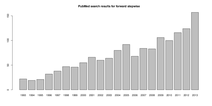
As a classical method dating back about half a century (see Hocking (1976) for a review), forward stepwise regression has not received much attention in recent years in the theoretical statistics community. But it continues to be widely used by practitioners. For example, search results on PubMed for forward stepwise, summarized in Figure 1, show that many recent papers mention the method and there is an increasing trend over time. Its popularity among researchers continues despite the fact that it invalidates inferences using the standard $\chi^{2}$ or $F$-tests.

Some attempts to address this issue include Monte Carlo estimation of tables of adjusted $F$-statistic values (Wilkinson and Dallal, 1981), and permutation statistics (Forsythe et al., 1973). Aside from the works this paper is based on, there have been other recent attempts to do inference after model selection. Most of these make use of subsampling (Meinshausen and Bühlmann, 2010) or data splitting (Wasserman and Roeder, 2009). Our approach allows use of the full data and does not require the extra computation involved in subsampling. Before describing the full approach we first introduce notation and specify our implementation of forward stepwise, which is slightly different from the most commonly used versions.

We allow forward stepwise selection to add groups of variables in each step, not only in the case of dummy variable encoding for categorical variables but also for any grouping purpose. For example, groups of variables may be pre-designated factors such as expression measurements for all genes in a single functional pathway. To emphasize this we use $g,h$ as covariate indices rather than the usual $i,j$ throughout. Since single variables can be considered groups of size 1, this includes non-grouped situations as a special case.

Let $y\in\mathbb{R}^{n}$ be $n$ i.i.d. measurements of the outcome variable. Let an integer $G\geq 2$ be the number of groups of explanatory variables. For each $1\leq g\leq G$ the design matrix encoding the $g$th group is the $n\times p_{g}$ matrix denoted $X_{g}$, where $p_{g}$ is the number of individual variables or columns in group $g$. When a group encodes a categorical variable as indicators for the levels of that variable, by default we use the full encoding with a column for every level. Although this introduces collinearity, our method does not require the design matrix to have full rank.

Denote by $p=\sum_{g=1}^{G}p_{g}$ the total number of individual variables, so $p=G$ in the case where all groups have size 1. Let $X$ be the matrix constructed by column-binding the $X_{g}$, that is

$$X=\begin{pmatrix}X_{1}&X_{2}&\cdots&X_{G}\end{pmatrix}$$

We also allow weights $w_{g}$ for each group. These weights act like penalties or costs, so increasing $w_{g}$ makes it more difficult for the group $X_{g}$ to enter the model. The modeler can choose weights arbitrarily for calibration purposes, but throughout we set them all constant (equal to 1) and normalize groups by the Frobenius norm of their corresponding submatrices.

With each group we associate the $p_{g}\times 1$ coefficient vector $\beta_{g}$, and write $\beta$ for the $p\times 1$ vector constructed by stacking all of the $\beta_{g}$ in order. Finally, our model for the response is

$$y =X\beta+\sigma\epsilon$$ (1)

$$=\sum_{g=1}^{G}X_{g}\beta_{g}+\sigma\epsilon$$

where $\epsilon$ is noise. We assume Gaussian noise $\epsilon|X\sim N(0,\Sigma)$ with known covariance matrix $\Sigma$.

The model (1) is underdetermined when $p>n$. In such cases it still may be possible to estimate $\beta$ well if it is sparse–that is, if it has few nonzero entries. In the rest of this paper we refer to variable groups $X_{g}$ as noise groups if $\beta_{g}$ is a zero vector and as true or signal groups if $\beta_{g}$ has any nonzero entries. We refer to the number of such nonzero groups as the sparsity of the model, and denote this $k:=\#\{g:\beta_{g}\neq 0\}$. With this notation we are now ready to describe our procedure concretely.

2.2 Description of the forward stepwise algorithm

First, the user must specify the maximum number of steps allowed, which we denote steps. To enable $T\chi$ statistic computations, steps should be at most $\min(n,G)-1$, but it is computationally desirable to set it as low as possible while safely larger than the sparsity of $\beta$. Then forward stepwise may recover all the nonzero coefficients of $\beta$ and terminate without performing much additional computation. Of course the sparsity is usually unknown, so this requires guesswork. In our implementation we treat the active set $A$ as an ordered list to easily track the order of groups entering the model.

Algorithm 1 Forward stepwise variant with groups and weights

0:  An $n$ vector $y$ and $n\times p$ matrix $X$ of $G$ variable groups with weights $w_{g}$

0:  Ordered active set $A$ of variable groups included in the model at each step

1:  $A\leftarrow\emptyset$, $A^{c}\leftarrow\{1,\ldots,G\}$, $r_{0}\leftarrow y$

2:  for $s=1$ to $steps$ do

3:     $g^{*}\leftarrow\mathop{\mathrm{argmax}}_{g\in A^{c}}\{\lVert X_{g}^{T}r_{s-1}\rVert_{2}/w_{g}\}$

4:     $P_{g^{*}}\leftarrow I_{n\times n}-X_{g^{*}}X_{g^{*}}^{\dagger}$

5:     $A\leftarrow A\cup\{g^{*}\}$, $A^{c}\leftarrow A^{c}\backslash\{g^{*}\}$

6:     for all $h\in A^{c}$ do

7:        $X_{h}\leftarrow P_{g^{*}}X_{h}$

8:     end for

9:     $r_{s}\leftarrow P_{g^{*}}r_{s-1}$

10:  end for

11:  return  $A$

The active set $A$ contains variable groups chosen to be included in the model. Fitting $\hat{\beta}$ can be done by tracking the individual fits and projections, or by simply fitting a linear model on the submatrix of $X$ corresponding to $A$. Note that other implementations of forward stepwise use different criteria for choosing the next variable to add, such as the correlation with the residual. Since we do not renormalize the columns after projecting the covariates (lines 6 to 8 above), and since we have weights, we are generally not computing correlations unless the design matrix is orthogonal and all weights are 1. We could renormalize the columns, though we choose not to. There are advantages and disadvantages to both criteria which we do not discuss. Our choice was motivated by the group LASSO result in Taylor et al. (2013), but we believe other criteria can be handled with appropriate modifications. We now use forward stepwise to refer specifically to Algorithm 1 unless otherwise specified.

2.3 Performance of forward stepwise

Among model selection procedures, forward stepwise is one which performs variable selection: from a potentially large set of variables it chooses a subset to include in the model. The most ambitious form of variable selection is “best-subset” selection, a procedure which picks the best model among all $2^{G}$ subsets of the $G$ possible groups. This exhaustive search is computationally infeasible when $G$ is large, and when possible it still runs the risk of over-fitting unless model complexity is appropriately penalized (as in (2) below). Forward stepwise produces a much smaller set of potential models, with cardinality at most steps (which, recall, is less than $\min(n,G)$). However it is a greedy algorithm, so the set of models it produces may not contain the best possible model. This is an inherent shortcoming of forward stepwise procedures and should be kept in mind when choosing between model selection methods.

So far we have left open the question of choosing among the models in the forward stepwise sequence, i.e. when to stop stepping forward. Some approaches for this problem can be posed as optimization criteria which stop at the step minimizing

$$\frac{1}{2}\|y-X\beta_{s}\|_{2}^{2}+\lambda\mathcal{P}(\beta_{s})$$ (2)

where we have written $\{\beta_{s}:s=1,\ldots,steps\}$ as the sequence of models output by forward stepwise. The function $\mathcal{P}(\beta)$ is a penalty on model complexity usually taken to be the number of nonzero entries of $\beta$. Proposals for $\lambda$ include 2 ($C_{p}$ of Mallows (1973), AIC of Akaike (1974)), $\log(n)$ (BIC of Schwarz (1978)), and $2\log(p)$ (RIC of Foster and George (1994)). Stopping rules based on classical test statistics have also been used, so it is natural to consider using the new test statistics of Lockhart et al. (2013) or Taylor et al. (2013) to choose a model. Grazier G’Sell et al. (2013) examined some stopping rules using the asymptotic $p$-values of Lockhart et al. (2013) and showed their stopping rules control false discovery rate–the expected proportion of noise variables among variables declared significant (Benjamini and Hochberg, 1995). We explore this further in Section 4.

Although forward stepwise is a greedy algorithm producing a potentially sub-optimal sequence of models, under favorable conditions it can still perform well. There is a subset of the compressed sensing literature (Donoho et al., 2006; Cai and Wang, 2011) dedicated to forward stepwise (often referred to in that literature as Orthogonal Matching Pursuit or OMP). Typical results from these works establish that forward stepwise can exactly select the true model under some stringent conditions involving quantities like the sparsity of the true model and the coherence of the design matrix. The coherence $\mu(X)$ of a matrix $X$ with columns scaled to have unit 2-norm is defined as

$$\mu:=\mu(X)=\max_{i\neq j}\{|\langle X_{i},X_{j}\rangle|\}$$ (3)

Denoting $k$ as the sparsity of $\beta$, the literature establishes that if $k<(1/\mu+1)/2$ and the nonzero coefficients of $\beta$ are sufficiently large then forward stepwise recovers $\beta$ with high probability. The coherence condition is necessary to guarantee exact recovery (Cai et al., 2010) in the sense that it is possible to construct counterexamples with $k=(1/\mu+1)/2$. We refer the reader to Donoho et al. (2006); Cai and Wang (2011) for details. For our purposes the conditions required to guarantee exact recovery are usually too stringent. Simulations show empirically that forward stepwise can work well even when it is not working perfectly, and that it does so under a wide range of conditions.

(a) Categorical designs

(b) Gaussian designs

Figure 2: For various sparsity levels $k$, the True Positive Proportion of the model selected by forward stepwise at $k$ steps. The left panel shows the results of the simulation using a categorical design consisting of 200 binary factors. The right panel shows the results with design matrices of Gaussian entries. Plotted in green are the TPP (dashed line) and median model sizes (top) for models chosen by BIC, and in purple the same are shown (dot-dash line, bottom) for RIC.

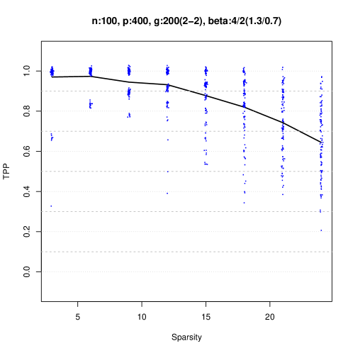
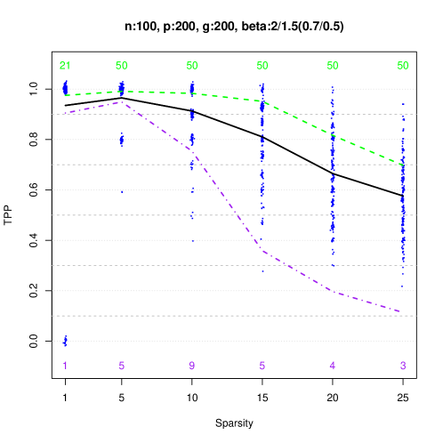
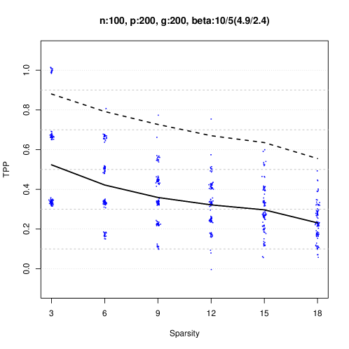
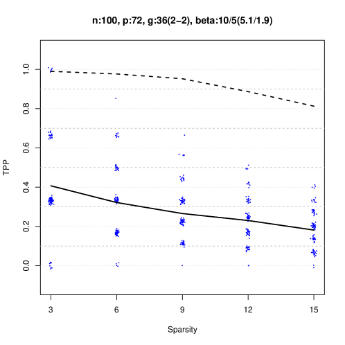
For various sparsity levels $k$, we applied Algorithm 1 to various data sets with steps set to $k$. In the resulting active set $A_{k}$, the number of true variables divided by $k$ is the $k$-True Positive Proportion ($k$-TPP):

$$k\text{-TPP}=\frac{\#\left\{g:g\in A_{k},\beta_{g}\neq 0\right\}}{k}.$$

Since we know $k$ in the simulations we can use $k$-TPP as a measure of how well forward stepwise is performing. When it is close to 1 we are recovering most of the true variables before including false ones. In our simulations nonzero coefficients have magnitudes in a range of multiples of $\gamma:=\sqrt{2\log(G)/n}$, e.g. in $[1.4\gamma,1.6\gamma]$. Results are shown in Figure 2. After computing the coherence of these design matrices, some calculations show the required sparsity level to guarantee exact recovery in these situations is about 2 or smaller, and the required nonzero coefficient magnitude is likely in the range of 10 to 100 times $\gamma$. These simulations are far from the stringent conditions required by theory to guarantee perfect recovery, but the performance, while not perfect, may still be good enough for some purposes. Finally, to serve as a comparison with existing commonly used model selection procedures, in Figure 2(b) we show in green the TPP and median model sizes for models chosen by the step function in R using the BIC criterion, and the same for RIC are plotted in purple.

3 Significance testing with model selection

3.1 Background

In the ordinary least squares setting, a significance test for a single variable can be conducted by comparing the drop in residual sums of squares (RSS) to a $\chi^{2}_{1}$ distribution. Similarly, when adding a group of $k$ variables we can compare the drop in RSS to a $\chi^{2}_{k}$ random variable. This generally does not work when the group to be added has been chosen by a method that uses the data (Olshen, 1973), and in particular it fails for forward stepwise procedures adding the “best” (e.g. most highly correlated) predictor in each step. In that case, the drop in RSS does not match its theoretical null distribution even when the null hypothesis is true. Lockhart et al. (2013) introduced a new test statistic based on the knots in the LASSO solution path. They derived a simple asymptotic null distribution, proved a type of convergence under broad “minimum growth” conditions, and demonstrated in simulations that the test statistic closely matches its asymptotic distribution even in finite samples. That work marked an important advance in the problem of combining inference with model selection. Taylor et al. (2013) extended that work to the group LASSO (Ming and Lin, 2005) and other problems, and modified the test statistic to one with an exact finite sample distribution under the global null hypothesis.

To describe the previous work we require some facts about the solution path of the LASSO. Recall the LASSO estimator is given by

$$\hat{\beta}(\lambda)=\mathop{\mathrm{argmin}}_{\beta\in\mathbb{R}^{p}}\frac{1}{2}\|y-X\beta\|_{2}^{2}+\lambda\|\beta\|_{1}$$ (4)

The following facts are summarized in Lockhart et al. (2013); Tibshirani (2012).

• The vector valued function $\hat{\beta}(\lambda)$ is a continuous function of $\lambda$. For the LASSO path, the coordinates of $\hat{\beta}(\lambda)$ are piecewise linear with changes in slope occurring at a finite number of $\lambda$ values referred to as knots.

• The knots depend on the data and are usually written in order $\lambda_{1}\geq\lambda_{2}\geq\cdots\geq\lambda_{r}\geq 0$.

Assuming groups of size one and $\Sigma=\sigma^{2}I$, the covariance test is given at the first step by

$$T_{1}=\frac{\lambda_{1}(\lambda_{1}-\lambda_{2})}{\sigma^{2}}\overset{n,p\to\infty}{\to}\text{Exp}(1).$$ (5)

This is a hypothesis test for including the first variable in the LASSO path, with large values of the test statistic being evidence against the global null. In Taylor et al. (2013) it is pointed out

$$\exp\left(-\frac{\lambda_{1}(\lambda_{1}-\lambda_{2})}{\sigma^{2}}\right)\approx\frac{1-\Phi(\lambda_{1}/\sigma)}{1-\Phi(\lambda_{2}/\sigma)}\overset{D}{=}\text{Unif}([0,1]).$$ (6)

The right hand side has an exact, finite sample null distribution. Further, this new statistic can be understood as the survival function of $\lambda_{1}=\|X^{T}y\|_{\infty}$ conditional on which variable achieves $\lambda_{1}$ as well as its sign. The limiting results about later steps in Lockhart et al. (2013) can be interpreted as recursively applying $T_{1}$ to the variables that had not previously been selected by LARS. In forward stepwise with groups of size 1, we recursively apply the right hand side test statistic in the same manner. With larger groups, we use an analogous test statistic to the right hand side of (6). The test statistic is presented as an example in Taylor et al. (2013) though we re-derive it here in simpler form. The test draws inspiration from the group LASSO.

The group LASSO estimator (Ming and Lin, 2005; Bakin et al., 1999), a generalization of the LASSO, is a solution to the following penalized least-squares convex problem

$$\hat{\beta}_{\lambda}=\mathop{\mathrm{argmin}}_{\beta\in\mathbb{R}^{p}}\frac{1}{2}\|y-X\beta\|_{2}^{2}+\lambda{\cal P}(\beta)$$ (7)

with the group penalty

$${\cal P}(\beta) =\sum_{g=1}^{G}w_{g}\|\beta_{g}\|_{2}$$ (8)

The parameter $\lambda\geq 0$ enforces sparsity in groups: for large $\lambda$ most of the $\beta_{g}$ will be zero vectors. The weights $w_{g}$ are usually taken to be $\sqrt{p_{g}}$ to normalize the penalty across groups with different sizes. This can also be accomplished by scaling the corresponding submatrices by their Frobenius norms and setting all weights equal. Note that this includes the usual LASSO estimator as a special case when all groups are of size 1, since then the penalty term is the $\ell_{1}$-norm of $\beta$. The solution path of the group LASSO has similar properties to the LASSO case, however it is not generally piecewise linear.

For sufficiently large $\lambda$ the solution to (7) is forced to be zero. The smallest such $\lambda$ is denoted

$$\lambda_{1} =\inf\{\lambda\geq 0:\hat{\beta}_{\lambda^{\prime}}=0\text{ for all }\lambda^{\prime}>\lambda\}$$ (9)

For the group LASSO this is explicitly computable by

$$\lambda_{1}^{\text{group}}=\max_{g}\frac{1}{w_{g}}\|X_{g}^{T}y\|_{2}.$$ (10)

The value above is also the dual norm of the penalty (8) hence it can be expressed as

$$\lambda_{1}^{\text{group}}=\frac{1}{w_{g^{*}}}\eta_{g^{*}}^{T}X_{g^{*}}^{T}y.$$ (11)

where $g^{*}$ is the group that achieves the maximum and $\eta_{g^{*}}=X_{g^{*}}^{T}y/\|X_{g^{*}}^{T}y\|_{2}$ is the unit vector that achieves the norm $\|X_{g^{*}}^{T}y\|_{2}$. One of the key conceptual points about our test is that it conditions on both the maximizer $g^{*}$ and on the unit vector $\eta_{g^{*}}$. Most of the $p$-value computations will be done in terms of these quantities.

3.2 Quadratic framework and derivation of test statistic

In this section we derive the new $p$-value and describe how to compute it. First we give a brief summary of what follows; readers not interested in the full derivation can skip the rest of this section after they understand the summary. The event $E_{g}$ that forward stepwise Algorithm 1 selects a given group $g$ is equivalent to a set of quadratic inequalities involving $y$ (see (13) below). To derive a statistic related to the group $g$ being included, we choose a direction vector $\eta(g)$ in the relevant direction and study the distribution of $\eta(g)^{T}y$ restricted to the event $E_{g}$. In Figure 3 below the event $E_{g}$ is the shaded region, and the direction $\eta$ determines a slice through this event. Finally, we solve for the amounts $t$ by which $y$ can be translated in the directions $\pm\eta$ and still satisfy the constraints imposed by $E_{g}$. These are the points where the slice intersects the boundary of $E_{g}$. Let $M\subset\mathbb{R}$ be the set of $t$ such that $y+t\cdot\eta\in E_{g}$. With all of these quantities and a little more work we find that the observed norm $\|X_{g}^{T}y\|_{2}$ has a $\chi$ distribution truncated to the set $M$, and with a computable scale parameter. Applying the appropriate CDF transform (19) with these quantities yields our $p$-value.

We now give the full derivation of the $p$-value, beginning with a previous work and then extending the framework there to the setting with groups. The approach to post-selection inference in Lee et al. (2013) describes the selection event for the LASSO as a convex polytope satisfying a list of affine constraints. If all groups are of size 1, then the event that we observe a given set of variables in the forward stepwise path (with their signs as they enter) would similarly be given by a set of affine inequalities. After selection, exact inference for a (randomly) chosen contrast $\eta(y)^{T}\mu$ of the mean vector $\mu$ could then be accomplished by analyzing the conditional distribution

$$y\sim N(\mu,\sigma^{2}I)\bigl{|}Ay\leq b.$$ (12)

See Lee et al. (2013); Taylor et al. (2014) for further details on this approach.

However, with group sizes larger than 1, the event that the first group chosen $g^{*}(y)$ is equal to some fixed group $g$ is no longer given by a set of affine constraints. Rather, considering line 3 of Algorithm 1, we see

$$\{g^{*}(y)=g\} =\{\|X_{g}^{T}y\|_{2}/w_{g}\geq\|X_{h}^{T}y\|_{2}/w_{h},\ \forall h\neq g\}$$ (13)

$$=\{y^{T}(X_{g}^{T}X_{g})y/w_{g}^{2}-y^{T}(X_{h}^{T}X_{h})y/w_{h}^{2}\geq 0,\ \forall h\neq g\}$$

Hence, our selection event can be expressed as the intersection of a list of quadratic inequalities. This non-affine selection event is stylized in Figure 3. In the rest of this section, we consider an arbitrary selection procedure $S$ that returns one of a set of possible outcomes $s\in{\cal S}$ determined by a set of quadratic inequalities. That is, for all possible outcomes $s\in{\cal S}$ there is a set of indices $I(s)$ such that

$$\{S(y)=s\}=\cap_{i\in I(s)}\{y:y^{T}Q_{i}y+a_{i}^{T}y\leq b_{i}\}.$$ (14)

The quadratic forms are not assumed non-negative definite, but we can, without loss of generality assume they are symmetric. As in Lee et al. (2013) we will be interested in some randomly chosen contrast $\eta(s)^{T}\mu$. In our grouped selection procedure, the selection rule is $S(y)=g^{*}(y)$ and the value of $\eta$ on $\{g^{*}=g\}$ is

$$\eta(s)=\eta(g)=\frac{X_{g}^{T}y}{\|X_{g}^{T}y\|_{2}}.$$

This choice of $\eta$ reflects our goal of calculating a $p$-value for inclusion of the variable $g^{*}$ chosen by forward stepwise. Note that for each fixed $g$ and any $\eta\in\mathbb{R}^{g}$ with $\|\eta\|_{2}=1$, the event

$$\left\{y:\frac{X_{g}^{T}y}{\|X_{g}^{T}y\|_{2}}=\eta\right\}=\left\{y:\|X_{g}^{T}y\|^{2}_{2}\leq(X_{g}\eta)^{T}y\right\},$$

is defined by another quadratic inequality that can be appended to $I(s)$.

Having fixed $\eta$, we proceed to study this contrast by slicing through the selection event along a ray with direction $\eta$ that passes through $y$. That is, we need to find

$$\left\{t\in\mathbb{R}:S(y+t\cdot\eta)=s\right\}$$

$$\qquad=\cap_{i\in I(s)}\left\{t\in\mathbb{R}:(y+t\cdot\eta)^{T}Q_{i}(y+t\cdot\eta)+a_{i}^{T}(y+t\cdot\eta)\leq b_{i}\right\}.$$

Figure 3: A quadratic selection event, given by the intersection of a list of quadratic inequalities. The selection event and chosen contrast $\eta$ determine a slice through the event with computable limits where the boundary of the event is reached. Note that the event need not be simply connected.

The slice for any particular inequality is

$$\hbox to0.0pt{$\displaystyle\left\{t\in\mathbb{R}:(y+t\cdot\eta)^{T}Q_{i}(y+t\cdot\eta)+a_{i}^{T}(y+t\cdot\eta)\leq b_{i}\right\}$\hss}$$ (15)

$$\qquad=\left\{t\in\mathbb{R}:t^{2}\cdot(\eta^{T}Q_{i}\eta)+t\cdot(2y^{T}Q_{i}\eta+a_{i}^{T}\eta)+y^{T}Q_{i}y+a_{i}^{T}y-b_{i}\leq 0\right\}$$

This can be computed explicitly, and results in either the empty set, a single interval (possibly infinite) or the union of two disjoint infinite intervals. The intersection over all $I(s)$ is therefore also computable, yielding a form for the slice

$$\{g^{*}(y)=g,\eta(g^{*}(y))=\eta\}.$$ (16)

In Figure 3, for every $\eta$, the slice (16) is a function of $P_{\eta}^{\perp}y$. This amounts to a proof of the following lemma.

Lemma 1.

Suppose $S$ is a selection procedure, i.e. a map $S:\mathbb{R}^{n}\mapsto{\cal S}$ such that for each $s\in S$ (14) holds and we are given a matrix valued function $X_{s}\in\mathbb{R}^{n\times p(s)}$ of rank $k(s)$. Then, for every $\eta_{s}\in\mathbb{R}^{p(s)}$ with $\|\eta_{s}\|_{2}=1$, the slice

$$\left\{t:S(y+t\cdot\eta_{s})=s,\frac{X_{s}^{T}y}{\|X_{s}^{T}y\|_{2}}=\eta_{s}\right\}$$ (17)

can be described by a finite union of closed intervals whose endpoints are functions of $(P_{s}^{\perp}y,(P_{s}-(X_{s}\eta_{s})(X_{s}\eta_{s})^{T})y)$ where $P_{s}^{\perp}$ is projection on the orthogonal column space of $X_{s}$.

Denote the set (17) by $E(s,\eta_{s},P_{s}^{\perp}y,(P_{s}-X_{s}\eta_{s}(X_{s}\eta_{s})^{T})y)$ and also define

$$E_{+}(s,\eta_{s},P_{s}^{\perp}y,(P_{s}-X_{s}\eta_{s}(X_{s}\eta_{s})^{T})y)$$

$$\qquad=\left\{y+t\cdot\eta_{s}:S(y+t\cdot\eta)=s,\frac{X_{s}^{T}y}{\|X_{s}^{T}y\|_{2}}=\eta_{s}\right\}$$

We now present an explicit algorithm for computing this slice in quadratic selection procedures.

Algorithm 2 Truncation interval for quadratic decisions

0:  Response $y$, state $s$ list of quadratic inequalities $\{Q_{i},a_{i},b_{i}:i\in I(s)\}$, direction of interest $\eta$ with $\|\eta\|_{2}=1$.

0:  The set $\{t:(y+t\cdot\eta)^{T}Q_{i}(y+t\cdot\eta)+a_{i}^{T}(y+t\cdot\eta)\leq b_{i}\ \forall i\in I(s)\}$.

  Initialize interval: $M=(-\infty,\infty)$, $U=-\infty,L=\infty$

  for $i$ in $I(s)$ do

     $a=\eta^{T}Q_{i}\eta,b=2y^{T}Q_{i}\eta+a_{i}^{T}\eta,c=y^{T}Q_{i}y+a_{i}^{T}y-b_{i}$

     if $a\neq 0$ then

        if $b^{2}-4ac>0$ then

           Stop: $y$ does not satisfy inequalities!

        else if $a>0$ then

           $M\leftarrow M\cap[(-b-\sqrt{b^{2}-4ac})/2a,(-b+\sqrt{b^{2}-4ac})/2a]$;

        else if $a<0$ then

           $L\leftarrow\min(L,(-b-\sqrt{b^{2}-4ac})/2a)$,

           $U\leftarrow\max(U,(-b+\sqrt{b^{2}-4ac})/2a).$;

        end if

     else

        if $b>0$ then

           $M\leftarrow M\cap(-\infty,-c/b]$;

        else if $b<0$ then

           $M\leftarrow M\cap[-c/b,\infty)$;

        else if $c>0$ then

           Stop: $y$ does not satisfy inequalities!

        end if

     end if

  end for

  return  $(M\cap(L,U)^{c})+\eta^{T}y.$

In turn, this allows us to derive a test statistic to test the hypothesis $H_{0,s}:X_{s}^{T}\mu=0$ conditional on $s$ being selected.

Lemma 2.

For $y\sim N(0,\sigma^{2}I)$, conditional on the event

$$H_{0,s}\cap E_{+}(s,\eta_{s},P_{s}^{\perp}y,(P_{s}-\eta_{s}\eta_{s}^{T})y)$$

we have the following truncated $\chi$ distributional result

$$(X_{s}\eta_{s})^{T}y\overset{D}{=}\theta_{s}\chi_{k(s)}|(X_{s}\eta_{s})^{T}E_{+}(s,\eta_{s},P_{s}^{\perp}y,(P_{s}-\eta_{s}\eta_{s}^{T})y)$$ (18)

where the vertical bar $|$ here denotes restriction to an interval, and the scale is given by

$$\theta_{s}=\sigma\frac{y^{T}P_{s}y}{y^{T}X_{s}X_{s}^{T}y}.$$

Proof: For any fixed $s$, decompose $y$ as

$$(Z^{\perp}_{s},Z_{s})=(P_{s}^{\perp}y,X_{s}^{T}y).$$

Under $H_{0,s}:X_{s}^{T}\mu=0$, the density of $Z_{s}$ can be written as

$$(2\pi\Sigma_{s}\sigma^{2})^{-k(s)/2}\exp\left(-\frac{1}{2\sigma^{2}}z^{T}\Sigma_{s}^{-1}z\right)$$

with $\Sigma_{s}=X_{s}^{T}X_{s}$. Transforming to polar coordinates $(R,U)$ yields a density

$$(2\pi\Sigma_{s}\sigma^{2})^{-k(s)/2}r^{k(s)-1}\exp\left(-\frac{r^{2}}{2\sigma^{2}}u^{T}\Sigma_{s}^{-1}u\right),\qquad r\geq 0,\|u\|_{2}=1.$$

Conditioning on $U$ shows that $R=\|X_{s}^{T}y\|_{2}|U$ has distribution proportional to a $\chi_{k(s)}$. Finally, observe that the scale of the $\chi$ above is given by $\theta_{s}$. ∎

3.3 The $T\chi$ test statistic

With Lemma 2 and Algorithm 2 we are finally ready to define our test statistic, which we term the truncated $\chi$ test statistic, denoted $T\chi$. This statistic is determined by a degrees of freedom parameter $r$ as well as a truncation set $M\subset\mathbb{R}$, a scale parameter $\theta$ and an observed value $t$. The test statistic is given by the survival function of a $\chi_{r}$ random variable truncated to the set $M$ evaluated at our observed norm $\|X_{g}^{T}y\|_{2}$ (after scaling by the appropriate scale $\theta$).

$$T\chi(t,r,\theta,M)=\frac{\int_{M/\theta\cap[t/\theta,\infty)}F_{\chi_{r}}(dz)}{\int_{M/\theta}F_{\chi_{r}}(dz)}.$$ (19)

For simplicity we always use this distributional transform rather than reporting the observed values of $(t,r,\theta,M)$. Hence, $T\chi$ itself is our $p$-value, with

$$T\chi\sim\text{Unif}([0,1])$$

under the global null.

After adding the first group in forward stepwise and computing the $T\chi$ $p$-value, we orthogonalize the response $y$ and all remaining groups with respect to the group just added. This imposes further constraints that in principle should be used when computing $p$-values at subsequent steps. For now we ignore these constraints and iterate the global null test, but work on incorporating all known constraints is ongoing. We believe that the effect of not tracking all constraints is what causes the nominal $p$-value to be increasingly stochastically larger than uniform further down the forward stepwise path (as can be seen in Figure 4), and only truly uniform at the first step where all remaining variables are noise.

For an alternate derivation that follows more closely Taylor et al. (2013), and an algorithm that includes weights and an arbitrary (known) covariance matrix $\Sigma$ see Appendix A.

4 Simulations

To study the behavior of the $T\chi$ test after taking steps in the forward stepwise path and to understand its power to detect various departures from the global null we conduct simulations in a wide variety of settings including both $p>n$ and $p<n$ problems. We performed simulations with several classes of random design matrices including Gaussian and categorical, and with fixed categorical designs from the HIV data set of Section 5.3. Gaussian design matrices were generated either independently or with some global correlation $\rho>0$ between all pairs of columns. Categorical matrices were generated by first choosing a vector of probabilities for a given variable from a Dirichlet prior, and then sampling category levels with that vector of probabilities. Resampling was used to ensure the minimum number of observations in any level was at least five. Finally, categorical variables were encoded as groups of 0-1 vectors using the full encoding.

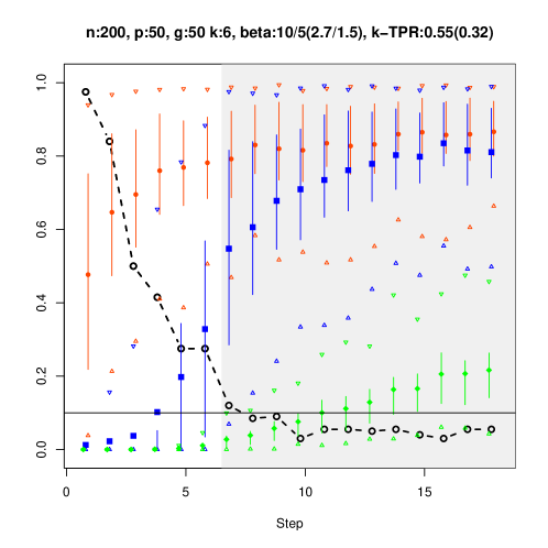
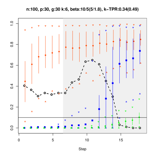
Since we are interested in variable selection we generate signals with nonzero coefficients on the scale of $\gamma:=\sqrt{2\log(G)/n}$, where recall $G$ is the number of groups. Coefficients within a nonzero group have roughly the same magnitude and are normalized so that $\|\beta_{g}\|_{2}$ has scale $\gamma$ independently of $p_{g}$. The magnitudes for different nonzero groups range from a lower limit times $\gamma$ to an upper limit times $\gamma$. In text above each plot, the limits are listed next to “beta” and the numbers in parentheses are the largest and smallest 2-norms of nonzero coefficient groups respectively. Each plot also displays the number of observations or rows, $n$, the number of columns, $p$, the number of groups, $g$, and the largest and smallest group sizes in parentheses if the groups are not all size 1. The number of nonzero groups, $k$, is also displayed graphically by shading with the portion of the plot showing steps after $k$ shaded gray. The proportion of truly nonzero groups recovered in the first $k$ steps is denoted $k$-TPP, where recall $k$ is the number of truly nonzero groups.

(a) Gaussian with correlations

(b) Gaussian with groups

Figure 4: Forward stepwise with $T\chi$ simulation results. Dashed line is the local True Positive Rate at each step averaged over 400 simulation realizations. Vertical lines are boxplots of $p$-values marginally at each step, with red computed using $T\chi$ on a null model, blue using $T\chi$ on a sparse alternative model, and green using $\chi^{2}$ on the same. The shaded region indicates the sparsity of the alternative. Left panel shows results for Gaussian design matrices with equicorrelation $\rho=0.2$ and equicorrelated noise with correlation 0.1. Right panel shows results for an independent Gaussian design with groups of sizes 5 and 10.

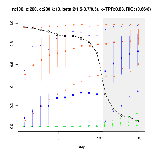
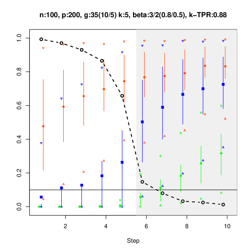
We show two types of plots, one containing the same information as in Figure 2. The other plots each show a scenario with a fixed sparsity level and contain the following information. The horizontal axis is the step index for forward stepwise. The dashed line shows the proportion of iterations where a truly nonzero variable was added to the model at that step. Solid verticle lines are essentially narrow boxplots, showing the middle 50% of $p$-values calculated at that step with circular points in these lines as the average and triangles showing the 95% and 5% quantiles. Different color verticle lines represent the following: red are calculated using the $T\chi$ $p$-value on a null model with no nonzero groups, blue are calculated using the $T\chi$ $p$-value on the non-null model, and green calculated on the non-null model using the usual $\chi^{2}$ significance test.

(a) Real data categorical design

(b) Simulated categorical design

Figure 5: As in Figure 4. The left panel shows results for a categorical design taken from a real data set. The right panel shows results for categorical matrices with all categories having 5 levels. The null cases being larger than uniform are likely the result of numerical error as these problems are poorly conditioned.

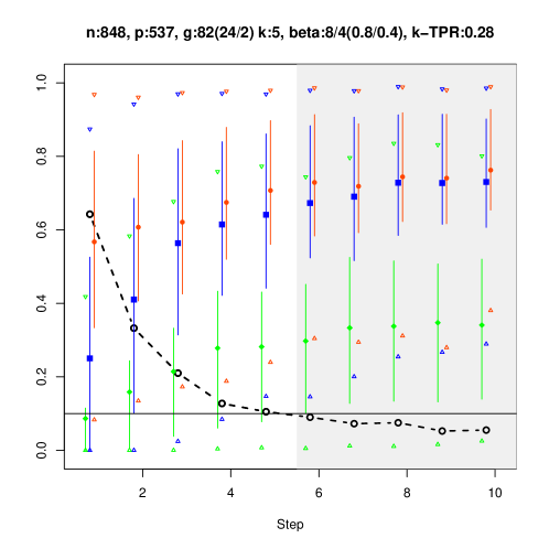
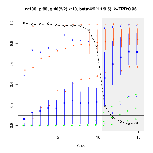
The performance of forward stepwise in these plots is characterized by how close the dashed line is to a step function. If forward stepwise finds all truly nonzero variables first this line will be close to 1 until the step index reaches $k$ and then it will be close to 0. When this is the case, the $T\chi$ $p$-value tends to be small while forward stepwise is selecting truly nonzero variables, uniform on the step where the dashed line goes to 0, and then progressively larger afterward. A reasonable stopping rule based on this behavior is to pick the model including all variables up to and including the last one with a significant $p$-value. We call this the last stopping rule, and it selects the first $\hat{k}_{\textit{last}}$ variables in the forward stepwise path where, if $p_{j}$ denotes the $T\chi$ $p$-value calculated at the $j$-th step, then

$$\hat{k}_{\textit{last}} =\max\{j\leq steps:p_{j}<\alpha\}.$$ (20)

To test this stopping rule we compare it with several others which we now describe. The oracle stopping rule assumes knowledge of the sparsity $k$ and always picks the first $k$ variables. The first rule stops immediately before the first variable to yield a $p$-value larger than $\alpha$, and since this requires rejection of the global null in order to include the first variable it controls the family-wise error rate. However it does not seem to have good power. The forward stopping rule is defined in Grazier G’Sell et al. (2013) and has the desirable property that it controls the false discovery rate. Finally, RIC and BIC are the risk inflation criterion and Bayesian information criterion described in Section 2.3. Tables 2 and 3 show simulation results with $\alpha=0.1$. To summarize these results, forward is the only rule which controls FDR, BIC selects models that are far too large, RIC has low FDR and good power when the sparsity is low, and last is comparable to RIC, with perhaps more power in the higher dimensional setting (and a correspondingly larger FDR when the signal is also weak).

p		50			500
k	rule	R	FDP	TPP	R	FDP	TPP
	oracle	10(0)	0.06(0.08)	0.94(0.08)	10(0)	0.16(0.18)	0.84(0.18)
	first	1.5(1.5)	0(0.03)	0.14(0.14)	2.1(1.8)	0.04(0.14)	0.2(0.17)
10	forward	0.7(0.5)	0(0)	0.07(0.05)	0.8(0.4)	0.01(0.11)	0.08(0.04)
	last	8.6(2)	0.03(0.06)	0.84(0.19)	9.4(2.5)	0.12(0.16)	0.82(0.22)
	RIC	9(2)	0.05(0.08)	0.85(0.19)	6.2(3.5)	0.09(0.15)	0.57(0.33)
	BIC	12(1.8)	0.17(0.11)	0.98(0.05)	50(0)	0.81(0.03)	0.94(0.13)
	oracle	15(0)	0.07(0.07)	0.93(0.07)	15(0)	0.4(0.22)	0.6(0.22)
	first	1.7(1.5)	0.01(0.09)	0.11(0.1)	2.3(1.8)	0.07(0.17)	0.14(0.11)
15	forward	0.8(0.4)	0.01(0.1)	0.05(0.03)	0.8(0.4)	0.04(0.2)	0.05(0.03)
	last	12.5(3.3)	0.04(0.06)	0.8(0.21)	11.4(4)	0.29(0.22)	0.53(0.25)
	RIC	11.2(4.1)	0.05(0.08)	0.71(0.27)	3.6(2.8)	0.11(0.2)	0.21(0.17)
	BIC	16.9(2.3)	0.14(0.09)	0.96(0.09)	50(0)	0.78(0.07)	0.73(0.23)

Table 2: Evaluation of model selection characteristics using several stopping rules. Here $n$ is fixed at 100, $p$ has 50 or 500 independent gaussian vectors, and the sparsity $k$ is set to 10 or 15. Nonzero coefficients have magnitudes in $[1.5\gamma,2\gamma]$ for $\gamma=\sqrt{2\log(p)/n}$. The average over 400 simulations of the selected model size (R), false discovery proportion (FDP), and true positive proportion (TPP) are shown with Monte Carlo standard errors in parentheses.

p		50			500
k	rule	R	FDP	TPP	R	FDP	TPP
	oracle	15(0)	0.18(0.09)	0.82(0.09)	15(0)	0.54(0.17)	0.46(0.17)
	first	1.1(1.1)	0(0.06)	0.07(0.07)	1.5(1.3)	0.08(0.22)	0.09(0.08)
15	forward	0.6(0.5)	0(0.05)	0.04(0.03)	0.7(0.4)	0.05(0.21)	0.05(0.03)
	last	6.3(3.7)	0.03(0.07)	0.4(0.23)	7.2(3.6)	0.28(0.25)	0.32(0.17)
	RIC	6.5(3.1)	0.06(0.1)	0.41(0.2)	2.4(1.8)	0.12(0.24)	0.14(0.11)
	BIC	14.2(2.9)	0.16(0.1)	0.79(0.15)	50(0)	0.84(0.05)	0.54(0.18)
	oracle	20(0)	0.17(0.08)	0.83(0.08)	20(0)	0.65(0.12)	0.35(0.12)
	first	1.3(1.2)	0.02(0.11)	0.06(0.06)	1.6(1.4)	0.12(0.26)	0.07(0.06)
20	forward	0.7(0.5)	0.02(0.13)	0.03(0.02)	0.7(0.4)	0.07(0.25)	0.03(0.02)
	last	7.7(4.3)	0.05(0.09)	0.36(0.2)	8.8(4.2)	0.41(0.23)	0.24(0.11)
	RIC	6.1(2.9)	0.05(0.11)	0.29(0.14)	2(1.5)	0.14(0.27)	0.08(0.07)
	BIC	17.2(3.9)	0.14(0.09)	0.74(0.16)	50(0)	0.84(0.05)	0.4(0.12)

Table 3: As in the previous table, but here the sparsity $k$ is set to 15 or 20 and nonzero coefficients have magnitudes in $[1.1\gamma,1.5\gamma]$ for $\gamma=\sqrt{2\log(p)/n}$.

5 Applications

We now turn to applying forward stepwise and examining the behavior of the $T\chi$ test in several unique settings, including a real data example.

5.1 Nonlinear regression with splines

(a) Power of forward stepwise with spline groups

(b) $T\chi$ $p$-values with spline groups

Figure 6: The first panel shows the power of forward stepwise in this setting for various sparsity levels, with the dashed line showing a liberal definition of power that allows mistakes when choosing between a non-zero spline group and its corresponding linear term. The second panel shows the $T\chi$ $p$-value marginally over each step, with red indicating the global null case, blue indicating a signal with $k=6$ nonzero groups, and green showing the nominal $\chi^{2}$ $p$-values also computed on the non-null case.

First we consider a simple extension of the usual linear regression setting to include nonlinear effects. Given a design matrix $X$, we augment this by adding additional columns given by nonlinear functions of the original covariates. Specifically, for each original covariate $X_{g}$ we compute a submatrix of spline basis vectors $X_{g}^{s}$. Adding these groups of spline basis vectors to the original design matrix yields a new design matrix

$$\tilde{X} =\begin{pmatrix}X_{1}&\cdots&X_{G}&X^{s}_{1}&\cdots&X^{s}_{G}\end{pmatrix}$$ (21)

with $\tilde{G}=2G$ groups. Thus, at each step the procedure chooses between including a linear effect for each covariate or including a full spline basis if the true relationship is nonlinear. For simplicity we assume the original groups are all size 1, and use the B-spline basis. In our simulations we generate original covariates uniformly in the interval [-1,1] and use cubic splines with boundary knots

$$X_{g} \sim\text{Unif}([-1,1]),\quad X_{g}^{s}=\text{CubicSplineBasis}(X_{g}).$$ (22)

Nonzero coefficients are split between original covariates and spline groups. Simulation results are shown in Figure 6. Note that the varying group sizes present some difficulty to forward stepwise, which tends to first try linear approximations to nonzero spline groups before adding the true spline group. In Figure 6(b) the average proportion of truly nonzero spline groups included in the first $k$ steps appears in parentheses next to the $k$-TPP (top right).

5.2 Glinternet for hierarchical interactions

In regression settings with many variables, choosing among models with pairwise interactions can drastically increase model complexity. Lim and Hastie (2013) propose a method called glinternet to reduce the statistical complexity of this problem. The method imposes a strong hierarchical constraint on interactions (similar to that in Bien et al. (2012)) where an interaction term can only be included if both its main effects are also included. They accomplish this by creating a design matrix with both main effects alone and also with groups including main effects with their first order interactions. Then they fit a group LASSO model with the expanded design matrix. Because interaction terms only appear in groups along with their respective main effects, the hierarchy condition holds for the fitted model. We now consider a related procedure as an example problem, but first modify their method to simplify some parts. Let the expanded design matrix be given by

$$\tilde{X}=\begin{pmatrix}X_{1}&\cdots&X_{G}&X_{1:2}&\cdots&X_{1:G}&X_{2:3}&\cdots&X_{(G-1):G}\end{pmatrix}$$ (23)

where $X_{g:h}$ is the submatrix encoding the interaction between $X_{g}$ and $X_{h}$. For example, if both of these are categorical variables, then $X_{g:h}$ consists of all $p_{g}p_{h}$ column multiples between columns in group $g$ and columns in group $h$. For example, if

$$X_{g}=\begin{pmatrix}X_{g1}&X_{g2}\end{pmatrix},\quad X_{h}=\begin{pmatrix}X_{h1}&X_{h2}\end{pmatrix}$$

are two categorical variables each with two levels, then

$$X_{g:h}=\begin{pmatrix}X_{g1}*X_{h1}&X_{g1}*X_{h2}&X_{g1}*X_{h1}&X_{g2}*X_{h2}\end{pmatrix}$$

where * denotes the pointwise product (Hadamard product) of vectors (the $i$th entry of $X_{g1}*X_{h1}$ is the $i$th entry of $X_{g1}$ times the $i$th entry of $X_{h1}$). For more details see Lim and Hastie (2013). Note that this expanded matrix has $\tilde{G}=G+\binom{G}{2}=O(G^{2})$ groups. We refer to the first $G$ of these as main effect groups and the remaining as interaction groups. Finally, instead of fitting a model by group LASSO, we use forward stepwise on the expanded design matrix and call the resulting procedure FS-glinternet. The overlapping groups still guarantee that our fitted model satisfies the strong hierarchy condition.

To demonstrate this method by simulation, we constructed signals which have the first $k/3$ main effects nonzero but with no interactions, and the remaining $2k/3$ nonzero main effects are matched to each other to form interactions. We also inflate each nonzero interaction coefficient to be larger than the corresponding main effect coefficients. This special case is favorable for our algorithm, but our purpose here is merely to demonstrate the flexibility of the hypothesis test and not to propose an optimal procedure for models with interactions.

Results are shown in Figure 7. The left panel shows average power of forward stepwise. Power is calculated using the group structure we impose, and not in terms of the original main effects and interactions. However, the dashed line shows a more forgiving definition of power where we are rewarded for discovering part of a nonzero group, i.e. for discovering only one main effect from a true interaction group. The proportion of nonzero interaction groups that were discovered in the first $k$-steps is shown in parentheses after the $k$-TPP (top right).

(a) Power of FS-glinternet procedure

(b) $T\chi$ $p$-values with FS-glinternet

Figure 7: The first panel shows the power of forward stepwise on the glinternet problem for various sparsity levels. The dashed line shows a more forgiving definition of power described in the section. The second panel shows the $T\chi$ $p$-value marginally over each step, with red indicating the global null case, blue indicating a signal with $k=6$ nonzero groups, and green showing the nominal $\chi^{2}$ $p$-values.

5.3 HIVdb data example

Rhee et al. (2006) use genomic information to predict efficacy of antiretroviral drugs in treating HIV. Quantitative measurements of drug response/resistance were regressed on categorical covariates encoding the presence and type of genetic mutations in certain regions of the HIV genome. We attempt a similar analysis using forward stepwise, and report the $T\chi$ $p$-value at each step. Categorical covariates are encoded as groups of dummy variables using the full encoding, and these groups are normalized by their Frobenius norm. We perform forward stepwise once for each drug response, restricting to the subset of the data with no missing values.

Figure 8: Forward stepwise results from PI dataset

Figure 9: Forward stepwise results from NRTI dataset

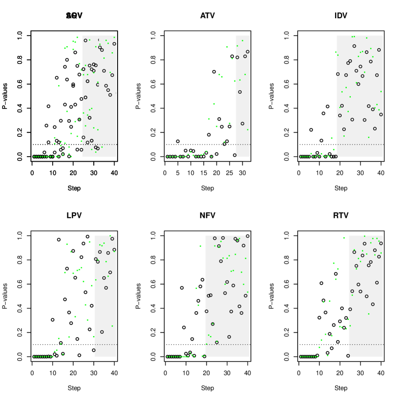
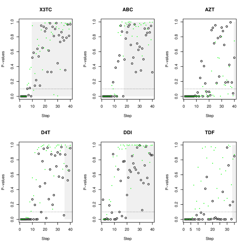
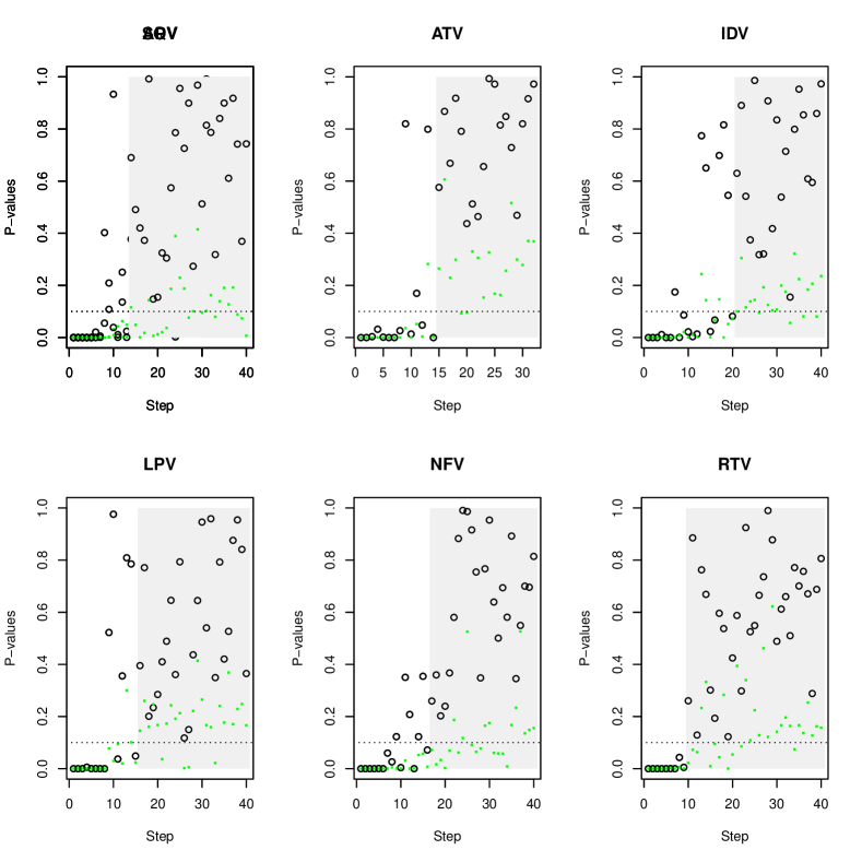
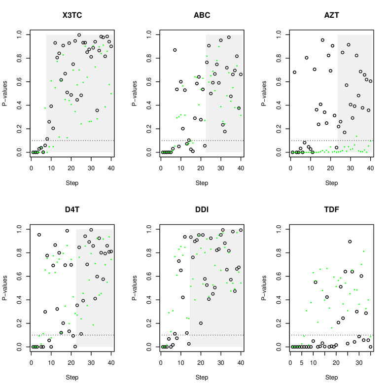
Results from two data sets are displayed in Figure 8 and Figure 9. The PI data contains protease inhibitor mutations, and the NRTI data contains nucleoside RT inhibitor mutations. Each panel shows results for a different drug, with $p$-values plotted by step in forward stepwise. The last stopping rule (20) is applied and the region of the plot corresponding to the chosen model is unshaded, with the remainder shaded. The first several chosen variables are shown in Tables 4 and 5.

Drug	n	G	$\hat{k}$	Selected variables
APV	768	82	24	P90 P46 P54 P84 P88 P32 P50 P76 P33 P10 P15 P82 …
ATV	329	71	27	P90 P54 P84 P50 P30 P32 P24 P76 P62 P46 P35 P88 …
IDV	827	82	18	P90 P46 P54 P84 P82 P62 P88 P73 P35 P50 P71 P24 …
LPV	517	76	30	P90 P54 P46 P84 P36 P82 P76 P47 P50 P10 P73 P33 …
NFV	844	82	19	P90 P46 P30 P54 P84 P36 P88 P73 P24 P82 P50 P71 …
RTV	795	82	24	P90 P54 P46 P84 P82 P36 P24 P50 P32 P73 P13 P15 …
SQV	826	82	32	P90 P84 P54 P30 P48 P36 P24 P53 P88 P73 P15 P82 …

Table 4: Variables chosen using last stopping rule in forward stepwise on HIVdb PI dataset

Drug	n	G	$\hat{k}$	Selected variables
X3TC	633	176	9	P184 P41 P65 P67 P151 P210 P181 P83 P215
ABC	628	176	17	P184 P41 P151 P67 P210 P65 P74 P83 P218 P215 P115 P69 …
AZT	630	176	39	P41 P67 P184 P151 P210 P70 P74 P215 P181 P77 P103 P69 …
D4T	630	176	35	P41 P151 P67 P210 P184 P69 P65 P218 P215 P118 P75 P83 …
DDI	632	176	19	P184 P151 P41 P74 P65 P67 P210 P218 P83 P75 P69 P118 …
TDF	353	153	33	P41 P184 P70 P210 P65 P74 P181 P62 P215 P68 P67 P98 …

Table 5: Variables chosen using last stopping rule in forward stepwise on HIVdb NRTI dataset

We can also use the Glinternet procedure described in Section 5.2 to fit a model with pairwise interactions. Results from this are shown in Figures 10 and 11 and Tables 6 and 7.

Figure 10: Glinternet results from PI dataset

Figure 11: Glinternet results from NRTI dataset

Drug	n	G	$\hat{k}$	Selected variables
APV	768	3403	29	P8*P10 P7*P46 P54*P84 P76*P90 P30*P88 P33*P50 …
ATV	329	2556	14	P10*P76 P8*P71 P20*P46 P33*P48 P50*P84 P79*P90 …
IDV	827	3403	20	P10*P26 P46*P54 P48*P90 P20*P24 P82*P84 P71*P88 …
LPV	517	2926	15	P54 P46*P48 P10*P75 P20*P84 P82*P84 P33*P50 …
NFV	844	3403	16	P10*P30 P46*P90 P54*P88 P20*P84 P82*P84 P48*P73 …
RTV	795	3403	9	P82*P84 P24*P90 P39*P54 P36*P46 P10*P88 P63*P93 …
SQV	826	3403	13	P10*P76 P84*P90 P54*P88 P36*P48 P73*P74 P71*P93 …

Table 6: Variables chosen using last stopping rule in Glinternet on HIVdb PI dataset

Drug	n	G	$\hat{k}$	Selected variables
X3TC	633	15576	7	P157*P184 P65*P215 P184*P215 P151*P210 P67*P75 …
ABC	628	15576	22	P54*P184 P151*P215 P65*P210 P69*P74 P184*P215 …
AZT	630	15576	23	P77*P215 P67*P151 P151*P184 P70*P210 P135*P214 …
D4T	630	15576	22	P151*P215 P65*P210 P67*P69 P104*P184 P75*P218 …
DDI	632	15576	14	P41*P151 P65*P184 P69*P74 P62*P219 P75*P210 …
TDF	353	11781	35	P41*P65 P184*P224 P32*P70 P68*P210 P174*P181 …

Table 7: Variables chosen using last stopping rule in Glinternet on HIVdb NRTI dataset

6 Discussion

Under the global null hypothesis $\beta=0$, we have a test statistic which we can use against the alternative of including the “best” predictor (the one chosen by forward stepwise). This test statistic has an exact, finite sample distribution. If we choose to include the variable, we are no longer in the global null setting. However, by orthogonalizing both the response and the remaining predictors with respect to the included variable, it is reasonable to iterate the global null test. While not fully theoretically justified, this method seems to work well in all our simulations. By this we mean that the $T\chi$ $p$-value tends to be small on the step when including the last truly nonzero predictor, uniform on the following step, and subsequently stochastically larger than uniform. This is in contrast to $p$-values calculated from traditional variable-inclusion tests like the $\chi^{2}$ test, which tend to be smaller than uniform long after the last truly nonzero predictor has been included.

When adding the next variable in forward stepwise, our hypothesis test roughly depends on the improvement gained by this variable compared to the next best variable. Thus, the $T\chi$ $p$-value is small when there is a large gap between the variable to be included and all the remaining variables. If multiple predictors have truly nonzero coefficients that are close in magnitude, the $p$-value may be large until forward stepwise reaches the last one. This motivated us to consider the last stopping rule for model selection (20). In simulations we found this stopping rule to have good performance in terms of power (true positive rate), comparable to that of RIC (Foster and George, 1994). But it does not control the false discovery rate unless the truly nonzero coefficients are large enough to guarantee forward stepwise picks the corresponding variables before picking too many noise variables.

The present work calculates $p$-values at each step ignoring the constraints imposed by previous steps. Future work adjusting for all previous steps is in progress, and may be able to give exact $p$-values at a step chosen stochastically by procedures like BIC and RIC. The authors will release an R package implementing these methods.

Acknowledgements: The authors would like to thank Robert Tibshirani and Trevor Hastie for many helpful comments and suggestions.

Appendix A Alternate derivation and algorithm for $T\chi$ test

Algorithm 3 Computing the $T\chi$ $p$-value

0:  Response $y$, grouped design matrix $X$ with weights, inactive set $A^{c}$, index $g$ of last group to enter active set $A$.

0:  $T\chi$ $p$-value for the group $g$ entering the model.

  Compute $H_{g}$ and $\sigma^{2}_{g}$

  if $p_{g}=1$ then

     $\sigma_{g}^{2}\leftarrow X_{g}^{T}\Sigma X_{g}/w_{g}^{2}$

     $\tilde{X}_{g}\leftarrow X_{g}/w_{g}\cdot\text{sign}(X_{g}^{T}y)$

  else

     $P_{g}\leftarrow\Sigma XV_{g}(V_{g}^{T}X^{T}\Sigma XV_{g})^{\dagger}V_{g}^{T}X^{T}$

     $H_{g}\leftarrow(I-P_{g})\Sigma$

     $\sigma^{2}_{g}\leftarrow y^{T}X_{g}X_{g}^{T}H_{g}X_{g}X_{g}^{T}y/(w_{g}^{2}\lVert X_{g}^{T}y\rVert_{2}^{2})$

     $\tilde{X}_{g}\leftarrow H_{g}X_{g}X_{g}^{T}y/(\lVert X_{g}^{T}y\rVert_{2}w_{g})$

  end if

  $\lambda\leftarrow\lVert X_{g}^{T}y\rVert_{2}/w_{g}$

  # Compute the following two $p$-vectors

  $a\leftarrow X^{T}(y-\lambda\tilde{X}_{g})$

  $b\leftarrow X^{T}\tilde{X}_{g}$

  Compute solution $(v_{-},v_{+})$ of LinearFractional(a,b) optimization subproblem

  $r\leftarrow\text{rank}(X_{g})$

  $u\leftarrow[F_{\chi^{2}_{r}}(v^{2}_{-}/\sigma_{g}^{2})-F_{\chi^{2}_{r}}(\lambda^{2}/\sigma_{g}^{2})]/[F_{\chi^{2}_{r}}(v^{2}_{-}/\sigma_{g}^{2})-F_{\chi^{2}_{r}}(v^{2}_{+}/\sigma_{g}^{2})]$

  return  $u$

In this section we describe an alternative derivation following the discussion of group LASSO in Taylor et al. (2013). The implementation described here was used in all simulations. For the rest of this section let $g=g^{*}$ be the index of the group attaining the maximum on line 3 of Algorithm 1. For a vector $u\in\mathbb{R}^{p}$, let $u_{h}$ denote the coordinates of $u$ corresponding to the columns of group $h$ in the design matrix $X$. We can rearrange the columns of $X$ to group these adjacently, so that

$$u^{T}X^{T}=\begin{pmatrix}u_{1}^{T}X_{1}^{T}&u_{2}^{T}X_{2}^{T}&\cdots&u_{G}^{T}X_{G}^{T}\end{pmatrix}$$

One step of the calculation will be to find an orthonormal basis for the linear space $\mathcal{L}_{g}=\{u\in\mathbb{R}^{p}:u_{g}^{T}X_{g}^{T}y=0,u_{h}=0\text{ for all }h\neq g\}$ so that we can project orthogonally to this space. If $X_{g}$ is a single column and $X_{g}^{T}y\neq 0$ (which should be the case since $g$ maximizes the absolute value of this quantity), then the space is trivial and the desired orthogonal projection is the identity. Otherwise, if $X_{g}$ has $p_{g}>1$ columns the space $\mathcal{L}_{g}$ generally has dimension $p_{g}-1$.

We compute an orthonormal basis by Gram-Schmidt and form a $p_{g}\times p_{g}$ matrix, which we denote $V_{g}$, by appending 0’s in the coordinates corresponding to all groups $h\neq g$ and an additional column of zeroes (since Gram-Schmidt only produces $p_{g}-1$). We can now define the projection

$$P_{g} =\Sigma X_{g}V_{g}(V_{g}^{T}X_{g}^{T}\Sigma X_{g}V_{g})^{\dagger}V_{g}^{T}X_{g}^{T}.$$ (24)

Also define $H_{g}=(I-P_{g})\Sigma$ and the conditional variance

$$\sigma^{2}_{g} =y^{T}X_{g}X_{g}^{T}H_{g}X_{g}X_{g}^{T}y/(w_{g}^{2}\lVert X_{g}^{T}y\rVert_{2}^{2})$$ (25)

These simplify when $X_{g}$ is a single column, in which case $P_{g}=0$, $H_{g}=\Sigma$, and $\sigma^{2}_{g}=X_{g}^{T}\Sigma X_{g}^{T}/w_{g}^{2}$. Note that $F_{\chi^{2}_{r}}$ denotes the distribution function of a $\chi^{2}$ random variable with $r$ degrees of freedom.

Next we describe the LinearFractional optimization subproblem and its solution. The problem was named as it originated in the form

$$\mathop{\mathrm{maximize}}_{h\neq g,\lVert u_{h}\rVert_{2}=1}\frac{u_{h}^{T}X_{h}^{T}y-u_{h}^{T}X_{h}^{T}\tilde{X}_{g}\tilde{X}_{g}^{T}y}{1-u_{g}^{T}\tilde{X}_{g}^{T}X_{h}u_{h}}$$

The solution we describe next is to a slightly different problem which also incorporates the information that $g$ maximizes $\lVert X_{g}^{T}y\rVert_{2}/w_{g}$. Although the logic seems a bit complicated, it mainly involves ruling out several cases as infeasible. The infeasibilities are precisely those given by the characterization of the global maximizer in Taylor et al. (2013). After ruling out degenerate cases, we obtain the following solution by transforming to trigonometric coordinates and using calculus.

Algorithm 4 The LinearFractional subproblem

0:  The $p$-vectors $a,b$ in Algorithm 3, weights, inactive set $A^{c}$, a small tolerance number (we take $1e^{-10}$)

0:  Solution pair $(v_{-},v_{+})$.

  for $h$ in $A^{c}$ do

     if $\lVert b_{h}\rVert_{2}==0$ or $\lVert a_{h}\rVert_{2}/\lVert b_{h}\rVert_{2}<\text{tol}$ then

        $(v^{-}_{h},v^{+}_{h})\leftarrow(0,\infty)$

     else

        $\theta_{c}\leftarrow a_{h}^{T}b_{h}/(\lVert a_{h}\rVert_{2}\lVert b_{h}\rVert_{2})$

        $\theta_{s}\leftarrow\sqrt{1-\theta_{c}^{2}}$

        $\theta\leftarrow\arccos(\theta_{c})$

        $\phi_{s}\leftarrow\theta_{s}\lVert b_{h}\rVert_{2}/w_{h}$

        if $\phi_{s}>1$ then

           $(v^{-}_{h},v^{+}_{h})\leftarrow(0,\infty)$

        else

           $\phi\leftarrow\arcsin(\phi_{s})$

           $\phi_{2}\leftarrow\pi-\phi_{1}$

           $z_{\pm}\leftarrow s_{\pm}\lVert a_{h}\rVert_{2}\cos(\phi)/(w_{h}-s_{\pm}\lVert b_{h}\rVert_{2}\cos(\theta-\phi))$ for $s_{\pm}=\pm 1$

           if $\lVert b_{h}\rVert_{2}<w_{h}$ then

              $(v_{h}^{-},v_{h}^{+})\leftarrow(\max\{z_{+},z_{-}\},\infty)$

           else

              $(v_{h}^{-},v_{h}^{+})\leftarrow(\min\{z_{+},z_{-}\},\max\{z_{+},z_{-}\})$

           end if

        end if

     end if

  end for

  $v_{-}\leftarrow\max_{h}v_{h}^{-}$

  $v_{+}\leftarrow\min_{h}v_{h}^{+}$

  return  $(v_{-},v_{+})$

Appendix B A note on power

Although we have shown through simulations in a variety of settings that the $T\chi$ test has power, here we give a theoretical result in one specific case where it is easy to prove something. Namely, consider the case where all groups have size 1, and the design matrix is orthonormal. By a transformation we can reduce to the identity design case where $n=p$, $X=I$, so

$$y_{i}=\mu_{i}+\epsilon_{i},\qquad\epsilon_{i}\sim N(0,1).$$

In this simple case the $T\chi$ $p$-value can be calculated as

$$\frac{\tilde{\Phi}(\lambda_{1})}{\tilde{\Phi}(\lambda_{2})}$$

where $\lambda_{1}$ and $\lambda_{2}$ are the first two knots in the LASSO solution path and $\tilde{\Phi}=1-\Phi$ is the survival function of a standard Gaussian.

The simplest possible alternative hypothesis is the 1-sparse case where a single $\mu_{i}$ is nonzero. Let $\mu_{1}=r\sqrt{2\log(p)}$ and all other $\mu_{i}=0$. If $r$ is some constant greater than 1, then with high probability the first knot $\lambda_{1}$ will be achieved by $y_{1}$. Applying the normal tail bounds

$$\frac{\tilde{\Phi}(xr)}{\tilde{\Phi}(x)}\leq\frac{\phi(rx)/rx}{(1-1/x^{2})\phi(x)/x}$$

with $x=\sqrt{2\log(p)}$ we obtain, by continuity,

$$\frac{\tilde{\Phi}(\lambda_{1})}{\tilde{\Phi}(\lambda_{2})}\lessapprox\frac{p^{1-r^{2}}}{r\left(1-\frac{1}{2\log(p)}\right)}.$$

For any $r>1$ the upper bound goes to 0 as $p\to\infty$, so in this case the test has asymptotic full power at the same threshold as Bonferroni. This is the best possible threshold for asymptotic power against the 1-sparse alternative.

Appendix C A note on parallel computation

One strength of forward stepwise is that it can be computed in parallel, hence can handle situations with many groups of predictor variables. We now describe, at very a high level, how to accomplish this. Suppose $m>1$ machines are available for use. Partition the set of predictor variable groups, along with their respective weights, into $m$ disjoint blocks and store each block on its own machine. Now at each step of Algorithm 1, the residual $r_{s-1}$ is broadcast to all machines, and each machine computes $\|X_{g}^{T}r_{s-1}\|_{2}/w_{g}$ for all the groups $g$ stored on that machine. Each machine reports its own maximum and maximizer $g^{*}$, and the global maximizer is found. The projector matrix $P_{g^{*}}$ is computed and broadcast to all machines which in turn use it to project all their predictors.

We can also verify that Algorithms 3 and 4 only require block matrix operations with blocks given by individual groups or subproblems computable separately for each group. Hence, the $T\chi$ $p$-value can also be computed in parallel this way.

References

- (1)
- Akaike (1974) Akaike, H. (1974), ‘A new look at the statistical model identification’, Automatic Control, IEEE Transactions on 19(6), 716–723.
- Bakin et al. (1999) Bakin, S. et al. (1999), ‘Adaptive regression and model selection in data mining problems’.
- Benjamini and Hochberg (1995) Benjamini, Y. and Hochberg, Y. (1995), ‘Controlling the false discovery rate: a practical and powerful approach to multiple testing’, Journal of the Royal Statistical Society. Series B (Methodological) pp. 289–300.
- Bien et al. (2012) Bien, J., Taylor, J. and Tibshirani, R. (2012), ‘A lasso for hierarchical interactions’, arXiv:1205.5050 . Submitted to Annals of Statistics.
- Cai et al. (2010) Cai, T. T., Wang, L. and Xu, G. (2010), ‘Stable recovery of sparse signals and an oracle inequality’, IEEE Trans. Inf. Theor. 56(7), 3516–3522.
- Cai and Wang (2011) Cai, T. and Wang, L. (2011), ‘Orthogonal matching pursuit for sparse signal recovery with noise’, Information Theory, IEEE Transactions on 57(7), 4680–4688.
- Donoho et al. (2006) Donoho, D., Elad, M. and Temlyakov, V. (2006), ‘Stable recovery of sparse overcomplete representations in the presence of noise’, Information Theory, IEEE Transactions on 52(1), 6–18.
- Forsythe et al. (1973) Forsythe, A. B., Engelman, L., Jennrich, R. and May, P. R. A. (1973), ‘A stopping rule for variable selection in multiple regression’, Journal of the American Statistical Association 68(341), 75–77.
- Foster and George (1994) Foster, D. P. and George, E. I. (1994), ‘The risk inflation criterion for multiple regression’, The Annals of Statistics 22(4), pp. 1947–1975.
- Grazier G’Sell et al. (2013) Grazier G’Sell, M., Wager, S., Chouldechova, A. and Tibshirani, R. (2013), ‘False Discovery Rate Control for Sequential Selection Procedures, with Application to the Lasso’, ArXiv e-prints .
- Hocking (1976) Hocking, R. R. (1976), ‘A biometrics invited paper. the analysis and selection of variables in linear regression’, Biometrics 32(1), pp. 1–49.
- Lee et al. (2013) Lee, J. D., Sun, D. L., Sun, Y. and Taylor, J. E. (2013), ‘Exact post-selection inference with the lasso’, arXiv:1311.6238 [math, stat] .
- Lim and Hastie (2013) Lim, M. and Hastie, T. (2013), ‘Learning interactions through hierarchical group-lasso regularization’, ArXiv e-prints .
- Lockhart et al. (2013) Lockhart, R., Taylor, J., Tibshirani, R. and Tibshirani, R. (2013), ‘A significance test for the lasso’, arXiv:1301.7161 . Submitted to Annals of Statistics.
- Mallows (1973) Mallows, C. L. (1973), ‘Some comments on cp’, Technometrics 15(4), pp. 661–675.
- Meinshausen and Bühlmann (2010) Meinshausen, N. and Bühlmann, P. (2010), ‘Stability selection’, Journal of the Royal Statistical Society: Series B (Statistical Methodology) 72(4), 417––473.
- Ming and Lin (2005) Ming, Y. and Lin, Y. (2005), ‘Model selection and estimation in regression with grouped variables’, Journal of the Royal Statistical Society: Series B 68(1), 49––67.
- Olshen (1973) Olshen, R. A. (1973), ‘The conditional level of the f-test’, Journal of the American Statistical Association 68(343), 692–698.
- Rhee et al. (2006) Rhee, S.-Y., Taylor, J., Wadhera, G., Ben-Hur, A., Brutlag, D. L. and Shafer, R. W. (2006), ‘Genotypic predictors of human immunodeficiency virus type 1 drug resistance’, Proceedings of the National Academy of Sciences 103(46), 17355–17360.
- Schwarz (1978) Schwarz, G. (1978), ‘Estimating the dimension of a model’, The Annals of Statistics 6(2), pp. 461–464.
- Taylor et al. (2014) Taylor, J., Lockhart, R., Tibshirani, R. J. and Tibshirani, R. (2014), ‘Post-selection adaptive inference for Least Angle Regression and the Lasso’, ArXiv e-prints .
- Taylor et al. (2013) Taylor, J., Loftus, J. and Tibshirani, R. (2013), ‘Tests in adaptive regression via the kac-rice formula’, ArXiv e-prints .
- Tibshirani (2012) Tibshirani, R. J. (2012), ‘The lasso problem and uniqueness’, arXiv:1206.0313 .
- Wasserman and Roeder (2009) Wasserman, L. and Roeder, K. (2009), ‘High-dimensional variable selection’, The Annals of Statistics 37(5), 2178–2201. Zentralblatt MATH identifier: 05596898; Mathematical Reviews number (MathSciNet): MR2543689.
- Wilkinson and Dallal (1981) Wilkinson, L. and Dallal, G. E. (1981), ‘Tests of significance in forward selection regression with an f-to-enter stopping rule’, Technometrics 23(4), pp. 377–380.