Higgs Physics

Abstract

This lecture discusses the Higgs boson sectors of the SM and the MSSM, in particular in view of the recently discovered particle at $\sim 125.5\,\,\mathrm{GeV}$. It covers aspects of Higgs physics at the LHC and the ILC.

I Introduction

A major goal of the particle physics program at the high energy frontier, currently being pursued at the CERN Large Hadron Collider (LHC), is to unravel the nature of electroweak symmetry breaking (EWSB). While the existence of the massive electroweak gauge bosons ($W^{\pm},Z$), together with the successful description of their behavior by non-abelian gauge theory, requires some form of EWSB to be present in nature, the underlying dynamics remained unknown for several decades. An appealing theoretical suggestion for such dynamics is the Higgs mechanism higgs-mechanism , which implies the existence of one or more Higgs bosons (depending on the specific model considered). Therefore, the search for a Higgs boson was considered a major cornerstone in the physics program of the LHC.

The spectacular discovery of a Higgs-like particle with a mass around $M_{H}\simeq 125.5\,\,\mathrm{GeV}$, which has been announced by ATLAS ATLASdiscovery and CMS CMSdiscovery , marks a milestone of an effort that has been ongoing for almost half a century and opens up a new era of particle physics. Both ATLAS and CMS reported a clear excess in the two photon channel, as well as in the $ZZ^{(*)}$ channel. the discovery was further corroborated, though not with high significance, by the $WW^{(*)}$ channel and by the final Tevatron results TevHiggsfinal . Latest ATLAS/CMS results can be found in Refs. ATLAS-Higgs-WWW ; CMS-Higgs-WWW .

Many theoretical models employing the Higgs mechanism in order to account for electroweak symmetry breaking have been studied in the literature, of which the most popular ones are the Standard Model (SM) sm and the Minimal Supersymmetric Standard Model (MSSM) mssm . The newly discovered particle can be interpreted as the SM Higgs boson. The MSSM has a richer Higgs sector, containing two neutral ${\cal CP}$-even, one neutral ${\cal CP}$-odd and two charged Higgs bosons. The newly discovered particle can also be interpreted as the light (or the the heavy) ${\cal CP}$-even state Mh125 . Among alternative theoretical models beyond the SM and the MSSM, the most prominent are the Two Higgs Doublet Model (THDM) thdm , non-minimal supersymmetric extensions of the SM (e.g. extensions of the MSSM by an extra singlet superfield NMSSM-etc ), little Higgs models lhm and models with more than three spatial dimensions edm .

We will discuss the Higgs boson sector in the SM and the MSSM. This includes their agreement with the recently discovered particle around $\sim 125.5\,\,\mathrm{GeV}$ and the searches for the supersymmetric (SUSY) Higgs bosons at the LHC. While the LHC, after the discovery of a Higgs-like boson, will be able to measure some of its properties, a “cleaner” experimental environment, such as at the ILC, will be needed to measure all the Higgs boson characteristics lhcilc ; lhc2fc ; lhc2tsp .

II The SM and the Higgs

II.1 Higgs: Why and How?

We start with looking at one of the most simple Lagrangians, the one of QED:

$${\cal L}_{\rm QED} =-\frac{1}{4}F_{\mu\nu}F^{\mu\nu}+\bar{\psi}(i\gamma^{\mu}D_{\mu}-m)\psi~{}.$$ (1)

Here $D_{\mu}$ denotes the covariant derivative

$$D_{\mu} =\partial_{\mu}+i\,e\,A_{\mu}~{}.$$ (2)

$\psi$ is the electron spinor, and $A_{\mu}$ is the photon vector field. the QED Lagrangian is invariant under the local $U(1)$ gauge symmetry,

$$\psi \to e^{-i\alpha(x)}\psi~{},$$ (3)

$$A_{\mu} \to A_{\mu}+\frac{1}{e}\partial_{\mu}\alpha(x)~{}.$$ (4)

Introducing a mass term for the photon,

$${\cal L}_{\rm photon~{}mass} =\tfrac{1}{2}m_{A}^{2}A_{\mu}A^{\mu}~{},$$ (5)

however, is not gauge-invariant. Applying Eq. (4) yields

$$\tfrac{1}{2}m_{A}^{2}A_{\mu}A^{\mu} \to\tfrac{1}{2}m_{A}^{2}\left[A_{\mu}A^{\mu}+\frac{2}{e}A^{\mu}\partial_{\mu}\alpha+\frac{1}{e^{2}}\partial_{\mu}\alpha\,\partial^{\mu}\alpha\right]~{}.$$ (6)

A way out is the Higgs mechanism higgs-mechanism . The simplest implementation uses one elementary complex scalar Higgs field $\Phi$ that has a vacuum expectation value $v$ (vev) that is constant in space and time. The Lagrangian of the new Higgs field reads

$${\cal L}_{\Phi} ={\cal L}_{\Phi,{\rm kin}}+{\cal L}_{\Phi,{\rm pot}}$$ (7)

with

$${\cal L}_{\Phi,{\rm kin}} =(D_{\mu}\Phi)^{*}\,(D^{\mu}\Phi)~{},$$ (8)

$$-{\cal L}_{\Phi,{\rm pot}} =V(\Phi)=\mu^{2}|\Phi|^{2}+\lambda|\Phi|^{4}~{}.$$ (9)

Here $\lambda$ has to be chosen positive to have a potential bounded from below. $\mu^{2}$ can be either positive or negative, where we will see that $\mu^{2}<0$ yields the desired vev, as will be shown below. The complex scalar field $\Phi$ can be parametrized by two real scalar fields $\phi$ and $\eta$,

$$\Phi(x) =\frac{1}{\sqrt{2}}\phi(x)e^{i\eta(x)}~{},$$ (10)

yielding

$$V(\phi) =\frac{\mu^{2}}{2}\phi^{2}+\frac{\lambda}{4}\phi^{4}~{}.$$ (11)

Minimizing the potential one finds

$$\frac{{\rm d}V}{{\rm d}\phi}_{\big{|}\phi=\phi_{0}} =\mu^{2}\phi_{0}+\lambda\phi_{0}^{3}\stackrel{{\scriptstyle!}}{{=}}0~{}.$$ (12)

Only for $\mu^{2}<0$ this yields the desired non-trivial solution

$$\phi_{0} =\sqrt{\frac{-\mu^{2}}{\lambda}}\left(=\langle\phi\rangle=:v\right)~{}.$$ (13)

The picture simplifies more by going to the “unitary gauge”, $\alpha(x)=-\eta(x)/v$, which yields a real-valued $\Phi$ everywhere. The kinetic term now reads

$$(D_{\mu}\Phi)^{*}\,(D^{\mu}\Phi) \to\tfrac{1}{2}(\partial_{\mu}\phi)^{2}+\tfrac{1}{2}e^{2}q^{2}\phi^{2}A_{\mu}A^{\mu}~{},$$ (14)

where $q$ is the charge of the Higgs field, which can now be expanded around its vev,

$$\phi(x) =v\;+\;H(x)~{}.$$ (15)

The remaining degree of freedom, $H(x)$, is a real scalar boson, the Higgs boson. the Higgs boson mass and self-interactions are obtained by inserting Eq. (15) into the Lagrangian (neglecting a constant term),

$$-{\cal L}_{\rm Higgs} =\tfrac{1}{2}m_{H}^{2}H^{2}+\frac{\kappa}{3!}H^{3}+\frac{\xi}{4!}H^{4}~{},$$ (16)

with

$$m_{H}^{2}=2\lambda v^{2},\quad\kappa=3\frac{m_{H}^{2}}{v},\quad\xi=3\frac{m_{H}^{2}}{v^{2}}~{}.$$ (17)

Similarly, Eq. (15) can be inserted in Eq. (14), yielding (neglecting the kinetic term for $\phi$),

$${\cal L}_{\rm Higgs-photon} =\tfrac{1}{2}m_{A}^{2}A_{\mu}A^{\mu}+e^{2}q^{2}vHA_{\mu}A^{\mu}+\tfrac{1}{2}e^{2}q^{2}H^{2}A_{\mu}A^{\mu}$$ (18)

where the second and third term describe the interaction between the photon and one or two Higgs bosons, respectively, and the first term is the photon mass,

$$m_{A}^{2} =e^{2}q^{2}v^{2}~{}.$$ (19)

Another important feature can be observed: the coupling of the photon to the Higgs is proportional to its own mass squared.

Similarly a gauge invariant Lagrangian can be defined to give mass to the chiral fermion $\psi=(\psi_{L},\psi_{R})^{T}$,

$${\cal L}_{\rm fermion~{}mass} =y_{\psi}\psi_{L}^{\dagger}\,\Phi\,\psi_{R}+{\rm c.c.}~{},$$ (20)

where $y_{\psi}$ denotes the dimensionless Yukawa coupling. Inserting $\Phi(x)=(v+H(x))/\sqrt{2}$ one finds

$${\cal L}_{\rm fermion~{}mass} =m_{\psi}\psi_{L}^{\dagger}\psi_{R}+\frac{m_{\psi}}{v}H\,\psi_{L}^{\dagger}\psi_{R}+{\rm c.c.}~{},$$ (21)

with

$$m_{\psi} =y_{\psi}\frac{v}{\sqrt{2}}~{}.$$ (22)

Again the important feature can be observed: by construction the coupling of the fermion to the Higgs boson is proportional to its own mass $m_{\psi}$.

The “creation” of a mass term can be viewed from a different angle (see also Ref. GomezBock:2007hp ). The interaction of the gauge field or the fermion field with the scalar background field, i.e. the vev, shifts the masses of these fields from zero to non-zero values. This is shown graphically in Fig. 1 for the gauge boson (a) and the fermion (b) field.

Figure 1: Generation of a gauge boson mass (a) and a fermion mass (b) via the interaction with the vev of the Higgs field.

The shift in the propagators reads (with $p$ being the external momentum and $g=eq$ in Eq. (19)):

$$(a)\; \frac{1}{p^{2}}\;\to\;\frac{1}{p^{2}}+\sum_{k=1}^{\infty}\frac{1}{p^{2}}\left[\left(\frac{gv}{2}\right)\frac{1}{p^{2}}\right]^{k} =\frac{1}{p^{2}-m_{V}^{2}}{\rm~{}with~{}}m_{V}^{2}=g^{2}\frac{v^{2}}{4}~{},$$ (23)

$$(b)\; \frac{1}{\makebox[0.86108pt][l]{$p$}/}\;\to\;\frac{1}{\makebox[0.86108pt][l]{$p$}/}+\sum_{k=1}^{\infty}\frac{1}{\makebox[0.86108pt][l]{$p$}/}\left[\left(\frac{y_{\psi}v}{2}\right)\frac{1}{\makebox[0.86108pt][l]{$p$}/}\right]^{k} =\frac{1}{\makebox[0.86108pt][l]{$p$}/-m_{\psi}}{\rm~{}with~{}}m_{\psi}=y_{\psi}\frac{v}{\sqrt{2}}~{}.$$ (24)

II.2 SM Higgs Theory

We now turn to the electroweak sector of the SM, which is described by the gauge symmetry $SU(2)_{L}\times U(1)_{Y}$. the bosonic part of the Lagrangian is given by

$${\cal L}_{\rm bos} =-\frac{1}{4}B_{\mu\nu}B^{\mu\nu}-\frac{1}{4}W_{\mu\nu}^{a}W^{\mu\nu}_{a}+|D_{\mu}\Phi|^{2}-V(\Phi),$$ (25)

$$V(\Phi) =\mu^{2}|\Phi|^{2}+\lambda|\Phi|^{4}~{}.$$ (26)

$\Phi$ is a complex scalar doublet with charges $(2,1)$ under the SM gauge groups,

$$\Phi =\left(\begin{array}[]{c}\phi^{+}\\ \phi^{0}\end{array}\right)~{},$$ (29)

and the electric charge is given by $Q=T^{3}+\tfrac{1}{2}Y$, where $T^{3}$ the third component of the weak isospin. We furthermore have

$$D_{\mu} =\partial_{\mu}+ig\frac{\tau^{a}}{2}W_{\mu\,a}+ig^{\prime}\frac{Y}{2}B_{\mu}~{},$$ (30)

$$B_{\mu\nu} =\partial_{\mu}B_{\nu}-\partial_{\nu}B_{\mu}~{},$$ (31)

$$W_{\mu\nu}^{a} =\partial_{\mu}W_{\nu}^{a}-\partial_{\nu}W_{\mu}^{a}-gf^{abc}W_{\mu\,b}W_{\nu\,c}~{}.$$ (32)

$g$ and $g^{\prime}$ are the $SU(2)_{L}$ and $U(1)_{Y}$ gauge couplings, respectively, $\tau^{a}$ are the Pauli matrices, and $f^{abc}$ are the $SU(2)$ structure constants.

Choosing $\mu^{2}<0$ the minimum of the Higgs potential is found at

$$\langle\Phi\rangle =\frac{1}{\sqrt{2}}\left(\begin{array}[]{c}0\\ v\end{array}\right)\quad{\rm with}\quad v:=\sqrt{\frac{-\mu^{2}}{\lambda}}~{}.$$ (35)

$\Phi(x)$ can now be expressed through the vev, the Higgs boson and three Goldstone bosons $\phi_{1,2,3}$,

$$\Phi(x) =\frac{1}{\sqrt{2}}\left(\begin{array}[]{c}\phi_{1}(x)+i\phi_{2}(x)\\ v+H(x)+i\phi_{3}(x)\end{array}\right)~{}.$$ (38)

Diagonalizing the mass matrices of the gauge bosons, one finds that the three massless Goldstone bosons are absorbed as longitudinal components of the three massive gauge bosons, $W_{\mu}^{\pm},Z_{\mu}$, while the photon $A_{\mu}$ remains massless,

$$W_{\mu}^{\pm} =\frac{1}{\sqrt{2}}\left(W_{\mu}^{1}\mp iW_{\mu}^{2}\right)~{},$$ (39)

$$Z_{\mu} =c_{\mathrm{w}}W_{\mu}^{3}-s_{\mathrm{w}}B_{\mu}~{},$$ (40)

$$A_{\mu} =s_{\mathrm{w}}W_{\mu}^{3}+c_{\mathrm{w}}B_{\mu}~{}.$$ (41)

Here we have introduced the weak mixing angle $\theta_{W}=\arctan(g^{\prime}/g)$, and $s_{\mathrm{w}}:=\sin\theta_{W}$, $c_{\mathrm{w}}:=\cos\theta_{W}$. the Higgs-gauge boson interaction Lagrangian reads,

$${\cal L}_{\rm Higgs-gauge} =\left[M_{W}^{2}W_{\mu}^{+}W^{-\,\mu}+\tfrac{1}{2}M_{Z}^{2}Z_{\mu}Z^{\mu}\right]\left(1+\frac{H}{v}\right)^{2}$$

$$\quad-\tfrac{1}{2}M_{H}^{2}H^{2}-\frac{\kappa}{3!}H^{3}-\frac{\xi}{4!}H^{4}~{},$$ (42)

with

$$M_{W} =\tfrac{1}{2}gv,\quad M_{Z}=\tfrac{1}{2}\sqrt{g^{2}+g^{\prime 2}}\;v,$$ (43)

$$(M_{H}^{\mathrm{SM}}:=)\;M_{H} =\sqrt{2\lambda}\;v,\quad\kappa=3\frac{M_{H}^{2}}{v},\quad\xi=3\frac{M_{H}^{2}}{v^{2}}~{}.$$ (44)

From the measurement of the gauge boson masses and couplings one finds $v\approx 246\,\,\mathrm{GeV}$. Furthermore the two massive gauge boson masses are related via

$$\frac{M_{W}}{M_{Z}} =\frac{g}{\sqrt{g^{2}+g^{\prime 2}}}\;=\;c_{\mathrm{w}}~{}.$$ (45)

We now turn to the fermion masses, where we take the top- and bottom-quark masses as a representative example. the Higgs-fermion interaction Lagrangian reads

$${\cal L}_{\rm Higgs-fermion} =y_{b}Q_{L}^{\dagger}\,\Phi\,b_{R}\;+\;y_{t}Q_{L}^{\dagger}\,\Phi_{c}\,t_{R}+{\rm~{}h.c.}$$ (46)

$Q_{L}=(t_{L},b_{L})^{T}$ is the left-handed $SU(2)_{L}$ doublet. Going to the “unitary gauge” the Higgs field can be expressed as

$$\Phi(x) =\frac{1}{\sqrt{2}}\left(\begin{array}[]{c}0\\ v+H(x)\end{array}\right)~{},$$ (49)

and it is obvious that this doublet can give masses only to the bottom(-type) fermion(s). A way out is the definition of

$$\Phi_{c} =i\sigma^{2}\Phi^{*}\;=\;\frac{1}{\sqrt{2}}\left(\begin{array}[]{c}v+H(x)\\ 0\end{array}\right)~{},$$ (52)

which is employed to generate the top(-type) mass(es) in Eq. (46). Inserting Eqs. (49), (52) into Eq. (46) yields

$${\cal L}_{\rm Higgs-fermion} =m_{b}\bar{b}b\left(1+\frac{H}{v}\right)+m_{t}\bar{t}t\left(1+\frac{H}{v}\right)$$ (53)

where we have used $\bar{\psi}\psi=\psi_{L}^{\dagger}\psi_{R}+\psi_{R}^{\dagger}\psi_{L}$ and $m_{b}=y_{b}v/\sqrt{2}$, $m_{t}=y_{t}v/\sqrt{2}$.

The mass of the SM Higgs boson, $M_{H}^{\mathrm{SM}}$, is in principle a free parameter in the model. However, it is possible to derive bounds on $M_{H}^{\mathrm{SM}}$ derived from theoretical considerations RGEla1 ; RGEla2 ; RGEla3 and from experimental precision data lepewwg ; gfitter .

Evaluating loop diagrams as shown in the middle and right of Fig. 2 yields the renormalization group equation (RGE) for $\lambda$,

$$\frac{{\rm d}\lambda}{{\rm d}t} =\frac{3}{8\pi^{2}}\left[\lambda^{2}+\lambda y_{t}^{2}-y_{t}^{4}+\frac{1}{16}\left(2g^{4}+(g^{2}+g^{\prime 2})^{2}\right)\right]~{},$$ (54)

with $t=\log(Q^{2}/v^{2})$, where $Q$ is the energy scale.

Figure 2: Diagrams contributing to the evolution of the Higgs self-interaction $\lambda$ at the tree level (left) and at the one-loop level (middle and right).

For large $M_{H}^{2}\propto\lambda$ Eq. (54) reduces to

$$\frac{{\rm d}\lambda}{{\rm d}t} =\frac{3}{8\pi^{2}}\lambda^{2}\quad\Rightarrow\quad\lambda(Q^{2})=\frac{\lambda(v^{2})}{1-\frac{3\lambda(v^{2})}{8\pi^{2}}\log\left(\frac{Q^{2}}{v^{2}}\right)}~{}.$$ (55)

For $\frac{3\lambda(v^{2})}{8\pi^{2}}\log\left(\frac{Q^{2}}{v^{2}}\right)=1$ one finds that $\lambda$ diverges (it runs into the “Landau pole”). Requiring $\lambda(\Lambda)<\infty$ yields an upper bound on $M_{H}^{2}$ depending up to which scale $\Lambda$ the Landau pole should be avoided,

$$\lambda(\Lambda)<\infty\quad\Rightarrow\quad M_{H}^{2}\leq\frac{8\pi^{2}v^{2}}{3\log\left(\frac{\Lambda^{2}}{v^{2}}\right)}~{}.$$ (56)

For small $M_{H}^{2}\propto\lambda$, on the other hand, Eq. (54) reduces to

$$\frac{{\rm d}\lambda}{{\rm d}t} =\frac{3}{8\pi^{2}}\left[-y_{t}^{4}+\frac{1}{16}\left(2g^{4}+(g^{2}+g^{\prime 2})^{2}\right)\right]$$ (57)

$$\Rightarrow\quad\lambda(Q^{2}) =\lambda(v^{2})\frac{3}{8\pi^{2}}\left[-y_{t}^{4}+\frac{1}{16}\left(2g^{4}+(g^{2}+g^{\prime 2})^{2}\right)\right]\log\left(\frac{Q^{2}}{v^{2}}\right)~{}.$$ (58)

Demanding $V(v)<V(0)$, corresponding to $\lambda(\Lambda)>0$ one finds a lower bound on $M_{H}^{2}$ depending on $\Lambda$,

$$\lambda(\Lambda)>0\quad\Rightarrow\quad M_{H}^{2}\;>\;\frac{v^{2}}{4\pi^{2}}\left[-y_{t}^{4}+\frac{1}{16}\left(2g^{4}+(g^{2}+g^{\prime 2})^{2}\right)\right]\log\left(\frac{\Lambda^{2}}{v^{2}}\right)~{}.$$ (59)

The combination of the upper bound in Eq. (56) and the lower bound in Eq. (59) on $M_{H}$ is shown in Fig. 3. Requiring the validity of the SM up to the GUT scale yields a limit on the SM Higgs boson mass of $130\,\,\mathrm{GeV}\;\raisebox{-3.00003pt}{$\stackrel{{\scriptstyle\displaystyle<}}{{\sim}}$}\;M_{H}^{\mathrm{SM}}\;\raisebox{-3.00003pt}{$\stackrel{{\scriptstyle\displaystyle<}}{{\sim}}$}\;180\,\,\mathrm{GeV}$.

Figure 3: Bounds on the mass of the Higgs boson in the SM. $\Lambda$ denotes the energy scale up to which the model is valid RGEla1 ; RGEla2 ; RGEla3 .

II.3 Predictions for a SM Higgs-boson at the LHC

In order to efficiently search for the SM Higgs boson at the LHC precise predictions for the production cross sections and the decay branching ratios are necessary. To provide most up-to-date predictions in 2010 the “LHC Higgs Cross Section Working Group” lhchxswg was founded. Two of the main results are shown in Fig. 4, see Refs. YR1 ; YR2 ; YR3 for an extensive list of references. the left plot shows the SM theory predictions for the main production cross sections, where the colored bands indicate the theoretical uncertainties. The right plot shows the branching ratios (BRs), again with the colored band indicating the theory uncertainty (see Ref. BR for more details). Results of this type are constantly updated and refined by the Working Group.

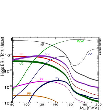
Figure 4: Predictions for SM Higgs boson cross sections at the LHC with $\sqrt{s}=8\,\,\mathrm{TeV}$ (left) YR1 ; YR2 ; YR3 and the decay branching ratios (right) YR1 ; YR2 ; YR3 ; BR . The central lines show the predictions, while the colored bands indicate the theoretical uncertainty.

II.4 Discovery of an SM Higgs-like particle at the LHC

On 4th of July 2012 both ATLAS ATLASdiscovery and CMS CMSdiscovery announced the discovery of a new boson with a mass of $\sim 125.5\,\,\mathrm{GeV}$. This discovery marks a milestone of an effort that has been ongoing for almost half a century and opens up a new era of particle physics. In Fig. 5 one can see the $p_{0}$ values of the search for the SM Higgs boson (with all search channels combined) as presented by ATLAS (left) and CMS (right) in July 2012. the $p_{0}$ value gives the probability that the experimental results observed can be caused by background only, i.e. in this case assuming the absense of a Higgs boson at each given mass. While the $p_{0}$ values are close to $\sim 0.5$ for nearly all hypothetical Higgs boson masses (as would be expected for the absense of a Higgs boson), both experiments show a very low $p_{0}$ value of $p_{0}\sim 10^{-6}$ around $M_{H}\sim 125.5\,\,\mathrm{GeV}$. This corresponds to a discovery of a new particle at the $5\,\sigma$ level by each experiment individually.

Another step in the analysis is a comparison of the measurement of production cross sectinos times branching ratios with the respective SM prediction. Two examples, using LHC data of about $5\,\mbox{fb}^{-1}$ at $7\,\,\mathrm{TeV}$ and about $20\,\mbox{fb}^{-1}$ at $8\,\,\mathrm{TeV}$ are shown in Fig. 6. Here ATLAS ATLAS_5p20ifb (left) and CMS CMS-Higgs-WWW (right) compare their experimental results with the SM prediction in various channels. It can be seen that all channels are, within the theoretical and experimental uncertainties, in agreement with the SM.

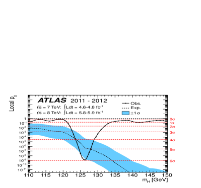
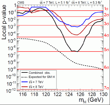
Figure 5: $p_{0}$ values in the SM Higgs boson search (all channels combined) as presented by ATLAS (left) ATLASdiscovery and CMS (right) CMSdiscovery on 4th of July 2012.

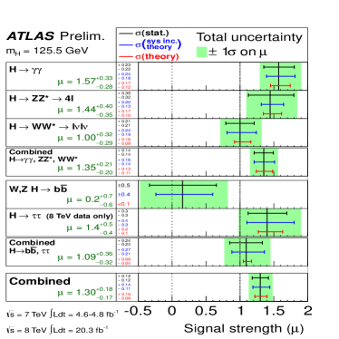
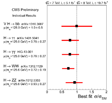
Figure 6: Comparison of the measurement of production cross sectinos times branching ratios with the respective SM prediction from ATLAS ATLAS_5p20ifb (left) and CMS CMS-Higgs-WWW (right).

In this discussion it must be kept in mind that a measurement of the total width and thus of individual couplings is not possible at the LHC (see, e.g., Ref. lhc2tsp and references therein). In the SM, for a fixed value of $M_{H}$, all Higgs couplings to other (SM) particles are specifed. Consequently, it is in general not possible to perform a fit to experimenal data within the SM, where the Higgs couplings are treated as free parameters. Therefore, in order to test the compatibility of the predictions for the SM Higgs boson with the (2012) experimental data, the LHC Higgs Cross Section Working Group proposed several benchmark scenarios for “coupling scale factors” HiggsRecommendation ; YR3 (see Ref. Englert:2014uua for a recent review on Higgs coupling extractions). Effectively, the  predicted SM Higgs cross sections and partial decay widths are dressed with scale factors $\kappa_{i}$ (and $\kappa_{i}=1$ corresponds to the SM). Several assumptions are made for this $\kappa$-framework: there is only one state at $125.5\,\,\mathrm{GeV}$ responsible for the signal, the coupling structure is the same as for the SM Higgs (i.e. it is a ${\cal CP}$-even scalar), and the zero width approximation is assumed to be valid, allowing for a clear separation and simple handling of production and decay of the Higgs particle. The most relevant coupling strength modifiers are $\kappa_{t}$, $\kappa_{b}$, $\kappa_{\tau}$, $\kappa_{W}$, $\kappa_{Z}$, $\kappa_{\gamma}$, $\kappa_{g}$, …

One limitation at the LHC (but not at the ILC) is the fact that the total width cannot be determined experimentally without additional theory assumptions. In the absence of a total width measurement only ratios of $\kappa$’s can be determined from experimental data. An assumption often made is $\kappa_{W,Z}\leq 1$ Duhrssen:2004cv . A recent analysis from CMS using the Higgs decays to $ZZ$ far off-shell yielded an upper limit on the total width about four times larger than the SM width CMS:2014ala . However, here the assumption of the equality of on-shell and off-shell couplings of the Higgs boson plays a crucial role. It was pointed out that this equality is violated in particular in the presense of new physics in the Higgs sector Englert:2014aca .

In the left plot of Fig. 7 we compare the results estimated for the HL-LHC (with $3\mbox{ab}^{-1}$ and an assumed improvement of 50% in the theoretical uncertainties) with the various stages of the ILC under the theory assumption $\kappa_{W,Z}\leq 1$ HiggsCouplings . This most general fit includes $\kappa_{W,Z}$ for the gauge bosons, $\kappa_{u,d,l}$ for up-type quarks, down-type quarks and charged leptons, respectively, as well as $\kappa_{\gamma}$ and $\kappa_{g}$ for the loop-induced couplings of the Higgs to photons and gluons. Also the (possibly invisible) branching ratio of the Higgs boson to new physics (${\rm BR}(H\to{\rm NP})$) is included. One can observe that the HL-LHC and the ILC 250 yield comparable results. However, going to higher ILC energies, yields substantially higher precisions in the fit for the coupling scale factors. In the final stage of the ILC (ILC 1000 LumiUp), precisions at the per-mille level in $\kappa_{W,Z}$ are possible. the $1-2\%$ range is reached for all other $\kappa$’s. The branching ratio to new physics can be restricted to the per-mille level.

Using ILC data the theory assumption $\kappa_{W,Z}\leq 1$ can be dropped, since the “$Z$-recoil method” (see Ref. Baer:2013cma and references therein) allows for a model independent determination of the $HZZ$ coupling. The corresponding results are shown in the right plot of Fig. 7, where the HL-LHC results are combined with the various stages of the ILC. the results from the HL-LHC alone continue to very large values of the $\kappa$’s, since the fit cannot be done without theory assumptions. Including the ILC measurements (where the first line corresponds to the inclusion of only the $\sigma_{ZH}^{\rm total}$ measurement at the ILC) yields a converging fit. In the final ILC stage $\kappa_{W,Z}$ are determined to better than one per-cent, whereas the other coupling scale factors are obtained in the $1-2\%$ range. the branching ratio to new physics is restricted to be smaller than one per-cent.

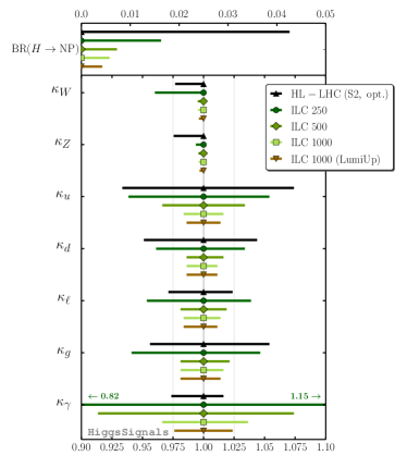
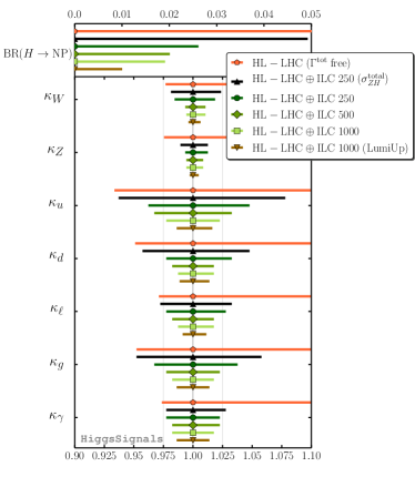
Figure 7: Fit to the coupling scale factors with (left) and without the theory assumptoin of $\kappa_{W,Z}\leq 1$ HiggsCouplings .

III The Higgs in Supersymmetry

III.1 Why SUSY?

Theories based on Supersymmetry (SUSY) mssm are widely considered as the theoretically most appealing extension of the SM. They are consistent with the approximate unification of the gauge coupling constants at the GUT scale and provide a way to cancel the quadratic divergences in the Higgs sector hence stabilizing the huge hierarchy between the GUT and the electroweak (EW) scale. Furthermore, in SUSY theories the breaking of the electroweak symmetry is naturally induced at the EW scale, and the lightest supersymmetric particle can be neutral, weakly interacting and absolutely stable, providing therefore a natural solution for the dark matter problem.

The Minimal Supersymmetric Standard Model (MSSM) constitutes, hence its name, the minimal supersymmetric extension of the SM. the number of SUSY generators is $N=1$, the smallest possible value. In order to keep anomaly cancellation, contrary to the SM a second Higgs doublet is needed glawei . All SM multiplets, including the two Higgs doublets, are extended to supersymmetric multiplets, resulting in scalar partners for quarks and leptons (“squarks” and “sleptons”) and fermionic partners for the SM gauge boson and the Higgs bosons (“gauginos”, “higgsinos” and “gluinos”). So far, the direct search for SUSY particles has not been successful. One can only set lower bounds of ${\cal O}(100\,\,\mathrm{GeV})$ to ${\cal O}(1000\,\,\mathrm{GeV})$ on their masses SUSYMoriond14 ; SUSYMoriond14-QCD .

III.2 The MSSM Higgs sector

An excellent review on this subject is given in Ref. awb2 .

III.2.1 The Higgs boson sector at tree-level

Contrary to the SM, in the MSSM two Higgs doublets are required. The Higgs potential hhg

$$V =m_{1}^{2}|{\cal H}_{1}|^{2}+m_{2}^{2}|{\cal H}_{2}|^{2}-m_{12}^{2}(\epsilon_{ab}{\cal H}_{1}^{a}{\cal H}_{2}^{b}+\mbox{h.c.})$$

$$+\frac{1}{8}(g^{2}+g^{\prime 2})\left[|{\cal H}_{1}|^{2}-|{\cal H}_{2}|^{2}\right]^{2}+\frac{1}{2}g^{2}|{\cal H}_{1}^{{\dagger}}{\cal H}_{2}|^{2}~{},$$ (60)

contains $m_{1},m_{2},m_{12}$ as soft SUSY breaking parameters; $g,g^{\prime}$ are as before the $SU(2)$ and $U(1)$ gauge couplings, and $\epsilon_{12}=-1$.

The doublet fields ${\cal H}_{1}$ and ${\cal H}_{2}$ are decomposed in the following way:

$${\cal H}_{1} =\left(\begin{array}[]{c}{\cal H}_{1}^{0}\\[2.15277pt] {\cal H}_{1}^{-}\end{array}\right)\;=\;\left(\begin{array}[]{c}v_{1}+\frac{1}{\sqrt{2}}(\phi_{1}^{0}-i\chi_{1}^{0})\\[2.15277pt] -\phi_{1}^{-}\end{array}\right)~{},$$ (65)

$${\cal H}_{2} =\left(\begin{array}[]{c}{\cal H}_{2}^{+}\\[2.15277pt] {\cal H}_{2}^{0}\end{array}\right)\;=\;\left(\begin{array}[]{c}\phi_{2}^{+}\\[2.15277pt] v_{2}+\frac{1}{\sqrt{2}}(\phi_{2}^{0}+i\chi_{2}^{0})\end{array}\right)~{}.$$ (70)

${\cal H}_{1}$ gives mass to the down-type fermions, while ${\cal H}_{2}$ gives masses to the up-type fermions. The potential (60) can be described with the help of two independent parameters (besides $g$ and $g^{\prime}$): $\tan\beta=v_{2}/v_{1}$ and $M_{A}^{2}=-m_{12}^{2}(\tan\beta+\cot\beta)$, where $M_{A}$ is the mass of the ${\cal CP}$-odd Higgs boson $A$.

Which values can be expected for $\tan\beta$? One natural choice would be $\tan\beta\approx 1$, i.e. both vevs are about the same. On the other hand, one can argue that $v_{2}$ is responsible for the top quark mass, while $v_{1}$ gives rise to the bottom quark mass. Assuming that their mass differences comes largely from the vevs, while their Yukawa couplings could be about the same. the natural value for $\tan\beta$ would then be $\tan\beta\approx m_{t}/m_{b}$. Consequently, one can expect

$$1\;\raisebox{-3.00003pt}{$\stackrel{{\scriptstyle\displaystyle<}}{{\sim}}$}\;\tan\beta\;\raisebox{-3.00003pt}{$\stackrel{{\scriptstyle\displaystyle<}}{{\sim}}$}\;50~{}.$$ (71)

The diagonalization of the bilinear part of the Higgs potential, i.e. of the Higgs mass matrices, is performed via the orthogonal transformations

$$\left(\begin{array}[]{c}H^{0}\\[2.15277pt] h^{0}\end{array}\right) =\left(\begin{array}[]{cc}\cos\alpha&\sin\alpha\\[2.15277pt] -\sin\alpha&\cos\alpha\end{array}\right)\left(\begin{array}[]{c}\phi_{1}^{0}\\[2.15277pt] \phi_{2}^{0}~{},\end{array}\right)$$ (78)

$$\left(\begin{array}[]{c}G^{0}\\[2.15277pt] A^{0}\end{array}\right) =\left(\begin{array}[]{cc}\cos\beta&\sin\beta\\[2.15277pt] -\sin\beta&\cos\beta\end{array}\right)\left(\begin{array}[]{c}\chi_{1}^{0}\\[2.15277pt] \chi_{2}^{0}\end{array}\right)~{},$$ (85)

$$\left(\begin{array}[]{c}G^{\pm}\\[2.15277pt] H^{\pm}\end{array}\right) =\left(\begin{array}[]{cc}\cos\beta&\sin\beta\\[2.15277pt] -\sin\beta&\cos\beta\end{array}\right)\left(\begin{array}[]{c}\phi_{1}^{\pm}\\[2.15277pt] \phi_{2}^{\pm}\end{array}\right)~{}.$$ (92)

The mixing angle $\alpha$ is determined through

$$\alpha={\rm arctan}\left[\frac{-(M_{A}^{2}+M_{Z}^{2})\sin\beta\cos\beta}{M_{Z}^{2}\cos^{2}\!\beta+M_{A}^{2}\sin^{2}\!\beta-m^{2}_{h,{\rm tree}}}\right]~{},~{}~{}-\frac{\pi}{2}<\alpha<0$$ (93)

with $m_{h,{\rm tree}}$ defined below in Eq. (103).
One gets the following Higgs spectrum:

$$\mbox{2 neutral bosons},\,{\cal CP}=+1 :h,H$$

$$\mbox{1 neutral boson},\,{\cal CP}=-1 :A$$

2 charged bosons $$:H^{+},H^{-}$$

3 unphysical Goldstone bosons $$:G,G^{+},G^{-}.$$ (94)

At tree level the mass matrix of the neutral ${\cal CP}$-even Higgs bosons is given in the $\phi_{1}$-$\phi_{2}$-basis in terms of $M_{Z}$, $M_{A}$, and $\tan\beta$ by

$$M_{\rm Higgs}^{2,{\rm tree}} =\left(\begin{array}[]{cc}m_{\phi_{1}}^{2}&m_{\phi_{1}\phi_{2}}^{2}\\ m_{\phi_{1}\phi_{2}}^{2}&m_{\phi_{2}}^{2}\end{array}\right)=\left(\begin{array}[]{cc}M_{A}^{2}\sin^{2}\!\beta+M_{Z}^{2}\cos^{2}\!\beta&-(M_{A}^{2}+M_{Z}^{2})\sin\beta\cos\beta\\ -(M_{A}^{2}+M_{Z}^{2})\sin\beta\cos\beta&M_{A}^{2}\cos^{2}\!\beta+M_{Z}^{2}\sin^{2}\!\beta\end{array}\right),$$ (99)

which by diagonalization according to Eq. (78) yields the tree-level Higgs boson masses

$$M_{\rm Higgs}^{2,{\rm tree}}\stackrel{{\scriptstyle\alpha}}{{\longrightarrow}}\left(\begin{array}[]{cc}m_{H,{\rm tree}}^{2}&0\\ 0&m_{h,{\rm tree}}^{2}\end{array}\right)$$ (102)

with

$$m_{H,h,{\rm tree}}^{2} =\tfrac{1}{2}\left[M_{A}^{2}+M_{Z}^{2}\pm\sqrt{(M_{A}^{2}+M_{Z}^{2})^{2}-4M_{Z}^{2}M_{A}^{2}\cos^{2}2\beta}\right]~{}.$$ (103)

From this formula the famous tree-level bound

$$m_{h,{\rm tree}}\leq\mbox{min}\{M_{A},M_{Z}\}\cdot|\cos 2\beta|\leq M_{Z}$$ (104)

can be obtained. The charged Higgs boson mass is given by

$$m_{H^{\pm}}^{2}=M_{A}^{2}+M_{W}^{2}~{}.$$ (105)

The masses of the gauge bosons are given in analogy to the SM:

$$M_{W}^{2}=\frac{1}{2}g^{2}(v_{1}^{2}+v_{2}^{2});\qquad M_{Z}^{2}=\frac{1}{2}(g^{2}+g^{\prime 2})(v_{1}^{2}+v_{2}^{2});\qquad M_{\gamma}=0.$$ (106)

The couplings of the Higgs bosons are modified from the corresponding SM couplings already at the tree-level. Some examples are

$$g_{hVV} =\sin(\beta-\alpha)\;g_{HVV}^{\rm SM},\quad V=W^{\pm},Z~{},$$ (107)

$$g_{HVV} =\cos(\beta-\alpha)\;g_{HVV}^{\rm SM}~{},$$ (108)

$$g_{hb\bar{b}},g_{h\tau^{+}\tau^{-}} =-\frac{\sin\alpha}{\cos\beta}\;g_{Hb\bar{b},H\tau^{+}\tau^{-}}^{\rm SM}~{},$$ (109)

$$g_{ht\bar{t}} =\frac{\cos\alpha}{\sin\beta}\;g_{Ht\bar{t}}^{\rm SM}~{},$$ (110)

$$g_{Ab\bar{b}},g_{A\tau^{+}\tau^{-}} =\gamma_{5}\tan\beta\;g_{Hb\bar{b},H\tau^{+}\tau^{-}}^{\rm SM}~{}.$$ (111)

The following can be observed: the couplings of the ${\cal CP}$-even Higgs boson to SM gauge bosons is always suppressed with respect to the SM coupling. However, if $g_{hVV}^{2}$ is close to zero, $g_{HVV}^{2}$ is close to $(g_{HVV}^{\rm SM})^{2}$ and vice versa, i.e. it is not possible to decouple ${\cal CP}$-even Higgs bosons from the SM gauge bosons. The coupling of the $h$ to down-type fermions can be suppressed or enhanced with respect to the SM value, depending on the size of $\sin\alpha/\cos\beta$. Especially for not too large values of $M_{A}$ and large $\tan\beta$ one finds $|\sin\alpha/\cos\beta|\gg 1$, leading to a strong enhancement of this coupling. the same holds, in principle, for the coupling of the $h$ to up-type fermions. However, for large parts of the MSSM parameter space the additional factor is found to be $|\cos\alpha/\sin\beta|<1$. For the ${\cal CP}$-odd Higgs boson an additional factor $\tan\beta$ is found. According to Eq. (71) this can lead to a strongly enhanced coupling of the $A$ boson to bottom quarks or $\tau$ leptons, resulting in new search strategies at the LHC for the ${\cal CP}$-odd Higgs boson, see below.

For $M_{A}\;\raisebox{-3.00003pt}{$\stackrel{{\scriptstyle\displaystyle>}}{{\sim}}$}\;150\,\,\mathrm{GeV}$ the “decoupling limit” is reached. The couplings of the light Higgs boson become SM-like, i.e. the additional factors approach 1. the couplings of the heavy neutral Higgs bosons become similar, $g_{Axx}\approx g_{Hxx}$, and the masses of the heavy neutral and charged Higgs bosons fulfill $M_{A}\approx M_{H}\approx M_{H^{\pm}}$. As a consequence, search strategies for the $A$ boson can also be applied to the $H$ boson, and both are hard to disentangle at hadron colliders (see also Fig. 8 below).

III.2.2 The scalar quark sector

Since the most relevant squarks for the MSSM Higgs boson sector are the $\tilde{t}$ and $\tilde{b}$ particles, here we explicitly list their mass matrices in the basis of the gauge eigenstates $\tilde{t}_{L},\tilde{t}_{R}$ and $\tilde{b}_{L},\tilde{b}_{R}$:

$${\cal M}^{2}_{\tilde{t}} =\left(\begin{array}[]{cc}M_{\tilde{t}_{L}}^{2}+m_{t}^{2}+\cos 2\beta(\tfrac{1}{2}-\frac{2}{3}s_{\mathrm{w}}^{2})M_{Z}^{2}&m_{t}X_{t}\\ m_{t}X_{t}&M_{\tilde{t}_{R}}^{2}+m_{t}^{2}+\frac{2}{3}\cos 2\beta s_{\mathrm{w}}^{2}M_{Z}^{2}\end{array}\right),$$ (114)

$${\cal M}^{2}_{\tilde{b}} =\left(\begin{array}[]{cc}M_{\tilde{b}_{L}}^{2}+m_{b}^{2}+\cos 2\beta(-\tfrac{1}{2}+\frac{1}{3}s_{\mathrm{w}}^{2})M_{Z}^{2}&m_{b}X_{b}\\ m_{b}X_{b}&M_{\tilde{b}_{R}}^{2}+m_{b}^{2}-\frac{1}{3}\cos 2\beta s_{\mathrm{w}}^{2}M_{Z}^{2}\end{array}\right).$$ (117)

$M_{\tilde{t}_{L}}$, $M_{\tilde{t}_{R}}$, $M_{\tilde{b}_{L}}$ and $M_{\tilde{b}_{R}}$ are the (diagonal) soft SUSY-breaking parameters. We furthermore have

$$m_{t}X_{t}=m_{t}(A_{t}-\mu\cot\beta),\quad m_{b}\,X_{b}=m_{b}\,(A_{b}-\mu\tan\beta).$$ (118)

The soft SUSY-breaking parameters $A_{t}$ and $A_{b}$ denote the trilinear Higgs–stop and Higgs–sbottom coupling, and $\mu$ is the Higgs mixing parameter. $SU(2)$ gauge invariance requires the relation

$$M_{\tilde{t}_{L}}=M_{\tilde{b}_{L}}.$$ (119)

Diagonalizing ${\cal M}^{2}_{\tilde{t}}$ and ${\cal M}^{2}_{\tilde{b}}$ with the mixing angles $\theta_{\tilde{t}}$ and $\theta_{\tilde{b}}$, respectively, yields the physical $\tilde{t}$ and $\tilde{b}$ masses: $m_{\tilde{t}_{1}}$, $m_{\tilde{t}_{2}}$, $m_{\tilde{b}_{1}}$ and $m_{\tilde{b}_{2}}$.

III.2.3 Higher-order corrections to Higgs boson masses

A review about this subject can be found in Ref. habilSH . In the Feynman diagrammatic (FD) approach the higher-order corrected ${\cal CP}$-even Higgs boson masses in the MSSM are derived by finding the poles of the $(h,H)$-propagator matrix. the inverse of this matrix is given by

$$\left(\Delta_{\rm Higgs}\right)^{-1}=-i\left(\begin{array}[]{cc}p^{2}-m_{H,{\rm tree}}^{2}+\hat{\Sigma}_{HH}(p^{2})&\hat{\Sigma}_{hH}(p^{2})\\ \hat{\Sigma}_{hH}(p^{2})&p^{2}-m_{h,{\rm tree}}^{2}+\hat{\Sigma}_{hh}(p^{2})\end{array}\right)~{}.$$ (120)

Determining the poles of the matrix $\Delta_{\rm Higgs}$ in Eq. (120) is equivalent to solving the equation

$$\left[p^{2}-m_{h,{\rm tree}}^{2}+\hat{\Sigma}_{hh}(p^{2})\right]\left[p^{2}-m_{H,{\rm tree}}^{2}+\hat{\Sigma}_{HH}(p^{2})\right]-\left[\hat{\Sigma}_{hH}(p^{2})\right]^{2}=0\,.$$ (121)

The very leading one-loop correction to $M_{h}^{2}$ is given by

$$\Delta M_{h}^{2} \sim G_{F}m_{t}^{4}\log\left(\frac{m_{\tilde{t}_{1}}m_{\tilde{t}_{2}}}{m_{t}^{2}}\right)~{},$$ (122)

where $G_{F}$ denotes the Fermi constant. Eq. (122) shows two important aspects: First, the leading loop corrections go with $m_{t}^{4}$, which is a “very large number”. Consequently, the loop corrections can strongly affect $M_{h}$ and push the mass beyond the reach of LEP LEPHiggsSM ; LEPHiggsMSSM and into the mass regime of the newly discovered boson at $\sim 125.5\,\,\mathrm{GeV}$. Second, the scalar fermion masses (in this case the scalar top masses) appear in the log entering the loop corrections (acting as a “cut-off” where the new physics enter). In this way the light Higgs boson mass depends on all other sectors via loop corrections. This dependence is particularly pronounced for the scalar top sector due to the large mass of the top quark and can be used to constrain the masses and mixings in the scalar top sector Mh125 , see below.

The status of the available results for the self-energy contributions to Eq. (120) can be summarized as follows. The complete one-loop result within the MSSM is known ERZ ; mhiggsf1lA ; mhiggsf1lB ; mhiggsf1lC . The by far dominant one-loop contribution is the ${\cal O}(\alpha_{t})$ term due to top and stop loops ($\alpha_{t}\equiv h_{t}^{2}/(4\pi)$, $h_{t}$ being the top-quark Yukawa coupling). the computation of the two-loop corrections has meanwhile reached a stage where all the presumably dominant contributions are available mhiggsletter ; mhiggslong ; mhiggsFD2 ; bse ; mhiggsEP0 ; mhiggsEP1 ; mhiggsEP1b ; mhiggsEP2 ; mhiggsEP3 ; mhiggsEP4 ; mhiggsEP4b ; mhiggsRG1 ; mhiggsRG1a . In particular, the ${\cal O}(\alpha_{t}\alpha_{s})$ contributions to the self-energies – evaluated in the FD as well as in the effective potential (EP) method – as well as the ${\cal O}(\alpha_{t}^{2})$, ${\cal O}(\alpha_{b}\alpha_{s})$, ${\cal O}(\alpha_{t}\alpha_{b})$ and ${\cal O}(\alpha_{b}^{2})$ contributions – evaluated in the EP approach – are known for vanishing external momenta. An evaluation of the momentum dependence at the two-loop level in a pure $\overline{\mathrm{DR}}$ calculation was presented in Ref. mhiggs2lp2 . A (nearly) full two-loop EP calculation, including even the leading three-loop corrections, has also been published mhiggsEP5 . the calculation presented in Ref. mhiggsEP5 is not publicly available as a computer code for Higgs-mass calculations. Subsequently, another leading three-loop calculation of ${\cal O}(\alpha_{t}\alpha_{s}^{2})$, depending on the various SUSY mass hierarchies, has been performed mhiggsFD3l , resulting in the code H3m (which adds the three-loop corrections to the FeynHiggs result). Most recently, a combination of the full one-loop result, supplemented with leading and subleading two-loop corrections evaluated in the Feynman-diagrammatic/effective potential method and a resummation of the leading and subleading logarithmic corrections from the scalar-top sector has been published Mh-logresum in the latest version of the code FeynHiggs feynhiggs ; mhiggslong ; mhiggsAEC ; mhcMSSMlong ; Mh-logresum (also including the leading $p^{2}$ dependend two-loop corrections mhiggs2Lp2 ). While previous to this combination the remaining theoretical uncertainty on the lightest ${\cal CP}$-even Higgs boson mass had been estimated to be about $3\,\,\mathrm{GeV}$ mhiggsAEC ; PomssmRep , the combined result was roughly estimated to yield an uncertainty of about $2\,\,\mathrm{GeV}$ Mh-logresum ; ehowp ; however, more detailed analyses will be necessary to yield a more solid result. Taking the available loop corrections into account, the upper limit of $M_{h}$ is shifted to mhiggsAEC ,

$$M_{h}\leq 135\,\,\mathrm{GeV}~{}$$ (123)

(as obtained with the code FeynHiggs feynhiggs ; mhiggslong ; mhiggsAEC ; mhcMSSMlong ; Mh-logresum ). This limit takes into account the experimental uncertainty for the top quark mass as well as the intrinsic uncertainties from unknown higher-order corrections. Consequently, a Higgs boson with a mass of $\sim 125.5\,\,\mathrm{GeV}$ can naturally be explained by the MSSM.

The charged Higgs boson mass is obtained by solving the equation

$$p^{2}-m_{H^{\pm}}^{2}-\hat{\Sigma}_{H^{-}H^{+}}(p^{2})=0~{}.$$ (124)

For the charged Higgs boson self-energy the full one-loop corrections are known chargedmhiggs ; markusPhD as well as leading two-loop corrections at ${\cal O}(\alpha_{t}\alpha_{s})$ chargedmhiggs2L .

III.3 MSSM Higgs bosons at the LHC

The “decoupling limit” has been discussed above for the tree-level couplings and masses of the MSSM Higgs bosons. This limit also persists taking into account radiative corrections. the corresponding Higgs boson masses are shown in Fig. 8 for $\tan\beta=5$ in the $m_{h}^{\rm max}$ benchmark scenario benchmark2 ; benchmark4 obtained with FeynHiggs. For $M_{A}\;\raisebox{-3.00003pt}{$\stackrel{{\scriptstyle\displaystyle>}}{{\sim}}$}\;180\,\,\mathrm{GeV}$ the lightest Higgs boson mass approaches its upper limit (depending on the SUSY parameters), and the heavy Higgs boson masses are nearly degenerate. Furthermore, also the light Higgs boson couplings including loop corrections approach their SM-value for. Consequently, for $M_{A}\;\raisebox{-3.00003pt}{$\stackrel{{\scriptstyle\displaystyle>}}{{\sim}}$}\;180\,\,\mathrm{GeV}$ an SM-like Higgs boson (below $\sim 135\,\,\mathrm{GeV}$) can naturally be explained by the MSSM. On the other hand, deviations from a SM-like behavior can be described in the MSSM by deviating from the full decoupling limit.

  

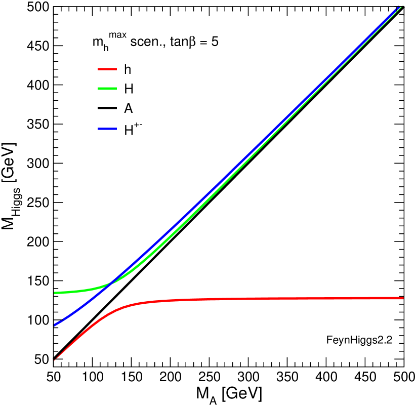
Figure 8: The MSSM Higgs boson masses including higher-order corrections are shown as a function of $M_{A}$ for $\tan\beta=5$ in the $m_{h}^{\rm max}$ benchmark scenario benchmark2 ; benchmark4 (obtained with FeynHiggs feynhiggs ; mhiggslong ; mhiggsAEC ; mhcMSSMlong ; Mh-logresum ).

An example for the various productions cross sections at the LHC is shown in Fig. 9 (for $\sqrt{s}=14\,\,\mathrm{TeV}$). For low masses the light Higgs cross sections are visible, and for $M_{H}\;\raisebox{-3.00003pt}{$\stackrel{{\scriptstyle\displaystyle>}}{{\sim}}$}\;130\,\,\mathrm{GeV}$ the heavy ${\cal CP}$-even Higgs cross section is displayed, while the cross sections for the ${\cal CP}$-odd $A$ boson are given for the whole mass range. As discussed above the $g_{Abb}$ coupling is enhanced by $\tan\beta$ with respect to the corresponding SM value. Consequently, the $b\bar{b}A$ cross section is the largest or second largest cross section for all $M_{A}$, despite the relatively small value of $\tan\beta=5$. For larger $\tan\beta$, see Eq. (71), this cross section can become even more dominant. Furthermore, the coupling of the heavy ${\cal CP}$-even Higgs boson becomes very similar to the one of the $A$ boson, and the two production cross sections, $b\bar{b}A$ and $b\bar{b}H$ are indistinguishable in the plot for $M_{A}>200\,\,\mathrm{GeV}$.

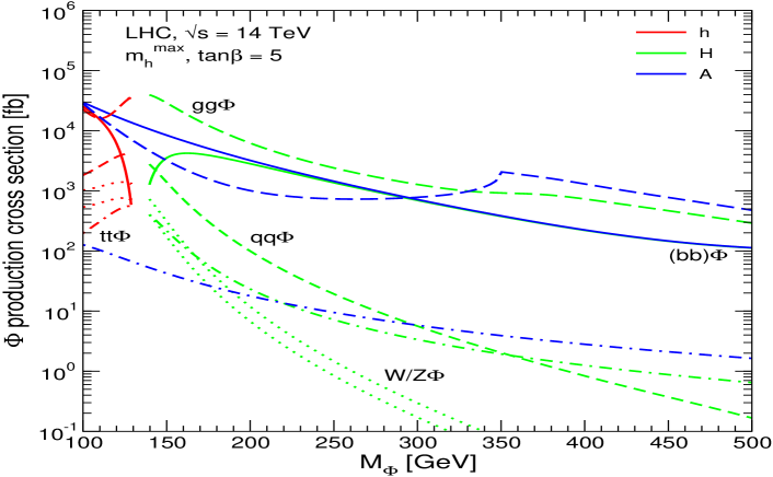
Figure 9: Overview about the various neutral Higgs boson production cross sections at the LHC shown as a function of $M_{A}$ for $\tan\beta=5$ in the $m_{h}^{\rm max}$ scenario (taken from Ref. sigmaH , where the original references can be found).

More precise results in the most important channels, $gg\to\phi$ and $b\bar{b}\to\phi$ ($\phi=h,H,A$) have been obtained by the LHC Higgs Cross Section Working Group lhchxswg , see also Refs. YR1 ; YR2 ; YR3 and references therein. Most recently a new code, SusHi sushi for the $gg\to\phi$ (and $bb\phi$) production mode(s) including the full MSSM one-loop contributions as well as higher-order SM and MSSM corrections has been presented, see Refs. gghMSSM ; gghMSSM2 for more details.

Of particular interest is the “LHC wedge” region, i.e. the region in which only the light ${\cal CP}$-even MSSM Higgs boson, but none of the heavy MSSM Higgs bosons can be detected at the LHC. It appears for $M_{A}\;\raisebox{-3.00003pt}{$\stackrel{{\scriptstyle\displaystyle>}}{{\sim}}$}\;200\,\,\mathrm{GeV}$ at intermediate $\tan\beta$ and widens to larger $\tan\beta$ values for larger $M_{A}$. Consequently, in the “LHC wedge” only a SM-like light Higgs boson can be discovered at the LHC, and part of the LHC wedge (depending on the explicit choice of SUSY parameters) can be in agreement with $M_{h}\sim 125.5\,\,\mathrm{GeV}$. This region, bounded from above by the 95% CL exclusion contours for the heavy neutral MSSM Higgs bosons can be seen in Fig. 10 CMS-HAtautau .

  

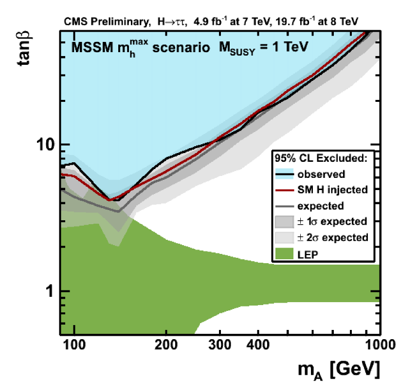
Figure 10: The 95% CL exclusion regions (i.e. the upper bound of the “LHC wedge” region) for the heavy neutral Higgs bosons in the channel $pp\to H/A\to\tau^{+}\tau^{-}(+X)$, obtained by CMS including $\sqrt{s}=7,8\,\,\mathrm{TeV}$ data CMS-HAtautau .

III.4 Agreement of the MSSM Higgs sector with a Higgs at $\sim 125.5\,\,\mathrm{GeV}$

Many investigations have been performed analyzing the agreement of the MSSM with a Higgs boson at $\sim 125.5\,\,\mathrm{GeV}$. In a first step only the mass information can be used to test the model, while in a second step also the rate information of the various Higgs search channels can be taken into account. Here we briefly discuss the results in two of the new benchmark scenarios benchmark4 , devised for the search for heavy MSSM Higgs bosons. In the left plot of Fig. 11 the $m_{h}^{\rm max}$ scenario is shown. the red area is excluded by LHC searches for the heavy MSSM Higgs bosons, the blue area is excluded by LEP Higgs searches, and the light shaded red area is excluded by LHC searches for a SM-like Higgs boson. the bounds have been obtained with HiggsBounds higgsbounds (where an extensive list of original references can be found). the green area yields $M_{h}=125\pm 3\,\,\mathrm{GeV}$, i.e. the region allowed by the experimental data, taking into account the theoretical uncertainty in the $M_{h}$ calculation as discussed above. Since the $m_{h}^{\rm max}$ scenario maximizes the light ${\cal CP}$-even Higgs boson mass it is possible to extract lower (one parameter) limits on $M_{A}$ and $\tan\beta$ from the edges of the green band. By choosing the parameters entering via radiative corrections such that those corrections yield a maximum upward shift to $M_{h}$, the lower bounds on $M_{A}$ and $\tan\beta$ that can be obtained are general in the sense that they (approximately) hold for any values of the other parameters. To address the (small) residual $M_{\rm SUSY}(:=M_{\tilde{t}_{L}}=M_{\tilde{t}_{R}}=M_{\tilde{b}_{R}})$ dependence of the lower bounds on $M_{A}$ and $\tan\beta$, limits have been extracted for the three different values $M_{\rm SUSY}=\{0.5,1,2\}\,\,\mathrm{TeV}$, see Tab. 1 Mh125 . For comparison also the previous limits derived from the LEP Higgs searches LEPHiggsMSSM are shown, i.e. before the incorporation of the Higgs discovery at the LHC. The bounds on $M_{A}$ translate directly into lower limits on $M_{H^{\pm}}$, which are also given in the table. More recent experimental Higgs exclusion bounds shift these limits to even higher values, see the left plot in Fig. 11. Consequently, the experimental result of $M_{h}\sim 125.5\pm 3\,\,\mathrm{GeV}$ requires $M_{H^{\pm}}\;\raisebox{-3.00003pt}{$\stackrel{{\scriptstyle\displaystyle>}}{{\sim}}$}\;m_{t}$ with important consequences for the charged Higgs boson phenomenology.

In the right plot of Fig. 11 we show the $m_{h}^{\rm mod+}$ scenario that differs from the $m_{h}^{\rm max}$ scenario in the choice of $X_{t}$. While in the $m_{h}^{\rm max}$ scenario $X_{t}/M_{\rm SUSY}=+2$ had been chosen to maximize $M_{h}$, in the $m_{h}^{\rm mod+}$ scenario $X_{t}/M_{\rm SUSY}=+1.5$ is used to yield a “good” $M_{h}$ value over the nearly the entire $M_{A}$-$\tan\beta$ plane, which is visible as the extended green region.

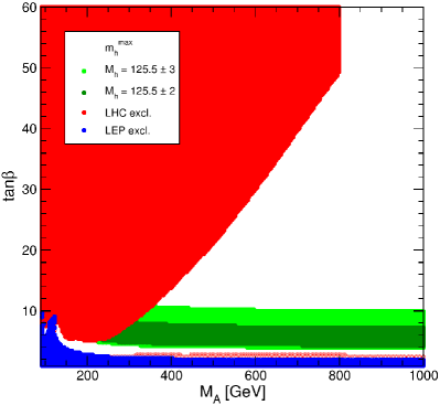
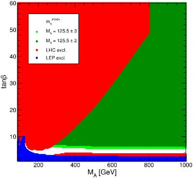
Figure 11: $M_{A}$-$\tan\beta$ plane in the $m_{h}^{\rm max}$ scenario (left) and in the $m_{h}^{\rm mod+}$ scenario (right) benchmark4 . The green shaded area yields $M_{h}\sim 125\pm 3\,\,\mathrm{GeV}$, the red area at high $\tan\beta$ is excluded by LHC heavy MSSM Higgs boson searches, the blue area is excluded by LEP Higgs searches, and the red strip at low $\tan\beta$ is excluded by the LHC SM Higgs searches.

	Limits without $M_{h}\sim 125\,\,\mathrm{GeV}$			Limits with $M_{h}\sim 125\,\,\mathrm{GeV}$
$M_{\rm SUSY}$ (GeV)	$\tan\beta$	$M_{A}$ (GeV)	$M_{H^{\pm}}$ (GeV)	$\tan\beta$	$M_{A}$ (GeV)	$M_{H^{\pm}}$ (GeV)
500	$2.7$	$95$	$123$	$4.5$	$140$	$161$
1000	$2.2$	$95$	$123$	$3.2$	$133$	$155$
2000	$2.0$	$95$	$123$	$2.9$	$130$	$152$

Table 1: Lower limits on the MSSM Higgs sector tree-level parameters $M_{A}$ ($M_{H^{\pm}}$) and $\tan\beta$ obtained with and without the assumed Higgs signal of $M_{h}\sim 125.5\,\,\mathrm{GeV}$. the mass limits have been rounded to $1\,\,\mathrm{GeV}$ Mh125 .

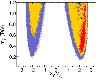
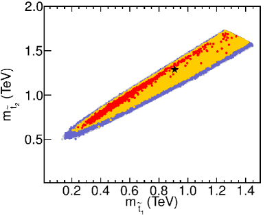
Figure 12: Scalar top mass parameters favored by a $\chi^{2}$ fit to the light Higgs boson mass and the production and decay rates hifi . Red (yellow) points have $\Delta\chi^{2}\leq 2.30(5.99)$. Blue (gray) points were accepted (rejected) by HiggsBounds. Left: $X_{t}/M_{\rm SUSY}$ vs. $m_{\tilde{t}_{1}}$ (with $M_{\rm SUSY}\equiv M_{\tilde{q}_{3}}$); right: $m_{\tilde{t}_{1}}$ vs. $m_{\tilde{t}_{2}}$.

It is also possible to investigate what can be inferred from the assumed Higgs signal about the higher-order corrections in the Higgs sector. In Ref. hifi a scan over seven relevant MSSM parameters has been performed: $M_{A}$, $\tan\beta$, $\mu$, $M_{\rm SUSY}$, $M_{\tilde{l}_{3}}$ (the soft SUSY-breaking parameter for the third generation of scalar leptons), $A_{f}$ (a “universal” trilinear coupling), and $M_{2}$ (the soft SUSY-breaking parameter for gauginos). the measurement of the Higgs boson mass as well as (the then current) results for Higgs boson production and decay rates were taken into account. In Fig. 12 we show the results in the $X_{t}/M_{\rm SUSY}$-$m_{\tilde{t}_{1}}$ plane (left, with $M_{\rm SUSY}\equiv M_{\tilde{q}_{3}}$) and in the $m_{\tilde{t}_{1}}$-$m_{\tilde{t}_{2}}$ plane (right). Blue (gray) points were accepted (rejected) by HiggsBounds. Red (yellow) points have $\Delta\chi^{2}\leq 2.30(5.99)$, thus they constitute the “favored” part of the parameter space. One can see that values of $X_{t}/M_{\rm SUSY}\approx+2$ are preferred. the light scalar top mass can be as low as $\sim 200\,\,\mathrm{GeV}$, while the heavier scalar top mass starts at $\sim 650\,\,\mathrm{GeV}$. A clear correlation between the two masses can be observed (where the scan stopped around $M_{\rm SUSY}\sim 1.5\,\,\mathrm{TeV}$). While no absolute value for any of the stop masses can be obtained, very light masses are in agreement with $M_{h}\sim 125.5$, with interesting prospects for the LHC and the ILC.

Acknowledgments

I thank the organizers for creating a stimulating environment and for their hospitality, in particular when the hotel bar ran out of beer.

References

- (1)
- (2) P. Higgs, Phys. Lett. 12 (1964) 132; Phys. Rev. Lett. 13 (1964) 508; Phys. Rev. 145 (1966) 1156; F. Englert and R. Brout, Phys. Rev. Lett. 13 (1964) 321; G. Guralnik, C. Hagen and T. Kibble, Phys. Rev. Lett. 13 (1964) 585.
- (3) G. Aad et al. [ATLAS Collaboration], Phys. Lett. B 716 (2012) 1 [arXiv:1207.7214 [hep-ex]].
- (4) S. Chatrchyan et al. [CMS Collaboration], Phys. Lett. B 716 (2012) 30 [arXiv:1207.7235 [hep-ex]].
- (5) CDF Collaboration, DØ Collaboration, [arXiv:1207.0449 [hep-ex]].
-
(6)
ATLAS Collaboration, see:
https://twiki.cern.ch/twiki/bin/view/AtlasPublic/HiggsPublicResults . -
(7)
CMS Collaboration, see:
https://twiki.cern.ch/twiki/bin/view/CMSPublic/PhysicsResultsHIG . - (8) S.L. Glashow, Nucl. Phys. B 22 (1961) 579; S. Weinberg, Phys. Rev. Lett. 19 (1967) 19; A. Salam, in: Proceedings of the 8th Nobel Symposium, Editor N. Svartholm, Stockholm, 1968.
- (9) H. Nilles, Phys. Rept. 110 (1984) 1; H. Haber and G. Kane, Phys. Rept. 117 (1985) 75; R. Barbieri, Riv. Nuovo Cim. 11 (1988) 1.
- (10) S. Heinemeyer, O. Stål and G. Weiglein, Phys. Lett. B 710 (2012) 201 [arXiv:1112.3026 [hep-ph]];
- (11) S. Weinberg, Phys. Rev. Lett. 37 (1976) 657; J. Gunion, H. Haber, G. Kane and S. Dawson, The Higgs Hunter’s Guide (Perseus Publishing, Cambridge, MA, 1990), and references therein; G. Branco et al., Phys. Rept. 516 (2012) 1 [arXiv:1106.0034 [hep-ph]]; R. Harlander, M. Muhlleitner, J. Rathsman, M. Spira and O. Stål, arXiv:1312.5571 [hep-ph].
- (12) P. Fayet, Nucl. Phys. B 90 (1975) 104; Phys. Lett. B 64 (1976) 159; Phys. Lett. B 69 (1977) 489; Phys. Lett. B 84 (1979) 416; H.P. Nilles, M. Srednicki and D. Wyler, Phys. Lett. B 120 (1983) 346; J.M. Frere, D.R. Jones and S. Raby, Nucl. Phys. B 222 (1983) 11; J.P. Derendinger and C.A. Savoy, Nucl. Phys. B 237 (1984) 307; J. Ellis, J. Gunion, H. Haber, L. Roszkowski and F. Zwirner, Phys. Rev. D 39 (1989) 844; M. Drees, Int. J. Mod. Phys. A 4 (1989) 3635; U. Ellwanger, C. Hugonie and A. M. Teixeira, Phys. Rept. 496 (2010) 1 [arXiv:0910.1785 [hep-ph]]; M. Maniatis, Int. J. Mod. Phys. A 25 (2010) 3505 [arXiv:0906.0777 [hep-ph]].
- (13) N. Arkani-Hamed, A. Cohen and H. Georgi, Phys. Lett. B 513 (2001) 232 [arXiv:hep-ph/0105239]; N. Arkani-Hamed, A. Cohen, T. Gregoire and J. Wacker, JHEP 0208 (2002) 020 [arXiv:hep-ph/0202089].
- (14) N. Arkani-Hamed, S. Dimopoulos and G. Dvali, Phys. Lett. B 429 (1998) 263 [arXiv:hep-ph/9803315]; Phys. Lett. B 436 (1998) 257 [arXiv:hep-ph/9804398]; I. Antoniadis, Phys. Lett. B 246 (1990) 377; J. Lykken, Phys. Rev. D 54 (1996) 3693 [arXiv:hep-th/9603133]; L. Randall and R. Sundrum, Phys. Rev. Lett. 83 (1999) 3370 [arXiv:hep-ph/9905221].
- (15) G. Weiglein et al. [LHC/ILC Study Group], Phys. Rept. 426 (2006) 47 [arXiv:hep-ph/0410364].
- (16) A. De Roeck et al., Eur. Phys. J. C 66 (2010) 525 [arXiv:0909.3240 [hep-ph]].
-
(17)
LHC2TSP Working Group 1 (EWSB) report, see:
https://indico.cern.ch/
contributionDisplay.py?contribId=131&confId=175067 . - (18) M. Gomez-Bock, M. Mondragon, M. Muhlleitner, M. Spira and P. Zerwas, arXiv:0712.2419 [hep-ph].
- (19) N. Cabibbo, L. Maiani, G. Parisi and R. Petronzio, Nucl. Phys. B 158 (1979) 295; R. Flores and M. Sher, Phys. Rev. D 27 (1983) 1679; M. Lindner, Z. Phys. C 31 (1986) 295; M. Sher, Phys. Rept. 179 (1989) 273; J. Casas, J. Espinosa and M. Quiros, Phys. Lett. 342 (1995) 171. [arXiv:hep-ph/9409458].
- (20) G. Altarelli and G. Isidori, Phys. Lett. B 337 (1994) 141; J. Espinosa and M. Quiros, Phys. Lett. 353 (1995) 257 [arXiv:hep-ph/9504241].
- (21) T. Hambye and K. Riesselmann, Phys. Rev. D 55 (1997) 7255 [arXiv:hep-ph/9610272].
- (22) [The ALEPH, DELPHI, L3 and OPAL Collaborations, the LEP Electroweak Working Group], arXiv:1012.2367 [hep-ex]. see http://lepewwg.web.cern.ch/LEPEWWG/ .
- (23) M. Baak et al., Eur. Phys. J. C 72 (2012) 2205 [arXiv:1209.2716 [hep-ph]].
- (24) See: https://twiki.cern.ch/twiki/bin/view/LHCPhysics/CrossSections .
- (25) S. Dittmaier et al. [LHC Higgs Cross Section Working Group], arXiv:1101.0593 [hep-ph].
- (26) S. Dittmaier et al. [LHC Higgs Cross Section Working Group], arXiv:1201.3084 [hep-ph].
- (27) S. Heinemeyer et al. [LHC Higgs Cross Section Working Group], arXiv:1307.1347 [hep-ph].
- (28) A. Denner, S. Heinemeyer, I. Puljak, D. Rebuzzi and M. Spira, Eur. Phys. J. C 71 (2011) 1753 [arXiv:1107.5909 [hep-ph]].
- (29) ATLAS Collaboration, ATLAS-CONF-2014-009.
- (30) LHC Higgs Cross Section Working Group, A. David et al., arXiv:1209.0040 [hep-ph].
- (31) C. Englert et al., arXiv:1403.7191 [hep-ph].
- (32) J. Baglio et al., JHEP 1304 (2013) 151 [arXiv:1212.5581 [hep-ph]].
- (33) M. Dührssen et al., Phys. Rev. D 70 (2004) 113009 [arXiv:hep-ph/0406323].
- (34) CMS Collaboration, CMS-PAS-HIG-14-002.
- (35) C. Englert and M. Spannowsky, arXiv:1405.0285 [hep-ph].
- (36) P. Bechtle, S. Heinemeyer, O. Stål, T. Stefaniak and G. Weiglein, arXiv:1403.1582 [hep-ph].
- (37) H. Baer et al., arXiv:1306.6352 [hep-ph].
- (38) S. Glashow and S. Weinberg, Phys. Rev. D 15 (1977) 1958.
-
(39)
P. Bargassa,
talk given at “Moriond Electroweak”, March 2014, see:
https://indico.in2p3.fr/materialDisplay.py?contribId=189&sessionId=0 &materialId=slides&confId=9116;
M. Flowerdew, talk given at “Moriond Electroweak”, March 2014, see:
https://indico.in2p3.fr/materialDisplay.py?contribId=169&sessionId=0 &materialId=slides&confId=9116;
C. Petersson, talk given at “Moriond Electroweak”, March 2014, see:
https://indico.in2p3.fr/materialDisplay.py?contribId=155&sessionId=0 &materialId=slides&confId=9116. -
(40)
T. Yamanaka,
talk given at “Moriond QCD”, March 2014, see:
http://moriond.in2p3.fr/QCD/2014/WednesdayMorning/Yamanaka.pdf,
S. Sekmen, talk given at “Moriond QCD”, March 2014, see:
http://moriond.in2p3.fr/QCD/2014/WednesdayMorning/Sekmen.pdf,
D. Olivito, talk given at “Moriond QCD”, March 2014, see:
http://moriond.in2p3.fr/QCD/2014/WednesdayMorning/Olivito.pdf. - (41) A. Djouadi, Phys. Rept. 459 (2008) 1 [arXiv:hep-ph/0503173].
- (42) J. Gunion, H. Haber, G. Kane and S. Dawson, The Higgs Hunter’s Guide, Addison-Wesley, 1990.
- (43) S. Heinemeyer, Int. J. Mod. Phys. A 21 (2006) 2659 [arXiv:hep-ph/0407244].
- (44) LEP Higgs working group, Phys. Lett. B 565 (2003) 61 [arXiv:hep-ex/0306033].
- (45) LEP Higgs working group, Eur. Phys. J. C 47 (2006) 547 [arXiv:hep-ex/0602042].
- (46) J. Ellis, G. Ridolfi and F. Zwirner, Phys. Lett. B 257 (1991) 83; Y. Okada, M. Yamaguchi and T. Yanagida, Prog. Theor. Phys. 85 (1991) 1; H. Haber and R. Hempfling, Phys. Rev. Lett. 66 (1991) 1815.
- (47) A. Brignole, Phys. Lett. B 281 (1992) 284.
- (48) P. Chankowski, S. Pokorski and J. Rosiek, Phys. Lett. B 286 (1992) 307; Nucl. Phys. B 423 (1994) 437 [arXiv:hep-ph/9303309].
- (49) A. Dabelstein, Nucl. Phys. B 456 (1995) 25 [arXiv:hep-ph/9503443]; Z. Phys. C 67 (1995) 495, [arXiv:hep-ph/9409375].
- (50) R. Hempfling and A. Hoang, Phys. Lett. B 331 (1994) 99 [arXiv:hep-ph/9401219].
- (51) S. Heinemeyer, W. Hollik and G. Weiglein, Phys. Rev. D 58 (1998) 091701 [arXiv:hep-ph/9803277]; Phys. Lett. B 440 (1998) 296 [arXiv:hep-ph/9807423].
- (52) S. Heinemeyer, W. Hollik and G. Weiglein, Eur. Phys. Jour. C 9 (1999) 343 [arXiv:hep-ph/9812472].
- (53) R. Zhang, Phys. Lett. B 447 (1999) 89 [arXiv:hep-ph/9808299]; J. Espinosa and R. Zhang, JHEP 0003 (2000) 026 [arXiv:hep-ph/9912236].
- (54) G. Degrassi, P. Slavich and F. Zwirner, Nucl. Phys. B 611 (2001) 403 [arXiv:hep-ph/0105096].
- (55) J. Espinosa and R. Zhang, Nucl. Phys. B 586 (2000) 3 [arXiv:hep-ph/0003246].
- (56) A. Brignole, G. Degrassi, P. Slavich and F. Zwirner, Nucl. Phys. B 631 (2002) 195 [arXiv:hep-ph/0112177].
- (57) A. Brignole, G. Degrassi, P. Slavich and F. Zwirner, Nucl. Phys. B 643 (2002) 79 [arXiv:hep-ph/0206101].
- (58) S. Heinemeyer, W. Hollik, H. Rzehak and G. Weiglein, Eur. Phys. J. C 39 (2005) 465 [arXiv:hep-ph/0411114].
- (59) G. Degrassi, A. Dedes and P. Slavich, Nucl. Phys. B 672 (2003) 144 [arXiv:hep-ph/0305127].
- (60) M. Carena, J. Espinosa, M. Quirós and C. Wagner, Phys. Lett. B 355 (1995) 209 [arXiv:hep-ph/9504316]; M. Carena, M. Quirós and C. Wagner, Nucl. Phys. B 461 (1996) 407 [arXiv:hep-ph/9508343].
- (61) J. Casas, J. Espinosa, M. Quirós and A. Riotto, Nucl. Phys. B 436 (1995) 3, [Erratum-ibid. B 439 (1995) 466] [arXiv:hep-ph/9407389].
- (62) M. Carena, H. Haber, S. Heinemeyer, W. Hollik, C. Wagner, and G. Weiglein, Nucl. Phys. B 580 (2000) 29 [arXiv:hep-ph/0001002].
- (63) S. Martin, Phys. Rev. D 71 (2005) 016012 [arXiv:hep-ph/0405022].
- (64) S. Martin, Phys. Rev. D 65 (2002) 116003 [arXiv:hep-ph/0111209]; Phys. Rev. D 66 (2002) 096001 [arXiv:hep-ph/0206136]; Phys. Rev. D 67 (2003) 095012 [arXiv:hep-ph/0211366]; Phys. Rev. D 68 (2003) 075002 [arXiv:hep-ph/0307101]; Phys. Rev. D 70 (2004) 016005 [arXiv:hep-ph/0312092]; Phys. Rev. D 71 (2005) 116004 [arXiv:hep-ph/0502168]; Phys. Rev. D 75 (2007) 055005 [arXiv:hep-ph/0701051]; S. Martin and D. Robertson, Comput. Phys. Commun. 174 (2006) 133 [arXiv:hep-ph/0501132].
- (65) R. Harlander, P. Kant, L. Mihaila and M. Steinhauser, Phys. Rev. Lett. 100 (2008) 191602 [Phys. Rev. Lett. 101 (2008) 039901] [arXiv:0803.0672 [hep-ph]]; JHEP 1008 (2010) 104 [arXiv:1005.5709 [hep-ph]].
- (66) T. Hahn, S. Heinemeyer, W. Hollik, H. Rzehak and G. Weiglein, Phys. Rev. Lett. 112 (2014) 141801 [arXiv:1312.4937 [hep-ph]].
- (67) G. Degrassi, S. Heinemeyer, W. Hollik, P. Slavich and G. Weiglein, Eur. Phys. J. C 28 (2003) 133 [arXiv:hep-ph/0212020].
- (68) S. Heinemeyer, W. Hollik and G. Weiglein, Comput. Phys. Commun. 124 (2000) 76 [arXiv:hep-ph/9812320]; T. Hahn, S. Heinemeyer, W. Hollik, H. Rzehak and G. Weiglein, Comput. Phys. Commun. 180 (2009) 1426, see: http://www.feynhiggs.de .
- (69) M. Frank, T. Hahn, S. Heinemeyer, W. Hollik, H. Rzehak and G. Weiglein, JHEP 0702 (2007) 047 [arXiv:hep-ph/0611326].
- (70) S. Borowka, T. Hahn, S. Heinemeyer, G. Heinrich and W. Hollik, arXiv:1404.7074 [hep-ph].
- (71) S. Heinemeyer, W. Hollik and G. Weiglein, Phys. Rept. 425 (2006) 265 [arXiv:hep-ph/0412214].
- (72) O. Buchmueller et al., Eur. Phys. J. C 74 (2014) 2809 [arXiv:1312.5233 [hep-ph]].
- (73) M. Diaz and H. Haber, Phys. Rev. D 45 (1992) 4246.
- (74) M. Frank, PhD thesis, university of Karlsruhe, 2002.
- (75) M. Frank et al., Phys. Rev. D 88 (2013) 5, 055013 [arXiv:1306.1156 [hep-ph]].
- (76) M. Carena, S. Heinemeyer, C. Wagner and G. Weiglein, Eur. Phys. J. C 26 (2003) 601 [arXiv:hep-ph/0202167].
- (77) M. Carena, S. Heinemeyer, O. Stål, C. Wagner and G. Weiglein, Eur. Phys. J. C 73 (2013) 2552 [arXiv:1302.7033 [hep-ph]].
- (78) T. Hahn, S. Heinemeyer, F. Maltoni, G. Weiglein and S. Willenbrock, arXiv:hep-ph/0607308.
- (79) R. Harlander, S. Liebler and H. Mantler, Comput. Phys. Commun. 184 (2013) 1605 [arXiv:1212.3249 [hep-ph]].
- (80) R. Harlander and M. Steinhauser, JHEP 0409 (2004) 066 [arXiv:hep-ph/0409010]; C. Anastasiou, S. Beerli, S. Bucherer, A. Daleo and Z. Kunszt, JHEP 0701 (2007) 082 [arXiv:hep-ph/0611236]; U. Aglietti, R. Bonciani, G. Degrassi and A. Vicini, JHEP 0701 (2007) 021 [arXiv:hep-ph/0611266]; M. Muhlleitner and M. Spira, Nucl. Phys. B 790 (2008) 1 [arXiv:hep-ph/0612254]; G. Degrassi and P. Slavich, Nucl. Phys. B 805 (2008) 267 [arXiv:0806.1495 [hep-ph]]; G. Degrassi, S. Di Vita and P. Slavich, JHEP 1108 (2011) 128 [arXiv:1107.0914 [hep-ph]]; Eur. Phys. J. C 72 (2012) 2032 [arXiv:1204.1016 [hep-ph]]; A. Pak, M. Rogal and M. Steinhauser, JHEP 1002 (2010) 025 [arXiv:0911.4662 [hep-ph]]; R. Harlander, H. Mantler, S. Marzani and K. Ozeren, Eur. Phys. J. C 66 (2010) 359 [arXiv:0912.2104 [hep-ph]]; R. Harlander, F. Hofmann and H. Mantler, JHEP 1102 (2011) 055 [arXiv:1012.3361 [hep-ph]]; A. Pak, M. Steinhauser and N. Zerf, JHEP 1209 (2012) 118 [arXiv:1208.1588 [hep-ph]]; Eur. Phys. J. D 71 (2011) 1602 [Erratum-ibid. C 72 (2012) 2182] [arXiv:1012.0639 [hep-ph]].
- (81) E. Bagnaschi et al., arXiv:1404.0327 [hep-ph].
- (82) CMS Collaboration, CMS-PAS-HIG-13-021.
- (83) P. Bechtle, O. Brein, S. Heinemeyer, G. Weiglein and K. E. Williams, Comput. Phys. Commun. 181 (2010) 138 [arXiv:0811.4169 [hep-ph]]; Comput. Phys. Commun. 182 (2011) 2605 [arXiv:1102.1898 [hep-ph]]; P. Bechtle, O. Brein, S. Heinemeyer, O. Stål, T. Stefaniak, G. Weiglein and K. Williams, Eur. Phys. J. C 74 (2014) 2693 [arXiv:1311.0055 [hep-ph]].
- (84) P. Bechtle, S. Heinemeyer, O. Stål, T. Stefaniak, G. Weiglein and L. Zeune, Eur. Phys. J. C 73 (2013) 2354 [arXiv:1211.1955 [hep-ph]].