One possible solution of peculiar type Ia supernovae explosions caused by a charged white dwarf

Abstract

Recent astrophysics observation reveals the existence of some super luminous type Ia supernovae. One natural explanation of such a peculiar phenomenon is to require the progenitor of such a supernova to be a highly super-Chandrasekhar mass white dwarf. Along this line, in this paper, we propose a possible mechanism to explain this phenomenon based on a charged white dwarf. In particular, by choosing suitable new variables and a representative charge distribution, an analytic solution is obtained. The stability issue is also discussed, remarkably, it turns out that the charged white dwarf configuration can be dynamically stable. Moreover, we investigate the general relativistic effects and it is shown that the general relativistic effects can be negligible when the mass of the charged white dwarf is below about $3M_{\odot}$.

I Introduction

It is generally believed that type Ia supernovae can be regarded as standard candles in the measurement of cosmological distance. However, some peculiar type Ia supernovae, e.g., SN2003fg, SN2006gz, SN2007if and SN2009dc Howell06 ; Scalzo10 have been observed recently. Contrast with the standard Ia supernovae, these objects have exceptionally higher luminosity but with lower kinetic energies. In order to understand these phenomenon, some authors assume that the progenitor of such supernova to be a highly super-Chandrasekhar mass white dwarf. If the masses of progenitors of above supernovae lie in the range $2.1M_{\odot}\sim 2.8M_{\odot}$ Howell06 ; Scalzo10 ; Hicken07 ; Yamanaka09 ; Silverman11 ; Taubenberger11 , here $M_{\odot}$ being the mass of sun, this hypothesis can explain experiment data naturally. Hence along this line, the authors of references Mukhopadhyay12 ; Das12 ; Das13 propose a mechanism to generate super-Chandrasekhar mass white dwarf by assuming the existence of a super strong uniform magnetic fields inside the white dwarf. However, it becomes a debate issue, although this picture can uplift the mass of white dwarf significantly, it questioned by several authors with its stability issues Zuo14 , including neutronization induced by inverse beta decay CFD13 , dynamical instability as demonstrated by literature Ruffini13 . Reply of those criticism can be found inDM14a ; DM14b . Now a natural question is that does it exist any other possibility to form a highly super-Chandrasekhar white dwarf? Can we find a stable configuration significant violating the Chandrasekhar mass limit? If it exists, then what is the ultimate mass limit of a white dwarf? Here we plan to address all the above issues by exploiting the electric field effects inside the compact star.

In fact, there is a long history of studying the charge effects in compacted objects, especially in neutron stars and quark stars Bekenstein71 ; Dionysiou82 ; Lemos03 ; Ghezzi05 ; Lun07 ; Usov09 . One important conclusion is that a net charge distribution can support a higher maximum mass of compact star significantly. While in white dwarf, there are also several authors concern the charge effects, for instance in reference Olson76 , a two components charge fluid model of white dwarf has been proposed. However, in Olson76 they still assume that the net charge of white dwarf is very tiny as people generally believed. Along this line, here we propose a new mechanism: assuming existence of strongly charged white dwarf to support the super-Chandrasekhar white dwarf. Although this assumption has not yet confirmed by observation, it still can serve as a useful toy model, especially in the theoretical discussion. In this new picture, we believe that most of the white dwarf is nearly neutral and the Chandrasekhar mass limit still remains valid for most of the white dwarf, just as the astro observations indicated. However, there may exist some white dwarfs, if enough net charge distributes in the star, as the force between the charged particles is repulsive and thus equivalently can stiffen the equation of state of the white dwarf matters, then the maximum mass of the charged white dwarf should be significantly enlarged. Therefore, this in turn can provide a natural mechanism to explain the peculiar type Ia supernova explosion as mentioned in the beginning.

Contrast with the magnetic field effect, one of the most striking feature of charged white dwarf is its dynamical stability. The major difference between electric field and magnetic field is that there exists an exactly spherical symmetry electrostatic field, while a spherical symmetric magnetostatic field is not even existed. Thus unlike the magnetized white dwarf, the structure of charged white dwarf will not be deformed by the non-spherical symmetric field.

This paper is organized as follows: After a short introduction, we present the basic structure formulation of the charged white dwarf and the corresponding numerical results in Sec. II, where two subsections are included. The exact solution of the charged white dwarf is obtained in subsection A, and the numerical results are shown in subsection B. The stability issue of the charged white dwarf is examined in Sec. III, and the general relativistic effects on the charged white dwarf are shown in Sec. IV. Conclusions and outlooks are given in the last section.

II Hydrostatic Equilibrium Equation of Charged White Dwarf

For a static and spherical symmetric charged white dwarf, the outward force induced by the degenerate electron gas and the repulsive electrostatic force caused by the net charge are balanced by the inward gravitational force. In the Newtonian framework, the hydrostatic equilibrium equation can be written as

$$\frac{dp}{dr}=-\frac{Gm\rho}{r^{2}}+\frac{qdq}{16\pi^{2}\varepsilon_{0}r^{4}dr},$$ (1)

where $p$ and $\rho$ are the pressure and the mass density, respectively; the net charges $q$ inside the radius $r$ can be calculated by

$$q(r)=\int_{0}^{r}4\pi\rho_{q}r^{2}dr,$$ (2)

in which $\rho_{q}$ is the charge density; and the stellar mass $m$ inside the radius $r$ is related with the matter density through

$$\frac{dm}{dr}=4\pi r^{2}\rho.$$ (3)

In addition, we use the capital letters $M$, $Q$ denote the total mass and total charge of a charged white dwarf. In order to simplify the discussion, we assume the charge density of white dwarf proportional to its matter density, ie

$$\rho_{q}=\alpha\times\frac{e}{m_{{}_{p}}}\times\rho,$$ (4)

where $\alpha$ is a dimensionless constant, $e$ and $m_{{}_{p}}$ are the charge and mass of a proton, respectively. Note that this kind of charge distribution is also adopted by many other authorsLemos03 ; Usov09 . Moreover, since our electric field can be regarded as a particular case of anisotropic matterHB13a ; HB13b , therefore the following subsection A can be viewed as a direct application of the general formalism of polytropic Newtonian star with anisotropic pressure developed by Herrera and Barreto HB13a .

II.1 exact solution for polytropic equation of state

Combining Eqs. (1)-(3), through a careful and complicated calculation, we obtain an exact solution by choosing the equation of state with a form of polytropic type $p=\kappa\rho^{\gamma}=\kappa\rho^{1+\frac{1}{n}}$, where $n$ is an integer. By using the charge distribution of Eq. (4), the equilibrium equation (1) can be reduced to

$$\frac{dp}{dr} = -\frac{Gm\rho}{r^{2}}\left[1-\frac{\alpha^{2}e^{2}}{Gm_{p}^{2}4\pi\varepsilon_{0}}\right]$$ (5)

$$= -\frac{Gm\rho}{r^{2}}\left[1-\alpha^{2}\beta\right],$$

where $\beta=\frac{e^{2}}{Gm_{p}^{2}4\pi\varepsilon_{0}}=1.24\times 10^{36}$ is also a dimensionless constant. Combining this result with Eq.(3), we get

$$\frac{1}{r^{2}}\frac{d}{dr}\left(\frac{r^{2}dp}{\rho dr}\right)=-4\pi G\rho\left[1-\alpha^{2}\beta\right].$$ (6)

Now we introduce two new variables defined by

$$\rho=\rho_{c}\theta^{n},\quad\quad\xi=\frac{r}{a},$$ (7)

where $\rho_{c}$ is the central density of the white dwarf and $a$ is a constant defined by

$$a=\left[\frac{(n+1)\kappa\rho_{c}^{\frac{1}{n}-1}}{4\pi G\left(1-\alpha^{2}\beta\right)}\right]^{\frac{1}{2}}.$$ (8)

By using these new defined variables and the polytropic form of equation of state, Eq.(1) is reduced to the standard form of Lane-Emden equationWeinberg72

$$\frac{d}{d\xi}\left(\xi^{2}\frac{d\theta}{d\xi}\right)+\theta^{n}\xi^{2}=0.$$ (9)

By employing the standard boundary conditions

$$\theta(\xi=0)=1,\quad\quad\frac{d\theta}{d\xi}\Big{|}_{\xi=0}=0,$$ (10)

Eq.(9) can be solved analytically. The radius of white dwarf relates to a finite value of $\xi=\xi_{1}$ with $R=a\xi_{1}$, where $\xi_{1}$ is the first zero point of $\theta$ function. Meanwhile, the mass of white dwarf can be obtained by combining Eqs. (3),(7),(9)

$$M = \int_{0}^{R}4\pi r^{2}\rho(r)dr$$ (11)

$$= 4\pi a^{3}\rho_{c}\int_{0}^{\xi_{1}}\xi^{2}\theta^{n}d\xi$$

$$= 4\pi a^{3}\rho_{c}\xi_{1}^{2}{\left|{\theta^{\prime}(\xi_{1})}\right|}.$$

It is worth noting that when the index $\gamma=\frac{4}{3}$ (or equivalently $n=3$), the mass of charged white dwarf becomes independent with $\rho_{c}$, and thus corresponds with the maximal mass of charged white dwarf. By comparing these results with the uncharged white dwarf, it is easy to see that the difference is only reflected by the definition of $a$, i.e. we have

$$R=\frac{R_{Ch}}{\left(1-\alpha^{2}\beta\right)^{\frac{1}{2}}},\quad\quad M=\frac{M_{Ch}}{\left(1-\alpha^{2}\beta\right)^{\frac{3}{2}}}$$ (12)

where $R_{Ch}$ and $M_{Ch}$ are the Chandrasekhar radius and Chandrasekhar mass limit for uncharged white dwarf, respectively. Finally, it is worth noting that when $\alpha=0$ the Chandrasekhar mass limit of uncharged white dwarf will be recovered perfectly.

II.2 numerical solution for general equation of state

It is generally believed that the equation of state of white dwarfs can be simply described by the equation of state of the free electron gas

$$k_{{}_{F}}=\hbar(\frac{3\pi^{2}\rho}{m_{p}\mu})^{1/3},$$ (13)

$$p=\frac{8\pi c}{3(2\pi\hbar)^{3}}\int_{0}^{k_{F}}\frac{k^{2}}{(k^{2}+m_{e}^{2}c^{2})^{1/2}}k^{2}dk$$ (14)

where $k$ represents the momentum of electrons, $k_{F}$ is the maximum momentum determined by mass density, $\mu$ is the ratio of nucleon numbers to electron numbers. It is easy to see that even in this simple case, the equation of state still can not be attributed to polytropic type, and thus become difficult to be solved analytically. In view of these facts, the equations (1)-(3) should be treated by numerical calculation.

Combining the above equation of state with the Newtonian equilibrium equations (1)-(3) and the boundary conditions: $m=0$ at $r=0$ and $p=0$ at $r=R$, we can obtain the mass-radius relation for charged white dwarf numerically. the numerical results for the charged and uncharged white dwarf are presented in Fig. 1. From this figure it is shown that at a fixed radius, a higher charge density corresponds with a higher stellar mass. When the $\alpha$ takes a range from $4.0\times 10^{-19}$ to $5.0\times 10^{-19}$, the corresponding maximum mass of charged white dwarf varies from $2.0M_{\odot}$ to $2.5M_{\odot}$ continuously. Hence this picture can naturally explain the recent observational data.

In order to show the structures and properties of the charged white dwarf intuitively, and also compare them to that of the uncharged white dwarf, the numerical results are presented in the Figs. (2)-(5). In Fig. 2, the $Q$ (total charge)-$M$ (stellar mass) relations and the $Q$-$R$ (stellar radius) relations are plotted. And in order to see the charge influence on a single white dwarf more clearly, we plot the pressure and mass distribution in Fig. 3 for $\rho_{c}=1.9\times 10^{13}kg/m^{3}$ and $\alpha=5.0\times 10^{-19}$, where the distributions of corresponding uncharged white dwarf are also plotted. Moreover, in Fig. 4 we show the charge density and the total charge as functions of radius $r$ at the same $\rho_{c}$ and $\alpha$ as used in Fig. 3. In the end, the $M$-$\alpha$, $M$-$Q$ and $M$-$R$ relations at $\rho_{c}=1.9\times 10^{13}kg/m^{3}$ are shown in Fig. 5. It is interesting to note that when $\alpha$ is smaller than $1\times 10^{-20}$, the charge effects on the mass-radius relation of white dwarf can be negligible. However, when we further increase $\alpha$ to reach the order of $10^{-19}$, the maximal mass of corresponding charged white dwarf will become sensitive to the value of $\alpha$, and will grow up very rapidly as $\alpha$ increases.

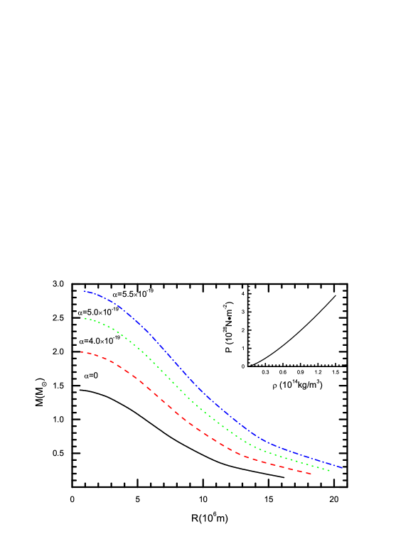
Figure 1: The mass-radius relations of the charged white dwarf, where the different lines represent the different value of $\alpha$ and the central density ranges from $5\times 10^{8}kg/m^{3}$ to $1.37\times 10^{14}kg/m^{3}$. The inset shows the equation of state of free electron gas.

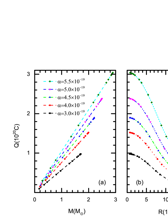
Figure 2: The Q-M relations (a) and the Q-R relations (b) for different values of $\alpha$.

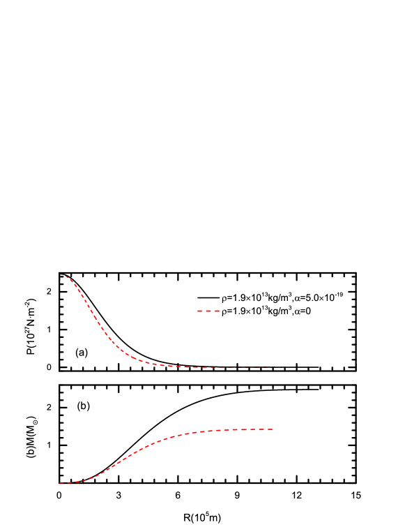
Figure 3: The pressure distribution (a) and mass distribution (b) for the charged (solid lines) and uncharged (dashed lines) white dwarf at a fixed central density $\rho_{c}=1.9\times 10^{13}kg/m^{3}$.

Figure 4: The charge density (a) and the total charge (b) as functions of radius $r$, where $\rho_{c}=1.9\times 10^{13}kg/m^{3}$, and $\alpha=5.0\times 10^{-19}$.

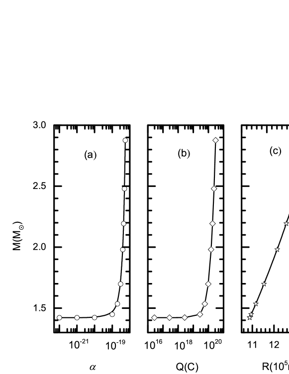
Figure 5: The M-$\alpha$, M-Q and M-R relations, where $\rho_{c}=1.9\times 10^{13}kg/m^{3}$.

III The Stability of The Charged White Dwarf

Since we have already known that a super strong magnetic field in white dwarf will cause the whole system dynamical instabilityZuo14 ; CFD13 ; Ruffini13 , hence when one introduce a strong electric field in white dwarf, it is crucial to investigate the same stability issues. Based on the results in Sec. II, it is shown that the mass of charged white dwarf reaches its maximal value with a central density blow than the neutralizing densityCFD13 , thus our model can avoid the instability caused by neutralization.

On the other hand, in a seminal paperCF53 , Chandrasekhar and Fermi generalize the Viral theorem including the magnetic field and it in turn sets a constraint on the value of magnetic field. Based on this famous result, another kind of instability of white dwarf with a super strong magnetic field is introduced by Ruffni et.al.Ruffini13 . Does this kind of instability also existed in white dwarf with super strong electric field? To answer this question, we use the similar strategy of reference CF53 , that is, to generalize the Virial theorem including the electric field:

$$3\Pi+W_{{}_{E}}+W_{{}_{G}}=0.$$ (15)

For a polytropic equation of state $P=K\rho^{\gamma}$, we can get $\Pi=(\gamma-1)U$, where $U$ is the internal energy. In order to proof this theorem, we start from the usual assumptions of electrohydrodynamics Castellanos98 ; Zhakin12 . The equations of motion governing an inviscid fluid can be written in the form Zhakin12

$$\rho\frac{du_{i}}{dt}=-\frac{\partial}{\partial x_{i}}(p+\frac{\varepsilon_{r}\varepsilon_{0}|E|^{2}}{2})+\rho\frac{\partial\Omega}{\partial x_{i}}+\varepsilon_{r}\varepsilon_{0}\frac{\partial}{\partial x_{j}}\left(E_{i}E_{j}\right)$$ (16)

where $\rho$ and $p$ denote the density and pressure of the charged fuild respectively, $\varepsilon_{r}$ is relative permittivity, $\Omega$ is the gravitational potential, and $E$ is the intensity of the electric field. Multiply Eq. (16) by $x_{i}$ and integrate over the volume of the configuration, then the left-hand side of the equation reads

$$\int\int\int\rho x_{i}\frac{du_{i}}{dt}dx_{1}dx_{2}dx_{3} =\int_{0}^{M}x_{i}\frac{d^{2}x_{i}}{dt^{2}}dm$$ (17)

$$=\int_{0}^{M}\left[\frac{d}{dt}(x_{i}\frac{dx_{i}}{dt})-(\frac{dx_{i}}{dt})^{2}\right]dm$$

$$=\int_{0}^{M}\frac{d}{dt}(\frac{1}{2}\frac{dx_{i}^{2}}{dt})dm-\int_{0}^{M}(\frac{dx_{i}}{dt})^{2}dm$$

$$=\frac{1}{2}\frac{d^{2}}{dt^{2}}\int_{0}^{M}r^{2}dm-\int_{0}^{M}|u|^{2}dm$$

where $dm=\rho dx_{1}dx_{2}dx_{3}$ and $M$ is the total mass of the configuration. Letting

$$I=\int_{0}^{M}r^{2}dm\qquad\textrm{and}\qquad T=\frac{1}{2}\int|u|^{2}dm$$ (18)

represent the moment of inertia and the kinetic energy of mass motion, respectively, we can rewrite the Eq. (16) as

$$\frac{1}{2}\frac{d^{2}I}{dt^{2}}-2T=-\int\int\int x_{i}\frac{\partial}{\partial x_{i}}(p+\varepsilon_{r}\varepsilon_{0}\frac{|E|^{2}}{2})dx_{1}dx_{2}dx_{3}+\varepsilon_{r}\varepsilon_{0}\int\int\int x_{i}\frac{\partial}{\partial x_{j}}\left(E_{i}E_{j}\right)dx_{1}dx_{2}dx_{3}+\int_{0}^{M}x_{i}\frac{\partial\Omega}{\partial x_{i}}dm.$$ (19)

The last term of the right-hand side of this equation represents the gravitational potential energy of the configuration:

$$W_{G} = \int_{0}^{M}x_{i}\frac{\partial\Omega}{\partial x_{i}}dm=-\int_{0}^{M}\frac{Gm(r)}{r}dm(r)$$ (20)

$$= -\frac{3(\gamma-1)}{5\gamma-6}\frac{GM^{2}}{R},$$

where the fact that the charged white dwarf configuration being spherical symmetric is employed. The remaining two terms of equation (19) can also be reduced through integration by parts

$$-\int\int\int x_{i}\frac{\partial}{\partial x_{i}}(p+\varepsilon_{r}\varepsilon_{0}\frac{|E|^{2}}{2})dx_{1}dx_{2}dx_{3} =-\int\int\int\left[\frac{\partial}{\partial x_{i}}\left(x_{i}(p+\varepsilon_{r}\varepsilon_{0}\frac{|E|^{2}}{2})\right)-\left(\frac{\partial x_{i}}{\partial x_{i}}\right)(p+\varepsilon_{r}\varepsilon_{0}\frac{|E|^{2}}{2})\right]dx_{1}dx_{2}dx_{3}$$ (21)

$$=-\int(p+\varepsilon_{r}\varepsilon_{0}\frac{|E|^{2}}{2})\textbf{r}\cdot d\textbf{s}+3\int\int\int(p+\varepsilon_{r}\varepsilon_{0}\frac{|E|^{2}}{2})dx_{1}dx_{2}dx_{3}.$$

The surface integral over $d\textbf{s}$ vanishes as the pressure (including the electric pressure $\varepsilon_{r}\varepsilon_{0}\frac{|E|^{2}}{2}$) must vanish on the boundary of the configuration; and it is easy to see that the volume integral over $p$ and $\varepsilon_{r}\varepsilon_{0}\frac{|E|^{2}}{2}$ give the internal energy ($U$) and the electric energy ($W_{E}$) of the configuration. Thus we have

$$-\int\int\int x_{i}\frac{\partial}{\partial x_{i}}(p+\varepsilon_{r}\varepsilon_{0}\frac{|E|^{2}}{2})dx_{1}dx_{2}dx_{3}=3(\gamma-1)U+3W_{E},$$ (22)

where the relation $p=(\gamma-1)\epsilon$ Weinberg72 is used, and as $\epsilon=\rho-m_{N}n$ is the density of internal energy, here $m_{N}=1.66\times 10^{-27}kg$ being the rest mass per nucleon. Thus the volume integral of $\epsilon$ gives the total heat energy $U$. In the same manner, the second volume integral in equation (19) gives

$$\varepsilon_{r}\varepsilon_{0}\int\int\int x_{i}\frac{\partial}{\partial x_{j}}\left(E_{i}E_{j}\right)dx_{1}dx_{2}dx_{3}=-2W_{E}.$$ (23)

Now, combining equations (19)(22)(23), we have

$$\frac{1}{2}\frac{d^{2}I}{dt^{2}}=2T+3(\gamma-1)U+W_{E}+W_{G}$$ (24)

This is just the generalized version of the Virial theorem including electric field, it differs from the usual one only in the appearance of $W_{E}+W_{G}$ in place of $W_{G}$.

By applying this generalized Virial theorem to a charged non-rotating equilibrium star, then above equation reduce to

$$3(\gamma-1)U+W_{E}+W_{G}=0$$ (25)

This is nothing but Eq.(15) we want to prove. With the help of the expression of charge density described by Eq. (4), the electric energy $W_{E}$ appeared in the above equation can also be integrated exactly:

$$W_{{}_{E}} = \int_{0}^{R}\frac{1}{2}\varepsilon_{0}(\frac{q(r)}{4\pi\varepsilon_{0}r^{2}})^{2}4\pi r^{2}dr=\int_{0}^{R}\frac{q^{2}(r)}{8\pi\varepsilon_{0}r^{2}}dr$$ (26)

$$= \frac{\alpha^{2}e^{2}}{m_{p}^{2}}\int_{0}^{R}\frac{m^{2}(r)}{8\pi\varepsilon_{0}r^{2}}dr$$

$$= \frac{\alpha^{2}\beta}{2}\int_{0}^{R}\frac{Gm^{2}(r)}{r^{2}}dr$$

$$= \frac{\alpha^{2}\beta}{2}\frac{\gamma}{(5\gamma-6)}\frac{GM^{2}}{R}$$

Here, for simplicity and without loss any generality, we assume relative permittivity $\varepsilon_{r}=1$. If $\varepsilon_{r}>1$, the electric field energy will be suppressed by a factor $\varepsilon_{r}$ and thus such a $\varepsilon_{r}$ will make the whole system more stable. Now we define the total energy of the configuration by

$$W_{\textrm{total}}=U+W_{{}_{E}}+W_{G},$$ (27)

as the gravitational potential energy of the configuration $W_{G}$ is negative, in order to form a bounded star configuration, the value of other positive energy such as electric energy and heat energy, should not be larger than the value of the negative gravitational potential energy. Hence similar to the results of reference CF53 , a necessary condition for the dynamical stability of a charged white dwarf equilibrium configuration should be $W_{total}<0$. By eliminating $U$ between Eqs. (15) and (27), one can obtain

$$W_{total} = -\frac{3\gamma-4}{3(\gamma-1)}(|W_{{}_{G}}|-W_{{}_{E}}).$$ (28)

According to above equation, one can find that if the electric energy is larger than the gravitational potential energy, even for $\gamma>\frac{4}{3}$( the condition of dynamical stability in the absence of electric fieldWeinberg72 ), the whole system can also be dynamical instability. However, we can see that this is not the case, as this will require

$$1<\frac{W_{E}}{|W_{{}_{G}}|}=\frac{\frac{\alpha^{2}\beta}{2}\gamma}{3(\gamma-1)},$$ (29)

combining this condition with $\gamma>\frac{4}{3}$ led to $\alpha^{2}\beta>\frac{3}{2}$, however, this is inconsistence with Eq.(12) which states $\alpha^{2}\beta<1$. Hence, in conclusion, for $\gamma>\frac{4}{3}$, the charged white dwarf is dynamically stable. In addition, it is easy to see that when $\alpha=0$ (i.e. uncharged white dwarf), our conclusion is nicely coincide with the well known result in reference Weinberg72 .

IV General Relativity Effects of The Charged White Dwarf

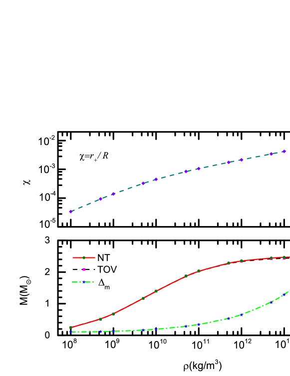
Figure 6: The general relativistic effect in charged white dwarfs, where the solid line and the dash-dot line in (b) represent the stellar masses under the framework of Newtonian gravity and the general relativity, respectively, while the green line in (b) represents the mass difference $\Delta_{m}$ between the two gravity theories, where $\alpha$=$5.0\times 10^{-19}$.

Table 1: $\alpha$, $R$, $M_{NT}/M_{\odot}$, $M_{TOV}/M_{\odot}$, $\Delta_{m}$, $\chi$ of the charged white dwarfs with $\rho_{c}=1.9\times 10^{13}kg/m^{3}$.

$\alpha$	$R(km)$	$M_{NT}/M_{\odot}$	$M_{TOV}/M_{\odot}$	$\Delta_{m}$	$\chi$
$8.6\times 10^{-19}$	$3754.8$	$58.4744$	$52.7244$	$0.09833$	$0.02959$
$8.5\times 10^{-19}$	$3355.3$	$41.7256$	$38.3719$	$0.08038$	$0.02426$
$8.3\times 10^{-19}$	$2839.9$	$25.3008$	$23.7974$	$0.05942$	$0.01816$
$8.0\times 10^{-19}$	$2389.3$	$15.0675$	$14.4134$	$0.04341$	$0.01353$
$7.5\times 10^{-19}$	$1975.3$	$8.5145$	$8.2523$	$0.03079$	$0.00985$
$7.0\times 10^{-19}$	$1735.1$	$5.7705$	$5.6293$	$0.02447$	$0.00798$
$6.5\times 10^{-19}$	$1575.6$	$4.3211$	$4.2317$	$0.02069$	$0.00683$
$6.0\times 10^{-19}$	$1461.4$	$3.4480$	$3.3853$	$0.01818$	$0.00607$
$5.7\times 10^{-19}$	$1407.2$	$3.0786$	$3.0261$	$0.01705$	$0.00572$
$5.5\times 10^{-19}$	$1375.6$	$2.8760$	$2.8288$	$0.01641$	$0.00552$
$5.0\times 10^{-19}$	$1309.2$	$2.4794$	$2.4419$	$0.01512$	$0.00511$
$4.5\times 10^{-19}$	$1256.8$	$2.1932$	$2.1621$	$0.01418$	$0.00480$
$4.0\times 10^{-19}$	$1214.8$	$1.9808$	$1.9542$	$0.01343$	$0.00456$
$3.5\times 10^{-19}$	$1181.1$	$1.8202$	$1.7970$	$0.01275$	$0.00436$
$3.0\times 10^{-19}$	$1154.0$	$1.6980$	$1.6771$	$0.01231$	$0.00421$
$2.0\times 10^{-19}$	$1115.8$	$1.5348$	$1.5168$	$0.01173$	$0.00400$
$1.0\times 10^{-19}$	$1094.6$	$1.4490$	$1.4325$	$0.01139$	$0.00389$
$1.0\times 10^{-20}$	$1087.9$	$1.4224$	$1.4064$	$0.01125$	$0.00385$

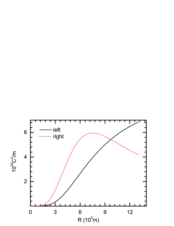
Figure 7: The values of the left hand and right hand of Eq.(36) as a function of $r$.

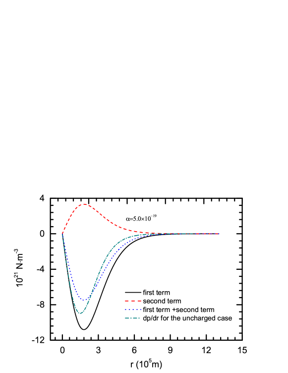
Figure 8: The right hand side terms of Eq. (32) with central density $\rho_{c}=1.9\times 10^{13}kg/m^{3}$ and $\alpha=5.0\times 10^{-19}$. The solid and dashed lines represent the first and second terms of right hand side of Eq. (32) respectively, the dotted line represents the overall effect of right hand side of Eq. (32), while the dot-dashed line represents $\frac{dp}{dr}$ of uncharged white dwarf ($\alpha=0$) with the same central density.

In the last section, the mass of charged white dwarf can reach up to $3M_{\odot}$, which is much larger than the Chandrasekhar mass limit. Thus it is natural to ask the validity of using Newtonian hydrostatic equilibrium equations. Does the general relativity effect become relevant and spoil all the results we obtained in the above section? In this section, we will try to answer these questions.

In general relativistic case, the spacetime outside of a charged white dwarf can be described by the Reissner-Nordstrom solution Weinberg72

$$ds^{2}=-\left(1-\frac{2GM}{c^{2}r}+\frac{GQ^{2}(r)}{4\pi\varepsilon_{0}c^{4}r^{2}}\right)dt^{2}+\left(1-\frac{2GM}{c^{2}r}+\frac{GQ^{2}(r)}{4\pi\varepsilon_{0}c^{4}r^{2}}\right)^{-1}dr^{2}+r^{2}\left(d\theta^{2}+\sin^{2}\theta d\varphi^{2}\right);$$ (30)

Usually, one use the quantity $\chi=\frac{r_{+}}{R}$ to indicate the significance of general relativity effects, here $R$ denotes radius of charged white dwarf, and $r_{+}=\frac{GM}{c^{2}}+\sqrt{\frac{G^{2}M^{2}}{c^{4}}-\frac{GQ^{2}}{4\pi\varepsilon_{0}c^{4}}}$ being the out horizon of Reissner-Nordstrom solution. When $\alpha=5.0\times 10^{-19}$, from the Fig. 7, we yield $\chi_{max}=0.00936$, which is very small, and hence in turn implies the general relativity effects in this case can be negligible. However, in order to justify this roughly estimates and concrete our result, we perform a detailed analysis on general relativity effects of charged white dwarf and to see how much it deviates from Newtonian dynamics. The interior line element of the static and spherical symmetric charged white dwarf reads

$$ds^{2}=-e^{\nu}dt^{2}+e^{\lambda}dr^{2}+r^{2}\left(d\theta^{2}+\sin^{2}\theta d\varphi^{2}\right),$$ (31)

where $\nu$ and $\lambda$ are only the function of radius $r$. And the classical hydrostatic equilibrium equations (1)-(3) should be replaced by Bekenstein71

$$\frac{dp}{dr}=-\frac{p+\rho c^{2}}{r(r-\frac{2Gm}{c^{2}}+\frac{Gq^{2}}{4\pi\varepsilon_{0}c^{4}r})}\left[\frac{4\pi G}{c^{4}}pr^{3}+\frac{Gm}{c^{2}}-\frac{Gq^{2}}{4\pi\varepsilon_{0}c^{4}r}\right]+\frac{qdq}{16\pi^{2}\varepsilon_{0}r^{4}dr},$$ (32)

$$\frac{dm}{dr}=4\pi r^{2}\rho+\frac{qdq}{4\pi\varepsilon_{0}c^{2}rdr},$$ (33)

and

$$q=\int_{0}^{r}4\pi\rho_{q}e^{\lambda/2}r^{2}dr,$$ (34)

where

$$e^{-\lambda}=1-\frac{2Gm(r)}{c^{2}r}+\frac{Gq^{2}(r)}{4\pi\varepsilon_{0}c^{4}r^{2}}.$$ (35)

By solving those equations numerically, we can compare our results with the Newtonian case. More specifically, we define a quantity $\Delta_{m}=\frac{M_{NT}-M_{TOV}}{M_{NT}}$, where $M_{NT}$ and $M_{TOV}$ represent the mass of white dwarf in the framework of Newtonian gravity and general relativity, respectively.

The numerical results are presented in Fig. 6 and Tab. 1. It is shown that the general relativity effect is indeed negligible when the mass of charged white dwarf smaller than $3M_{\odot}$. If we further increase the value of $\alpha$, the mass of corresponding charged white dwarf will became more higher, and the general relativistic effects will became relevant.

It is worthwhile to note that Bekenstein71 ; Prisco07 if the condition

$$\int^{r}_{0}\frac{q^{2}}{s^{2}}ds>\frac{q^{2}}{r}$$ (36)

is satisfied, the so called “active gravitational mass” Prisco07 will be increased, and hence contribute to the gravitational binding of the sphere. Then people natural wondering whether this interesting effect will decrease the effective mass of charged white dwarf? To illustrate this problem more clearly, we take a particular charged white dwarf with central matter density $\rho_{c}=1.9\times 10^{13}kg/m^{3}$ and $\alpha=5.0\times 10^{-19}$ as an example. From Fig. 7 we can see that when $r>9.70\times 10^{5}$$m$ the left hand side of Eq.(36) is larger than the right hand side, and thus implies the first term of right hand side of Eq.(32) becomes more negative. However, since the second term of the right hand side of Eq. (32) (i.e. $\frac{qdq}{16\pi^{2}\varepsilon_{0}r^{4}dr}$) is always positive. Therefore the gradient of pressure of charged white dwarf is less negative than the uncharged white dwarf when $r<2.42\times 10^{5}$$m$ as shown in Fig. 8. And this in turn ensure the mass of charged white dwarf with $\alpha=5.0\times 10^{-19}$ is uplifted to $2.44M_{\odot}$.

V Conclusions

In this paper, in order to explain some peculiar Type Ia supernova explosion, we propose a new mechanism based on the existence of charged white dwarf. Our calculations show that the mass of charged white dwarf can be uplifted significantly, and hence can naturally explain the observed peculiar Type Ia supernova explosion. Particularly, by employing a representative choice of charge distribution, we obtain an analytic solution for the stellar structure, as shown in Eq. (12). Then we continue to investigate the stability issue, the detailed calculations indicate that the charged white dwarf configuration is stable when the polytropic index $\gamma>\frac{4}{3}$. Since our treatment is based on Newtonian framework, to ensure the reliability of our results and also to explore the valid region of Newtonian framework, we further investigate the general relativistic effects. Our investigation shows that the general relativistic effects can be negligible when the mass of charged white dwarf is smaller than $3M_{\odot}$, and thus under this stellar mass the Newtonian framework is reliable.

It is worth noting that there are still many aspects of this theory deserving further investigation. For example, charge distribution other than Eq.(4) is of course allow in principle, can we find another charge distribution to reduce the total charge significantly? Furthermore, since we require the existence of very strong electric field in the charged white dwarf, is there any intrinsic observable effects induced by those strong electric field? We hope to back those issues in the near future.

- (1) D. A. Howell et al., The type Ia supernova SNLS-03D3bb from a super-chandrasekhar-mass white dwarf star, Nature (London) 443, 308 (2006).
- (2) R. A. Scalzo et al., Nearby supernova factory observations of SN 2007if: First total mass measurement of a super-Chandrasekhar-mass progenitor, Astrophys. J. 713, 1073 (2010).
- (3) M. Hicken, P. M. Garnavich, J. L. Prieto, S. Blondin, D. L. DePoy, R. P. Kirshner, and J. Parrent, The Luminous and Carbon-rich Supernova 2006gz: A Double Degenerate Merger?, Astrophys. J. 669, L17 (2007).
- (4) M. Yamanaka et al., Early phase observations of extremely luminous type Ia supernova 2009dc, Astrophys. J. 707, L118 (2009).
- (5) J. M. Silverman, M. Ganeshalingam, W. Li, A.V. Filippenko, A. A. Miller, and D. Poznanski, Exclusion of a luminous red giant as a companion star to the progenitor of supernova SN 2011fe, Mon. Not. R. Astron. Soc. 410, 585 (2011).
- (6) S. Taubenberger et al., High luminosity, slow ejecta and persistent carbon lines: SN 2009dc challenges thermonuclear explosion scenarios, Mon. Not. R. Astron. Soc. 412, 2735 (2011).
- (7) U. Das and B. Mukhopadhyay, Violation of Chandrasekhar mass limit: the exciting potential of strongly magnetized white dwarfs, Int. J. Mod. Phys. D 21, 1242001 (2012).
- (8) U. Das and B. Mukhopadhyay, Strongly magnetized cold degenerate electron gas: Mass-radius relation of the magnetized white dwarf, Phys. Rev. D 86, 042001 (2012).
- (9) U. Das and B. Mukhopadhyay, New Mass Limit for White Dwarfs: Super-Chandrasekhar Type Ia Supernova as a New Standard Candle, Phys. Rev. Lett. 110, 071102(2013).
- (10) J. M. Dong, W. Zuo, P. Yin, and J. Z. Gu, Comment on New Mass Limit for White Dwarfs: Super-Chandrasekhar Type Ia Supernova as a New Standard Candle , Phys. Rev. Lett. 112, 039001 (2014).
- (11) N. Chamel, A. F. Fantina, and P. J. Davis, Stability of super-Chandrasekhar magnetic white dwarfs, Phys. Rev. D 88, 081301(R), (2013).
- (12) J. G. Coelho, R. M. Marinho Jr., M. Malheiro, R. Negreiros, D. L. C ceres, J. A. Rueda, R. Ruffini, Dynamical instability of white dwarfs and breaking of spherical symmetry under the presence of extreme magnetic fields, arXiv:1306.4658.
- (13) U. Das, B. Mukhopadhyay, Revisiting some physics issues related to the new mass limit for magnetized white dwarfs, Mod. Phys. Lett. A 29, 1450035 (2014).
- (14) U. Das, B. Mukhopadhyay, Maximum mass of stable magnetized highly super-Chandrasekhar white dwarfs: stable solutions with varying magnetic fields, arXiv:1404.7627.
- (15) J. D. Bekenstein, Hydrostatic equilibrium and gravitational collapse of relativistic charged fluid balls, Phys. Rev. D 4, 2185 (1971).
- (16) D.D. Dionysiou, Equilibrium of a static charged perfect fluid sphere, Astrophys. Space. Sci. 85, 331 (1982).
- (17) S. Ray, A. L. Esp ndola, M. Malheiro, J. P. S. Lemos, and V. T. Zanchin, Electrically charged compact stars and formation of charged black holes, Phys. Rev. D 68, 084004 (2003)
- (18) C. R. Ghezzi, Relativistic structure, stability and gravitational collapse of charged neutron stars, Phys. Rev. D 72, 104017 (2005).
- (19) P. D. Lasky and A. W. C. Lun, Gravitational collapse of spherically symmetric plasmas in Einstein-Maxwell spacetimes, Phys. Rev. D 75, 104010 (2007)
- (20) R. P. Negreiros, F. Weber, M. Malheiro, and V. Usov, Electrically charged strange quark stars, Phys. Rev. D 80, 083006 (2009).
- (21) E. Olson, M. Bailyn, Charge effects in a static, spherically symmetric, gravitating fluid, Phys. Rev. D 13, 2204 (1976).
- (22) L. Herrera and W. Barreto, Newtonian polytropes for anisotropic matter: General framework and applications, Phys. Rev. D 87, 087303 (2013).
- (23) L. Herrera and W. Barreto, General relativistic polytropes for anisotropic matter: The general formalism and applications, Phys. Rev. D 88, 084022 (2013).
- (24) S. Weinberg, Gravitation and cosmology (John wiley, New York, 1972).
- (25) S. Chandrasekhar, E. Fermi, Problems of gravitational stability in the presence of a magnetic field, Astrophys. J. 118, 116 (1953)
- (26) A. I. Zhakin, Electrohydrodynamics, Phys. Usp. 55, 465 (2012).
- (27) A. Castellanos, Electrohydrodynamics, (Springer wien, New York, 1998).
- (28) A. Di Prisco, L. Herrera, G. Le Denmat, M. A. H. MacCallum, and N. O. Santos, Nonadiabatic charged spherical gravitational collapse, Phys. Rev. D 76, 064017 (2007).