Intensity Process for a Pure Jump Lévy Structural Model with Incomplete Information

Abstract  In this paper we discuss a credit risk model with a pure jump Lévy process for the asset value and an unobservable random barrier. The default time is the first time when the asset value falls below the barrier. Using the indistinguishability of the intensity process and the likelihood process, we prove the existence of the intensity process of the default time and find its explicit representation in terms of the distance between the asset value and its running minimal value. We apply the result to find the instantaneous credit spread process and illustrate it with a numerical example.

Keywords  Pure jump Lévy process, unobservable random barrier, first passage time, path-dependent intensity process.

Mathematics Subject Classification (2010)  60J75, 60G55, 91G40

1 Introduction

The structural model and the intensity model are two frameworks in credit risk modelling. The structural model is based on the asset-liability structure of a firm and is economically meaningful. The default time is defined as the first time the asset value process falls below the default threshold. One needs to investigate the law of the first passage time or equivalently the running minimal process. The intensity form model is based on the the fact that default happens as a surprise to the market and default time is a totally inaccessible stopping time under a certain filtration. One models directly the intensity process that determines the default indicator process and the short-term spread of credit derivatives such as defaultable bonds and credit default swaps.

The key difference of the two models is the difference of the information sets or filtrations, see Jarrow and Protter [11]. If the asset value process is continuous and the barrier is deterministic in a structural model with complete information, then the first passage time is a predictable stopping time and does not admit an intensity process under the natural filtration. In reality, it is difficult to observe the complete information of the asset value process and the default barrier. There has been active research in the literature on the filtration expansion and its applications in the structural model with incomplete information, see Guo and Zeng [9] and Janson et al. [10].

There are two main ways of introducing the incomplete information in the first passage time model in the literature. One is to assume the incomplete information about the value process and the constant barrier. Duffie and Lando [6] discuss for a discretely observable noisy value process and find the corresponding intensity process . Kusuoka [13] extends [6] to a continuously observable noisy value process. Çetin et al. [4] derive the intensity process with the Aézma martingale and the information reduction method. The other is to assume the observable asset value process but the incomplete information on the random barrier. Giesecke [7] introduces an unobservable random barrier and concludes that if the asset value is a diffusion process then the default time is a totally inaccessible stopping time under the market information filtration but does not admit an intensity process.

In this paper we focus on the first passage time problem of a structural model for a Lévy process with finite variation and with incomplete information of the barrier. Pure jump processes are important in financial modelling as they can capture the phenomenon of infinite activities, jumps, skewness and kurtosis. For example, Madan et al. [15] use a variance gamma process for the stock price in option pricing. Madan and Schoutens [18] use a drifted subordinator for the log firm value process in a first passage time model with complete information.

In the incomplete information setup the essential mathematical quantity needed is the conditional default probability. All results in the literature on the existence of the intensity process are based on the absolute continuity of the conditional default probability and the close link between the conditional default density and the intensity. In case of pure jump processes the conditional default probability is discontinuous at the time when the asset value process reaches a new minimal and the conditional default density does not exist. This is reasonable as one would expect the conditional default probability jumps when there is a large movement of the asset value process. The main mathematical difficulty, unlike the continuous case in which the compensator of the conditional default probability is itself, is to find the compensator due to the unpredictability of the stopping time.

The objective of the paper is to show that the structural model of a pure jump Lévy process with an unobservable random barrier can be embedded into an equivalent intensity model. The key contribution of the paper is to show the existence of the intensity process and find its explicit form for a pure jump Lévy process in an incomplete information framework, which sheds the new light to the relation between the intensity process of the default time and the running minimal process of the asset value. We apply the result to find the instantaneous credit spread process that remains positive and finite, which conforms to the market observations, and that depends on the historical path of the asset value.

The paper is organized as follows. Section 2 introduces the model, states the main result (Theorem 2.2) with several examples, and discusses the instantaneous credit spread with a numerical example. Section 3 proves the main result with details discussed in four subsections. Section 4 concludes.

2 The Model and the Main Result

Let $(\Omega,\mathcal{G},\mathbb{P})$ be a probability space and $V$ be an observable firm asset value process given by $V_{t}=V_{0}e^{X_{t}}$ at time $t$, where $X$ is a Lévy process with finite variation and $X_{0}=0$. Examples include drifted subordinators, variance gamma and normal inverse Gaussian processes. Note that $X$ can be decomposed as ([14, Exercise 2.8])

$$X_{t}=ct-S_{t}+S^{\prime}_{t},$$ (1)

where $c\in\mathbb{R}$ and $S$, $S^{\prime}$ are independent pure jump subordinators with Lévy measures $\pi$, $\pi^{\prime}$, respectively, see [14, Lemma 2.14] for the definition and the properties of a subordinator. Denote by $\mathbb{F}=(\mathcal{F}_{t})$ the natural filtration generated by $X$. We assume the following assumption be satisfied in the paper:

Assumption 2.1.

Lévy measure $\pi$ is continuous and satisfies $\int_{0}^{\infty}x\pi(dx)<\infty$.

Assume that the firm defaults at the first time when the asset value is below a default threshold, i.e., the default time $\tau$ is defined by

$$\tau:=\inf\{t>0:V_{t}\leq\tilde{D}\}=\inf\{t>0:X_{t}\leq D:=\ln(\tilde{D}/V_{0})\},$$

where $\tilde{D}$ is an unobservable default barrier of the company. Assume that $\tilde{D}$ is a uniform variable on the interval $[0,V_{0}]$ and is independent of $V$. Then the barrier $D$ for $X$ is a standard negative exponential variable, i.e., $-D$ is a standard exponential variable, with the distribution function $\mathbb{P}(D\leq x)=e^{x}$ for $x<0$, and is independent of $X$. Note that the default barrier is unobservable but the default time is observable, we therefore define a progressive filtration expansion $\mathbb{G}=(\mathcal{G}_{t})$ by ([16, Chapter VI, Section 3])

$$\mathcal{G}_{t}=\{B\in\mathcal{G}:\exists B_{t}\in\mathcal{F}_{t},B\cap\{\tau>t\}=B_{t}\cap\{\tau>t\}\}.$$ (2)

The default time $\tau$ is now a $\mathbb{G}$-stopping time. All filtrations involved are assumed to satisfy the usual condition.

Denote by $N$ the default indicator process, defined by $N_{t}:=\mathbf{1}_{\{\tau\leq t\}}$. The Doob-Meyer decomposition theorem implies that there exists a unique increasing predictable process $A$ with $A_{0}=0$, called the $\mathbb{G}$-compensator of $N$, such that $N-A$ is a $\mathbb{G}$-martingale. If $A$ is continuous a.s. then $\mathbb{G}$-stopping time $\tau$ is totally inaccessible. If $A$ is absolutely continuous a.s. with respect to the Lebesgue measure and $A$ can be written as $A_{t}=\int_{0}^{t}\lambda_{s}ds$ a.s., where $\lambda$ is nonnegative and $\mathbb{G}$-progressively measurable, then $\lambda$ is called the intensity process of $N$, see [3] for details on compensators and intensity processes.

Denote by $\pi(x+du):=\pi((x+u,x+u+du])$. If $\pi$ admits a Lévy density $\nu$, then $\pi(x+du)=\nu(x+u)dx$. We can now state the main result of the paper.

Theorem 2.2.

Let $X$ be a Lévy process with finite variation and Assumption 2.1 be satisfied. Then the $\mathbb{G}$-compensator of the default indicator process $N$ is absolutely continuous a.s. and the intensity process $\lambda$ of $N$ is indistinguishable with the instantaneous likelihood process $\tilde{\lambda}_{t}:=\lim_{h\downarrow 0}\frac{1}{h}\mathbb{P}(t<\tau\leq t+h|\mathcal{G}_{t})$ on $\{\tau>t\}$. Moreover, using the same notation as in (1), the intensity process $\lambda$ has the following representation

$$\lambda_{t}=\mathbf{1}_{\{\tau>t\}}\left(-c\mathbf{1}_{\{X_{t}-\underline{X}_{t}=0\}}\mathbf{1}_{\{c<0\}}+\Pi(X_{t}-\underline{X}_{t})\right),$$ (3)

where $\underline{X}_{t}:=\inf_{0\leq s\leq t}X_{s}$ is the running minimal process of $X$ and

$$\Pi(x):=\int_{0}^{\infty}(1-e^{-u})\pi(x+du),\quad\forall x\geq 0.$$ (4)

Theorem 2.2 shows that the intensity process $\lambda$ is an endogenous process that depends on the path of the asset value process $X$. Moreover, at each time $t$, $\lambda_{t}$ is a decreasing function of $X_{t}-\underline{X}_{t}$, a financially desirable property as it means that the default intensity increases when the asset value process $X$ approaches its historical minimal level.

We next give several examples to illustrate Theorem 2.2.

Example 2.3.

(Drifted Compound Poisson Process) Let $X$ be given by

$$X_{t}=ct-\sum_{i=1}^{M_{t}}Y_{i}+\sum_{i=1}^{M^{\prime}_{t}}Y^{\prime}_{i},$$

where $c\in\mathbb{R}$, $Y_{i}$ and $Y^{\prime}_{i}$ are exponential variables with parameters $\beta$ and $\beta^{\prime}$, respectively, $M$ and $M^{\prime}$ are Poisson processes with intensities $\rho$ and $\rho^{\prime}$, respectively, and $\{Y_{i}\}$, $\{Y^{\prime}_{i}\}$, $M$, $M^{\prime}$ are independent of each other. The Lévy density of $X_{t}$ on $\mathbb{R}_{-}$ is given by $\nu_{-}(x)=\rho\beta e^{-\beta x}$. The intensity process $\lambda$ of the default indicator process $N$ is then given by Theorem 2.2 as

$$\lambda_{t} = \mathbf{1}_{\{\tau>t\}}\left(-c\mathbf{1}_{\{X_{t}-\underline{X}_{t}=0\}}\mathbf{1}_{\{c<0\}}+\frac{\rho}{1+\beta}e^{-\beta(X_{t}-\underline{X}_{t})}\right).$$

Example 2.4.

(Drifted Gamma Process) Let $X$ be given by

$$X_{t}=ct-G_{t},$$

where $c>0$, $G_{t}$ is a gamma process $\Gamma(t,\mu,\nu)$ with the mean rate $\mu$, the variance rate $\nu$, and the Lévy density $\nu(x)=\frac{\mu^{2}}{\nu}e^{-\frac{\mu}{\nu}x}x^{-1}$. The intensity process of $N$ is given by

$$\lambda_{t}=\mathbf{1}_{\{\tau>t\}}\left(\int_{0}^{\infty}(1-e^{-u})\frac{\mu^{2}}{\nu}e^{-\frac{\mu}{\nu}(u+X_{t}-\underline{X}_{t})}(u+X_{t}-\underline{X}_{t})^{-1}du\right).$$

Note that $c>0$ in this case, hence the first term in (3) disappears.

Example 2.5.

(Variance Gamma Process [15]) Let $X$ be a variance gamma process $VG(c,\nu,\sigma,\theta)$ that is generated by a drifted Brownian motion $\theta t+\sigma W_{t}$, time-changed by a gamma process $\Gamma(t;1,\nu)$, and an additional drift term $ct$, then

$$X_{t}=ct+\Gamma(t;\mu_{+},\nu_{+})-\Gamma(t;\mu_{-},\nu_{-}),$$ (5)

where $\mu_{\pm}=\frac{1}{2}\sqrt{\theta^{2}+\frac{2\sigma^{2}}{\nu}}\pm\frac{\theta}{2}$, and $\nu_{\pm}=\mu_{\pm}^{2}\nu$. The intensity process of $N$ is given by

$$\lambda_{t}=\mathbf{1}_{\{\tau>t\}}\left(-c\mathbf{1}_{\{X_{t}-\underline{X}_{t}=0\}}\mathbf{1}_{\{c<0\}}+\int_{0}^{\infty}(1-e^{-u})\frac{(\mu_{-})^{2}}{\nu_{-}}e^{-\frac{\mu_{-}}{\nu_{-}}(u+X_{t}-\underline{X}_{t})}(u+X_{t}-\underline{X}_{t})^{-1}du\right).$$ (6)

We next provide an application of Theorem 2.2 in credit risk modelling. The credit spread $S(t,h)$ of a defaultable name over the time interval $[t,t+h]$ is defined by

$$S(t,h):=-\frac{1}{h}\ln\left(1-\mathbb{P}(t<\tau\leq t+h|\mathcal{G}_{t})\right),$$

where $\mathbb{P}\left(t<\tau\leq t+h|\mathcal{G}_{t}\right)$ is the conditional default probability given $\tau>t$. Using the Taylor expansion, we can find the instantaneous credit spread $s(t)$ as

$$s(t):=\lim_{h\downarrow 0}S(t,h)=\lim_{h\downarrow 0}\frac{1}{h}\mathbb{P}\left(t<\tau\leq t+h|\mathcal{G}_{t})\right)=\tilde{\lambda}_{t}.$$

Theorem 2.2 says that $s(t)$ is positive and finite almost surely and is given by

$$s(t)=-c\mathbf{1}_{\{X_{t}-\underline{X}_{t}=0\}}\mathbf{1}_{\{c<0\}}+\Pi(X_{t}-\underline{X}_{t}),$$

which conforms to the market observation that the instantaneous credit spread remains positive and finite even though the bond is near its maturity and that the bond price often drops around the time of default due to uncertainties about the closeness of the current asset value to the default threshold. For more details of the instantaneous credit spread and its term structure, see [6, 7].

We next give a numerical example to illustrate the results. We take the variance gamma process $VG(c,\nu,\sigma,\theta)$ in Example 2.5. The data used are $(c,\nu,\sigma,\theta)=(-0.02,0.1,0.15,0.01)$. Figure 2.1 displays for $t\in[0,5]$ a sample path of the asset return process $X$, the running minimal process $\underline{X}$ and the resulting intensity process $\lambda$. Figure 2.1 also shows the distance $X_{t}-\underline{X}_{t}$ and its contribution $\Pi(X_{t}-\underline{X}_{t})$ to the intensity. We can observe the reciprocal relation of the intensity $\lambda_{t}$ and the distance $X_{t}-\underline{X}_{t}$, which is consistent with the observation in the credit market. Note that $\Pi(\cdot)$ on $\mathbb{R}_{+}$ is bounded above by $\Pi(0)$ that is fully determined by the Lévy measure of $X$. The upper bound $\Pi(0)$ is reached when $X_{t}-\underline{X}_{t}=0$, i.e. the process $X$ reaches a new minimal level, and the intensity $\lambda_{t}$ at that time is above $\Pi(0)$ by the amount $|c|$ as the drift parameter $c<0$. Figure 2.2, using the same sample path of Figure 2.1, shows the term structure of the credit spread $h\mapsto S(t,h)$ at time $t=0.5$, starting from $S(t,0)=\lambda_{t}$.

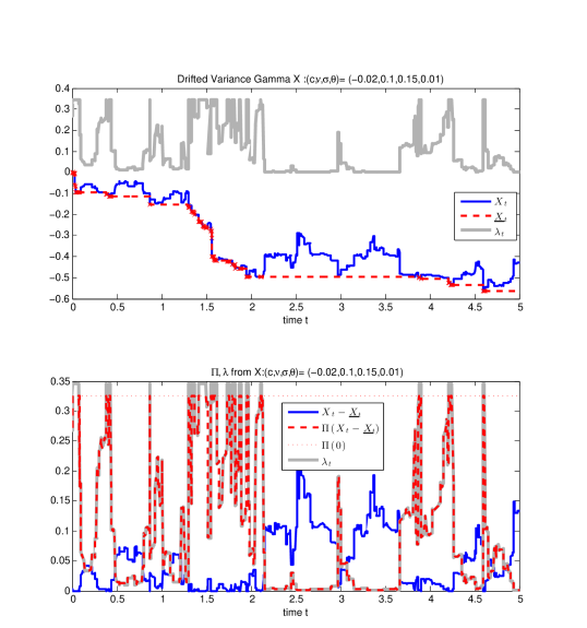
Figure 2.1: The asset return process $X$ as in Example 2.5, the distance process $X-\underline{X}$ and the intensity process $\lambda$. The data used are $(c,\nu,\sigma,\theta)=(-0.02,0.1,0.15,0.01)$.

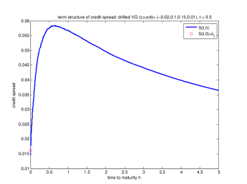
Figure 2.2: The term structure of credit spread $S(t,h)$: the asset return process $X$ as in Example 2.5 with the data $(c,\nu,\sigma,\theta)=(-0.02,0.1,0.15,0.01)$, at $t=0.5$, $X_{t}-\underline{X}_{t}=0.0585$.

3 Proof of Theorem 2.2

Theorem 2.2 is proved in four steps, detailed in the following subsections. Subsection 3.1 shows the relation of the likelihood processes under different filtration (Lemma 3.2), Subsections 3.2 and 3.3 establish the existence of the limit process for a spectrally negative Lévy process with finite variation (Proposition 3.8) and for a general Lévy process with finite variation (Proposition 3.11), and Subsection 3.4 confirms the indistinguishability of the instantaneous likelihood process and the intensity process using Aven’s condition.

3.1 Compensators and Likelihood Processes under Different Filtrations

The conditional survival probability at each time $t$ is given by

$$Z_{t}:=\mathbb{P}(\tau>t|\mathcal{F}_{t})=\mathbb{P}(\underline{X}_{t}>D|\mathcal{F}_{t})=e^{\underline{X}_{t}}.$$

It is known ([16, Chapter VI, Theorem 11]) that there exists a unique, increasing, $\mathbb{G}$-predictable process $A$, the $\mathbb{G}$-compensator of $N$, such that the difference of $A$ and $N$ is a uniformly integrable $\mathbb{G}$-martingale. Our objective is to find $A$.

Let $Z_{t-}=\lim_{s\uparrow t}Z_{s}$ and $Z_{0-}=1$. Define a nondecreasing $\mathbb{F}$-predictable process $A$ by

$$A_{t}=\int_{0}^{t}\frac{dK_{s}}{Z_{s-}},$$

where $K_{t}$ is the unique, increasing, $\mathbb{F}$-predictable compensator of $\mathbb{F}$-submartingale $1-Z_{t}=\mathbb{P}(\tau\leq t|\mathcal{F}_{t})$.

Theorem 3.1 ([12]).

The process $N-A^{\tau}$ is a $\mathbb{G}$-martingale, where $A^{\tau}=(A_{t\wedge\tau})_{t\geq 0}$.

Theorem 3.1 shows that one can transform the problem of finding the $\mathbb{G}$-compensator of $N$ into the problem of finding the $\mathbb{F}$-compensator of $Z$. If $Z_{t}$ is a continuous process, then $K_{t}=-Z_{t}$ and $A_{t}=-\ln(Z_{t})$. If $Z$ is discontinuous, then finding $K$ is nontrivial, see [9].

The next result characterizes the likelihood processes under different filtrations.

Lemma 3.2.

For any Lévy process $X$, $h>0$, denote

$$k^{h}_{t} := \frac{1}{h}\mathbb{E}\left[K_{t+h}-K_{t}|\mathcal{F}_{t}\right]\quad\mbox{and}\quad\lambda^{h}_{t}:=\frac{1}{h}\mathbb{E}\left[N_{t+h}-N_{t}|\mathcal{G}_{t}\right].$$

Then,

$$k^{h}_{t}=e^{\underline{X}_{t}}\frac{1}{h}\mathbb{E}\left[1-e^{-\left(y-\underline{X}_{h}\right)^{+}}\right]\Big{|}_{y=\underline{X}_{t}-X_{t}}\quad\mbox{and}\quad\lambda^{h}_{t}=1_{\{\tau>t\}}e^{-\underline{X}_{t}}k^{h}_{t}.$$ (7)

Proof.

Since

$$\underline{X}_{t+h}-\underline{X}_{t} = \inf_{u\in[t,t+h]}X_{u}\wedge\underline{X}_{t}-\underline{X}_{t}$$

$$= \inf_{u\in[0,h]}(X_{t+u}-X_{t})\wedge(\underline{X}_{t}-X_{t})-(\underline{X}_{t}-X_{t})$$

$$= -\left((\underline{X}_{t}-X_{t})-\inf_{u\in[0,h]}(X_{t+u}-X_{t})\right)^{+},$$

we have

$$\mathbb{E}\left[e^{\underline{X}_{t+h}}-e^{\underline{X}_{t}}|\mathcal{F}_{t}\right] = e^{\underline{X}_{t}}\mathbb{E}\left[e^{\underline{X}_{t+h}-\underline{X}_{t}}-1|\mathcal{F}_{t}\right]$$

$$= e^{\underline{X}_{t}}\mathbb{E}\left[e^{-\left((\underline{X}_{t}-X_{t})-\inf_{u\in[0,h]}(X_{t+u}-X_{t})\right)^{+}}-1|\mathcal{F}_{t}\right]$$

$$= e^{\underline{X}_{t}}\mathbb{E}\left[e^{-\left(y-\underline{X}_{h}\right)^{+}}-1\right]\Big{|}_{y=\underline{X}_{t}-X_{t}},$$

where the last equality comes from the independent and stationary increment property of Lévy process $X$ and adaptedness of $X$ and $\underline{X}$ in $\mathbb{F}$. Since $K$ is the $\mathbb{F}$-compensator of $1-Z$, the Doob-Meyer decomposition says that

$$\mathbb{E}\left[K_{t+h}-K_{t}|\mathcal{F}_{t}\right]=-\mathbb{E}\left[Z_{t+h}-Z_{t}|\mathcal{F}_{t}\right]=-\mathbb{E}\left[e^{\underline{X}_{t+h}}-e^{\underline{X}_{t}}|\mathcal{F}_{t}\right].$$

Combining the above gives $k^{h}_{t}$ in (7).

Next, by the optional projection theorem (Theorem 14, Chap.VI, [16] and [7]), we know that if a random variable $\xi$ is nonnegative and integrable, then for each $t\geq 0$, the right continuous version of $\mathbb{E}[\xi|\mathcal{G}_{t}]$ is given by

$$\mathbb{E}[\xi|\mathcal{G}_{t}]=1_{\{\tau>t\}}\frac{1}{Z_{t}}\mathbb{E}\left[\xi 1_{\{\tau>t\}}|\mathcal{F}_{t}\right]+\xi 1_{\{\tau\leq t\}}\quad a.s.$$ (8)

Therefore, using the tower property of the expectation and the fact that $K$ is a $\mathbb{F}$-compensator of $1-Z$, we have

$$\lambda^{h}_{t} = \frac{1}{h}\mathbb{E}\left[N_{t+h}-N_{t}|\mathcal{G}_{t}\right]$$

$$= 1_{\{\tau>t\}}\frac{1}{h}{1\over Z_{t}}\mathbb{E}\left[1_{\{t<\tau\leq t+h\}}|\mathcal{F}_{t}\right]$$

$$= 1_{\{\tau>t\}}\frac{1}{h}\frac{1}{Z_{t}}\mathbb{E}\left[Z_{t}-Z_{t+h}|\mathcal{F}_{t}\right]$$

$$= 1_{\{\tau>t\}}\frac{1}{Z_{t}}\frac{1}{h}\mathbb{E}\left[K_{t+h}-K_{t}|\mathcal{F}_{t}\right].$$

$$= 1_{\{\tau>t\}}e^{-\underline{X}_{t}}k^{h}_{t}.$$

This gives $\lambda^{h}_{t}$ in (7).∎

The next result follows immediately from Lemma 3.2.

Corollary 3.3.

Assume that $\tilde{k}_{t}:=\lim_{h\downarrow 0}k^{h}_{t}$ exists for all $t$ a.s., then the instantaneous likelihood process on $\{\tau>t\}$ is given by

$$\tilde{\lambda}_{t}:=\lim_{h\downarrow 0}\frac{1}{h}\mathbb{P}(t<\tau\leq t+h|\mathcal{G}_{t})=e^{-\underline{X}_{t}}\tilde{k}_{t}.$$

Remark 3.4.

Note that $\xi 1_{\{\tau\leq t\}}$ in (8) is $\mathcal{G}_{t}$ measurable by definition. Indeed, since $\xi$ and $\tau$ are random variables on $(\Omega,\mathcal{G},\mathbb{P})$, then $\xi 1_{\{\tau\leq t\}}$ is $\mathcal{G}$-measurable. To show it is $\mathcal{G}_{t}$ measurable, it is equivalent to show $\forall b\in\mathbb{R},\quad B(b):=\{\omega:\xi(\omega)1_{\{\tau\leq t\}}(\omega)\leq b\}\in\mathcal{G}_{t}$. Note that

$$B(b)\cap\{t<\tau\} = \{\xi 1_{\{\tau\leq t\}}\leq b\}\cap\{t<\tau\}$$

$$= \left(\{\xi\leq b,\tau\leq t\}\cup\{0\leq b,t<\tau\}\right)\cap\{t<\tau\}$$

$$= \{0\leq b,t<\tau\}$$

$$= 1_{\{b<0\}}\emptyset+1_{\{b\geq 0\}}\{t<\tau\}$$

$$= 1_{\{b<0\}}\left(\emptyset\cap\{t<\tau\}\right)+1_{\{b\geq 0\}}\left(\Omega\cap\{t<\tau\}\right).$$

Since $\emptyset,\Omega\in\mathcal{F}_{t}$ for all $t\geq 0$, we can take $B_{t}(b):=1_{\{b<0\}}\emptyset+1_{\{b\geq 0\}}\Omega\in\mathcal{F}_{t}$, such that

$$B(b)\cap\{\tau>t\}=B_{t}(b)\cap\{\tau>t\}.$$

Therefore, we have $B(b)\in\mathcal{G}_{t}$.

3.2 Spectrally Negative Lévy Process with Finite Variation

Let $X$ be a spectrally negative Lévy process with finite variation, then $X$ has a representation [14, page 56]

$$X_{t}=ct-S_{t},$$ (9)

where $c>0$ and $S$ is a pure jump subordinator with Lévy measure $\pi$. (9) is a special case of (1) with $\pi^{\prime}=0$ and $c>0$. The Lévy measure of $X$ is $\pi_{X}(dx)=\pi(d(-x))=\pi((-x,-x+dx])$ on $\mathbb{R}_{-}$ and if $\pi$ admits a density $\nu$ then $\pi(-dx)=\nu(-x)dx$. The following concept is needed in analysing the path property of $\underline{X}$.

Definition 3.5 ([14]).

Let $X$ be a Lévy process. A point $x\in\mathbb{R}$ is said to be irregular for an open or closed set $B$ if $\mathbb{P}_{x}\left(\tau^{B}=0\right)=0$, where the stopping time $\tau^{B}=\inf\{t>0:X_{t}\in B\}$.

We know ([5, Chapter 9, Proposition 15]) that for $X$ defined in (9), $0$ is irregular for $(-\infty,0)$. Hence, starting at $0$, it takes $X$ strictly positive time to reach $(-\infty,0)$. If we define $T_{1}:=\inf\{t>0:X_{t}<0\}$, then $\mathbb{P}(T_{1}>0)=1$. $T_{1}$ is the first jump time of $\underline{X}$ but may not be the first jump time of $X$. We observe that $\underline{X}$ is a pure-jump process as $\underline{X}$ can only move when $S$ jumps and $\underline{X}$ cannot jump to a pre-specified level on $(-\infty,0)$ as $X$ can not, see [14, Exercise 5.9]. Hence, the jump size of $\underline{X}$ has no atoms and is strictly negative. The number of jumps of $\underline{X}$ on the interval $[0,t]$, i.e., $n_{t}:=\#\{s\in(0,t]:X_{s}=\underline{X}_{s}\}$, is a discrete set and is a.s. finite. Moreover, we denote the arrival times of $n_{t}$ by $(T_{i})_{i}$, the inter-arrival times by $(\delta_{i})_{i}$, and the jump sizes by $(\xi_{i})_{i}$. Then we have the following lemma.

Lemma 3.6.

For $X$ defined in (9), $\underline{X}$ can be written as a renewal-reward process

$$\underline{X}_{t}=-\sum_{i=1}^{n_{t}}\xi_{i},$$

where $(\delta_{i},\xi_{i})$ are i.i.d. random variables.

Proof.

The analysis above shows that $\underline{X}$ is a non-explosive marked point process and can be written as $\underline{X}_{t}=-\sum_{i=1}^{n_{t}}\xi_{i}$, where $-\xi_{i}=\Delta\underline{X}_{T_{i}}=\underline{X}_{T_{i}}-\underline{X}_{T_{i-1}}=X_{T_{i}}-X_{T_{i-1}}$. Since $(T_{i})_{i}$ are also jump times of Lévy process $X$ and are stopping-times. We have that $(\delta_{i},\xi_{i})_{i}$ are i.i.d. random variables due to the strong Markov property of $X$. ∎

Instead of investigating the exact law of $\underline{X}$, we only need to analyse the small-time behaviour of the process, which can be done with the help of the next result, called the Ballot Theorem [2, Proposition 2.7].

Lemma 3.7 ([2]).

Let $X$ be defined in (9) and $T_{1}:=\inf\{t>0:X_{t}<0\}$. Then, for every $t>0$, $z\geq 0$, and $u<-z$,

$$\mathbb{P}\left(T_{1}\in dt,X_{T_{1}-}\in dz,\Delta X_{T_{1}}\in du\right)=\frac{z}{ct}\mathbb{P}(X_{t}\in dz)\pi(-du)dt,$$

where $\Delta X_{t}=X_{t}-X_{t-}$ and $\pi$ is the Lévy measure of $S$.

Hence the joint distribution of $(T_{1},X_{T_{1}})$ is given by

$$\mathbb{P}(T_{1}\in dt,X_{T_{1}}\in dw) = \left(\int_{z\in(0,\infty)}z\pi(z+d(-w))\mathbb{P}(X_{t}\in dz)\right)\frac{1}{ct}dt$$ (10)

for $w\leq 0$. The following is another version of the Ballot theorem:

$$\mathbb{P}(T_{1}>t,X_{t}\in dx)=\frac{x}{ct}\mathbb{P}(X_{t}\in dx)$$

for every $t>0$ and $x\in[0,\infty)$. Since $X_{t}=ct-S_{t}\leq ct$, we have

$$\mathbb{P}(T_{1}>t)=\frac{1}{ct}\int_{0}^{\infty}x\mathbb{P}(X_{t}\in dx)=\frac{1}{ct}\int_{0}^{ct}x\mathbb{P}(X_{t}\in dx)=\frac{1}{c}\mathbb{E}\left[\mathbf{1}_{\{0\leq X_{t}\leq ct\}}\frac{X_{t}}{t}\right].$$

Note as $\lim_{t\downarrow 0}\frac{S_{t}}{t}=0$ a.s., we have for almost all $\omega$, there exists $t_{0}(\omega)$, such that for all $t\in[0,t_{0}(\omega)]$, $S_{t}(\omega)\leq ct$, hence $0\leq X_{t}(\omega)=ct-S_{t}(\omega)\leq ct$ and

$$\lim_{t\downarrow 0}\mathbf{1}_{\{0\leq X_{t}\leq ct\}}=1\quad a.s.$$ (11)

The dominated convergence theorem leads to

$$\lim_{t\downarrow 0}\mathbb{P}(T_{1}>t)=\frac{1}{c}\mathbb{E}\left[\lim_{t\downarrow 0}\mathbf{1}_{\{0\leq X_{t}\leq ct\}}\frac{X_{t}}{t}\right]=\frac{1}{c}\cdot c=1.$$ (12)

Proposition 3.8.

Let $X$ be defined in (9) and let Assumption 2.1 be satisfied. Then the following limit exists for all $t$ a.s.

$$\tilde{k}_{t}:=\lim_{h\downarrow 0}k^{h}_{t}=e^{\underline{X}_{t}}\Pi(X_{t}-\underline{X}_{t}),$$

where $k_{t}^{h}$ is defined in (7) for $h>0$ and $\Pi$ is defined in (4).

Proof.

Recall that $\underline{X}_{t}=-\sum_{i=1}^{n_{t}}\xi_{i}$ is a renewal-reward process, where jump size $\xi_{i}$ and inter-arrival times $\delta_{i}$ are positive random variables for all $i$, and $(\delta_{i},\xi_{i})$ are i.i.d. random variables.

By (12), denote by $F$ the distribution function of $\delta_{i}$. Then

$$\lim_{t\downarrow 0}F(t)=\lim_{t\downarrow 0}P(T_{1}\leq t)=0=F(0).$$

Hence, $F$ is right continuous at zero, i.e. $F(0)=F(0+)=0$.

Denote by, for $t>0$ and $y\leq 0$,

$$\Lambda^{0}_{t}(y) := \frac{1}{t}\mathbb{E}\left[1-e^{-(y-\underline{X}_{t})^{+}}\right]$$

$$\Lambda_{t}^{1}(y) := \frac{1}{t}\mathbb{E}\left[1_{\{n_{t}=1\}}(1-e^{-(\xi_{1}+y)^{+}})\right]$$

$$\Lambda_{t}^{2}(y) := \frac{1}{t}\mathbb{E}\left[\sum_{k=2}^{\infty}1_{\{n_{t}=k\}}\left(1-e^{-\left(\sum_{i=1}^{k}\xi_{i}+y\right)^{+}}\right)\right].$$

We have

$$\Lambda^{0}_{t}(y)=\mathbb{E}\left[1-e^{-\left(y+\sum_{i=1}^{n_{t}}\xi_{i}\right)^{+}}\right]=\Lambda^{1}_{t}(y)+\Lambda^{2}_{t}(y).$$

We next show that for $y\leq 0$,

$$\lim_{t\rightarrow 0}\Lambda^{1}_{t}(y)=\Pi(-y),\mbox{ and }\lim_{t\rightarrow 0}\Lambda^{2}_{t}(y)=0.$$ (13)

Then, (13) gives the required conclusion.

Since $\delta_{1}$ and $\delta_{2}$ are independent, also noting (10), we have

$$\mathbb{E}\left[1_{\{n_{t}=1\}}(1-e^{-(\xi_{1}+y)^{+}})\right]$$

$$= \mathbb{E}\left[1_{\{T_{1}\leq t\}}1_{\{T_{2}-T_{1}>t-T_{1}\}}(1-e^{-(\xi_{1}+y)^{+}})\right]$$

$$= \int_{0}^{t}\int_{-y}^{\infty}\bar{F}_{T_{1}}(t-s)(1-e^{-x-y})\mathbb{P}(T_{1}\in ds,X_{T_{1}}\in d(-x))$$

$$= \int_{s=0}^{t}\int_{x=-y}^{\infty}\bar{F}_{T_{1}}(t-s)(1-e^{-x-y})\left(\int_{z=0}^{\infty}z\pi(z+dx))\mathbb{P}(X_{s}\in dz)\right)\frac{1}{cs}ds$$

$$= \frac{1}{c}\int_{s=0}^{t}\bar{F}_{T_{1}}(t-s)\int_{z=0}^{\infty}\left(\int_{u=0}^{\infty}(1-e^{-u})\pi(z-y+du)\right)z\frac{\mathbb{P}(X_{s}\in dz)}{s}ds$$

$$= \frac{1}{c}\int_{s=0}^{t}\bar{F}_{T_{1}}(t-s)\left(\int_{z=0}^{cs}\Pi(z-y)z\frac{\mathbb{P}(X_{s}\in dz)}{s}\right)ds.$$

The last equality is due to $X_{s}=cs-S_{s}\leq cs$.

Since $S$ is a pure jump subordinator, we have ([14, Lemma 4.11]) $\lim_{t\rightarrow 0}\frac{S_{t}}{t}=0\quad\mbox{a.s.}$, which implies

$$\lim_{t\rightarrow 0}\frac{X_{t}}{t}=c.$$ (15)

Using (15) and (11), the dominated convergence theorem, continuity of $\Pi(\cdot)$, and $X_{0+}=0$, we obtain

$$\lim_{s\downarrow 0}\int_{z=0}^{cs}z\Pi(z-y)\frac{\mathbb{P}(X_{s}\in dz)}{s} = \lim_{s\downarrow 0}\mathbb{E}\left[1_{\{0\leq X_{s}\leq cs\}}\frac{X_{s}}{s}\Pi(X_{s}-y)\right]$$

$$= \mathbb{E}\left[\lim_{s\downarrow 0}1_{\{0\leq X_{s}\leq cs\}}\frac{X_{s}}{s}\Pi(X_{s}-y)\right]$$

$$= c\Pi(-y).$$

Taking the limit in (3.2) gives

$$\lim_{t\downarrow 0}\Lambda_{t}^{1}(y)=\frac{1}{c}\lim_{s\downarrow 0}\int_{z=0}^{cs}z\Pi(z-y)\frac{\mathbb{P}(X_{s}\in dz)}{s}=\Pi(-y).$$

Here we have used the fact that if $g(\cdot)$ is a nonnegative function and $\bar{F}(0+)=1$, then

$$\frac{1}{t}\int_{0}^{t}\bar{F}(t)g(s)ds\leq\frac{1}{t}\int_{0}^{t}\bar{F}(t-s)g(s)ds\leq\frac{1}{t}\int_{0}^{t}g(s)ds$$

and

$$\lim_{t\rightarrow 0}\frac{1}{t}\int_{0}^{t}\bar{F}(t-s)g(s)ds=\lim_{t\rightarrow 0}\frac{1}{t}\int_{0}^{t}g(s)ds=g(0+).$$

We have proved the first limit in (13). We next prove the second limit in (13). Since

$$\Lambda^{0}_{t}(0)=\frac{1}{t}\mathbb{E}\left[1-e^{\underline{X}_{t}}\right]\leq\frac{1}{t}\mathbb{E}\left[1-e^{-S_{t}}\right]=\frac{1}{t}\left(1-e^{-\Pi(0)t}\right)\leq\Pi(0)$$

and

$$0\leq\Lambda^{1}_{t}(0)\leq\Lambda^{0}_{t}(0)\leq\Pi(0),$$

the first limit in (13) implies

$$\lim_{t\rightarrow 0}\Lambda^{0}_{t}(0)=\lim_{t\rightarrow 0}\Lambda^{1}_{t}(0)=\Pi(0),$$

therefore

$$\lim_{t\rightarrow 0}\Lambda^{2}_{t}(0)=0.$$

On the other hand, we know

$$0\leq\Lambda^{2}_{t}(y)\leq\Lambda^{2}_{t}(0)\quad\mbox{for all $y\leq 0$},$$

which proves the second limit in (13). Hence, $\Lambda^{0}_{t}(y)=\Pi(-y)$ and $\tilde{\lambda}_{t}=\Lambda^{0}_{t}(X_{t}-\underline{X}_{t})=\Pi(X_{t}-\underline{X}_{t})$. ∎

Remark 3.9.

Note that $\Pi(\cdot)$ is continuous as $\pi(dx)$ is. $\Pi(0)=-\ln\mathbb{E}[e^{-S_{1}}]$ is the Laplace exponent of $S$ from the Lévy-Khintchine formula, and $0<\Pi(x)\leq\Pi(0)<\int_{0}^{\infty}u\pi(du)<\infty$ for all $x\geq 0$ by Assumption 2.1. Therefore, $\Pi$ is bounded on $\mathbb{R}_{+}.$

3.3 Lévy Process with Finite Variation

Suppose $X$ is a Lévy process with finite variation. It then has a representation (1) and we assume that Assumption 2.1 holds. Note that the path properties and techniques used in Subsection 3.2 no longer hold. In (1), denote the drift and negative jump components as

$$Z_{t}(c):=ct-S_{t}.$$

Then we first claim the following result for $Z_{t}(c)$.

Lemma 3.10.

For any $c\in\mathbb{R}$ and $y\leq 0$ the following limit exists:

$$\lim_{h\rightarrow 0}\frac{1}{h}\mathbb{E}\left[1-e^{-(y-\underline{Z}_{h}(c))^{+}}\right] = -c\mathbf{1}_{\{y=0\}}\mathbf{1}_{\{c<0\}}+\Pi(-y),$$ (16)

where $\Pi$ is defined in (4).

Proof.

For $c>0$ the limit (16) has been proved in the previous subsection. We now consider the case of $c\leq 0$. Note that $Z_{h}(c)$ is decreasing in $h$ and $\underline{Z}_{h}(c)=Z_{h}(c)$. We split the proof into two cases.

(i) $y=0$: We have

$$\lim_{h\rightarrow 0}\frac{1}{h}\mathbb{E}\left[1-e^{-(y-\underline{Z}_{h}(c))^{+}}\right]=\lim_{h\rightarrow 0}\frac{1}{h}\mathbb{E}\left[1-e^{ch-S_{h}}\right] = -c+\Pi(0).$$

(ii) $y<0$: Take the function $f(x):=1-e^{-(y+x)^{+}}$ which is bounded, continuous, and vanishes in a neighbourhood of zero: take $\epsilon<-y$, then for any $x\in(0,\epsilon)$, we have $f(x)=0$. Hence

$$\lim_{h\rightarrow 0}\frac{1}{h}\mathbb{E}\left[1-e^{-(y-\underline{Z}_{h}(c))^{+}}\right] = \lim_{h\rightarrow 0}\frac{1}{h}\mathbb{E}\left[f(-Z_{h}(c))\right]=\int_{\mathbb{R}}f(x)\pi(dx).$$

The second equality is due to [17, Corollary 8.9] and $\pi$ being the Lévy measure of $-Z_{h}(c)$. Therefore,

$$\int_{\mathbb{R}}f(x)\pi(dx) = \int_{-y}^{\infty}(1-e^{-(y+x)})\pi(dx)=\int_{0}^{\infty}(1-e^{-u})\pi(-y+du)=\Pi(-y),$$

which proves (16). ∎

Proposition 3.11.

Let $X_{t}$ be defined in (1) and let Assumption 2.1 be satisfied. Then the following limit exists for all $t$ a.s.

$$\tilde{k}_{t}:=\lim_{h\downarrow 0}k^{h}_{t}=e^{\underline{X}_{t}}\left(-c\mathbf{1}_{\{X_{t}-\underline{X}_{t}=0\}}\mathbf{1}_{\{c<0\}}+\Pi(X_{t}-\underline{X}_{t})\right),$$ (17)

where $k_{t}^{h}$ is defined in (7) for $h>0$ and $\Pi$ is defined in (4). The instantaneous likelihood process $\tilde{\lambda}_{t}$ defined in Corollary 3.3 is given by

$$\tilde{\lambda}_{t}=-c\mathbf{1}_{\{X_{t}-\underline{X}_{t}=0\}}\mathbf{1}_{\{c<0\}}+\Pi(X_{t}-\underline{X}_{t}).$$ (18)

Proof.

The expression of $\tilde{\lambda}_{t}$ in (18) is an immediate result of Corollary 3.3 and (17). To prove (17) we only need to show that for all $y\leq 0$,

$$\lim_{h\rightarrow 0}\frac{1}{h}\mathbb{E}\left[1-e^{-(y-\underline{X}_{h})^{+}}\right]=-c\mathbf{1}_{\{y=0\}}\mathbf{1}_{\{c<0\}}+\Pi(-y).$$ (19)

Since $f(x)=1-e^{-(y-x)^{+}}$ is a decreasing function of $x$ on $\mathbb{R}_{-}$ and $X_{h}=ch-S_{h}+S^{\prime}_{h}\geq ch-S_{h}=Z_{h}(c)$ for all $\omega$ and $h>0$, we have $\underline{X}_{h}\geq\underline{Z}_{h}(c)$ and

$$\frac{1}{h}\mathbb{E}\left[1-e^{-(y-\underline{X}_{h})^{+}}\right] \leq \frac{1}{h}\mathbb{E}\left[1-e^{-(y-\underline{Z}_{h}(c))^{+}}\right].$$

Using Lemma 3.10 we obtain

$$\limsup_{h\rightarrow 0}\frac{1}{h}\mathbb{E}\left[1-e^{-(y-\underline{X}_{h})^{+}}\right]\leq-c\mathbf{1}_{\{y=0\}}\mathbf{1}_{\{c<0\}}+\Pi(-y).$$

Take any $\epsilon>0$, on the set $\{S^{\prime}_{h}\leq\epsilon h\}$ we have:

$$X_{h}=ch-S_{h}+S^{\prime}_{h}\leq ch-S_{h}+\epsilon h=Z_{h}(c+\epsilon),$$

which yields

$$\underline{X}_{h}\leq\underline{Z}_{h}(c+\epsilon)\quad\mbox{on $\{S^{\prime}_{h}\leq\epsilon h\}$}.$$

Moreover, as $\underline{X}_{h}\leq 0$ for all $h\geq 0$, we have almost surely,

$$\underline{X}_{h}=1_{\left\{S^{\prime}_{h}\leq\epsilon h\right\}}\underline{X}_{h}+1_{\left\{S^{\prime}_{h}>\epsilon h\right\}}\underline{X}_{h}\leq 1_{\left\{S^{\prime}_{h}\leq\epsilon h\right\}}\underline{X}_{h}\leq 1_{\left\{S^{\prime}_{h}\leq\epsilon h\right\}}\underline{Z}_{h}(c+\epsilon).$$

We have

$$\frac{1}{h}\mathbb{E}\left[1-e^{-(y-\underline{X}_{h})^{+}}\right] \geq \frac{1}{h}\mathbb{E}\left[1-e^{-(y-1_{\{S^{\prime}_{h}\leq\epsilon h\}}\underline{Z}_{h}(c+\epsilon))^{+}}\right]$$

$$= \frac{1}{h}\mathbb{E}\left[1_{\left\{S^{\prime}_{h}\leq\epsilon h\right\}}\left(1-e^{-\left(y-\underline{Z}_{h}(c+\epsilon)\right)^{+}}\right)\right]$$

$$= \mathbb{P}\left(\frac{S^{\prime}_{h}}{h}\leq\epsilon\right)\frac{1}{h}\mathbb{E}\left[1-e^{-(y-\underline{Z}_{h}(c+\epsilon)^{+}}\right].$$

The last equality is due to the independence of $S$ and $S^{\prime}$. Since $\lim_{h\rightarrow 0}\frac{S^{\prime}_{h}}{h}=0$ a.s., which implies $\lim_{h\rightarrow 0}\mathbb{P}\left(\frac{S^{\prime}_{h}}{h}\leq\epsilon\right)=1$, we have

$$\liminf_{h\rightarrow 0}\frac{1}{h}\mathbb{E}\left[1-e^{-(y-\underline{X}_{h})^{+}}\right]\geq-(c+\epsilon)\mathbf{1}_{\{y=0\}}\mathbf{1}_{\{c+\epsilon<0\}}+\Pi(-y).$$

Let $\epsilon\downarrow 0$ in the above inequality, we obtain

$$\liminf_{h\rightarrow 0}\frac{1}{h}\mathbb{E}\left[1-e^{-(y-\underline{X}_{h})^{+}}\right]\geq-c\mathbf{1}_{\{y=0\}}\mathbf{1}_{\{c<0\}}+\Pi(-y).$$

We have proved (19). ∎

Remark 3.12.

Note that if $X$ is a Lévy process with a Lévy measure $\pi_{X}$ and $f$ is a bounded continuous function that vanishes in a neighbourhood of zero, then ([17, Corollary 8.9])

$$\lim_{h\downarrow 0}\frac{1}{h}\mathbb{E}[f(X_{h})]=\int_{\mathbb{R}}f(x)\pi_{X}(dx).$$ (20)

In our case, we aim to compute

$$\lim_{h\downarrow 0}\frac{1}{h}\mathbb{E}\left[1-e^{-(y-\underline{X}_{h})^{+}}\right].$$

However, we cannot apply (20) directly as $\underline{X}$ is not a Lévy process if $X$ is not a monotone process. Proposition 3.11 can be viewed as an extension for function $f(x)=1-e^{-(y-x)^{+}}$ and Lévy process $X$ with finite variation.

3.4 Indistinguishability of Likelihood Process and Intensity Process

We have proved the existence of the instantaneous likelihood process $\tilde{\lambda}$ when $X$ is a Lévy process with finite variation. Heuristically the intensity process $\lambda$ of the $\mathbb{G}$-compensator should be equal to $\tilde{\lambda}$ on the set $\{\tau>t\}$. However, they are not necessarily the same.

Example 3.13 ([8]).

Define a stopping time $\tau:=\inf\{t>0:W_{t}>y\}$ where $W$ is a Brownian motion and $y>0$ is a constant. Suppose $\mathbb{F}$ is the natural filtration of $W$. We have $\tau$ is a $\mathbb{F}$-stopping time and

$$\frac{1}{h}\mathbb{P}(t<\tau<t+h|\mathcal{F}_{t}) = \frac{1_{\{\tau>t\}}}{h}\int_{0}^{h}\frac{|W_{t}-y|}{\sqrt{2\pi t^{3}}}e^{-\frac{(W_{t}-y)^{2}}{2t}}dt\stackrel{{\scriptstyle h\downarrow 0}}{{\longrightarrow}}0.$$

I.e., $\tilde{\lambda}_{t}\equiv 0$ for all $t\geq 0$. As $\tau$ is predictable under $\mathbb{F}$, the compensator of $N_{t}=1_{\{\tau\leq t\}}$ is $N_{t}$, which indicates the intensity $\lambda$ does not exist.

Aven’s condition in the next lemma provides a sufficient condition that ensures $\tilde{\lambda}$ and $\lambda$ are indistinguishable.

Lemma 3.14 ([1]).

If $\lim_{h\rightarrow 0}\lambda^{h}_{t}=\tilde{\lambda}_{t}$ exists and $\lambda^{h}_{t}$ is uniformly bounded for $t>0$ and $h>0$ $a.s.$, then on $\{\tau>t\}$, $N_{t}-\int_{0}^{t}\tilde{\lambda}_{s}ds$ is a $\mathbb{G}$-martingale, i.e., $\int_{0}^{t}\tilde{\lambda}_{s}ds$ is the $\mathbb{G}$-compensator of $N$.

With the help of the results of previous subsections, we can now present the proof of the main theorem.

Proof of Theorem 2.2. Recall (7) that on $\{\tau>t\}$

$$\lambda^{h}_{t}=e^{-\underline{X}_{t}}k^{h}_{t}=\frac{1}{h}\mathbb{E}\left[1-e^{-\left(y-\underline{X}_{h}\right)^{+}}\right]\Big{|}_{y=\underline{X}_{t}-X_{t}}$$

and $y\leq 0$, $\underline{X}_{t}\leq 0$ and $c\geq c\wedge 0$, which implies $\left(y-\underline{X}_{h}\right)^{+}\leq-\underline{X}_{h}$ and $\underline{X}_{h}\geq(c\wedge 0)h-S_{h}$, we have

$$\lambda^{h}_{t} \leq \frac{1}{h}\mathbb{E}\left[1-e^{\underline{X}_{h}}\right]$$

$$\leq \frac{1}{h}\mathbb{E}\left[1-e^{(c\wedge 0)h-S_{h}}\right]$$

$$= \frac{1}{h}\left(1-e^{(c\wedge 0)h-\Pi(0)h}\right)$$

$$\leq -(c\wedge 0)+\Pi(0).$$

Hence the sequence $(\lambda^{h}_{t})_{h>0}$ is uniformly bounded in $t$ and $h$ a.s., Lemma 3.14 gives the required conclusion that $\lambda$ and $\tilde{\lambda}$ are indistinguishable on $\{\tau>t\}$, which leads to the expression of $\lambda$ from Proposition 3.11. The proof of Theorem 2.2 is now complete. $\Box$

Remark 3.15.

Similarly, $k^{h}_{t}=e^{\underline{X}_{t}}\lambda^{h}_{t}\leq\lambda^{h}_{t}$ is also bounded and with a similar argument as Aven’s condition due to the Meyer’s Laplacian approximation theorem, we can conclude that the $\mathbb{F}$-compensator of $\mathbb{P}(\tau\leq t|\mathcal{F}_{t})$ is $K_{t}=\int_{0}^{t}\tilde{k}_{s}ds$ where $\tilde{k}_{t}=\lim_{h\rightarrow 0}k^{h}_{t}$.

4 Conclusions

In this paper we discuss the intensity problem of a random time that is the first passage time of a finite variation Lévy process on a random barrier. We prove the existence of the intensity process and find its explicit representation. We compute the instantaneous credit spread process explicitly and give a numerical example for a variance gamma process to illustrate the relation between the credit spread and the distance of the asset value to its running minimal value. We thus reconcile the structural model with incomplete information and the path-dependent intensity model in this setup.

Acknowledgements. The authors thank the anonymous reviewer and the AE for their comments and suggestions that have helped to improve the previous version. Xin Dong also thanks Benoit Pham-Dang for useful discussions.

References

• [1] T. Aven, A theorem for determining the compensator of a counting process, Scandinavian J. Statistics 12 (1985) 69–72.
• [2] J. Bertoin, Subordinators, Lévy Processes with No Negative Jumps, and Branching Processes, Université Pierre et Marie Curie, 2000.
http://webdoc.sub.gwdg.de/ebook/e/2002/maphysto/publications/mps-ln/2000/8.pdf
• [3] P. Brémaud, Point Processes and Queues: Martingale Dynamics, Springer, 1981.
• [4] U. Çetin, R. Jarrow, P. Protter, Y. Yildirim, Modeling credit risk with partial information, Annals of Applied Probability 14 (2004) 1167–1178.
• [5] R. Doney, Fluctuation theory for Lévy processes, Springer, 2001.
• [6] D. Duffie, D. Lando, Term structures of credit spreads with incomplete accounting information, Econometrica 69 (2003) 633–664.
• [7] K. Giesecke, Default and information, J. Economic Dynamics and Control, 30 (2006) 2281–2303.
• [8] X. Guo, R. A. Jarrow, Y. Zeng, Credit risk models with incomplete information, Math. Operations Research 34 (2009) 320–332.
• [9] X. Guo, Y. Zeng, Intensity process and compensator: a new filtration expansion approach and the Jeulin-Yor theorem, Annals of Applied Probability 18 (2008) 120–142.
• [10] S. Janson, M. B. Sokhna, P. Protter, Absolutely continuous compensators, International J. Theoretical Applied Finance 14 (2001) 335–351.
• [11] R. Jarrow, P. Protter, Structural versus reduced form models: a new information based perspective, J. Investment management 2 (2004) 1–10.
• [12] T. Jeulin, M. Yor, Grossissement d’une filtration et semi-martingales: formules explicites, Séminaire de Probabilités XII (1978) 78–97.
• [13] S. Kusuoka, A remark on default risk models, Advances in mathematical economics 1(1999) 69-82.
• [14] A. Kyprianou, Introductory Lectures on Fluctuations of Lévy Processes with Applications, Springer, 2006.
• [15] D. B. Madan, P. P. Carr, E. C. Chang, The variance gamma process and option pricing, European Finance Review 2 (1998) 79–105.
• [16] P. Protter, Stochastic Integration and Differential Equations, 2nd Edition, Springer, 2005.
• [17] K. Sato, Lévy Processes and Infinitely Divisible Distributions, Cambridge University Press, 1999.
• [18] W. Schoutens, D. B. Madan, Break on through to the single side, J. Credit Risk 4 (2008) 3–20.