Approximated center-of-mass motion for systems of interacting particles with space and velocity dependent friction and anharmonic potential.

Abstract

We study the center-of-mass motion in systems of trapped interacting particles with space and velocity dependent friction, and anharmonic traps. Our approach, based on a dynamical ansatz assuming a fixed density profile, allows us to obtain information at once for a wide range of binary interactions and interaction strengths, at linear and non linear levels. Our findings are first tested on different simple models by comparison with direct numerical simulations. Then, we apply the method to characterize the motion of the center-of-mass of a magneto-optical trap, and its dependence on the number of trapped atoms. Our predictions are compared with experiments performed on a large $Rb^{85}$ magneto-optical trap.

I Introduction

The study of low frequency modes often provides a convenient and non destructive tool to explore the properties of systems of trapped particles. For instance, the measurement of the breathing mode and the center-of-mass (c.o.m.) mode (also called sloshing mode or Kohn mode Kohn_1961 ) frequencies allows to extract the Debye length Bonitz_2010 and the particle charge Melzer_2001 ; Sheridan_2005 in complex plasmas. Similarly, in Moritz_2003 the authors characterize a trapped one-dimensional Bose gas by the frequency ratio of these two modes.

Numerous papers are devoted to the theoretical understanding of these low lying modes (see for instance Kohn_1961 ; Bonitz_2007 ; Henning_2008 ). However, there is a need for theories covering more complex cases, such as particles experiencing a friction depending on space and/or velocity, or anharmonic traps, …. For dusty plasma it has been shown that a negative friction may appear due to ion absorption by grains and create active particles Trigger_2003 ; Trigger_2003_2 . These features are also used to describe the so-called active Brownian particles in the context of plasma physics Dunkel_2004 or biological physics Mikhailov_1999 ; Erdmann_2005 ; Ebeling_2008 . In cold atoms experiments, a space dependent friction may have important dynamical consequences for the stability of magneto-optical traps Labeyrie_2006 ; Pohl_2006 . Finally, let us also mention that trapping anharmonicity may be essential to understand the dynamics of Bose-Einstein condensate Ott_2003 . Our goal in this paper is to introduce a simple method able to deal qualitatively with the center-of-mass (c.o.m.) of trapped particles’ systems, in situations where the friction may depend on space and/or velocity, and the trap may be anharmonic. This allows i) to avoid the simulations of the full system, which may be numerically costly ii) to emphasize the physical phenomena at play in the c.o.m motion in a simple qualitative analytical model. We then compare our findings with experimental measurements on a Magneto-Optical Trap.

This paper is organized as follows. In section II we introduce our model and the simplifying ansatz, which yields a prediction for the c.o.m. mode evolution. In section III we perform numerical tests, confronting the simplified theory with direct simulations of a one dimensional plasma system. Using different friction profiles and trapping potentials, we assess the validity of the method, and also emphasize its limitations. Finally, in section IV, we study the c.o.m. mode for an atomic cloud in a Magneto-Optical Trap and predict that, for some parameters, the relaxation may change drastically as the number of atoms in the cloud is increased. This prediction is confirmed by experimental data obtained with a large magneto-optical trap of Rb⁸⁵.

II Equation of the Sloshing motion

Let us consider a system of $N$ particles confined by a trapping potential $\Phi(\mathbf{r})$, subject to binary interaction forces $\mathbf{F}_{bin}$. To derive the motion of c.o.m. we consider the continuum limit of that system and write the first equation of the Bogolyubov-Born-Green-Kirkwood-Yvon (BBGKY) hierarchy plus a Fokker-Planck operator:

$$\frac{\partial f}{\partial t}+\boldsymbol{\nabla}_{\mathbf{r}}.\left(\mathbf{v}f\right)-\boldsymbol{\nabla}_{\mathbf{r}}\Phi.\boldsymbol{\nabla}_{\mathbf{v}}f+C[g]=\Delta_{\mathbf{v}}\left(Df\right)+\boldsymbol{\nabla}_{\mathbf{v}}.\left(\kappa\mathbf{v}f\right)$$ (1)

with $f(\mathbf{r},\mathbf{v},t)$ the one-particle distribution, $D$ the diffusion coefficient and $\kappa(\mathbf{r},\mathbf{v})$ the friction which may depend on the space and/or velocity coordinates. The interaction term is denoted $C[g]$ which is given by:

$$C[g](\mathbf{r},\mathbf{v},t)=\int\mathbf{F}_{bin}(\mathbf{r},\mathbf{r}^{\prime}).\boldsymbol{\nabla}_{\mathbf{v}}g(\mathbf{r},\mathbf{v},\mathbf{r}^{\prime},\mathbf{v}^{\prime},t)d\mathbf{r}^{\prime}d\mathbf{v}^{\prime}$$ (2)

and $g(\mathbf{r},\mathbf{v},\mathbf{r}^{\prime},\mathbf{v}^{\prime},t)$ the two-particles distribution. Let us stress that Eq. (1) is equivalent to Langevin equations for the particle dynamics because we have made no assumption about the unknown function $g$. However, solving the BBGKY hierarchy is as difficult as solving Langevin equations. In order to obtain our approximation of the c.o.m. mode we limit ourselves to the first moments of Eq. (1). Multiplying the equation (1) by $r_{j}/N$ (resp. $v_{j}/N$), integrating over $d\mathbf{r}d\mathbf{v}$ and combining the results leads to:

$$\begin{array}[]{ll}\displaystyle\frac{\partial^{2}\left\langle r_{j}\right\rangle_{f}}{\partial t^{2}}=&\displaystyle-\left\langle\frac{\partial\Phi}{\partial r_{j}}(\mathbf{r})\right\rangle_{f}-\left\langle\kappa(\mathbf{r},\mathbf{v})v_{j}\right\rangle_{f}\vspace{2mm}\\ \displaystyle&+\frac{1}{N}\int F_{bin}^{j}(\mathbf{r},\mathbf{r}^{\prime})g(\mathbf{r},\mathbf{v},\mathbf{r}^{\prime},\mathbf{v}^{\prime},t)d\mathbf{r}d\mathbf{v}d\mathbf{r}^{\prime}d\mathbf{v}^{\prime},\end{array}$$ (3)

where $j$ is a coordinate label, $F_{bin}^{j}$ the $j^{th}$ component of $\mathbf{F}_{bin}$ and we have set:

$$\left\langle\chi\right\rangle_{f}=\frac{1}{N}\int\chi(\mathbf{r},\mathbf{v})f(\mathbf{r},\mathbf{v})d\mathbf{r}d\mathbf{v}.$$ (4)

Thanks to the action reaction principle, the last term in (3) vanishes, because the two-particles distribution is permutation invariant:

$$g(\mathbf{r},\mathbf{v},\mathbf{r}^{\prime},\mathbf{v}^{\prime},t)=g(\mathbf{r}^{\prime},\mathbf{v}^{\prime},\mathbf{r},\mathbf{v},t).$$ (5)

We find here the classical result stating that the c.o.m. motion does not depend explicitly on the particles interaction. Note that this cancellation does not require any mean field hypothesis. However, it is important to remark that for an anharmonic potential and/or non constant friction, the interaction appears implicitly in the distribution profile $f$, which is unknown. Eq. (3) is then not tractable.

To deal with the unknown distribution $f$, we drastically simplify the problem by considering a dynamics ansatz to only take into account the c.o.m. motion of the particles:

$$f(\mathbf{r},\mathbf{v},t)=f_{0}(\varphi_{t}(\mathbf{r},\mathbf{v}))$$ (6)

with

$$\varphi_{t}(\mathbf{r},\mathbf{v})=\left(\mathbf{r}-\boldsymbol{\eta}(t),\mathbf{v}-\dot{\boldsymbol{\eta}}(t)\right)$$ (7)

and $f_{0}$ is a stationary solution of Eq. (1). We also assume, without loss of generality, that $\langle\mathbf{r}\rangle_{f_{0}}=0$. With this hypothesis all the time dependence in the dynamics is now included in the function $\boldsymbol{\eta}$ which is simply equal to $\langle\mathbf{r}\rangle_{f}$. When the local mean velocity in the stationary state does not vanish, we expect that one should rather use:

$$\left\{\begin{array}[]{ll}\varphi_{t}(\mathbf{r},\mathbf{v})=\left(\mathbf{r}-\boldsymbol{\eta}(t)\right.,\left.\mathbf{u}_{0}\left(\mathbf{r}-\boldsymbol{\eta}(t)\right)+\mathbf{v}-\dot{\boldsymbol{\eta}}(t)\right)\\ \mathbf{u}_{0}(\mathbf{r})=\int\mathbf{v}f_{0}(\mathbf{r},\mathbf{v})d\mathbf{v}/\int f_{0}(\mathbf{r},\mathbf{v})d\mathbf{v},\end{array}\right.$$ (8)

In this article, we will stick to cases where $\mathbf{u}_{0}=0$.

Now, using the ansatz (6) and the Eq.(3), we easily obtain:

$$\ddot{\eta}_{j}+\langle\frac{\partial\Phi}{\partial r_{j}}(\mathbf{r}+\boldsymbol{\eta})_{f_{0}}+\left\langle\kappa\left(\mathbf{r}+\boldsymbol{\eta},\mathbf{v}+\dot{\boldsymbol{\eta}}\right)\left(v_{j}+\dot{\eta}_{j}\right)\right\rangle_{f_{0}}=0$$ (9)

with $\eta_{j}$ the $j^{th}$ component of $\boldsymbol{\eta}$. This result gives a generalization of the Kohn theorem Kohn_1961 where the whole system is spatially shifted. Let us stress that in contrast with the constant friction case, even if it seems that the interactions do not appear, they are implicitly included in the shape of $f_{0}$, and thus they modify the evolution of $\mathbf{\eta}$.

III Numerical Test

In this section we present numerical tests on the validity of Eq. (9) for different friction profiles and trapping potentials.

The continuous description used so far was convenient to develop the theory; on the other hand numerical simulations are easier going back to particles. Thus, we shall compare the theory (9) to direct $N$-body simulations. We integrate the $N$ Langevin equations using the Euler-Maruyama method. This method is adequate to compute average quantities when one is not interested in the exact trajectories of particles Talay_1990 . Indeed, this scheme only uses one evaluation of the interaction forces at each time step and saves computation time in the most expensive part: the computation of binary forces, which is $O(N^{2})$. We first reach a stationary state, and then at time $t=0$ we spatially shift the whole system, and monitor the c.o.m. dynamics.

The benchmark system in this section is a trapped unidimensional plasma. It consists of $N$ particles confined by an external trap. We use a harmonic trap $\Phi(x)=(1/2)\omega^{2}x^{2}$, except in section III.3. The particles interact through a repulsive one dimensional Coulomb force. In this simple case, the force depends only on the relative position of the particles: $\mathbf{F}_{bin}(x,x^{\prime})=C\times\text{sgn}(x-x^{\prime})$, and it allows to perform $N$-body numerical simulations with a high number of particles, without considering an approximate algorithm scheme, such as a tree-code Barnes_1986 , to compute binary forces. Another advantage of our choice is that it allows to use an analytical approximation of the stationary space distribution profile $\rho_{0}$. In the limit of strongly interacting/cold plasma with constant friction, the distribution profile is:

$$\rho_{0}(x)=\left\{\begin{array}[]{ll}\frac{N}{2L_{h}},&\text{if }|x|\leq L_{h}\\ 0,&\text{elsewhere},\end{array}\right.$$ (10)

as long as the typical size $L_{h}=NC/\omega^{2}$ is larger than $(D/\kappa_{0}\omega^{2})^{1/2}$. Remark that the size of the system varies linearly with the number of particles and the interaction strength.
We will now compare the results of the analytical model (Eq. (9)) as well as the analytical expression of the stationnary solution (Eq. (10)) to the numerical simulations. We will also see how a more precise knowledge of $f_{0}$ from simulations of the stationary state may increase the accuracy of Eq. (9). Finally, we note that one expects a mean field description based on a Vlasov-Fokker-Planck equation to be accurate in the regimes explored numerically. Other tests would be needed to test the method in regimes where mean field descriptions break down.

III.1 Space dependant friction

We start by considering the following friction profile:

$$\kappa(x,v)=\kappa(x)=\kappa_{0}\left(1+\frac{|x|}{l}\right),$$ (11)

with $l$ a typical size and $\kappa_{0}$ the friction value at $x=0$.

A priori, there is no reason that the stationary density $\rho_{0}$ keeps the shape given in Eq. (10); however our numerical simulations showed that Eq. (10) remains a good approximation as long as we set parameters such that

$$L_{h}\gg\frac{1}{\omega}\left(\frac{D}{\underset{|x|\leq L_{h}}{\min}\kappa(x)}\right)^{1/2}$$ (12)

Using Eq. (10) to compute the averages in Eq. (9), we obtain a (non linear) equation for he c.o.m. motion:

$$\ddot{\eta}+\omega^{2}\eta+\kappa_{0}\left(1+\frac{L_{h}}{2l}\right)\dot{\eta}+\frac{\kappa_{0}}{2lL_{h}}\dot{\eta}\eta^{2}=0.$$ (13)

Figures 1 and 2 compare simulations and predictions with different perturbation amplitudes. A good agreement is obtained in strongly non-linear cases; it is even better when the local friction felt by the particles decreases. The agreement is less good however when the friction strongly varies (see figure 2 inset). A similar behavior was observed for the breathing oscillation with space variable friction in Olivetti_2011 and it is closely related to the ansatz assumption that the profile does not change during the oscillation. To give a schematic view, let us consider two particles with the same velocity but with different positions. The first one being in a small friction area while the other one is highly damped. Considering the same time step, the two particles do not cover the same distance. Then the profile suffers some compression or dilatation, not included in the dynamical ansatz. In summary, if the friction varies a lot and its values are not negligible with respect to the trapping constant, one may the assumptions behind (6) to be violated. The validity of our approach is thus related to the ratio friction/trapping, and we can summarize our findings as follows: if $\max_{|x|<L_{h}}(\kappa(x))\ll\omega$, or the relative fluctuations of $\kappa(x)$ are small in the whole the system, then the dynamical ansatz assumptions are well satisfied.

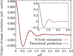
Figure 1: (Color on line) Comparison between $N$-body simulations and theoretical predictions given by (13) for small and large perturbations. Parameters are $\Delta t=0.001$, $N=10^{5}$, particles interaction $C=10^{-2}$, $l=1.0$, $\omega=17.8$, $\kappa_{0}=10.0$, $D=1.0$ and $\eta(0)\simeq 0.02\times L_{h}$. We use the same parameters for the inset except $\eta(0)\simeq 2\times L_{h}$.

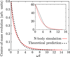
Figure 2: (Color on line) Comparison between $N$-body simulations and theoretical predictions given by (13) for small and large perturbations. Parameters are $\Delta t=0.001$, $N=10^{5}$, $C=1$, $l=1.0$, $\omega=17.8$, $\kappa_{0}=10.0$, $D=1.0$ and $\eta(0)\simeq 0.02\times L_{h}$. We use the same parameters for the inset except $\eta(0)\simeq 2\times L_{h}$.

Beyond the comparison between predictions and simulations, figures 1 and 2 show an interesting phenomenon: when the size of the system increases, the c.o.m. motion changes drastically. Small systems undergo an underdamped relaxation, whereas large systems become overdamped. Clearly, this is related to the ratio between the number of particles experiencing a large friction and those feeling a small friction. Eq. (9) yields an approximate value for the threshold. Indeed by considering the linear expansion of Eq. (9) we obtain the simple criterion:

$$\left\langle\frac{\partial\kappa(\mathbf{r},\mathbf{v})v_{j}}{\partial v_{j}}\right\rangle_{f_{0}}^{2}-4\left\langle\frac{\partial^{2}\Phi}{\partial r_{j}^{2}}(\mathbf{r})\right\rangle_{f_{0}}^{2}\left\{\begin{array}[]{ll}<0&\Rightarrow\text{Underdamped}\\ >0&\Rightarrow\text{Overdamped}\end{array}\right..$$ (14)

It leads to the critical number of particles (or equivalently interaction strength in our specific example, see Eq. (11)):

$$N_{c}=2\frac{l\omega^{2}}{C}\left(2\frac{\omega}{\kappa}-1\right),$$ (15)

and we conclude that for the same range of parameters, the behavior of c.o.m. of the plasma qualitatively changes when the number of particles increases.

III.2 Velocity dependent friction

We consider now another test case, where the friction varies linearly with the velocity:

$$\kappa(x,v)=\kappa(v)=\kappa_{0}\frac{|v|}{v_{0}},$$ (16)

with $v_{0}$ a typical velocity and $\kappa_{0}$ a typical friction.

We have no analytical expression for the stationary distribution $f_{0}$. However, we will see that a numerical estimation of $f_{0}$ is sufficient to obtain a quite good prediction of the c.o.m. motion. In this case, we consider the discrete distribution of particles $f_{0}^{N}$ obtain from numerical simulation, which is more or less the one particle distribution:

$$f_{0}^{N}(x,v)=\sum_{i=1}^{N}\delta(x-x_{i})\delta(v-v_{i})\simeq f_{0}(x,v).$$ (17)

Using $f_{0}^{N}$ to approximate $f_{0}$, Eq. (9) leads to

$$\ddot{\eta}+\omega^{2}\eta+\frac{\kappa_{0}}{N}\sum_{i=1}^{N}|v_{i}+\dot{\eta}|(v_{i}+\dot{\eta})=0.$$ (18)

The evolution of Eq. (18) is computed using a fourth-order Runge-Kutta method and figure 3 shows some simulations using (16) for different perturbation and diffusion coefficients. Agreement is not perfect but very good results are obtained for large perturbations. This shows that the dynamical ansatz method is not limited to small perturbations.

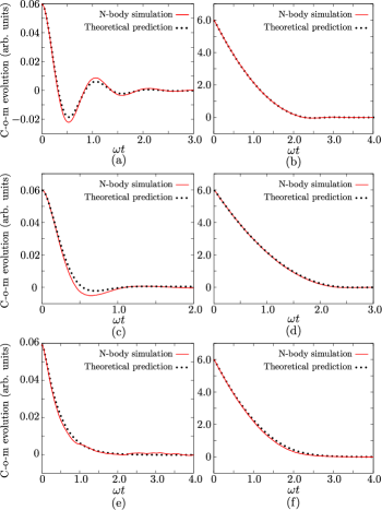
Figure 3: (Color on line) Comparison between $N$-body simulations (straight line) and theoretical predictions (dotted line) given by (18). Figures (a), (c), (e) corresponds to small perturbation $\eta(0)\simeq 0.02\times L_{h}$. Figures (b), (d), (f) corresponds to large perturbation $\eta(0)\simeq 2\times L_{h}$. The diffusion coefficient increases from top to bottom. (a)(b): $D=5$; (c)(d): $D=50$; (e)(f): $D=500$. Other parameters are $\Delta t=0.001$, $N=10^{5}$, $C=10^{-2}$, $v_{0}=1.0$, $\omega=17.8$ and $\kappa_{0}=10.0$. We continue to use parameter the $L_{h}$ because for these set of parameters the hypothesis of a strongly interacting or cold plasma is well satisfied.

In a similar manner as for the space-dependent friction case, we observe interesting features in figure 3. Varying the diffusion may change the dynamics of the c.o.m. This phenomenon can be understood as follows: when $D$ increases, particles explore a larger region in phase space, including parts with larger velocity. Considering Eq. (16), the particles are then more damped and the global evolution changes from underdamped to overdamped. Such a switching behavior between two qualitatively different evolutions has already been studied in different models with velocity dependent friction Mikhailov_1999 ; Erdmann_2005 ; Ebeling_2008 . In these papers the authors do not consider the c.o.m. motion, and in their cases the value of the diffusion coefficient implies a transition between a translation and a rotation mode. Nevertheless, we point out that the dynamical features are closely related to the nature of the friction and the shape of the one-particle distribution which depends on the diffusion coefficient $D$.

We now investigate a friction profile presenting large variations and a negative part:

$$\kappa(x,v)=\kappa(v)=-\kappa_{0}\left[1-\left(\frac{v}{v_{0}}\right)^{2}\right],$$ (19)

with $v_{0}$ a typical velocity and $\kappa_{0}$ the friction value at $v=0$. This friction profile is negative for $|v|<v_{0}$ and particles increase their energy in this region. With such a friction profile, the hypothesis underlying (6) are expected to be completely violated.

Figure 4 shows the comparison between direct numerical simulations, and the prediction using (9) with the discrete density $f_{0}^{N}$.

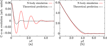
Figure 4: (Color on line) Comparison between $N$-body simulations (straight line) and theoretical predictions (dotted line) given by the friction profile (19). (a): $\eta(0)\simeq 0.02\times L_{h}$; (b): $\eta(0)\simeq 2\times L_{h}$. Other parameters are $\Delta t=0.001$, $N=10^{5}$, $C=10^{-2}$, $v_{0}=1.0$, $\omega=17.8$, $\kappa_{0}=10.0$ and $D=1.0$. We continue to use parameter $L_{h}$ because for these set of parameters the hypothesis of strongly/cold interacting plasma is well satisfied.

In this case, as could be anticipated, the dynamical ansatz fails to predict the c.o.m. motion. Indeed, a negative friction induces some local dilation/compression which are not included in the dynamical ansatz. For large perturbation we obtain a better result because the whole system starts in a positive friction region and the local dilation/compression effect become smaller. However, when the particles reach again negative friction a shift appears between prediction and simulation.

III.3 Anharmonic trap

In this section we consider a one dimensional plasma with constant friction $\kappa$ in an anharmonical trap. The trapping force used is:

$$\mathbf{F}_{trap}(x)=\frac{\omega^{2}}{1+4(\delta-\mu x)^{2}}-\frac{\omega^{2}}{1+4(\delta+\mu x)^{2}}$$ (20)

with $\boldsymbol{\nabla}_{x}\Phi(x)=-\mathbf{F}_{trap}(x)$, $\delta<0$ and $\mu>0$.

This kind of anharmonic trap appears for instance in some models of cold atoms in magneto-optical traps (see section IV).

Figure 5 shows a comparison between numerical simulation and prediction when the number of particles lying in the strongly anharmonic region becomes more and more important. To highlight this aspect, the figure represents the absolute trapping force $|F_{trap}(x)|$ and the linear trapping force obtained by expanding $F_{trap}(x)$ around $x=0$.

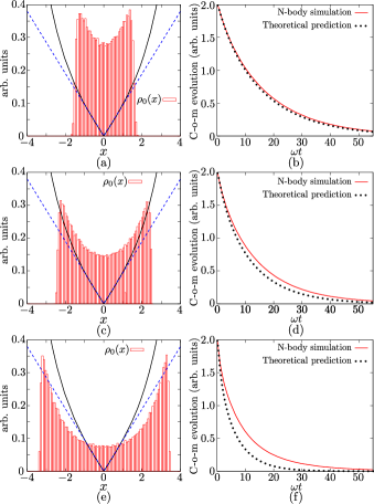
Figure 5: (Color on line) Figures (a), (c), (e): Space stationary state from $N$-body simulations and absolute trapping force $|F_{trap}(x)|$ (straight line). The absolute harmonic trapping force associated (dotted line) is included for reference purposes. Figures (b), (d), (f): Comparison between $N$-body simulations (straight line) and theoretical prediction (dotted line) given by the trapping force (20). The interaction strength increases from top to bottom: $C\in\{2.5,5,10\}(\times 10^{-5})$. Others parameters are $\Delta t=0.001$, $N=10^{5}$, $\eta(0)=2.0$, $\delta=-6.0$, $\mu=1.0$ $\omega=17.8$, $\kappa=10.0$ and $D=0.1$.

Clearly the dynamical ansatz fails to describe the whole c.o.m. dynamics when to number of particles in the anharmonic region becomes too important. We obtain the same results as for a negative velocity dependent friction: the dynamical ansatz hypothesis are not satisfied any more. As an example, Ott_2003 shows for a Bose-Einstein condensate that a non harmonic trap may lead to several new features. In their cases, they have identified several nonlinear effects due to anharmonicity, such as nonlinear mode mixing.

In conclusion, the dynamical ansatz method must be used with care when the number of particles in the anharmonic region is important in comparison with those in the harmonic one. On the other hand, the dynamical ansatz yields satisfactory results for the c.o.m. motion in a weakly anharmonic trap.

IV Application: Large Magneto-optical trap

Recently it has been shown that increasing the number of atoms in a magneto-optical traps (MOT) may trigger dynamical instabilities, that are absent in smaller clouds Pohl_2006 ; Labeyrie_2006 . In this section, we apply the previous results to the case of the magneto-optical trap. We start by briefly introducing one of the simplest ways to model a MOT with Rb⁸⁵ atoms using the transition $F=3\rightarrow F^{\prime}=4$ of the $D2$ line. We show that a the model naturally induces a space dependent friction, which leads to a qualitative change in the dynamics for the center-of-mass relaxation. Finally, we provide some experimental evidence confirming this prediction.

IV.1 Dynamics of the center-of-mass of a MOT

We use the so-called low-intensity Doppler model which is based on a velocity confinement due to the Doppler cooling and a spatial confinement due to the Zeeman effect Metcalf_1999 . Let us stress that we neglect the sub-Doppler effect. We assume that the contribution of the sub-Doppler cooling does not change qualitatively the behavior of a large MOT with Rubidium atoms. The average force $\mathbf{F}(\mathbf{r},\mathbf{v})$ acting on a single atom comes from the radiative pressure force:

$$\begin{array}[]{lcr}F^{i}(r_{i},v_{i})&=&\displaystyle\frac{\hbar k_{L}\Gamma}{2M}\frac{I_{0}}{I_{sat}}\frac{1}{1+\frac{4(\delta-\mu_{i}r_{i}-k_{L}v_{i})^{2}}{\Gamma^{2}}}\\ &-&\displaystyle\frac{\hbar k_{L}\Gamma}{2M}\frac{I_{0}}{I_{sat}}\frac{1}{1+\frac{4(\delta+\mu_{i}r_{i}+k_{L}v_{i})^{2}}{\Gamma^{2}}},\end{array}$$ (21)

with $F^{i}$ the $i^{th}$ component of F, $M$ the mass of Rb⁸⁵ atoms, $I_{0}$ the laser intensity of lasers beams along the six directions, $I_{sat}$ the saturation intensity, $\delta$ the detuning of the laser frequency $\omega_{L}$ with respect to the atomic resonance $\omega_{A}$ ($\delta=\omega_{L}-\omega_{A}<0$), $\Gamma$ the natural linewidth of the transition used, $k_{L}$ the laser wave number and $\mu_{i}r_{i}$ the Zeeman shift where $\mu_{i}$ depends on the applied magnetic field.

One usually considers the limit $k_{L}v_{i}/\delta\ll 1$ and $\mu_{i}r_{i}/\delta\ll 1$, which allows to extract a friction and a trapping force. In the case of a large low temperature MOT, we assume that linearization in space is less reasonable than a linearization velocity. The radiative pressure force becomes

$$\left\{\begin{array}[]{l}F^{i}(r_{i},v_{i})=F_{trap}^{i}(r_{i})-\kappa(r_{i})v_{i}+\mathcal{O}\left(v_{i}\right)\\ F_{trap}^{i}(r_{i})=\frac{\hbar k_{L}\Gamma}{2M}\frac{I_{0}}{I_{sat}}\left[\frac{\Gamma^{2}}{\Gamma^{2}+4(\delta-\mu_{i}r_{i})^{2}}-\frac{\Gamma^{2}}{\Gamma^{2}+4(\delta+\mu_{i}r_{i})^{2}}\right]\\ \kappa(r_{i})=-\frac{\hbar k_{L}\Gamma}{2M}\frac{I_{0}}{I_{sat}}\left[\frac{8k_{L}\Gamma^{2}(\delta-\mu_{i}r_{i})}{\left(\Gamma^{2}+4(\delta-\mu_{i}r_{i})^{2}\right)^{2}}+\frac{8k_{L}\Gamma^{2}(\delta+\mu_{i}r_{i})}{\left(\Gamma^{2}+4(\delta+\mu_{i}r_{i})^{2}\right)^{2}}\right].\end{array}\right.$$ (22)

In order to simplify our theoretical consideration and apply the dynamical ansatz method described in the section II, we consider the symmetric approximation of the friction part of Eq.(22) (in particular $\mu_{i}=\mu$):

$$\begin{array}[]{ll}\kappa(\mathbf{r})=&\displaystyle-\frac{\hbar k_{L}\Gamma}{2M}\frac{I_{0}}{I_{sat}}\times\\ &\displaystyle\left[\frac{8k_{L}\Gamma^{2}(\delta-\mu|\mathbf{r}|)}{\left(\Gamma^{2}+4(\delta-\mu|\mathbf{r}|)^{2}\right)^{2}}+\frac{8k_{L}\Gamma^{2}(\delta+\mu|\mathbf{r}|)}{\left(\Gamma^{2}+4(\delta+\mu|\mathbf{r}|)^{2}\right)^{2}}\right],\end{array}$$ (23)

which coincides with expression (22) along the axis. This approximate friction (23) should preserve the important features of the system, albeit in a simplified way.

It is commonly known in the cold-atoms community that this model is restricted to small MOT Sesko_1991 , i.e. small number of particles. For large MOT we have to consider two other contributions: an attractive force $\mathbf{F}_{A}$ which comes from a screening effect, and a repulsive force which comes from multiple scattering. In the small optical width region, these two forces satisfy Sesko_1991 :

$$\boldsymbol{\nabla}.\left[\mathbf{F}_{A}(\mathbf{r})\right]=-\frac{\sigma_{L}^{2}I_{0}}{c}\rho(\mathbf{r})$$ (24)

and

$$\boldsymbol{\nabla}.\left[\mathbf{F}_{R}(\mathbf{r})\right]=\frac{\sigma_{R}\sigma_{L}I_{0}}{c}\rho(\mathbf{r}),$$ (25)

where $\sigma_{L}$ (resp. $\sigma_{R}$) is the laser absorption (resp. atom scattering) cross section, $c$ the light velocity. Assuming that $\mathbf{F}_{A}$ and $\mathbf{F}_{R}$ derive from a potential (which is not true for the former), we can use the Gauss theorem to consider these forces as a Coulombian binary interaction force:

$$\mathbf{F}_{bin}(\mathbf{r},\mathbf{r}^{\prime})=C\times\frac{\mathbf{r}-\mathbf{r}^{\prime}}{|\mathbf{r}-\mathbf{r}^{\prime}|^{3}}.$$ (26)

The MOT is then described as a non-neutral plasma. When the temperature is low enough and the anharmonicity is weak, we obtain the same property as the toy-model used in our numerical test, i.e. a stationary state:

$$\rho_{0}(\mathbf{r})=\int f_{0}(\mathbf{r},\mathbf{v})d\mathbf{v}=\left\{\begin{array}[]{cl}\frac{3\omega^{2}}{C}&\text{, if }|\mathbf{r}|<L_{h}\\ 0&\text{, elsewhere}\end{array},\right.$$ (27)

with $L_{h}^{3}=NC/(4\pi\omega^{2})$.

Exactly as in section III.1, we show that the friction profile given in Eq. (23) leads to transitions between overdamped or underdamped relaxation when the number of particles change. To predict the transitions between these two behaviors we linearize equation Eq. (9). If we consider a perturbation along the $i^{th}$ direction, we obtain the condition:

$$\left\langle\kappa(\mathbf{r})\right\rangle_{f_{0}}^{2}-4\left\langle\frac{\partial^{2}\Phi}{\partial r_{i}^{2}}(\mathbf{r})\right\rangle_{f_{0}}\left\{\begin{array}[]{ll}<0&\Rightarrow\text{Underdamped}\\ >0&\Rightarrow\text{Overdamped}\end{array}\right.$$ (28)

We represent on figure 6 the different behaviors, depending on the detuning $\delta$ and the magnetic field $\nabla B$ when the size of the system increases i.e. when the number of particles increase. It is possible to obtain three different behaviors depending on the parameter values: underdamped relaxation; overdamped relaxation; or the stationary state is unstable. This latter possibility corresponds to $\langle\kappa(\mathbf{r})\rangle_{f_{0}}<0$. This implies that $\kappa(\mathbf{r})$ can be negative and that a lot of particles lies in those regions. We will not discuss this case anymore since our numerical tests show that the method is unreliable when negative friction plays a role. An important feature shown in figure 6 is that for the same value of detuning and magnetic field, it is possible to observe a modification of the relaxation dynamics by increasing the number of atoms.

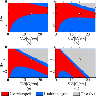
Figure 6: (Color on line) Theoretical behavior of the c.o.m. mode relaxation in the parameters plane ($\nabla B;\delta/\Gamma$) for different system sizes. The diamond shows the dynamical changes experienced by the c.o.m. motion as the MOT’s size increases, at fixed parameter values ($15;-1$). (a): $L_{h}=0.5$ mm; (b): $L_{h}=1$ mm; (c): $L_{h}=2$ mm; (d): $L_{h}=4$ mm. Other parameters are $k_{L}=2\pi/\lambda$ with $\lambda=780\times 10^{-9}$ m and $\mu=2\pi\mu_{0}g\nabla B$ with $\mu_{0}=2.1\times 10^{6}$ G^-1 and $g=1.0$ an effective Landé g-factor of the transition used.

For example, increasing $L_{h}$ from $0.5$ mm to $4$ mm with $\delta/\Gamma=-2.5$ and $\nabla B=15$ G/cm, the relaxation of the center-of-mass changes from underdamped to overdamped. Considering the friction profile obtained for those parameters (see figure 7) and using the same consideration as in section III, we are able to understand this behavior: $\left\langle\kappa(\mathbf{r})\right\rangle_{f_{0}}$ is just the average friction felt by the whole system; the threshold separating overdamped and underdamped is obtained by comparing this average friction with $\left\langle\partial^{2}\Phi/\partial r_{i}^{2}(\mathbf{r})\right\rangle_{f_{0}}$. Figure 7 represent these quantities for harmonic trap to simplify as much as possible the discussion. When the size of the system is roughly between $2.5-3$ mm, the local friction at the edge of the system is higher than the critical friction, nevertheless the system is underdamped because the average friction stays below the threshold. For $|\mathbf{r}|\geq 3$ mm the system becomes overdamped. For an even larger cloud, the friction decreases, the system may become underdamped again (not seen in the figure).

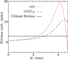
Figure 7: (Color on line) Representation of the different friction depending on the size of the system for $\delta/\Gamma=-2.5$ and $\nabla B=15$ G/cm. Dotted line: friction profile $\kappa(\mathbf{r})$ given by (23); dashed line: average friction $\langle\kappa(\mathbf{r})\rangle_{f_{0}}$; straight line: critical friction considering the harmonic approximation of the trapping potential $\Phi$.

Let us stress that we used a simple model based on Doppler cooling to describe a MOT and many phenomena are not included in our study: sub-Doppler cooling is neglected (this can be important for the c.o.m. relaxation in small systems); the friction profile is assumed to be independent on the number of particles; the “effective charge” in the interaction force is taken as a constant. We do not expect this model to predict exactly the transition between the different regimes; however, in some cases the Doppler model should be sufficient to describe qualitatively the system. Note that Xu_2002 shows that atomic properties may dramatically changes the relaxation: for alkaline-earth-metal atoms it is possible to observe underdamped oscillations Xu_2002 , while the same regime with alkali-metal atoms shows a strongly overdamped relaxation Steane_1991 .

IV.2 Experimental results

We present here some experimental evidence supporting the analysis developed in the previous section. Our experimental setup has been described elsewhere Labeyrie_2006 . We load a large magneto-optical trap containing up to 2$\times 10^{10}$ Rb⁸⁵ atoms from a dilute room-temperature vapor. The MOT employs 6 large (waist = 4 cm) independent laser beams, tuned slightly below (typically by $-3\Gamma$) the $F=3\rightarrow F^{\prime}=4$ transition of the $D2$ line. An additional repumping beam is also applied to the atoms, whose intensity is used to control the number of atoms in the $F=3$ hyperfine level. To study the dynamics of the MOT’s center-of-mass, we image the fluorescence light of the cloud on a photodiode, with a mask blocking half of the MOT’s image (see figure 8(a)). This setup is thus sensitive to any displacement of the center-of-mass of the cloud in the plane orthogonal to the line of sight of the imaging optics.

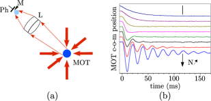
Figure 8: (Color on line) Experimental observation of number-dependent MOT center-of-mass dynamics. (a) Detection setup. A fluorescence image of the MOT is formed on a photodiode (Ph) using lens (L). A mask (M) blocks half of the MOT image, rendering the photodiode signal sensitive to a lateral displacement of the MOT. (b) N-dependent dynamics. We record the sloshing motion of the cloud following a small displacement of the trap at $t=0$. The different curves correspond to an increasing number of atoms from top to bottom.

Figure 8(b) shows the measured impact of the atom number on the dynamics of the MOT’s center-of-mass. Using an offset magnetic field, we displace the MOT’s center-of-mass. When this offset field is switched off at $t=0$, the MOT is free to evolve in the initial trapping conditions and the MOT then returns to its equilibrium position. As shown on figure 8(b), for low atom number the dynamics of the center of mass is overdamped, typical for standard MOTs. However we observe a clear transition from an overdamped behavior at low atom number, to an underdamped one when the atom number is large. This cross-over is heralding the instability regime observed in Labeyrie_2006 . This transition to an underdamped motion of the center of mass of the MOT before reaching the instability regime is similar to the narrow region indicated in blue in figure 6 separating the overdamped region from the instability region.

V Conclusion

In the present work we have introduced a dynamical ansatz to obtain an approximate evolution of the center-of-mass mode considering a trapped system of interacting particles, assuming a global translation of the whole system. This approach allows to describe numerous problems with arbitrary perturbation amplitudes of the center-of-mass mode. This includes systems with space and/or velocity dependent friction as well as anharmonic trapping potential. We have confronted the predictions of the simplified approach with direct $N$-body simulations of Langevin equations, considering a one dimensional plasma with different friction and trap profiles as test case. The main conclusion is that the agreement is satisfactory as long as the hypotheses underlying the ansatz are well enough satisfied. Using this approach on a model for a magneto-optical trap, we predict transitions between overdamped and underdamped motion for the center of mass of the cloud, as the number of trapped atoms increases. Finally, we provide some experimental evidence for such a transition, thus confirming some of the predictions made.

Note that we assume in this work a constant diffusion coefficient and an external force which derives from a potential. However it is straightforward to extend the dynamical ansatz method. For instance in the case of a space and/or velocity dependent diffusion or with rotational forces. Finally a combination of the dynamical ansatz introduced in this paper and the scaling ansatz method detailed in Olivetti_2009 ; Olivetti_2011 may be useful to describe simultaneously the center-of-mass motion and the breathing mode oscillation Guery_Odelin_2002 .

- (1) W. Kohn, Phys. Rev. 123, 1242 (1961).
- (2) M. Bonitz, C. Henning, and D. Block, Rep. Prog. Phys. 73, 066501 (2010).
- (3) A. Melzer, M. Klindworth, and A. Piel, Phys. Rev. Lett. 87, 115002 (2001).
- (4) T.E. Sheridan, Phys. Rev. E 72, 026405 (2005).
- (5) H. Moritz, T. Stoferle, M. Kohl, and T. Esslinger, Phys. Rev. Lett. 91, 250402 (2003).
- (6) M. Bonitz, K. Balzer, and R. van Leeuwen, Phys. Rev. B 76, 045341 (2007).
- (7) C. Henning, K. Fujioka, P. Ludwig, A. Piel, A. Melzer, and M. Bonitz, Phys. Rev. Lett. 101, 045002 (2008).
- (8) S.A. Trigger and A.G. Zagorodny, Contrib. Plasma Phys. 43, 381 (2003).
- (9) S.A. Trigger, W. Ebeling, A.M. Ignatov and I.M. Tkachenko, Contrib. Plasma Phys. 43, 377 (2003).
- (10) J. Dunkel, W. Ebeling, and S.A. Trigger, Phys. Rev. E 70, 046406 (2004).
- (11) A.S. Mikhailov, and D.H. Zanette, Phys. Rev. E 60, 4571 (1999).
- (12) U. Erdmann, W. Ebeling, and A.S. Mikhailov, Phys. Rev. E 71, 051904 (2005).
- (13) W. Ebeling and L. Schimansky-Geier, Eur. Phys. J. Special Topics 157, 17 (2008).
- (14) G. Labeyrie, F. Michaud, and R. Kaiser, Phys. Rev. Lett. 96, 023003 (2006).
- (15) T. Pohl, G. Labeyrie, and R. Kaiser, Phys. Rev. A 74, 023409 (2006).
- (16) H. Ott, J. Fortagh, S. Kraft, A. Gunther, D. Komma, and C. Zimmermann, Phys. Rev. Lett. 91, 040402 (2003).
- (17) D. Talay, Tech. Report INRIA, 1313 (1990).
- (18) J. Barnes, P. Hut, Nature 324, 446 (1986).
- (19) A. Olivetti, J. Barré, B. Marcos, F. Bouchet, and R. Kaiser, Transport Theory and Statistical Physics, 39, 524 (2010).
- (20) H.J. Metcalf, and P. Straten, Laser Cooling and Trapping Springer-Verlag, New York (1999).
- (21) D.W. Sesko, T.G. Walker, and C.E. Wiemann, J. Opt. Soc. Am. B 8, 946 (1991).
- (22) X. Xu, T.H. Loftus, M.J. Smith, J.L. Hall, A. Gallagher and J. Ye, Phys. Rev. A 66 011401(R) (2002).
- (23) A.M. Steane and C.J. Foot, Europhys. Lett. 14 231 (1991).
- (24) A. Olivetti, J. Barré, B. Marcos, F. Bouchet, and R. Kaiser, Phys. Rev. Lett. 103, 224301 (2009).
- (25) D. Guéry-Odelin (2002), Phys. Rev. A 66, 033613 (2002).