Experimental Passive Decoy-State Quantum Key Distribution

Abstract

The decoy-state method is widely used in practical quantum key distribution systems to replace ideal single photon sources with realistic light sources by varying intensities. Instead of active modulation, the passive decoy-state method employs built-in decoy states in a parametric down-conversion photon source, which can decrease the side channel information leakage in decoy state preparation and hence increase the security. By employing low dark count up-conversion single photon detectors, we have experimentally demonstrated the passive decoy-state method over a 50-km-long optical fiber and have obtained a key rate of about 100 bit/s. Our result suggests that the passive decoy-state source is a practical candidate for future quantum communication implementation.

1 Introduction

Quantum key distribution (QKD) [1, 2] can provide unconditionally secure communication with ideal devices [3, 4, 5]. In reality, due to the technical difficulty of building up ideal single photon sources, most of current QKD experiments use weak coherent-state pulses from attenuated lasers. Such replacement opens up security loopholes that lead QKD systems to be vulnerable to quantum hacking, such as photon-number-splitting attacks [6]. The decoy-state method [7, 8, 9, 10, 11] has been proposed to close these photon source loopholes. It has been implemented in both optical fiber [12, 13, 14, 15, 16, 17] and free space channels [18, 19].

The security of decoy-state QKD relies on the assumption of the photon-number channel model [11, 20, 21], where the photon source can be regarded as a mixture of Fock (number) states. In practice, this assumption can be guaranteed when the signal and decoy states are indistinguishable to the adversary party, Eve, other than the photon-number information.

Otherwise, if Eve is able to distinguish between signal and decoy states via other degrees of freedom, such as frequency and timing of the pulses, the security of the decoy-state protocol would fail [13, 22]. In the original proposals, on the transmitter’s side, Alice actively modulates the intensities of pulses to prepare decoy states through an optical intensity modulator, as shown in Fig. 1 (a). This active decoy-state method, however, might leak the signal/decoy information to Eve due to intensity modulation and increase the complexity of the system.

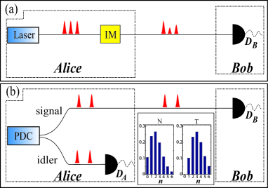
Figure 1: (a) In the active decoy-state method, Alice employs an intensity modulator (IM) to vary the average photon numbers of the attenuated weak coherent pulses. (b) In the passive decoy-state method, Alice infers the two different photon number distributions of the signal mode from the detection results of the idler mode, $N$ (non-triggered) and $T$ (triggered), respectively. The inset shows the photon number distributions conditioned on the detection results of the idler mode.

Another type of protocols, passive decoy-state method, has been proposed, where the decoy states are prepared through measurements [23, 24, 25]. The passive method can rely on the usage of a parametric down-conversion (PDC) source where the photon numbers of two output modes are strongly correlated. As shown in Fig. 1 (b), Alice first generates photon pairs through a PDC process and then detects the idler photons as triggers. Conditioned on Alice’s detection outcome of the idler mode, trigger ($T$) or non-trigger ($N$), Alice can infer the corresponding photon number statistics of the signal mode, and hence obtains two conditional states for the decoy-state method. The photon numbers of these two states follow different distributions as shown in Appendix. From this point of view, the PDC source can be treated as a built-in decoy state source. Note that passive decoy-state sources with Non-Poissonian light other than PDC sources are studied in [26, 27, 28, 29, 30, 31]. Also, the PDC source can be used as a heralded single photon source in the active decoy-state method [32].

The key advantage of the passive decoy-state method is that it can substantially reduce the possibility of signal/decoy information leakage [25, 33]. In addition, the phases of signal photons are totally random due to the spontaneous feature of the PDC process. This intrinsic phase randomization improves the security of the QKD system [34], by making it immune to source attacks [35, 36]. The critical experimental challenge to implement passive decoy-state QKD is that the error rate for the non-trigger case is very high due to high vacuum ration and background counts. Besides, as a local detection, the idler photons do not suffer from the modulation loss and channel loss, so the counting rate of Alice’s detector is very high. Due to the high dark count rate and low maximum counting rate, commercial InGaAs/InP avalanche photodiodes (APD) are not suitable for these passive decoy-state QKD experiments. By developing up-conversion single photon detectors with high efficiency and low noise, we are able to suppress the error rate in the non-trigger events. Meanwhile, the up-conversion single photon detectors can reach a maximum counting rate of about 20 MHz. With such detectors, we demonstrates the passive decoy-state method over a 50-km-long optical fiber.

2 Photon number distribution of the PDC source

For the decoy-state method, the photon number distribution of the source is crucial for data postprocessing [37, 25]. Thus, we first investigate the photon number distribution of the PDC source used in the experiment, as shown in Fig. 2 (a). An electronically driven distributed feedback laser triggered by an arbitrary function generator is used to provide a 100 MHz pump pulse train. After being amplified by an erbium-doped fiber amplifier (EDFA), the laser pulses with a 1.4 ns FWHM duration and 1556.16 nm central wavelength pass through a 3 nm tunable bandpass filter to suppress the amplified spontaneous emission noise from the EDFA. The light is then frequency doubled in a periodically poled Lithium Niobate (PPLN) waveguide. Since our waveguide only accepts TM-polarized light, an in-line fiber polarization controller is used to adjust the polarization of the input light. The generated second harmonic pulses are separated from the pump light by a short-pass filter with an extinction ratio of about 180 dB, and then used to pump the second PPLN waveguide to generate correlated photon pairs. Both PPLN waveguides are fiber pigtailed reverse-proton-exchange devices and each has a total loss of 5 dB. The generated photon pairs are separated from the pump light of the second PPLN waveguide by a long-pass filter with an extinction ratio of about 180 dB. The down converted signal and idler photons are separated by a 100 GHz dense wavelength-division multiplexing (DWDM) fiber filter. The central wavelengths of the two output channels of the DWDM filter are 1553.36 nm and 1558.96 nm.

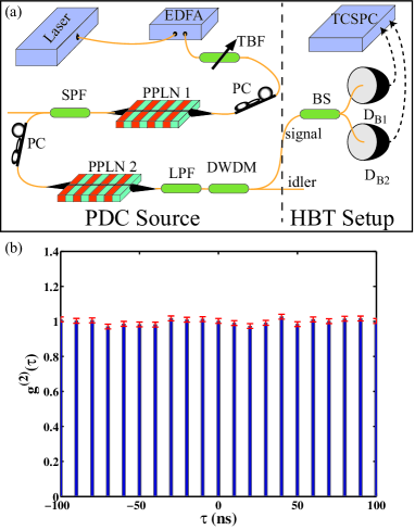
Figure 2: (a) A schematic diagram of the PDC source test. EDFA: erbium-doped fiber amplifier; TBF: tunable bandpass filter; PPLN: periodically poled Lithium Niobate; PC: polarization controller; SPF: short-pass filter; LPF: long-pass filter; DWDM: dense wavelength-division multiplexing; BS: 50:50 beam splitter; TCSPC: time correlated single photon counting. (b) Normalized second-order correlation function of the photons in the signal mode. The parameter $\tau$ represents the time delay between the photons of the two BS output arms. The value of $g^{(2)}(0)$ is $0.994\pm 0.014$.

For a spontaneous PDC process, the number of emitted photon pairs within a wave package follows a thermal distribution [38]. In the case when the system pulse length is longer than the wave package length, the distribution can be calculated by taking the integral of thermal distributions. In the limit when the pulse length is much longer than the wave package length, the integrated distribution can be well estimated by a Poisson distribution [39, 40]. In our experiment, the pump pulse length is 1.4 ns, while the length of the down-conversion photon pair wave package is around 4 ps. Therefore, the photon pair number statistics can be approximated by a Poisson distribution. To verify this, we build a Hanbury Brown-Twiss (HBT) setup [41] by inserting a 50:50 beam splitter (BS) in the signal mode followed by two single photon detectors, as shown in Fig. 2 (a). Both detection signals are feeded to a time correlated single photon counting (TCSPC) module for time correlation measurement. A time window of 2 ns is used to select the counts within the pulse duration. The interval between the peaks of counts is 10 ns, which is consistent with the 100 MHz repetition rate of our source. After accumulating about 5000 counts per time bin, we calculate the value of the normalized second-order correlation function $g^{(2)}(\tau)$ of the signal photons, which is shown in Fig. 2 (b). The value of $g^{(2)}(0)$ is $0.994\pm 0.014$, which confirms the Poisson distribution of the photon pair number.

3 Experimental setup and key rate

Our passive decoy-state QKD experimental setup is shown in Fig. 3. The PDC source is placed on Alice’s side. The idler photons are detected by an up-conversion single photon detector whose outcomes are recorded by a field programable gate array (FPGA) based data acquisition card and then transmitted to a computer. The up-conversion single photon detector used in our experiment consists of a frequency up-conversion stage in a nonlinear crystal followed by detection using a silicon APD (SAPD). As described in [42], a 1950 nm Thulium doped fiber laser is employed as a pump light for a PPLN waveguide, which is used to up-convert the wavelength of the idler photons to 866 nm. After filtering the pump and other noise in the up-conversion process, we detect the output photons with a SAPD. By using the long-wavelength pump technology, we can suppress the noise to a very low level and achieve a detection efficiency of 15% and a dark count rate of 800 Hz.

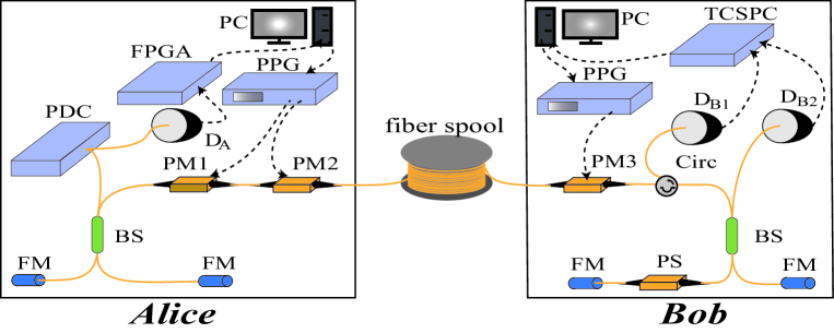
Figure 3: The schematic diagram of our experimental setup. BS: 50:50 beam splitter; FM: Faraday mirror; PM: phase modulator; FPGA: field programmable gate array; PPG: pulse pattern generator; Circ: optical circulator; PS: phase shifter. The detectors used in the experiment are up-conversion single photon detectors.

For signal photons, we employ the phase-encoding scheme by using an unbalanced Faraday-Michelson interferometer and two phase modulators (PM), as shown in Fig. 3. The time difference between two bins is about 3.7 ns. The two PMs are driven by a 3.3 GHz pulse pattern generator (PPG). The first PM is utilized to choose the $X$ or $Y$ basis by modulating the relative phase of the two time bins into $\{0,\frac{1}{2}\pi\}$, respectively. The second PM is utilized to choose the bit value by modulating the relative phase into $\{0,\pi\}$. The encoded photons are transmitted to the receiver (Bob) through optical fiber. Bob chooses basis with a PM driven by another PPG and measures the relative phase of two time bins via an unbalanced interferometer with the same time difference of 3.7 ns. The random numbers used in the experiment are generated by a quantum random number generator (IDQ Quantis-OEM) beforehand and stored on the memory of the PPGs. The detection efficiency and dark count rate of the up-conversion detectors on Bob’s side are 14% and 800 Hz, respectively. Note that although the PM for encoding may also induces side channel leakage [22], the intent of this letter is to close the loophole due to the decoy state preparation, not to close all the loopholes in one experiment. And furthermore, we remark that BB84 qubit encoding can also be done via passive means [43]. Such step can be taken in future works.

One challenge in the experimental setup is to stabilize the relative phase of two unbalanced arms in two separated unbalanced interferometers, which is very sensitive to temperature or mechanical vibration. We place a piezo-electric phase shifter in one arm of the interferometer on Bob’s side for active phase feedback. After every second of QKD, Alice sends time-bin qubits without encoding and Bob records the detection results without choosing basis. The detection results are used for feedback to control the piezo-electric phase shifter.

After quantum transmission, Alice tells Bob the basis and trigger ($T$ or $N$) information. Bob groups his detection events accordingly and evaluates the gain $Q_{j}$ and QBER $E_{j}$, where $j=T,N$. They can distill secret key from both $N$ and $T$ events. Thus, the total key generation rate is given by

$$R=R_{N}+R_{T},$$ (1)

where $R_{N}$, $R_{T}$ are key rates distilled from $N$ and $T$ events, respectively. Following the security analysis of the passive decoy state scheme [25], the secret key rate is given by

$$R_{j}\geq q\{-fQ_{j}H(E_{j})+Q_{j,1}[1-H(e_{1})]+Q_{j,0}\},$$ (2)

where $j=N,T$; $q$ is the raw data sift factor (in the standard BB84 protocol $q=1/2$); $f$ is the error correction inefficiency (instead of implementing error correction, we estimate the key rate by taking $f=1.2$ , which can be realized by the low-density parity-check code[44]); $Q_{j}$ and $E_{j}$ are the gain and QBER; $Q_{j,1}$ and $e_{1}$ are the gain and error rate of the single-photon component; $Q_{j,0}$ is the background count rate; $H(x)=-x\mathrm{log}_{2}(x)-(1-x)\mathrm{log}_{2}(1-x)$ is the binary Shannon entropy function. Alice and Bob can get the gains and QBERs, $Q_{N}$, $Q_{T}$, $E_{N}$, $E_{T}$, directly from the experiment result. The variables for privacy amplification part, $Q_{j,1}$, $e_{1}$, and $Q_{j,0}$, need to be estimated by the decoy state method. Details of decoy state estimation as well as the method of postprocessing and simulation used later can be found in Appendix.

We perform the passive decoy-state QKD over optical fibers of 0 km, 25 km and 50 km. For each distance, we run the system for 20 minutes, half of which is used for phase feedback control. Thus the effective QKD time is 10 minutes and the system repetition rate is 100 MHz. Therefore, the number of pulses sent by Alice for each distance is N=60 Gbit. We analyze the time correlation of the detection results and calibrate the average photon number generated in the PDC source, $\mu_{0}$, using the measurement value of the coincidence to accidental coincidence ratio (CAR) [45]. The average photon number Alice sends to the channel, $\mu$, can be calculated as $\mu=\eta_{s}\mu_{0}$, where $\eta_{s}$=19.2 dB is the loss including the transmission loss of the PDC source and the modulation loss of Alice. The experimental results are listed in Table 1. After the postprocessing, we obtain a final key of 2.53 Mbit, 805 kbit, and 89.8 kbit for 0 km, 25 km, and 50 km, respectively.

Table 1: Experimental results. The number of pulses sent by Alice in each case is $N=6\times 10^{10}$. $N_{A}$ is the total number of photons detected by Alice. $\eta$ represents the transmittance taking channel loss, the modulation loss and detection efficiency on Bob’s side into account.

• Parameter	0 km	25 km	50 km
  $\mu$	0.035	0.036	0.028
  $N_{A}$	$4.22\times 10^{9}$	$4.14\times 10^{9}$	$3.99\times 10^{9}$
  $\eta$	21.8 dB	25.2 dB	30.4 dB
  $Q_{T}$	$2.21\times 10^{-5}$	$1.02\times 10^{-5}$	$2.50\times 10^{-6}$
  $Q_{N}$	$2.13\times 10^{-4}$	$1.02\times 10^{-4}$	$2.43\times 10^{-5}$
  $E_{T}$	$1.97\%$	$2.81\%$	$3.06\%$
  $E_{N}$	$2.12\%$	$3.15\%$	$3.99\%$

To compare the experimental results of key rate with QKD simulation, we set the values of simulation parameters, $\mu$, $N_{A}$ and $\eta_{s}$, to parameters used in the 50 km QKD experiment. We also calibrate our system to obtain a few parameters for simulation: $e_{d}=1.2\%$ – the error rate of Bob’s detector; and $Y_{0}=1.6\times 10^{-6}$ – background count rate of Bob’s detection. The comparison is shown in Fig. 4. As one can see that the experimental results are consistent with the simulation results. Note that there is an inflection point at about 31.7 dB, where $R_{N}$ drops to 0 and $R_{T}$ is still positive.

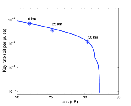
Figure 4: Comparison of theoretical values and experimental results of key rate. The loss consists of the loss of channel and the modulation loss and detection efficiency on Bob’s side. The solid line represents the simulation values of key rate. The stars are the experimental results.

4 Conclusions

We investigate a parametric down-conversion photon source pumped by a pulse laser for the usage in passive decoy-state QKD. The experimental result suggests that the photon-pair number of the PDC source can be well approximated by a Poisson distribution. With this source, we have experimentally demonstrated a passive decoy-state QKD scheme.

In our experiment, the transmission loss of the PDC source is about 7 dB, the total modulation loss caused by the two UFMIs and the three PMs is about 21 dB. These losses result in a significantly reduced key rate. However, there is room for improvement: if new-type MZIs [16] are used, the modulation loss of our system can be reduced by 9 dB; we can have a reduction of about 3 dB in loss if a state-of-the-art PPLN waveguide is used. Aiming for long distance QKD, we can also improve the up-conversion single photon detector by using a volume Bragg grating as a filter, and achieve a detection efficiency of about 30% with dark count rate less than 100 Hz [42]. In addition, the repetition rate of our system can be raised to 10 GHz [45]. These feasible improvements mean it is potential to perform passive decoy-state QKD over 150 km in optical fibers. Beside the PDC based scheme used in our experiment, there are other practical scenarios of passive decoy-state QKD, for example, those based on thermal states or phase randomized coherent states [26, 27, 28]. However, the physics and applications of these protocols demand further theoretical and experimental studies.

Appendix A method of postprocessing and simulation

The model of our passive decoy-state QKD experiment setup is shown in Fig. 5. $\mu_{0}$ denotes the average photon pair number of the PDC source. $\eta_{s}$ denotes Alice’s internal transmittance including the transmission loss of the PDC source and Alice’s modulation loss. $\mu$ denotes the average photon number of the signals sent to Bob, thus

$$\mu=\eta_{s}\mu_{0}.$$ (3)

$\eta_{A}$ denotes the transmittance of the idler mode taking into account transmission loss of the source and the detection efficiency. $\eta$ denotes the transmittance taking channel loss, the modulation loss and detection efficiency on Bob’s side into account. All the parameters can be characterized by Alice before the experiment except for $\eta$ which could be controlled by Eve.

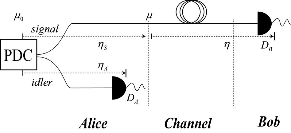
Figure 5: Model of the passive decoy-state QKD experimental setup.

Since Alice uses threshold detectors, the probabilities that Alice’s detector does not click ($N$) and clicks ($T$) when $i$ photons arrive are

$$P_{N|i}=(1-Y_{0A})(1-\eta_{A})^{i}\simeq(1-\eta_{A})^{i},$$ (4)

$$P_{T|i}=1-P_{N|i},$$ (5)

where $Y_{0A}$ denotes the dark count rate of Alice’s detection and it is about the order of $10^{-6}$ so that we just ignore it.

The joint probabilities that Alice has $N/T$ detection and $i$ photons are sent to Bob are given by

$$P_{N}(i) =\sum\limits_{j=i}^{\infty}\frac{(\mu_{0})^{j}}{j!}e^{-\mu_{0}}(1-\eta_{A})^{j}\left({\begin{array}[]{*{20}{c}}j\\ i\\ \end{array}}\right)\eta_{s}^{i}(1-\eta_{s})^{j-i}$$ (8)

$$=\frac{\mu^{i}}{i!}e^{-\mu}(1-\eta_{A})^{i}e^{-(\mu_{0}-\mu)\eta_{A}},$$ (9)

$$P_{T}(i) =\sum\limits_{j=i}^{\infty}\frac{(\mu_{0})^{j}}{j!}e^{-\mu_{0}}[1-(1-\eta_{A})^{j}]\left({\begin{array}[]{*{20}{c}}j\\ i\\ \end{array}}\right)\eta_{s}^{i}(1-\eta_{s})^{j-i}$$ (12)

$$=\frac{(\mu)^{i}}{i!}e^{-\mu}[1-(1-\eta_{A})^{i}e^{-(\mu_{0}-\mu)\eta_{A}}].$$ (13)

Define the yield $Y_{i}$ as the conditional probability that Bob gets a detection given that Alice sends $i$ photons into the channel and $e_{i}$ as the corresponding error rate. Then the gains that Alice has an $N/T$ detection and Bob has an $i$-photon detection are given by

$$Q_{N,i}=P_{N}(i)Y_{i}=\frac{\mu^{i}}{i!}e^{-\mu}(1-\eta_{A})^{i}e^{-(\mu_{0}-\mu)\eta_{A}}Y_{i},$$ (14)

$$Q_{T,i}=P_{T}(i)Y_{i}=\frac{(\mu)^{i}}{i!}e^{-\mu}[1-(1-\eta_{A})^{i}e^{-(\mu_{0}-\mu)\eta_{A}}]Y_{i}.$$ (15)

Thus, the overall gains when Alice gets an $N/T$ detection are

$$Q_{N}=\sum\limits_{i=0}^{\infty}Q_{N,i}=\sum\limits_{i=0}^{\infty}\frac{(\mu)^{i}}{i!}e^{-\mu}(1-\eta_{A})^{i}e^{-(\mu_{0}-\mu)\eta_{A}}Y_{i},$$ (16)

$$Q_{T}=\sum\limits_{i=0}^{\infty}Q_{T,i}=\sum\limits_{i=0}^{\infty}\frac{(\mu)^{i}}{i!}e^{-\mu}[1-(1-\eta_{A})^{i}e^{-(\mu_{0}-\mu)\eta_{A}}]Y_{i}.$$ (17)

The corresponding quantum bit error rates (QBERs) are given by

$$E_{N}Q_{N} =\sum\limits_{i=0}^{\infty}e_{i}Q_{N,i}$$ (18)

$$=\sum\limits_{i=0}^{\infty}\frac{\mu^{i}}{i!}e^{-\mu}(1-\eta_{A})^{i}e^{-(\mu_{0}-\mu)\eta_{A}}e_{i}Y_{i},$$ (19)

$$E_{T}Q_{T} =\sum\limits_{i=0}^{\infty}e_{i}Q_{T,i}$$ (20)

$$=\sum\limits_{i0}^{\infty}\frac{\mu^{i}}{i!}e^{-\mu}[1-(1-\eta_{A})^{i}e^{-(\mu_{0}-\mu)\eta_{A}}]e_{i}Y_{i}.$$ (21)

For simulation purpose, we consider the case that Eve does not change $Y_{i}$ and $e_{i}$. They are given by

$$Y_{i}=1-(1-Y_{0})(1-\eta)^{i},$$ (22)

$$e_{i}Y_{i}=e_{d}Y_{i}+(e_{0}-e_{d})Y_{0},$$ (23)

where $Y_{0}$ is the dark count rate of Bob’s detection, $e_{0}=1/2$ is the error rate of the dark count, and $e_{d}$ is the intrinsic error rate of Bob’s detection.

The gains of single-photon and vacuum states are given by

$${Q_{N,1}}=\mu{{\rm{e}}^{-\mu}}(1-{\eta_{A}})e^{-(\mu_{0}-\mu)\eta_{A}}{Y_{1}},$$ (24)

$${Q_{T,1}}=\mu{{\rm{e}}^{-\mu}}[1-(1-{\eta_{A}})e^{-(\mu_{0}-\mu)\eta_{A}}]{Y_{1}},$$ (25)

$${Q_{N,0}}={\rm{e}}^{-[\mu+(\mu_{0}-\mu)\eta_{A}]}{Y_{0}},$$ (26)

$${Q_{T,0}}={{\rm{e}}^{-\mu}}[1-e^{-(\mu_{0}-\mu)\eta_{A}}]{Y_{0}}.$$ (27)

Note that, for postprocessing, the values of $Q_{N}$, $Q_{T}$, $E_{N}$, $E_{T}$ should be obtained directly from the experiment. The overall gains when Alice gets an $N/T$ detection are given by

$$Q_{N}=e^{-\mu_{0}\eta_{A}}[1-(1-Y_{0})e^{\mu\eta(\eta_{A}-1)}],$$ (28)

$$Q_{T}=1-(1-Y_{0})e^{-\mu\eta}-e^{-\mu_{0}\eta_{A}}[1-(1-Y_{0})e^{\mu\eta(\eta_{A}-1)}],$$ (29)

$$E_{N}Q_{N}=e_{d}Q_{N}+(e_{0}-e_{d})Y_{0}e^{-\mu_{0}\eta_{A}},$$ (30)

$$E_{T}Q_{T}=e_{d}Q_{T}+(e_{0}-e_{d})Y_{0}(1-e^{-\mu_{0}\eta_{A}}).$$ (31)

Denote $Q$ and $E$ as the gain and QBER of Bob getting a detection,

$$Q=Q_{N}+Q_{T}=1-(1-Y_{0})e^{-\mu\eta},$$ (32)

$$EQ=E_{N}Q_{N}+E_{T}Q_{T}=e_{d}Q+(e_{0}-e_{d})Y_{0}.$$ (33)

The final key can be extracted from both non-triggered and triggered detection events, and the key rate, R, is given by

$$R=R_{N}+R_{T},$$ (34)

where $R_{N}$, $R_{T}$ are key rates distilled from $N$ and $T$ events, respectively. Note that both $R_{N}$ and $R_{T}$ should be non-negative, and if either of them is negative we set it to $0$. Following the security analysis of the passive decoy state scheme [25], $R_{N}$ and $R_{T}$ are obtained by

$$R_{j}\geq q\{-fQ_{j}H(E_{j})+Q_{j,1}[1-H(e_{1})]+Q_{j,0}\},$$ (35)

where $j=N,T$; $q$ is the raw data sift factor ($q=\frac{1}{2}$ in standard BB84 protocol); $f$ is the error correction inefficiency, and we use $f=1.2$ here; and $H(x)=-x\mathrm{log}_{2}(x)-(1-x)\mathrm{log}_{2}(1-x)$ is the binary Shannon entropy function. To get the lower bound of the key generation rate, we can lower bound $Y_{1}$ and upper bound $e_{1}$. By $(1-\eta_{A})^{2}\times Q-Q_{N}$, one obtains

$$Y_{1}\geq Y_{1}^{L}= \frac{1}{\mu\eta_{A}(1-\eta_{A})}[e^{\mu+\mu_{0}\eta_{A}-\mu\eta_{A}}Q_{N}$$ (36)

$$-(1-\eta_{A})^{2}e^{\mu}Q-(2\eta_{A}-\eta_{A}^{2})Y_{0}],$$ (37)

Then $e_{1}$ can be simply estimated by

$$e_{1}\leq e_{1}^{U}=\frac{E_{T}Q_{T}}{Q_{1}^{L}}=\frac{e^{\mu}E_{T}Q_{T}}{\mu[1-(1-\eta_{A})e^{-(\mu_{0}-\mu)\eta_{A}}]Y_{1}^{L}}.$$ (38)

Here, we also take statistical fluctuation into account [37]. Assume that there are $N$ pules sent by Alice to Bob.

$$Q_{N}^{L}=Q_{N}(1-\frac{u_{\alpha}}{\sqrt{NQ_{N}}}),$$ (39)

$$Q^{U}=Q(1+\frac{u_{\alpha}}{\sqrt{NQ}}),$$ (40)

$$(E_{T}Q_{T})^{U}=E_{T}Q_{T}(1+\frac{u_{\alpha}}{\sqrt{NE_{T}Q_{T}}}),$$ (41)

$$(E_{N}Q_{N})^{U}=E_{N}Q_{N}(1+\frac{u_{\alpha}}{\sqrt{NE_{N}Q_{N}}}),$$ (42)

$$Y_{0}^{U}=\frac{e^{\mu+(\mu_{0}-\mu)\eta_{A}}(E_{N}Q_{N})^{U}}{e_{0}},$$ (43)

where $Q_{N}$, $Q$, $E_{T}Q_{T}$, $E_{N}Q_{N}$ and $EQ$ are measurement outcomes that can be obtained directly from the experiment and ‘L’, ‘U’ denote lower bound and upper bound, respectively. Note that, for triggered events we need not consider fluctuation when using Eq. 38 to estimate the upper bound of $e_{1}$. But for non-triggered events, we must take statistical fluctuation into account, which means

$$e_{1}^{U}=\frac{(E_{T}Q_{T})^{U}}{Q_{1}^{L}}.\\$$ (44)

In the standard error analysis assumption, $u_{\alpha}$ is the number of standard deviations chosen for the statistical fluctuation analysis. In the postprocessing and simulation, we set the value of $u_{\alpha}$ to 5 corresponding to a failure probability of $5.733\times 10^{-7}$.

References

References

- [1] C. H. Bennett and G. Brassard. Quantum Cryptography: Public Key Distribution and Coin Tossing. In Proceedings of the IEEE International Conference on Computers, Systems and Signal Processing, pages 175–179, New York, 1984. IEEE Press.
- [2] Artur K. Ekert. Quantum cryptography based on bell’s theorem. Phys. Rev. Lett., 67:661–663, Aug 1991.
- [3] D. Mayers. Unconditional security in quantum cryptography. Journal of the ACM (JACM), 48(3):351–406, 2001.
- [4] Hoi-Kwong Lo and H. F. Chau. Unconditional security of quantum key distribution over arbitrarily long distances. Science, 283:2050, 1999.
- [5] Peter W. Shor and John Preskill. Simple proof of security of the BB84 quantum key distribution protocol. Phys. Rev. Lett. , 85(2):441, July 2000.
- [6] Gilles Brassard, Norbert Lütkenhaus, Tal Mor, and Barry C. Sanders. Limitations on practical quantum cryptography. Phys. Rev. Lett. , 85(6):1330–1333, Aug 2000.
- [7] Won-Young Hwang. Quantum key distribution with high loss: Toward global secure communication. Phys. Rev. Lett., 91:057901, Aug 2003.
- [8] Hoi-Kwong Lo. Quantum key distribution with vacua or dim pulses as decoy states. In Information Theory, 2004. ISIT 2004. Proceedings. International Symposium on, page 137. IEEE, 2004.
- [9] Xiongfeng Ma. Security of quantum key distribution with realistic devices. Master’s thesis, University of Toronto, September 2004. also available in arXiv: quant-ph/0503057.
- [10] Xiang-Bin Wang. Beating the attack in practical quantum cryptography. Phys. Rev. Lett. , 94:230503, 2005.
- [11] Hoi-Kwong Lo, Xiongfeng Ma, and Kai Chen. Decoy state quantum key distribution. Phys. Rev. Lett. , 94:230504, June 2005.
- [12] Yi Zhao, Bing Qi, Xiongfeng Ma, Hoi-Kwong Lo, and Li Qian. Experimental quantum key distribution with decoy states. Phys. Rev. Lett. , 96:070502, FEBRUARY 2006.
- [13] Yi Zhao, Bing Qi, Xiongfeng Ma, Hoi-Kwong Lo, and Li Qian. Simulation and implementation of decoy state quantum key distribution over 60km telecom fiber. In Proc. of IEEE ISIT, page 2094. IEEE, 2006.
- [14] Danna Rosenberg, Jim W. Harrington, Patrick R. Rice, Philip A. Hiskett, Charles G. Peterson, Richard J. Hughes, Adriana E. Lita, Sae Woo Nam, and Jane E. Nordholt. Long-distance decoy-state quantum key distribution in optical fiber. Phys. Rev. Lett., 98:010503, Jan 2007.
- [15] Cheng-Zhi Peng, Jun Zhang, Dong Yang, Wei-Bo Gao, Huai-Xin Ma, Hao Yin, He-Ping Zeng, Tao Yang, Xiang-Bin Wang, and Jian-Wei Pan. Experimental long-distance decoy-state quantum key distribution based on polarization encoding. Phys. Rev. Lett., 98:010505, Jan 2007.
- [16] Z. L. Yuan, A. W. Sharpe, and A. J. Shields. Unconditionally secure one-way quantum key distribution using decoy pulses. Appl. Phys. Lett., 90:011118, 2007.
- [17] Yang Liu, Teng-Yun Chen, Jian Wang, Wen-Qi Cai, Xu Wan, Luo-Kan Chen, Jin-Hong Wang, Shu-Bin Liu, Hao Liang, Lin Yang, Cheng-Zhi Peng, Kai Chen, Zeng-Bing Chen, and Jian-Wei Pan. Decoy-state quantum key distribution with polarized photons over 200 km. Opt. Express, 18(8):8587–8594, Apr 2010.
- [18] Tobias Schmitt-Manderbach, Henning Weier, Martin Fürst, Rupert Ursin, Felix Tiefenbacher, Thomas Scheidl, Josep Perdigues, Zoran Sodnik, Christian Kurtsiefer, John G. Rarity, Anton Zeilinger, and Harald Weinfurter. Experimental demonstration of free-space decoy-state quantum key distribution over 144 km. Phys. Rev. Lett., 98:010504, Jan 2007.
- [19] J. Y. Wang, B. Yang, S. K. Liao, L. Zhang, Q. Shen, X. F. Hu, J. C. Wu, S. J. Yang, H. Jiang, Y. L. Tang, B. Zhong, H. Liang, W. Y. Liu, Y. H. Hu, Y. M. Huang, B. Qi, J. G. Ren, G. S. Pan, J. Yin, J. J. Jia, Y. A. Chen, K. Chen, C. Z. Peng, and J. W. Pan. Direct and full-scale experimental verifications towards ground-satellite quantum key distribution. Nature Photonics, 7(5):387–393, 2013.
- [20] Hoi-Kwong Lo and Norbert Lütkenhaus. Quantum cryptography: from theory to practice. Phys. Canada, 63:191, 2007.
- [21] Xiongfeng Ma. Quantum cryptography: from theory to practice. PhD thesis, University of Toronto, 2008. also available in arXiv:0808.1385.
- [22] Mu-Sheng Jiang, Shi-Hai Sun, Chun-Yan Li, and Lin-Mei Liang. Wavelength-selected photon-number-splitting attack against plug-and-play quantum key distribution systems with decoy states. Phys. Rev. A, 86:032310, Sep 2012.
- [23] Wolfgang Mauerer and Christine Silberhorn. Passive decoy state quantum key distribution: Closing the gap to perfect sources. Phys. Rev. A, 75:050305(R), 2007.
- [24] Yoritoshi Adachi, Takashi Yamamoto, Masato Koashi, and Nobuyuki Imoto. Simple and efficient quantum key distribution with parametric down-conversion. Phys. Rev. Lett. , 99:180503, 2007.
- [25] Xiongfeng Ma and Hoi-Kwong Lo. Quantum key distribution with triggering parametric down conversion sources. New J. Phys. , 10:073018, 2008.
- [26] Marcos Curty, Tobias Moroder, Xiongfeng Ma, and Norbert Lütkenhaus. Non-poissonian statistics from poissonian light sources with application to passive decoy state quantum key distribution. Opt. Lett., 34(20):3238–3240, Oct 2009.
- [27] Marcos Curty, Xiongfeng Ma, Bing Qi, and Tobias Moroder. Passive decoy-state quantum key distribution with practical light sources. Phys. Rev. A, 81:022310, Feb 2010.
- [28] Yang Zhang, Wei Chen, Shuang Wang, Zhen-Qiang Yin, Fang-Xing Xu, Xiao-Wei Wu, Chun-Hua Dong, Hong-Wei Li, Guang-Can Guo, and Zheng-Fu Han. Practical non-poissonian light source for passive decoy state quantum key distribution. Opt. Lett., 35(20):3393–3395, Oct 2010.
- [29] Jia-Zhong Hu and Xiang-Bin Wang. Reexamination of the decoy-state quantum key distribution with an unstable source. Phys. Rev. A, 82:012331, Jul 2010.
- [30] Yin Zhen-Qiang Chen Wei Liang Wen-Ye Li Hong-Wei Guo Guang-Can Han Zheng-Fu Zhang Yang, Wang Shuang. Experimental demonstration of passive decoy state quantum key distribution. Chinese Physics B, 21(10):100307, 2012.
- [31] Yuan Li, Wan-su Bao, Hong-wei Li, Chun Zhou, and Yang Wang. Passive decoy-state quantum key distribution using weak coherent pulses with intensity fluctuations. Phys. Rev. A, 89:032329, Mar 2014.
- [32] Qin Wang, Wei Chen, Guilherme Xavier, Marcin Swillo, Tao Zhang, Sebastien Sauge, Maria Tengner, Zheng-Fu Han, Guang-Can Guo, and Anders Karlsson. Experimental decoy-state quantum key distribution with a sub-poissionian heralded single-photon source. Phys. Rev. Lett., 100:090501, Mar 2008.
- [33] Jia-Zhong Hu and Xiang-Bin Wang. Reexamination of the decoy-state quantum key distribution with an unstable source. Phys. Rev. A, 82:012331, Jul 2010.
- [34] Hoi-Kwong Lo and John Preskill. Security of quantum key distribution using weak coherent states with nonrandom phases. Quantum Inf. Comput., 7:0431, 2007.
- [35] Yan-Lin Tang, Hua-Lei Yin, Xiongfeng Ma, Chi-Hang Fred Fung, Yang Liu, Hai-Lin Yong, Teng-Yun Chen, Cheng-Zhi Peng, Zeng-Bing Chen, and Jian-Wei Pan. Source attack of decoy-state quantum key distribution using phase information. Phys. Rev. A, 88:022308, Aug 2013.
- [36] Shi-Hai Sun, Ming Gao, Mu-Sheng Jiang, Chun-Yan Li, and Lin-Mei Liang. Partially random phase attack to the practical two-way quantum-key-distribution system. Phys. Rev. A, 85:032304, Mar 2012.
- [37] Xiongfeng Ma, Bing Qi, Yi Zhao, and Hoi-Kwong Lo. Practical decoy state for quantum key distribution. Phys. Rev. A, 72:012326, July 2005.
- [38] B. Yurke and M. Potasek. Obtainment of thermal noise from a pure quantum state. Phys. Rev. A, 36:3464–3466, Oct 1987.
- [39] P. R. Tapster and J. G. Rarity. Photon statistics of pulsed parametric light. Journal of Modern Optics, 45(3):595–604, 1998.
- [40] Hugues De Riedmatten, Valerio Scarani, Ivan Marcikic, Antonio Acín, Wolfgang Tittel, Hugo Zbinden, and Nicolas Gisin. Two independent photon pairs versus four-photon entangled states in parametric down conversion. Journal of Modern Optics, 51(11):1637–1649, 2004.
- [41] R Hanbury Brown and RQ Twiss. A test of a new type of stellar interferometer on sirius. Nature, 178(4541):1046–1048, 1956.
- [42] Guo-Liang Shentu, Jason S. Pelc, Xiao-Dong Wang, Qi-Chao Sun, Ming-Yang Zheng, M. M. Fejer, Qiang Zhang, and Jian-Wei Pan. Ultralow noise up-conversion detector and spectrometer for the telecom band. Opt. Express, 21(12):13986–13991, Jun 2013.
- [43] Marcos Curty, Xiongfeng Ma, Hoi-Kwong Lo, and Norbert Lütkenhaus. Passive sources for the bennett-brassard 1984 quantum-key-distribution protocol with practical signals. Phys. Rev. A, 82(5):052325, Nov 2010.
- [44] D. Elkouss, A. Leverrier, R. Alleaume, J. J. Boutros, and IEEE. Efficient reconciliation protocol for discrete-variable quantum key distribution. 2009 IEEE International Symposium on Information Theory, Vols 1- 4. 2009. Elkouss, David Leverrier, Anthony Alleaume, Romain Boutros, Joseph J. IEEE International Symposium on Information Theory (ISIT 2009) Jun 28-jul 03, 2009 Seoul, SOUTH KOREA IEEE.
- [45] Qiang Zhang, Xiuping Xie, Hiroki Takesue, Sae Woo Nam, Carsten Langrock, M. M. Fejer, and Yoshihisa Yamamoto. Correlated photon-pair generation in reverse-proton-exchange ppln waveguides with integrated mode demultiplexer at 10 ghz clock. Opt. Express, 15(16):10288–10293, Aug 2007.