Multi-Index Monte Carlo: When Sparsity Meets Sampling

Abstract.

We propose and analyze a novel Multi-Index Monte Carlo (MIMC) method for weak approximation of stochastic models that are described in terms of differential equations either driven by random measures or with random coefficients. The MIMC method is both a stochastic version of the combination technique introduced by Zenger, Griebel and collaborators and an extension of the Multilevel Monte Carlo (MLMC) method first described by Heinrich and Giles. Inspired by Giles’s seminal work, we use in MIMC high-order mixed differences instead of using first-order differences as in MLMC to reduce the variance of the hierarchical differences dramatically. This in turn yields new and improved complexity results, which are natural generalizations of Giles’s MLMC analysis and which increase the domain of the problem parameters for which we achieve the optimal convergence, $\mathcal{O}(\mathrm{TOL}^{-2}).$ Moreover, in MIMC, the rate of increase of required memory with respect to $\mathrm{TOL}$ is independent of the number of directions up to a logarithmic term which allows far more accurate solutions to be calculated for higher dimensions than what is possible when using MLMC.

We motivate the setting of MIMC by first focusing on a simple full tensor index set. We then propose a systematic construction of optimal sets of indices for MIMC based on properly defined profits that in turn depend on the average cost per sample and the corresponding weak error and variance. Under standard assumptions on the convergence rates of the weak error, variance and work per sample, the optimal index set turns out to be the total degree (TD) type. In some cases, using optimal index sets, MIMC achieves a better rate for the computational complexity than the corresponding rate when using full tensor index sets. We also show the asymptotic normality of the statistical error in the resulting MIMC estimator and justify in this way our error estimate, which allows both the required accuracy and the confidence level in our computational results to be prescribed. Finally, we include numerical experiments involving a partial differential equation posed in three spatial dimensions and with random coefficients to substantiate the analysis and illustrate the corresponding computational savings of MIMC.

Keywords: Multilevel Monte Carlo, Monte Carlo, Partial Differential Equations with random data, Stochastic Differential Equations, Weak Approximation, Sparse Approximation, Combination technique

Class: 65C05 and 65N30 and 65N22

1. Introduction

The main concept of Multilevel Monte Carlo (MLMC) Sampling was first introduced for applications in parametric integration by Heinrich [20, 21]. Later, for weak approximation of Stochastic Differential Equations (SDEs) in mathematical finance, Kebaier [24] used a two-level Monte Carlo technique, effectively using a coarse numerical approximation as a control variate of a fine one, thus reducing the variance and the required number of samples on the fine grid. In a seminal work, Giles [12] extended this idea to multiple levels and gave it its familiar name: Multilevel Monte Carlo. Giles introduced a hierarchy of discretizations with geometrically decreasing grid sizes and optimized the number of samples on each level of the hierarchy. This resulted in a reduction in the computational burden from ${\mathcal{O}\left(\mathrm{TOL}^{-3}\right)}$ of the standard Euler-Maruyama Monte Carlo method with accuracy $\mathrm{TOL}$ to ${\mathcal{O}\left(\log{(\mathrm{TOL})}^{2}\mathrm{TOL}^{-2}\right)}$, assuming that the work to generate a single realization on the finest level is ${\mathcal{O}\left(\mathrm{TOL}^{-1}\right)}$. More recently, [14] reduced this computational complexity to ${\mathcal{O}\left(\mathrm{TOL}^{-2}\right)}$ by using antithetic control variates with MLMC in multi-dimensional SDEs with smooth and piecewise smooth payoffs. The MLMC method has also been extended and applied to a wide variety of applications, including jump diffusions [33] and Partial Differential Equations (PDEs) with random coefficients [4, 8, 9, 13, 31, 10, 17]. The goal in these applications is to compute a scalar quantity of interest that is a functional of the solution of a PDE with random coefficients. In [31, Theorem 2.3], it has been proved that there is an optimal complexity rate similar to the previously mentioned one, but this rate depends on the dimensionality of the problem, the relation between the rate of variance convergence of the discretization method of the PDE and the work complexity associated with generating a single sample of the quantity of interest. In fact, in certain cases, the computational complexity can achieve the optimal rate, namely ${\mathcal{O}\left(\mathrm{TOL}^{-2}\right)}$.

More recently, sparse approximation techniques [6] have been coupled with MLMC in other works. In [26], the MLMC sampler was combined with a sparse tensor approximation method to estimate high-order moments of the finite volume approximate solution of a hyperbolic conservation law that has random initial data. Moreover, in [18, 32], new techniques were developed using sparse-grid stochastic collocation methods instead of Monte Carlo sampling in a multilevel setting that resembles that of MLMC.

In the present work, we follow a different approach by introducing a stochastic version of a sparse combination technique [34, 16, 7, 5, 6, 19] in the construction of a new Monte Carlo sampler, which we refer to as Multi-Index Monte Carlo (MIMC). MIMC can be seen as a generalization of the standard Multilevel Monte Carlo Sampling method. This generalization departs from the notion of one-dimensional levels and first-order differences and instead uses multidimensional levels and high-order mixed differences to reduce the variance of the resulting estimator and its corresponding computational work drastically. The goal of MIMC is to achieve the optimal complexity rate of the Monte Carlo sampler, ${\mathcal{O}\left(\mathrm{TOL}^{-2}\right)}$, in a larger class of problems and to provide better convergence rates in other classes. The main results of our work are summarized in Theorems 2.1 and 2.2. These theorems contain the optimal work estimates of MIMC when using full tensor index sets and total degree index sets, respectively. The results of MIMC with full tensor index sets are meant to motivate the setting of MIMC in a simple framework. However, we later show in this work that the total degree index sets are optimal given certain assumptions. In fact, we show that the rate of computational complexity of MIMC when using optimal index sets, and the corresponding conditions on the rate of weak convergence, are independent of the dimensionality of the underlying problem.

In the next section, we start by motivating the class of problems we consider and we introduce some notation that is used throughout this work. Section 2 introduces MIMC and lists the necessary assumptions. Section 2.1 presents the computational complexity of a full tensor index set, and Section 2.2 motivates an optimal total degree index set and shows the computational complexity of MIMC when using this index set. Next, Section 3 presents the numerical experiments to substantiate the derived results. Section 4 summarizes the work and outlines future work. Finally, the Appendix contains proofs of different lemmas used in this paper including a proof of the asymptotic normality of the MIMC estimator. Moreover, Appendix C contains, for convenience, definitions of important quantities that are used throughout this paper.

1.1. Problem Setting

Let $S=\Psi(u)$ denote a real-valued functional applied to the unique solution, $u$, of an underlying stochastic model. We assume that $\Psi$ is a smooth functional with respect to $u$. Here, smoothness is characterized by $S$ satisfying Assumptions 1-2 as presented in the next section. Our goal is to approximate the expected value of $S$, ${\mathrm{E}\mspace{-2.0mu}\left[S\right]}$, to a given accuracy $\mathrm{TOL}$ and a given confidence level. We assume that individual outcomes of the underlying solution, $u$, and the evaluation of the functional, $S$, are approximated by a discretization-based numerical scheme characterized by a multidimensional discretization parameter, ${{\boldsymbol{h}}}$. For instance, for a multidimensional PDE, the vector ${{\boldsymbol{h}}}$ could represent the space discretization parameter in each direction separately, while for a time dependent PDE, the vector ${{\boldsymbol{h}}}$ could collect the space and time discretization parameters. The value of the vector, ${{\boldsymbol{h}}}$, will govern the weak error and variance of the approximation of $S$ as we will see below. To motivate this setting, we now give one example and identify the corresponding numerical discretizations, the discretization parameter, ${{\boldsymbol{h}}}$, and the corresponding rates of approximation.

Example 1.

Let $(\Omega,\mathcal{F},P)$ be a complete probability space and $\mathcal{D}=\prod_{i=1}^{d}(0,D_{i})$ for $D_{i}\in\mathbb{R}_{+}$ be a hypercube domain in $\mathbb{R}^{d}$. The solution $u:\mathcal{D}\times\Omega\to\mathbb{R}$ here solves almost surely (a.s.) the following equation:

(1) $$-\nabla\cdot\left(a({{\boldsymbol{x}}};\omega)\nabla u({{\boldsymbol{x}}};\omega)\right) =f({{\boldsymbol{x}}};\omega) \text{ for }{{\boldsymbol{x}}}\in\mathcal{D},$$

$$u({{\boldsymbol{x}}};\omega) =0 \text{ for }{{\boldsymbol{x}}}\in\partial\mathcal{D}.$$

This example is common in engineering applications like heat conduction and groundwater flow. Here, the value of the diffusion coefficient and the forcing are represented by random fields, yielding a random solution and a functional to be approximated in the mean. Given certain assumptions on coercivity and continuity related to the random coefficients $a$ and $f$ [31], the solution to (1) exists and is unique. Actually, $u$ depends continuously on the coefficients of (1). A standard approach to approximate the solution to (1) is to use Finite Elements on Cartesian meshes. In such a setting, the vector parameter ${{\boldsymbol{h}}}=(h_{1},\ldots,h_{d})>0$ contains the mesh sizes in the different canonical directions and the corresponding approximate solution is denoted by $u_{h}(\omega)$. Let $r:\mathcal{D}\to\mathbb{R}$ be a smooth function and let $\Psi(u)=\int_{\mathcal{D}}u(x)r(x)dx$ be a linear functional. Our goal here is to approximate ${\mathrm{E}\mspace{-2.0mu}\left[\int_{\mathcal{D}}u(x)r(x)dx\right]}.$

To particularize our set of discretizations, let us now introduce integer multi indices, ${{{{\boldsymbol{\alpha}}}}}\in\mathbb{N}^{d}.$ Throughout this work, we use discretization vectors of the form

$$h_{i}=h_{i,0}\beta_{i}^{-\alpha_{i}}\text{ with given constants $h_{0,i}>0$ and $\beta_{i}>1$ for $i=1,\ldots,d$.}$$

Correspondingly, we index our discrete approximations to $S$ by ${{{{\boldsymbol{\alpha}}}}}$, denoting them as $\{S_{{{{\boldsymbol{\alpha}}}}}\}_{{{{{\boldsymbol{\alpha}}}}}\in\mathbb{N}^{d}}$. In addition, we make the standard assumption that ${\mathrm{E}\mspace{-2.0mu}\left[S_{{{{\boldsymbol{\alpha}}}}}\right]}\to{\mathrm{E}\mspace{-2.0mu}\left[S\right]}$ as $\min_{1\leq i\leq d}{\alpha_{i}}\to\infty$. Finally, for later use, we define $|{{{{\boldsymbol{\alpha}}}}}|=\sum_{i=1}^{d}\alpha_{i}$.

2. Multi-Index Monte Carlo

Here we introduce the MIMC discretization. To this end, we begin by defining a first-order difference operator along direction $1\leq i\leq d$, denoted by $\Delta_{i}$, as follows:

$$\Delta_{i}S_{{{{\boldsymbol{\alpha}}}}}=\begin{cases}S_{{{{{\boldsymbol{\alpha}}}}}}-S_{{{{{\boldsymbol{\alpha}}}}}-{{\boldsymbol{e}}}_{i}},&\text{if }\alpha_{i}>0,\\ S_{{{{\boldsymbol{\alpha}}}}}&\text{if }\alpha_{i}=0,\end{cases}$$

with ${{\boldsymbol{e}}}_{i}$ being the canonical vectors in $\mathbb{R}^{d}$, i.e. $({{\boldsymbol{e}}}_{i})_{j}=1$ if $j=i$ and zero otherwise. For later use, we also define recursively the first-order mixed difference operator, $\Delta=\otimes_{i=1}^{d}\Delta_{i}=\Delta_{1}(\otimes_{i=2}^{d}\Delta_{i})=\Delta_{d}(\otimes_{i=1}^{d-1}\Delta_{i}).$

Example ($d=2$).

In this case, letting ${{{{\boldsymbol{\alpha}}}}}=(\alpha_{1},\alpha_{2})$, we have

$$\Delta S_{(\alpha_{1},\alpha_{2})} =\Delta_{2}(\Delta_{1}S_{(\alpha_{1},\alpha_{2})})$$

$$=\Delta_{2}\left(S_{\alpha_{1},\alpha_{2}}-S_{\alpha_{1}-1,\alpha_{2}}\right)$$

$$=\left(S_{\alpha_{1},\alpha_{2}}-S_{\alpha_{1}-1,\alpha_{2}}\right)-\left(S_{\alpha_{1},\alpha_{2}-1}-S_{\alpha_{1}-1,\alpha_{2}-1}\right).$$

Notice that in general, $\Delta S_{{{{\boldsymbol{\alpha}}}}}$ requires $2^{d}$ evaluations of $S$ at different discretization parameters, the largest work of which corresponds precisely to the index appearing in $\Delta S_{{{{{{\boldsymbol{\alpha}}}}}}}$, namely ${{{{\boldsymbol{\alpha}}}}}={(\alpha_{1},\alpha_{2})}$.

Let ${\Delta\mathscr{S}}_{{{{\boldsymbol{\alpha}}}}}$ be an unbiased estimator of $\Delta S_{{{{\boldsymbol{\alpha}}}}}$. In the trivial case, ${\Delta\mathscr{S}}_{{{{\boldsymbol{\alpha}}}}}=\Delta S_{{{{\boldsymbol{\alpha}}}}}$ for all ${{{{\boldsymbol{\alpha}}}}}\in\mathbb{N}^{d}$. However, ${\Delta\mathscr{S}}_{{{{\boldsymbol{\alpha}}}}}$ can be taken to be more complicated such that it has a smaller variance than that of $\Delta S_{{{{\boldsymbol{\alpha}}}}}$, for example by constructing an antithetic estimator similar to [14]. In any case, the MIMC estimator can be written as:

(2) $$\mathcal{A}=\sum_{{{{{\boldsymbol{\alpha}}}}}\in\mathcal{I}}\frac{1}{M_{{{{\boldsymbol{\alpha}}}}}}\sum_{m=1}^{M_{{{{{\boldsymbol{\alpha}}}}}}}{\Delta\mathscr{S}}_{{{{\boldsymbol{\alpha}}}}}(\omega_{{{{{\boldsymbol{\alpha}}}}},m}),$$

where $\mathcal{I}{\subset\mathbb{N}^{d}}$ is an index set and $M_{{{{\boldsymbol{\alpha}}}}}$ is an integer number of samples for each ${{{{\boldsymbol{\alpha}}}}}\in\mathcal{I}$. Here, $\omega_{{{{{\boldsymbol{\alpha}}}}},m}$ are independent, identically distributed (i.i.d.) realizations of the underlying random inputs, $\omega$. Denote ${\mathrm{Var}\mspace{-2.0mu}\left[{\Delta\mathscr{S}}_{{{{\boldsymbol{\alpha}}}}}\right]}=V_{{{{\boldsymbol{\alpha}}}}}$ and $\left|{\mathrm{E}\mspace{-2.0mu}\left[{\Delta\mathscr{S}}_{{{{\boldsymbol{\alpha}}}}}\right]}\right|=|{\mathrm{E}\mspace{-2.0mu}\left[\Delta S_{{{{\boldsymbol{\alpha}}}}}\right]}|=E_{{{{\boldsymbol{\alpha}}}}}$. Moreover, denote by $W_{{{{\boldsymbol{\alpha}}}}}$ the average work required to compute a realization of ${\Delta\mathscr{S}}_{{{{\boldsymbol{\alpha}}}}}$. Then, the expected value of the total work corresponding to the estimator, $\mathcal{A}$, is

(3) $$\text{Total work}=W=\sum_{{{{{\boldsymbol{\alpha}}}}}\in\mathcal{I}}W_{{{{\boldsymbol{\alpha}}}}}M_{{{{\boldsymbol{\alpha}}}}}.$$

Moreover, by independence, the total variance of the estimator is

$${\mathrm{Var}\mspace{-2.0mu}\left[\mathcal{A}\right]}=\sum_{{{{{\boldsymbol{\alpha}}}}}\in\mathcal{I}}\frac{V_{{{{\boldsymbol{\alpha}}}}}}{M_{{{{\boldsymbol{\alpha}}}}}}.$$

The objective of the MIMC estimator, $\mathcal{A}$, is to achieve a certain accuracy constraint of the form

(4) $$P(|\mathcal{A}-{\mathrm{E}\mspace{-2.0mu}\left[S\right]}|\leq\mathrm{TOL})\ \geq 1-\epsilon$$

for a given accuracy $\mathrm{TOL}$ and a given confidence level determined by $0<\epsilon\ll 1$. Here, we further split the accuracy budget between the bias and statistical errors, imposing the following, more restrictive, two constraints instead:

(5) Bias constraint: $$|{\mathrm{E}\mspace{-2.0mu}\left[\mathcal{A}-S\right]}|\leq(1-\theta)\mathrm{TOL},$$

(6) Statistical constraint: $$P\left(|\mathcal{A}-{\mathrm{E}\mspace{-2.0mu}\left[\mathcal{A}\right]}|\leq\theta\mathrm{TOL}\right)\geq 1-\epsilon.$$

Throughout this work, the value of the splitting parameter, $\theta\in(0,1)$, is assumed to be given and remains fixed; satisfying (5) and (6) thus implies that (4) is satisfied. We refer to [10, 17] for an analysis of the role of $\theta$ on standard MLMC simulations. Motivated by the asymptotic normality of the estimator, $\mathcal{A}$, shown in Appendix A, we replace (6) by

(7) $${\mathrm{Var}\mspace{-2.0mu}\left[\mathcal{A}\right]}=\sum_{{{{{\boldsymbol{\alpha}}}}}\in\mathcal{I}}\frac{V_{{{{\boldsymbol{\alpha}}}}}}{M_{{{{\boldsymbol{\alpha}}}}}}\leq\left(\frac{\theta\mathrm{TOL}}{C_{\epsilon}}\right)^{2}.$$

Here, $0<C_{\epsilon}$ is such that $\Phi(C_{\epsilon})=1-\frac{\epsilon}{2}$, where $\Phi$ is the cumulative distribution function of a standard normal random variable. Using the following notation,

(8) $$\mathrm{TOL}_{S}=\frac{\theta\mathrm{TOL}}{C_{\epsilon}},$$

and optimizing the total work (3) with respect to $M_{{{{\boldsymbol{\alpha}}}}}\in\mathbb{R}_{+}$ subject to the statistical constraint (7) yields

(9) $$M_{{{{\boldsymbol{\alpha}}}}}=\mathrm{TOL}_{S}^{-2}\left(\sum_{{{\boldsymbol{\tau}}}\in\mathcal{I}}\sqrt{V_{{{\boldsymbol{\tau}}}}W_{{{\boldsymbol{\tau}}}}}\right)\sqrt{\frac{V_{{{{\boldsymbol{\alpha}}}}}}{W_{{{{\boldsymbol{\alpha}}}}}}},\text{ for all }{{{{\boldsymbol{\alpha}}}}}\in\mathcal{I}.$$

Of course, in numerical computations, we usually have to take the integer ceiling of $M_{{{{\boldsymbol{\alpha}}}}}$ in expression (9) or perform some kind of integer optimization to find $M_{{{{\boldsymbol{\alpha}}}}}\in\mathbb{N}$ for all ${{{{\boldsymbol{\alpha}}}}}$, cf. [17]. For this reason, and to guarantee that at least one sample is used in each multi-index, ${{{{\boldsymbol{\alpha}}}}}$, we assume the bound

(10) $$M_{{{{\boldsymbol{\alpha}}}}}\leq 1+\mathrm{TOL}_{S}^{-2}\left(\sum_{{{\boldsymbol{\tau}}}\in\mathcal{I}}\sqrt{V_{{{\boldsymbol{\tau}}}}W_{{{\boldsymbol{\tau}}}}}\right)\sqrt{\frac{V_{{{{\boldsymbol{\alpha}}}}}}{W_{{{{\boldsymbol{\alpha}}}}}}},\text{ for all }{{{{\boldsymbol{\alpha}}}}}\in\mathcal{I},$$

and bound the total work as follows:

$$W\leq\mathrm{TOL}_{S}^{-2}\left(\sum_{{{{{\boldsymbol{\alpha}}}}}\in\mathcal{I}}\sqrt{V_{{{{\boldsymbol{\alpha}}}}}W_{{{{\boldsymbol{\alpha}}}}}}\right)^{2}+\sum_{{{{{\boldsymbol{\alpha}}}}}\in\mathcal{I}}W_{{{{\boldsymbol{\alpha}}}}}.$$

In the current work, we assume the following

• Assumption 1: The absolute value of the expected value of ${\Delta\mathscr{S}}_{{{{\boldsymbol{\alpha}}}}}$, denoted by $E_{{{{\boldsymbol{\alpha}}}}}$, satisfies

  (11) $$E_{{{{\boldsymbol{\alpha}}}}}=\left|{\mathrm{E}\mspace{-2.0mu}\left[{\Delta\mathscr{S}}_{{{{\boldsymbol{\alpha}}}}}\right]}\right|\leq Q_{W}\prod_{i=1}^{d}\beta_{i}^{-\alpha_{i}w_{i}}$$

  for constants $Q_{W}$ and $w_{i}>0$ for $i=1\ldots d$.

• Assumption 2: The variance of ${\Delta\mathscr{S}}_{{{{\boldsymbol{\alpha}}}}}$, denoted by $V_{{{{\boldsymbol{\alpha}}}}}$, satisfies

  (12) $$V_{{{{\boldsymbol{\alpha}}}}}={\mathrm{Var}\mspace{-2.0mu}\left[{\Delta\mathscr{S}}_{{{{\boldsymbol{\alpha}}}}}\right]} \leq Q_{S}\prod_{i=1}^{d}\beta_{i}^{-\alpha_{i}s_{i}},$$

  for constants $Q_{S}$ and ${0<s_{i}\leq 2w_{i}}$ for $i=1\ldots d$.

• Assumption 3: The average work required to compute a realization of ${\Delta\mathscr{S}}_{{{{\boldsymbol{\alpha}}}}}$, denoted by $W_{{{{\boldsymbol{\alpha}}}}}$, satisfies

  (13) $$W_{{{{\boldsymbol{\alpha}}}}}\leq C_{\text{{work}}}\prod_{i=1}^{d}\beta_{i}^{\alpha_{i}\gamma_{i}},$$

  for constants $C_{\text{{work}}}$ and $\gamma_{i}>0$ for $i=1\ldots d$.

Remark 2.1 (On Assumptions 1, 2 and 3).

With sufficient coefficient regularity, Assumptions 1 and 2 hold for the random linear elliptic PDE in Example 1 when discretized by piecewise multilinear continuous finite elements. Indeed, there is extensive work on this problem based on mixed regularity analysis by several authors who have developed combination techniques through the years. Here, we refer to the works [29, 30, 15] and the references therein. In Example 1, it is enough to apply such estimates point wise in $\omega$ and then to observe that they can be integrated in $\Omega$, yielding the desired moment estimates in (11) and (12). In Section 3.1, the numerical example has isotropic behavior over $d=3$ dimensions, the work exponent appearing in Assumption 3 satisfies $\gamma\in[1,2],$ and the error exponents are $w_{i}=s_{i}/2=2$ for $i=1,\ldots,3$, respectively. These exponents have also been confirmed by numerical experiments, cf. Figures 1, 5 and 6.

Under Assumptions 2-3, we estimate the total work, $W$, by

(14) $$W(\mathcal{I})\leq \mathrm{TOL}_{S}^{-2}Q_{S}C_{\text{{work}}}\,\left(\sum_{{{{{\boldsymbol{\alpha}}}}}\in\mathcal{I}}\prod_{i=1}^{d}\exp\left(\frac{\alpha_{i}\log(\beta_{i})(\gamma_{i}-s_{i})}{2}\right)\right)^{2}$$

$$\qquad+C_{\text{{work}}}\sum_{{{{{\boldsymbol{\alpha}}}}}\in\mathcal{I}}\prod_{i=1}^{d}\exp(\alpha_{i}\log(\beta_{i})\gamma_{i}).$$

Notice that the second term of the total work is the work needed to calculate exactly one sample per each multi-index, ${{{{\boldsymbol{\alpha}}}}}\in\mathcal{I}$. This is the minimum cost of a Monte Carlo estimator and we need to make sure that it does not dominate the first term of the bound in (14). We define $\overline{{{\boldsymbol{g}}}}\in\mathbb{R}^{d}$ with entries $\overline{g}_{i}=\frac{\log(\beta_{i})(\gamma_{i}-s_{i})}{2}$, for $i\in\{1,2,\ldots,d\}$ and define

(15) $${\widetilde{W}}(\mathcal{I}) =\sum_{{{{{\boldsymbol{\alpha}}}}}\in\mathcal{I}}\exp\left(\overline{{{\boldsymbol{g}}}}\cdot{{{{\boldsymbol{\alpha}}}}}\right),$$

(16) $${\widetilde{W}_{1}}(\mathcal{I}) =\sum_{{{{{\boldsymbol{\alpha}}}}}\in\mathcal{I}}\prod_{i=1}^{d}\exp(\alpha_{i}\gamma_{i}\log(\beta_{i})),$$

so that the total work can be written as

(17) $$W(\mathcal{I})\leq\mathrm{TOL}^{-2}Q_{S}C_{\text{{work}}}\left({\widetilde{W}}(\mathcal{I})\right)^{2}+C_{\text{{work}}}{\widetilde{W}_{1}}(\mathcal{I}).$$

Then, assuming for that moment that the first term of the bound is dominating the second term, ${\widetilde{W}_{1}}(\mathcal{I})$, we can focus on estimating ${\widetilde{W}}(\mathcal{I})$ instead of the total work, $W(\mathcal{I})$. In the theorems below, we state sufficient conditions to ensure that this assumption is indeed satisfied.

One of our goals in this work is to motivate a choice for the set of multi indices, $\mathcal{I}=\mathcal{I}(\mathrm{TOL})$, to minimize ${\widetilde{W}}(\mathcal{I})$, as an approximation to the minimization of the total work, $W(\mathcal{I})$, subject to the following constraint:

(18) $$\text{Bias}(\mathcal{I})=\left|\sum_{{{{{\boldsymbol{\alpha}}}}}\notin\mathcal{I}}{\mathrm{E}\mspace{-2.0mu}\left[{\Delta\mathscr{S}}_{{{{\boldsymbol{\alpha}}}}}\right]}\right|\leq\sum_{{{{{\boldsymbol{\alpha}}}}}\notin\mathcal{I}}E_{{{{\boldsymbol{\alpha}}}}}\leq(1-\theta)\mathrm{TOL}.$$

Due to Assumption 1, we can rewrite (18) as

(19) $$\widetilde{B}(\mathcal{I})=\sum_{{{{{\boldsymbol{\alpha}}}}}\notin\mathcal{I}}\prod_{i=1}^{d}\exp(-\log(\beta_{i})w_{i}\alpha_{i})\leq\frac{(1-\theta)\mathrm{TOL}}{Q_{W}}.$$

Moreover, we introduce the following notation for the right-hand side in (19):

(20) $$\mathrm{TOL}_{B}=\frac{(1-\theta)\mathrm{TOL}}{Q_{W}}.$$

For later use, we introduce the notation ${I}=\{1,2,\ldots,d\}$ and we define the following sets of direction indices:

(21) $${I_{1}} =\{i\in I:s_{i}>\gamma_{i}\},$$

$${I_{2}} =\{i\in I:s_{i}=\gamma_{i}\},$$

$${I_{3}} =\{i\in I:s_{i}<\gamma_{i}\},$$

$${\hat{I}} ={I_{2}}\cup{I_{3}}=\{i\in I:s_{i}\leq\gamma_{i}\}$$

to distinguish between directions based on the speed of variance convergence in a direction compared with the rate of increase in the computational complexity in that direction. Correspondingly, denote

(22) $$d_{1}=\#{I_{1}},\quad d_{2}=\#{I_{2}},\quad d_{3}=\#{I_{3}}\quad\text{and}\quad\hat{d}=\#{\hat{I}}.$$

2.1. Full Tensor Index Set

This section focuses on the special case of a full tensor index set. Namely, for a given vector ${{\boldsymbol{L}}}=(L_{1},L_{2},\ldots,L_{d})$ we consider the index set $\mathcal{I}({{\boldsymbol{L}}})=\{{{{{\boldsymbol{\alpha}}}}}\in\mathbb{N}^{d}\>:\>\alpha_{i}\leq L_{i}\text{ for all }i\in I\}$. Note that in this case, ${\mathrm{E}\mspace{-2.0mu}\left[\mathcal{A}\right]}=S_{{{\boldsymbol{L}}}}$, since the sum telescopes. Under Assumptions 1-3, the following theorem outlines the total work of the MIMC estimator when using a full tensor index set.

Theorem 2.1 (Full Tensor Work Complexity).

Under Assumptions 1-3, for $\mathcal{I}({{\boldsymbol{L}}})=\{{{{{\boldsymbol{\alpha}}}}}\in\mathbb{N}^{d}:\alpha_{i}\leq L_{i}\text{ for }i\in{I}\}$ where $L_{i}\in\mathbb{R}_{+}\cup\{0\}$ for all $i\in{I}$, the following choice of $(L_{i})_{i=1}^{d}$ satisfies constraint (5):

(23) $$L_{i}=\frac{\log(\mathrm{TOL}_{B}^{-1})+\log(\mathcal{C_{B}})}{\log(\beta_{i})w_{i}}\quad\text{ for all }i\in{I},$$

(24) $$\text{where}\qquad\mathcal{C_{B}}=d\left(\prod_{j=1}^{d}\frac{\beta_{j}^{w_{j}}}{1-\beta_{j}^{-w_{j}}}\right).$$

Moreover, assuming that

(25) $$\sum_{i\in{I_{1}}\cup{I_{2}}}\frac{\gamma_{i}}{w_{i}}+\sum_{i\in{I_{3}}}\frac{s_{i}}{w_{i}}<2,$$

the optimal total work, $W(\mathcal{I})$, of the MIMC estimator, $\mathcal{A}$, subject to statistical error constraint (7) then satisfies

$$\limsup_{\mathrm{TOL}\downarrow 0}\frac{W(\mathcal{I})}{\mathrm{TOL}^{-2}\left(\prod_{i=1}^{d}\mathfrak{r}_{i}\right)^{2}}\leq\frac{C_{\epsilon}^{2}Q_{S}C_{\text{{work}}}}{\theta^{2}}\prod_{i=1}^{d}\mathfrak{K}_{i}^{-2}<\infty,$$

where $$\mathfrak{r}_{i} =\begin{cases}1&\text{if }s_{i}>\gamma_{i},\\ \log(\mathrm{TOL}^{-1})&\text{if }s_{i}=\gamma_{i},\\ \mathrm{TOL}^{\frac{-(\gamma_{i}-s_{i})}{2w_{i}}}&\text{if }s_{i}<\gamma_{i},\end{cases}$$

and $$\mathfrak{K}_{i} =\begin{cases}1-\beta_{i}^{-\frac{s_{i}-\gamma_{i}}{2}}&\text{if }s_{i}>\gamma_{i},\\ \log(\beta_{i})w_{i}&\text{if }s_{i}=\gamma_{i},\\ \left({1-\beta_{i}^{-\frac{\gamma_{i}-s_{i}}{2}}}\right)\left(\frac{(1-\theta)}{\mathcal{C_{B}}Q_{W}}\right)^{\frac{\gamma_{i}-s_{i}}{2w_{i}}}&\text{if }s_{i}<\gamma_{i}.\end{cases}$$

Proof.

First, for convenience, we introduce the following notation for all $i\in{I}$:

(27) $$\overline{s}_{i}=\log({\beta_{i}})s_{i},\quad\overline{w}_{i}=\log({\beta_{i}})w_{i},\quad\overline{\gamma}_{i}=\log({\beta_{i}})\gamma_{i},$$

and correspondingly the following vectors:

(28) $$\overline{{{\boldsymbol{s}}}}=(\overline{s}_{i})_{i\in{I}},\quad\overline{{{\boldsymbol{w}}}}=(\overline{w}_{i})_{i\in{I}},\quad\overline{{{\boldsymbol{\gamma}}}}=(\overline{\gamma}_{i})_{i\in{I}}.$$

Then, by Assumption 1, starting from (19), we have

$$\widetilde{B}(\mathcal{I}({{\boldsymbol{L}}})) =\sum_{{{{{\boldsymbol{\alpha}}}}}\notin\mathcal{I}({{\boldsymbol{L}}})}\prod_{i=1}^{d}\exp(-\overline{w}_{i}\alpha_{i})$$

$$\leq\sum_{i=1}^{d}\left\{\sum_{\{{{{{\boldsymbol{\alpha}}}}}\>:\>\alpha_{i}>L_{i}\}}\prod_{j=1}^{d}\exp(-\overline{w}_{j}\alpha_{j})\right\}$$

$$\leq\sum_{i=1}^{d}\left\{{\left(\prod_{j\neq i}\frac{\exp(\overline{w}_{j})}{\exp(\overline{w}_{j})-1}\right)}\sum_{\alpha_{i}>\lfloor L_{i}\rfloor}\exp(-\overline{w}_{i}\alpha_{i})\right\}$$

$$\leq\left(\prod_{j=1}^{d}\frac{\exp(\overline{w}_{j})}{\exp(\overline{w}_{j})-1}\right)\sum_{i=1}^{d}{\exp(-\overline{w}_{i}(L_{i}-1))}.$$

Recall (20). Then, making each of the terms in the previous sum less than $\mathrm{TOL}_{B}/d$ to satisfy (19) yields the following condition on $L_{i}$:

$$L_{i}\geq\frac{\log(\mathrm{TOL}_{B}^{-1})+\log(\mathcal{C_{B}})}{\log(\beta_{i})w_{i}}\quad\text{ for all }i\in{I},$$

which is satisfied by (23). On the other hand, using definition (15), we have

$${\widetilde{W}}(\mathcal{I}({{\boldsymbol{L}}})) {=\sum_{{{{{\boldsymbol{\alpha}}}}}\in\mathcal{I}}\prod_{i=1}^{d}\exp(\overline{g}_{i}\alpha_{i})}\leq\prod_{i=1}^{d}\sum_{\alpha_{i}=0}^{\lfloor L_{i}\rfloor}\exp\left(\overline{g}_{i}{\alpha_{i}}\right)$$

$$\leq\prod_{i\in{I_{1}}}\frac{1}{1-\exp(\overline{g}_{i})}\,\prod_{i\in{I_{2}}}{(L_{i}+1)}\,\prod_{i\in{I_{3}}}\frac{\exp(\overline{g}_{i}L_{i})-\exp(-\overline{g}_{i})}{1-\exp(-\overline{g}_{i})}.$$

From here and using (23), it is easy to verify that

(29) $$\limsup_{\mathrm{TOL}\downarrow 0}\frac{{\widetilde{W}}(\mathcal{I})}{\prod_{i=1}^{d}\mathfrak{r}_{i}}\leq\prod_{i=1}^{d}\mathfrak{K}_{i}^{-1}.$$

Similarly, using definition (16) and (23), we have

$${\widetilde{W}_{1}}(\mathcal{I}) =\sum_{{{{{\boldsymbol{\alpha}}}}}\in\mathcal{I}}\prod_{i=1}^{d}\exp(\overline{\gamma}_{i}\alpha_{i})\leq\prod_{i=1}^{d}\sum_{\alpha_{i}=0}^{\lfloor L_{i}\rfloor}\exp\left(\overline{\gamma}_{i}{\alpha_{i}}\right)$$

$$\leq\prod_{i=1}^{d}\frac{\exp(\overline{\gamma}_{i}L_{i})-\exp(-\overline{\gamma}_{i})}{1-\exp(-\overline{\gamma}_{i})}$$

$$={\mathcal{O}\left(\mathrm{TOL}^{-\sum_{i=1}^{d}\frac{\gamma_{i}}{w_{i}}}\right)}.\,$$

Then, due to (25), the first term in (17) dominates ${\widetilde{W}_{1}}(\mathcal{I})$ as $\mathrm{TOL}\downarrow 0$. The proof finishes by combining (29) and (15). ∎

The work estimates in the previous theorem require the restrictive condition (25) to be satisfied. However, we can relax this condition and obtain better work complexity by carefully choosing the index set, $\mathcal{I}$, as the next section shows.

2.2. Optimal Index Sets

We discuss in this section how to find optimal index sets, $\mathcal{I}$. The objective is to solve the following optimization problem:

$$\min_{\mathcal{I}\subset\mathbb{N}^{d}}W(\mathcal{I})\quad\text{ such that }\quad\text{Bias}(\mathcal{I})\leq(1-\theta)\mathrm{TOL}.$$

We choose the number of samples according to (9) and use the upper bound of the work (17) and the upper bound of the bias (18). Moreover, we assume that the first term in (17) dominates the second. Based on this, we instead solve the following simplified problem:

(30) $$\min_{\mathcal{I}\subset\mathbb{N}^{d}}\widetilde{W}(\mathcal{I})\quad\text{ such that }\quad\widetilde{B}(\mathcal{I})\leq\mathrm{TOL}_{B}$$

to get a quasi-optimal index set, $\mathcal{I}$. Here, $\widetilde{W}$ is defined in (15) and $\widetilde{B}$ is defined in (19). In what follows, we discuss how to solve the optimization problem (30). In the rest of this section, with a slight abuse of terminology, we refer to the objective $\widetilde{W}$ as the “work” and the constraint function $\widetilde{B}$ as the “error”.

Similar to [28], the optimization problem (30) can be recast into a knapsack problem where a “profit” indicator is assigned to each index and only the most profitable indices are added to $\mathcal{I}$. Let us define the profit, $\mathcal{P}_{{{{\boldsymbol{\alpha}}}}}=\frac{\varepsilon_{{{{\boldsymbol{\alpha}}}}}}{\varpi_{{{{\boldsymbol{\alpha}}}}}}$, of a multi-index, ${{{{\boldsymbol{\alpha}}}}}$, in terms of its error contribution, denoted here by $\varepsilon_{{{{\boldsymbol{\alpha}}}}}$, and its work contribution, denoted here by $\varpi_{{{{\boldsymbol{\alpha}}}}}$. Moreover, define the total error associated with an index set, $\mathcal{I}$, as

$$\mathfrak{E}(\mathcal{I})=\sum_{{{{{\boldsymbol{\alpha}}}}}\notin\mathcal{I}}\varepsilon_{{{{\boldsymbol{\alpha}}}}}$$

and the corresponding total work as

$$\mathfrak{W}(\mathcal{I})=\sum_{{{{{\boldsymbol{\alpha}}}}}\in\mathcal{I}}\varpi_{{{{\boldsymbol{\alpha}}}}}.$$

Intuitively, we may think of $\mathfrak{E}(\mathcal{I})$ as a sharp upper bound for $\widetilde{B}(\mathcal{I})$ and $\mathfrak{W}(\mathcal{I})$ as a correspondingly sharp lower bound for $\widetilde{W}(\mathcal{I})$. Then, we can show the following optimality result with respect to $\mathfrak{E}(\mathcal{I})$ and $\mathfrak{W}(\mathcal{I})$, namely:

Lemma 2.1 (Optimal profit sets).

The set $\mathcal{I}(\nu)=\{{{{{\boldsymbol{\alpha}}}}}\in\mathbb{N}^{d}:\mathcal{P}_{{{{\boldsymbol{\alpha}}}}}\geq\nu\}$ is optimal in the sense that any other set, $\tilde{\mathcal{I}}$, with smaller work, $\mathfrak{W}(\tilde{\mathcal{I}})<\mathfrak{W}(\mathcal{I}(\nu))$, leads to a larger error, $\mathfrak{E}(\tilde{\mathcal{I}})>\mathfrak{E}(\mathcal{I}(\nu))$.

Proof.

We have that for any ${{{{\boldsymbol{\alpha}}}}}\in\mathcal{I}(\nu)$ and $\hat{{{{\boldsymbol{\alpha}}}}}\notin{\mathcal{I}(\nu)}$

$$\mathcal{P}_{{{{{\boldsymbol{\alpha}}}}}}\geq\nu\qquad\text{and}\qquad\mathcal{P}_{\hat{{{{\boldsymbol{\alpha}}}}}}<\nu.$$

Now, take an arbitrary index set, $\tilde{\mathcal{I}}$, such that $\mathfrak{W}(\tilde{\mathcal{I}})<\mathfrak{W}(\mathcal{I}(\nu))$ and divide $\mathbb{N}^{d}$ into the following disjoint sets:

$$\mathcal{J}_{1} =\mathcal{I}(\nu)\cap\tilde{\mathcal{I}}^{c},\qquad \mathcal{J}_{2} =\mathcal{I}(\nu)\cap\tilde{\mathcal{I}},$$

$$\mathcal{J}_{3} =\mathcal{I}(\nu)^{c}\cap\tilde{\mathcal{I}},\qquad \mathcal{J}_{4} =\mathcal{I}(\nu)^{c}\cap\tilde{\mathcal{I}}^{c},$$

where $\mathcal{I}(\nu)^{c}$ is the complement of the set $\mathcal{I}(\nu)$. Then,

$$\mathfrak{W}(\mathcal{I}(\nu))-\mathfrak{W}(\tilde{\mathcal{I}})=\sum_{{{{{\boldsymbol{\alpha}}}}}\in\mathcal{J}_{1}\cup\mathcal{J}_{2}}\varpi_{{{{\boldsymbol{\alpha}}}}}-\sum_{{{{{\boldsymbol{\alpha}}}}}\in J_{2}\cup J_{3}}\varpi_{{{{\boldsymbol{\alpha}}}}}=\sum_{{{{{\boldsymbol{\alpha}}}}}\in\mathcal{J}_{1}}\varpi_{{{{\boldsymbol{\alpha}}}}}-\sum_{{{{{\boldsymbol{\alpha}}}}}\in\mathcal{J}_{3}}\varpi_{{{{\boldsymbol{\alpha}}}}}>0,$$

and

$$\mathfrak{E}(\mathcal{I}(\nu))-\mathfrak{E}(\tilde{\mathcal{I}})=\sum_{{{{{\boldsymbol{\alpha}}}}}\in\mathcal{J}_{3}\cup\mathcal{J}_{4}}\varepsilon_{{{{\boldsymbol{\alpha}}}}}-\sum_{{{{{\boldsymbol{\alpha}}}}}\in\mathcal{J}_{1}\cup\mathcal{J}_{4}}\varepsilon_{{{{\boldsymbol{\alpha}}}}}=\sum_{{{{{\boldsymbol{\alpha}}}}}\in\mathcal{J}_{3}}\mathcal{P}_{{{{\boldsymbol{\alpha}}}}}\varpi_{{{{\boldsymbol{\alpha}}}}}-\sum_{{{{{\boldsymbol{\alpha}}}}}\in\mathcal{J}_{1}}\mathcal{P}_{{{{\boldsymbol{\alpha}}}}}\varpi_{{{{\boldsymbol{\alpha}}}}}.$$

Then,

$$\mathfrak{E}(\mathcal{I}(\nu))-\mathfrak{E}(\tilde{\mathcal{I}})\leq\nu\left(\sum_{{{{{\boldsymbol{\alpha}}}}}\in\mathcal{J}_{3}}\varpi_{{{{\boldsymbol{\alpha}}}}}-\sum_{{{{{\boldsymbol{\alpha}}}}}\in\mathcal{J}_{1}}\mathcal{\varpi}_{{{{\boldsymbol{\alpha}}}}}\right)<0.$$

∎

For MIMC, under Assumptions 1-3, $\varepsilon_{{{{\boldsymbol{\alpha}}}}}$ can be taken to be the bias contribution of the term ${\Delta\mathscr{S}}_{{{{\boldsymbol{\alpha}}}}}$, i.e., $\varepsilon_{{{{\boldsymbol{\alpha}}}}}=E_{{{{\boldsymbol{\alpha}}}}}$. Additionally, the work contribution can also be taken as $\varpi_{{{{\boldsymbol{\alpha}}}}}=\sqrt{V_{{{{\boldsymbol{\alpha}}}}}W_{{{{\boldsymbol{\alpha}}}}}}$. Using the estimates in Assumptions 1-3 as sharp approximations to their counterparts, the profits in our problem are approximated correspondingly by

$$\mathcal{P}_{{{{\boldsymbol{\alpha}}}}}\approx C_{P}\prod_{i=1}^{d}e^{-\alpha_{i}\log(\beta_{i})(w_{i}+\frac{\gamma_{i}-s_{i}}{2})},$$

for some constant $C_{P}>0$. Therefore, ordering the profits according to level sets as in Lemma 2.1, yields optimal index sets of multi indices that are of anisotropic total degree (TD) type. Let us introduce strictly positive normalized weights defined by

(31) $$\delta_{i} =\frac{\log(\beta_{i})(w_{i}+\frac{\gamma_{i}-s_{i}}{2})}{C_{{{\boldsymbol{\delta}}}}},\quad\text{for all }\,i\in{I},$$

$$\text{where}\qquad C_{{{\boldsymbol{\delta}}}} =\sum_{j=1}^{d}\log(\beta_{j})(w_{j}+\frac{\gamma_{j}-s_{j}}{2}).$$

Observe that

(32) $$\sum_{i\in{I}}\delta_{i}=1\quad\text{and}\quad 0<\delta_{i}\leq 1,$$

since $s_{i}\leq 2w_{i}$ and $\gamma_{i}>0$ by assumption. Then, for $L=0,1,\ldots$, we introduce a family of TD index sets:

(33) $$\mathcal{I}_{{{\boldsymbol{\delta}}}}(L)=\{{{{{\boldsymbol{\alpha}}}}}\in\mathbb{N}^{d}:{{{{\boldsymbol{\alpha}}}}}\cdot{{{\boldsymbol{\delta}}}}=\sum_{i=1}^{d}\delta_{i}\alpha_{i}\leq L\}.$$

In our numerical example, presented in Section 3, Figure 2 suggests that the TD index set is indeed the optimal index set in this case.

The current section continues by first considering a general vector of weights, ${{{\boldsymbol{\delta}}}}$, that satisfies only (32). We find a value of $L$ that satisfies the bias constraint in Lemma 2.2 then derive the resulting computational complexity in Lemma 2.3. Next, we present our main result in Theorem 2.2 when using the optimal weights of (31). Finally, we conclude this section with a few remarks about special cases. In the following theorems, given a general vector of weights, ${{{\boldsymbol{\delta}}}}$, we introduce the following notation:

(34a) $$\eta =\min_{i\in{I}}\frac{\log(\beta_{i})w_{i}}{\delta_{i}}, \mathfrak{e} =\#\{i\in{I}:\frac{\log(\beta_{i})w_{i}}{\delta_{i}}=\eta\},$$

(34b) $$\Gamma =\max_{i\in{I}}\frac{\log(\beta_{i})\gamma_{i}}{\delta_{i}}, \mathfrak{g} =\#\{i\in{I}:\frac{\log(\beta_{i})\gamma_{i}}{\delta_{i}}=\Gamma\},$$

(34c) $$\chi =\max_{i\in{I}}\frac{\log(\beta_{i})(\gamma_{i}-s_{i})}{2\delta_{i}}, \mathfrak{x} =\#\{i\in{I}:\frac{\log(\beta_{i})(\gamma_{i}-s_{i})}{2\delta_{i}}=\chi\},$$

(34d) $$\zeta =\max_{i\in{I}}\frac{\gamma_{i}-s_{i}}{2w_{i}}, \mathfrak{z} =\#\{i\in{I}:\frac{\gamma_{i}-s_{i}}{2w_{i}}=\zeta\},$$

(34e) $$\xi =\min_{i\in I}\frac{2w_{i}-s_{i}}{\gamma_{i}}.$$

Lemma 2.2 ($L$ of MIMC with general ${{{\boldsymbol{\delta}}}}$).

Consider the multi-index sets $\mathcal{I}_{{{\boldsymbol{\delta}}}}(L)=\{{{{{\boldsymbol{\alpha}}}}}\in\mathbb{N}^{d}:{{{\boldsymbol{\delta}}}}\cdot{{{{\boldsymbol{\alpha}}}}}\leq L\}$ with given weights ${{{\boldsymbol{\delta}}}}\in\mathbb{R}_{+}^{d}$ satisfying (32) and $L\in\mathbb{R}_{+}\cup\{0\}$. If Assumption 1 holds, then, to satisfy the following bias inequality,

(35) $$\lim_{\mathrm{TOL}\downarrow 0}\frac{\widetilde{B}(\mathcal{I}_{{{\boldsymbol{\delta}}}}(L))}{\mathrm{TOL}_{B}}\leq 1,$$

with $\widetilde{B}(\mathcal{I}_{{{\boldsymbol{\delta}}}}(L))$ as defined in (19), we can take $L$ as follows:

(36) $$L=\frac{1}{\eta}\left(\log(\mathrm{TOL}_{B}^{-1})+\left(\mathfrak{e}-1\right)\log\left(\frac{1}{\eta}\log(\mathrm{TOL}_{B}^{-1})\right)+\log({C_{\textnormal{Bias}}})\right).$$

Here, ${C_{\textnormal{Bias}}}$ is given by

(37) $${C_{\textnormal{Bias}}}=\exp(|\overline{{{\boldsymbol{w}}}}|)\left(\prod_{i=1}^{d}\delta_{i}^{-1}\right)\mathfrak{C_{B}}\left(\left(\delta_{i}^{-1}\log(\beta_{i})w_{i}\right)_{i=1}^{d}\right),$$

and $\mathfrak{C_{B}}$ is defined in (63).

Proof.

For small enough $\mathrm{TOL}$, such that $L\geq 1$ in (36), we have, using Lemma B.3

$$\widetilde{B}(\mathcal{I}_{{{\boldsymbol{\delta}}}}(L)) ={\sum_{\{{{{{\boldsymbol{\alpha}}}}}\in\mathbb{N}^{d}\>:\>{{{{\boldsymbol{\alpha}}}}}\cdot{{{\boldsymbol{\delta}}}}>L\}}}\exp(-\overline{{{\boldsymbol{w}}}}\cdot{{{{\boldsymbol{\alpha}}}}})$$

$$\leq{\int_{\{{{\boldsymbol{x}}}\in\mathbb{R}_{+}^{d}\>:\>{{\boldsymbol{x}}}\cdot{{{\boldsymbol{\delta}}}}\geq L\}}}\exp(-\overline{{{\boldsymbol{w}}}}\cdot({{\boldsymbol{x}}}-{{\boldsymbol{1}}}))\>\textnormal{d}{{\boldsymbol{x}}}$$

$$=\exp(|\overline{{{\boldsymbol{w}}}}|)\left(\prod_{i=1}^{d}\delta_{i}^{-1}\right){\int_{\{{{\boldsymbol{x}}}\in\mathbb{R}_{+}^{d}\>:\>|{{\boldsymbol{x}}}|\geq L\}}}\exp\left(-\sum_{i=1}^{d}\delta_{i}^{-1}x_{i}\overline{w}_{i}\right)\>\textnormal{d}{{\boldsymbol{x}}}$$

$$\leq\exp(|\overline{{{\boldsymbol{w}}}}|)\left(\prod_{i=1}^{d}\delta_{i}^{-1}\right)\mathfrak{C_{B}}\left(\left(\delta_{i}^{-1}\log(\beta_{i})w_{i}\right)_{i=1}^{d}\right)\exp(-L\eta)L^{\mathfrak{e}-1}.$$

Substituting $L$ from $\eqref{eq:L_td_set_general}$ and taking the limit $\mathrm{TOL}\downarrow 0$ yields

$$\lim_{\mathrm{TOL}\downarrow 0}\frac{\widetilde{B}(\mathcal{I}_{{{\boldsymbol{\delta}}}})}{\mathrm{TOL}_{B}}$$

$$\leq\lim_{\mathrm{TOL}\downarrow 0}\left(1+\frac{\left(\mathfrak{e}-1\right)\log\left(\frac{1}{\eta}\log(\mathrm{TOL}_{B}^{-1})\right)+\log({C_{\textnormal{Bias}}})}{\log\left(\mathrm{TOL}_{B}^{-1}\right)}\right)^{\mathfrak{e}-1}=1,$$

which finishes the proof. ∎

Lemma 2.3 (Work estimate of MIMC with general ${{{\boldsymbol{\delta}}}}$).

Consider the multi-index sets $\mathcal{I}_{{{\boldsymbol{\delta}}}}(L)=\{{{{{\boldsymbol{\alpha}}}}}\in\mathbb{N}^{d}:{{{\boldsymbol{\delta}}}}\cdot{{{{\boldsymbol{\alpha}}}}}\leq L\}$ with given weights ${{{\boldsymbol{\delta}}}}\in\mathbb{R}_{+}^{d}$ satisfying (32) and take $L$ as (36). Under Assumptions 1-3, the bias inequality (35) is satisfied and the total work, $W(\mathcal{I}_{{{\boldsymbol{\delta}}}})$, of the MIMC estimator, $\mathcal{A}$, subject to constraint (7) satisfies

(38) $$\limsup_{\mathrm{TOL}\downarrow 0}\frac{W(\mathcal{I}_{{{\boldsymbol{\delta}}}})}{\mathrm{TOL}^{-2\left(1+\max\left\{0,\frac{\chi}{\eta},\frac{\Gamma-2\eta}{2\eta}\right\}\right)}\left(\log\left(\mathrm{TOL}^{-1}\right)\right)^{\mathfrak{p}}}\leq C_{\text{{work}}}\mathcal{C}<\infty,$$

where

• $\displaystyle\begin{aligned} \text{if }\chi\leq 0\text{ and }&\text{either}\qquad&\Gamma<2\eta&,\\ &\text{ or}&\Gamma=2\eta&\quad\text{ and }\quad 2\mathfrak{e}+\mathfrak{g}<2d_{2}+3,\end{aligned}$
  then $\mathfrak{p}=2d_{2}$ and $\mathcal{C}={Q_{S}C_{\epsilon}^{2}}{\theta^{-2}C_{A}^{-2}}$,

  (39) $$\text{where}\quad{C_{A}} =\left(\prod_{i\in{I_{1}}}\left(1-\beta_{i}^{-\frac{s_{i}-\gamma_{i}}{2}}\right)\right)\left({\prod_{j\in{I_{2}}}\delta_{j}}\right)\eta^{d_{2}}d_{2}!.$$

• $\displaystyle\begin{aligned} \text{If }\chi>0\text{ and }&\text{either}\qquad&\Gamma<2\eta+2\chi&,\\ &\text{or}&\Gamma=2\eta+2\chi&\quad\text{ and }\quad 2\mathfrak{e}+\mathfrak{g}<2\mathfrak{x}+1,\end{aligned}$
  then, $\mathfrak{p}=2\left(\mathfrak{x}-1+{\frac{(\mathfrak{e}-1)\chi}{\eta}}\right)$ and $\mathcal{C}={Q_{S}C_{\epsilon}^{2}}{\theta^{-2}C_{B}^{-2}}$, where

  (40) $${C_{B}} =\frac{\prod_{i\in{I_{1}}}\left(1-\beta_{i}^{-\frac{s_{i}-\gamma_{i}}{2}}\right)}{\prod_{i\in{\hat{I}}}\delta_{i}^{-1}}\cdot\frac{\exp\left(-\chi\right)\eta^{\frac{\mathfrak{p}}{2}}}{\mathfrak{C_{W}}\left(\left(\delta_{i}^{-1}\overline{g}_{i}\right)_{i\in{\hat{I}}}\right)}\cdot\left(\frac{1-\theta}{{C_{\textnormal{Bias}}}Q_{W}}\right)^{\frac{\chi}{\eta}}.$$

• $\displaystyle\begin{aligned} \text{if }\chi\leq 0\text{ and }&\text{either}\qquad&\Gamma>2\eta&,\\ &\text{ or}&\Gamma=2\eta&\quad\text{ and }\quad 2\mathfrak{e}+\mathfrak{g}\geq 2d_{2}+3,\end{aligned}$
  then $\mathfrak{p}=\mathfrak{g}-1+(\mathfrak{e}-1)\frac{\Gamma}{\eta}$ and $\mathcal{C}=\mathscr{I}_{C}{Q_{S}C_{\epsilon}^{2}}{\theta^{-2}{C_{A}}^{-2}}+C_{R}^{-1}$, where

  (41) $$C_{R} =\left(\prod_{i\in{I}}\delta_{i}\right)\frac{\exp\left(-\Gamma\right)\eta^{\mathfrak{p}}}{\mathfrak{C_{W}}(\left(\delta_{i}^{-1}\overline{\gamma}_{i}\right)_{i\in{I}})}\left(\frac{1-\theta}{C_{\textnormal{Bias}}Q_{W}}\right)^{\frac{\Gamma}{\eta}},$$

  (42) $$\text{and}\qquad\mathscr{I}_{C} =\begin{cases}1&\text{if }{\Gamma=2\eta\text{ and }2\mathfrak{e}+\mathfrak{g}=2d_{2}+3},\\ 0&\text{if }{\Gamma>2\eta\text{ or }2\mathfrak{e}+\mathfrak{g}>2d_{2}+3}.\end{cases}$$

• $\displaystyle\begin{aligned} \text{If }\chi>0\text{ and }&\text{either}\qquad&\Gamma>2\eta+2\chi&,\\ &\text{or}&\Gamma=2\eta+2\chi&\quad\text{ and }\quad 2\mathfrak{e}+\mathfrak{g}\geq 2\mathfrak{x}+1,\end{aligned}$
  then $\mathfrak{p}=\mathfrak{g}-1+(\mathfrak{e}-1)\frac{\Gamma}{\eta}$ and $\mathcal{C}=\mathscr{I}_{D}{Q_{S}C_{\epsilon}^{2}}{\theta^{-2}{C_{B}}^{-2}}+C_{R}^{-1}$, where

  (43) $$\mathscr{I}_{D}=\begin{cases}1&\text{if }\Gamma=2\eta+2\chi\text{ and }2\mathfrak{e}+\mathfrak{g}=2\mathfrak{x}+1,\\ 0&\text{if }\Gamma>2\eta+2\chi\text{ or }2\mathfrak{e}+\mathfrak{g}>2\mathfrak{x}+1.\end{cases}$$

Proof.

First note that (35) is satisfied due to Lemma 2.2. Now, we need to bound the work in (17). We start with the term ${\widetilde{W}_{1}}(\mathcal{I})$. Using Lemma B.2, we have:

$${\widetilde{W}_{1}}(\mathcal{I}_{{{{\boldsymbol{\delta}}}}}(L)) =\sum_{\alpha\in\mathcal{I}_{{{{\boldsymbol{\delta}}}}}(L)}\exp(\overline{{{\boldsymbol{\gamma}}}}\cdot{{{{\boldsymbol{\alpha}}}}})$$

$$\leq\left(\prod_{i\in I}\delta_{i}^{-1}\right){\int_{\{{{\boldsymbol{x}}}\in\mathbb{R}_{+}^{d}\>:\>|{{\boldsymbol{x}}}|\leq L+1\}}}\exp\left(\sum_{i=1}^{d}\delta_{i}^{-1}\overline{\gamma}_{i}x_{i}\right)\,\textnormal{d}{{\boldsymbol{x}}}$$

$$\leq\left(\prod_{i\in I}\delta_{i}^{-1}\right)\mathfrak{C_{W}}\left(\left(\delta_{i}^{-1}\overline{\gamma}_{i}\right)_{i\in{I}}\right)\exp(\Gamma(L+1))\left(L+1\right)^{\mathfrak{g}-1}.$$

Then, substituting $L$ from (36) and taking the limit $\mathrm{TOL}\downarrow 0$ yield

(44) $$\lim_{\mathrm{TOL}\downarrow 0}\frac{{\widetilde{W}_{1}}(\mathcal{I}_{{{{\boldsymbol{\delta}}}}}(L))}{\mathrm{TOL}^{\frac{-\Gamma}{\eta}}\left(\log(\mathrm{TOL}^{-1})\right)^{\mathfrak{m}}}={C_{R}^{-1}},$$

where $\mathfrak{m}=\mathfrak{g}-1+(\mathfrak{e}-1)\frac{\Gamma}{\eta}$.

Next, we focus on the term $\widetilde{W}(\mathcal{I}_{{{\boldsymbol{\delta}}}}(L))$. Define $\tilde{{{\boldsymbol{\delta}}}}_{1}=\left(\delta_{i}\right)_{i\in{I_{1}}}$ to be the entries of ${{{\boldsymbol{\delta}}}}$ corresponding to the index set, ${I_{1}}$, introduced in (21). Similarly define $\hat{{{\boldsymbol{\delta}}}}$ corresponding to ${\hat{I}}$. Then, starting from (15), we have

(45) $$\widetilde{W}(\mathcal{I}_{{{\boldsymbol{\delta}}}}(L)) =\sum_{{{{{\boldsymbol{\alpha}}}}}\in\mathcal{I}_{{{\boldsymbol{\delta}}}}(L)}\exp(\overline{{{\boldsymbol{g}}}}\cdot{{{{\boldsymbol{\alpha}}}}})$$

$$\leq\underbrace{\left(\sum_{{{{{\boldsymbol{\alpha}}}}}\in\mathbb{N}^{d_{1}},{{{{\boldsymbol{\alpha}}}}}\cdot\tilde{{{\boldsymbol{\delta}}}}_{1}\leq L}\exp\left(\sum_{i\in{I_{1}}}\overline{g}_{i}\alpha_{i}\right)\right)}_{{:=}P_{1}}\underbrace{\left(\sum_{{{{{\boldsymbol{\alpha}}}}}\in\mathbb{N}^{\hat{d}},{{{{\boldsymbol{\alpha}}}}}\cdot\hat{{{{\boldsymbol{\delta}}}}}\leq L}\exp\left(\sum_{i\in{\hat{I}}}\overline{g}_{i}\alpha_{i}\right)\right)}_{{:=}\hat{P}}.$$

Now, observe that for the term $P_{1}$, since $\overline{g}_{j}<0$ for all $j\in{I_{1}}$, we have

(46) $$P_{1}\leq\frac{1}{\prod_{j\in{I_{1}}}(1-\exp({\overline{g}_{j}}))}.$$

For the term $\hat{P}$ in (45), we distinguish between two cases:

• If $\chi$ from (34) satisfies $\chi\leq 0$, then $\max_{i}\overline{g}_{i}\leq 0$, ${I_{3}}=\emptyset$ and ${\hat{I}}={I_{2}}$. Thus, since $\overline{g}_{j}=0$ for all $j\in{I_{2}}$, we have

  $$\hat{P}= {\sum_{\{{{{{\boldsymbol{\alpha}}}}}\in\mathbb{N}^{d_{2}}\>:\>\tilde{{{\boldsymbol{\delta}}}}_{2}\cdot{{{{\boldsymbol{\alpha}}}}}\leq L\}}}1$$

  $$\leq {\int_{\{{{\boldsymbol{x}}}\in\mathbb{R}_{+}^{d_{2}}\>:\>{{\boldsymbol{x}}}\cdot\tilde{{{\boldsymbol{\delta}}}}_{2}\leq L+|\tilde{{{\boldsymbol{\delta}}}}_{2}|\}}}1\,\textnormal{d}{{\boldsymbol{x}}}$$

  $$\leq \frac{1}{\prod_{j\in{I_{2}}}\delta_{j}}{\int_{\{{{\boldsymbol{y}}}\in\mathbb{R}_{+}^{d_{2}}\>:\>|{{\boldsymbol{y}}}|\leq L+|\tilde{{{\boldsymbol{\delta}}}}_{2}|\}}}1\,\textnormal{d}{{\boldsymbol{y}}}$$

  $$\leq \frac{1}{\prod_{j\in{I_{2}}}\delta_{j}}\frac{(L+1)^{d_{2}}}{d_{2}!}.$$

  Combining the previous inequality with (45), (46), and (36) and taking the limit of the resulting expression as $\mathrm{TOL}\downarrow 0$ yield

  (47) $$\limsup_{\mathrm{TOL}\downarrow 0}\frac{\left({\widetilde{W}}(\mathcal{I}_{{{\boldsymbol{\delta}}}})\right)^{2}}{\left(\log\left(\mathrm{TOL}^{-1}\right)\right)^{2d_{2}}}\leq{C_{A}^{-1}}.$$

• If $\chi>0$, then using the identity of Lemma B.2 yields

  $$\hat{P} \leq{\int_{\{{{\boldsymbol{x}}}\in\mathbb{R}_{+}^{\hat{d}}\>:\>{{\boldsymbol{x}}}\cdot\hat{{{\boldsymbol{\delta}}}}\leq L+|\hat{{{\boldsymbol{\delta}}}}|\}}}\exp\left(\sum_{i\in{\hat{I}}}\overline{g}_{i}x_{i}\right)\textnormal{d}{{\boldsymbol{x}}}$$

  $$\leq\left(\prod_{i\in{\hat{I}}}\delta_{i}^{-1}\right){\mathfrak{C_{W}}\left(\left(\delta_{i}^{-1}\overline{g}_{i}\right)_{i\in{\hat{I}}}\right)}\exp\left(\chi L\right)\left(L+1\right)^{\mathfrak{x}-1}.$$

  Combining the previous inequality with (45), (46), (15) and (36) and taking the limit of the resulting expression as $\mathrm{TOL}\downarrow 0$ yield

  (48) $$\limsup_{\mathrm{TOL}\downarrow 0}\frac{\left({\widetilde{W}}(\mathcal{I}_{{{\boldsymbol{\delta}}}})\right)^{2}}{\mathrm{TOL}^{-\frac{2\chi}{\eta}}\left(\log\left(\mathrm{TOL}^{-1}\right)\right)^{\mathfrak{j}}}\leq{C_{B}^{-1}}.$$

  where $\mathfrak{j}=2\left(\mathfrak{x}-1+{\frac{(\mathfrak{e}-1)\chi}{\eta}}\right)$.

Now we are ready to prove the different cases. In this lemma, Cases A and B are the cases when the first term in (17) dominates the second and the proof follows by substituting (47) or (48) in the right-hand side (38). On the other hand, in Cases C and D, the second term in (17) either dominates the first or has the same order. In these cases, the proof is done by substituting (44) in the right-hand side (38). ∎

We are now ready to state and prove our main result, which is a special case of the previous lemma when we make the specific choice of ${{{\boldsymbol{\delta}}}}$ as in (31).

Theorem 2.2 (Work estimate with optimal weights).

Let the approximation index set be $\mathcal{I_{{{\boldsymbol{\delta}}}}}(L)=\{{{{{\boldsymbol{\alpha}}}}}\in\mathbb{N}^{d}:{{{\boldsymbol{\delta}}}}\cdot{{{{\boldsymbol{\alpha}}}}}\leq L\}$ for ${{{\boldsymbol{\delta}}}}\in(0,1]^{d}$ given by (31) and take $L$ as (36). Under Assumptions 1-3, the bias inequality (35) is satisfied and the total work, $W(\mathcal{I}_{{{\boldsymbol{\delta}}}})$, of the MIMC estimator, $\mathcal{A}$, subject to constraint (7) satisfies the following

$$\limsup_{\mathrm{TOL}\downarrow 0}\frac{W(\mathcal{I}_{{{\boldsymbol{\delta}}}})}{\mathrm{TOL}^{-2\left(1+\max\left(0,\zeta\right)\right)}\left(\log\left(\mathrm{TOL}^{-1}\right)\right)^{\mathfrak{p}}}\leq C_{\text{{work}}}\mathcal{C}<\infty,$$

where

• $\displaystyle\begin{aligned} \text{If }&\text{either}\qquad&\zeta\leq 0&\quad\text{ and }\quad\zeta<\xi,\\ &\text{or}&\zeta=\xi=0&\quad\text{ and }\quad d\leq 2,\end{aligned}$
  then $\mathfrak{p}=2d_{2}$ and $\mathcal{C}={Q_{S}C_{\epsilon}^{2}}{\theta^{-2}C_{A}^{-2}}$ where ${C_{A}}$ is defined in (39).

• if $\zeta>0$ and $\xi>0$, then $\mathfrak{p}=2(\mathfrak{z}-1)(\zeta+1)$ and $\mathcal{C}={Q_{S}C_{\epsilon}^{2}}{\theta^{-2}C_{B}^{-2}},$ where ${C_{B}}$ is defined in (40).

• If $\zeta=\xi=0$ and $d>2$ then $\mathfrak{p}=2d_{2}+d-3$ and we have ${\mathcal{C}=\mathscr{I}_{C}{Q_{S}C_{\epsilon}^{2}}{\theta^{-2}C_{A}^{-2}}+{C_{R}^{-1}},}$ where $C_{R}$ is defined in (41) and $\mathscr{I}_{C}$ is defined in (42) and simplifies to:

  $$\mathscr{I}_{C}=\begin{cases}1&\text{if }{d=3},\\ 0&\text{if }{d>3}.\end{cases}$$

• if $\zeta>0$ and $\xi=0$, then $\mathfrak{p}=d-1+2(\mathfrak{z}-1)(1+\zeta)$ and $\mathcal{C}=\mathscr{I}_{D}{Q_{S}C_{\epsilon}^{2}}{\theta^{-2}C_{B}^{-2}}+C_{R}^{-1}$ where $\mathscr{I}_{D}$ is defined in (43) and simplifies to:

  $$\mathscr{I}_{D}=\begin{cases}1&\text{if }{d=1},\\ 0&\text{if }{d>1}.\end{cases}$$

Proof.

First, recall that, due to (31), $\delta_{j}=\frac{\overline{w}_{j}+\overline{g}_{j}}{C_{{{\boldsymbol{\delta}}}}}$. Then, using (34), we have

$$\mathfrak{e} =\#\{i\in{I}:\delta_{i}^{-1}\overline{w}_{i}=\min_{j\in{I}}\delta_{j}^{-1}\overline{w}_{j}\}$$

$$=\#\{i\in{I}:\frac{\overline{w}_{i}}{\overline{w}_{i}+\overline{g}_{i}}=\min_{j\in{I}}\frac{\overline{w}_{j}}{\overline{w}_{j}+\overline{g}_{j}}\}$$

$$=\#\{i\in{I}:1+\frac{\overline{g}_{i}}{\overline{w}_{i}}=1+\max_{j\in{I}}\frac{\overline{g}_{j}}{\overline{w}_{j}}\}=\mathfrak{z}$$

$$\mathfrak{x} =\#\{i\in{I}:\delta_{i}^{-1}\overline{g}_{i}=\max_{j\in{I}}\delta_{j}^{-1}\overline{g}_{j}\}$$

$$=\#\{i\in{I}:\frac{\overline{g}_{i}}{\overline{w}_{i}+\overline{g}_{i}}=\max_{j\in{I}}\frac{\overline{g}_{j}}{\overline{w}_{j}+\overline{g}_{j}}\}$$

$$=\#\{i\in{I}:1+\frac{\overline{w}_{i}}{\overline{g}_{i}}=1+\min_{j\in{I}}\frac{\overline{w}_{j}}{\overline{g}_{j}}\}=\mathfrak{z}.$$

Similarly, we can show that $\mathfrak{g}=d$ when $\xi=0$. Next, observe that, on one hand, by setting $\sigma_{j}=\overline{g}_{j}/\overline{w}_{j}$, we have

(49) $$\frac{1}{\eta}=\max_{j\in{I}}\frac{\delta_{j}}{\overline{w}_{j}}= \frac{1}{C_{{{\boldsymbol{\delta}}}}}\max_{j\in{I}}\left(1+\frac{\overline{g}_{j}}{\overline{w}_{j}}\right)= \frac{1}{C_{{{\boldsymbol{\delta}}}}}\left(1+\max_{j\in{I}}\sigma_{j}\right)$$

and, on the other hand, we have

(50) $$\chi=\max_{j\in{I}}\frac{\overline{g}_{j}}{\delta_{j}}=C_{{{\boldsymbol{\delta}}}}\max_{j\in{I}}\frac{\sigma_{j}}{1+\sigma_{j}}=C_{{{\boldsymbol{\delta}}}}\frac{\max_{j\in{I}}\sigma_{j}}{1+\max_{j\in{I}}\sigma_{j}},$$

since $f(x)=x/(1+x)$ is a monotone increasing function. Thus, from (49) and (50), we conclude that

$$\frac{\chi}{\eta}=\max_{i\in{I}}\sigma_{i}=\zeta.$$

Hence, $\chi\geq 0$ if an only if $\zeta\geq 0$. Moreover, using a similar calculation, we easily see that

$$\Gamma=\frac{2C_{{{\boldsymbol{\delta}}}}}{1+\xi}\quad\text{and}\quad\eta=\frac{C_{{{\boldsymbol{\delta}}}}}{1+\zeta}\quad\text{so that}\quad\frac{\Gamma}{2\eta}=\frac{1+\zeta}{1+\xi}.$$

Also, if $\zeta\leq 0$, then $\zeta\leq 0\leq\xi$ since, for all $i\in{I}$, we have $s_{i}\leq 2w_{i}$ by Assumptions 1-2. On the other hand, if $\zeta>0$, then ${\zeta-\xi}\leq\zeta({1+\xi})$. In any case, for all $\zeta$, we have

(51) $$\frac{\Gamma-2\eta}{2\eta}=\frac{\zeta-\xi}{1+\xi}\leq\max(0,\zeta).$$

Substituting (51), $\mathfrak{z}=\mathfrak{e}=\mathfrak{x}$ and $\zeta={\chi}/{\eta}$ in Lemma 2.3 and noting that $d_{2}=\mathfrak{z}$ if $\zeta=0$ and $\mathfrak{g}=d$ if $\xi=0$ yield the stated results in this theorem. In particular:

• $\chi\leq 0$ and $\Gamma<2\eta\Rightarrow\zeta\leq 0$ and $\zeta<\xi$. On the other hand, $\chi\leq 0$ and $\Gamma=2\eta\Rightarrow\zeta\leq 0$ and $\zeta=\xi\Rightarrow\zeta=\xi=0$ since $\xi\geq 0$. Moreover, in the latter case, $\mathfrak{e}=\mathfrak{z}=d_{2}$ and $\mathfrak{g}=d$. Therefore, $2\mathfrak{e}+\mathfrak{g}<2d_{2}+3\Rightarrow d\leq 2$.

• $\chi>0$ and $\Gamma<2\eta+2\chi\Rightarrow\zeta>0$ and $\xi>0$. On the other hand, $\chi>0$ and $\Gamma=2\eta+2\chi\Rightarrow\zeta>0$ and $\xi=0$. Moreover, in the latter case, since $\mathfrak{e}=\mathfrak{x}=\mathfrak{z}$ and $\mathfrak{g}=d$, then $2\mathfrak{e}+\mathfrak{g}<2\mathfrak{x}+1\Rightarrow d<1$, which is always false since $d\geq 1$.

Other cases can be proved similarly. ∎

Remark 2.2 (On isotropic directions).

Of particular interest is the case when ${\gamma_{i}=\gamma}$, ${s_{i}=s}$, ${w_{i}=w}$ and ${\beta_{i}=\beta}$ for all $i\in{I}$ and for positive constants $\gamma,s,w$ and $\beta$. In this case, we have asymptotically as $\mathrm{TOL}\to 0$,

(52d) $$\begin{array}[]{c}\text{Work of MIMC with}\\ \text{a full tensor}\\ \text{index set}\end{array}=\begin{cases}{\mathcal{O}\left(\mathrm{TOL}^{-2}\right)},&s>\gamma,\\ {\mathcal{O}\left(\mathrm{TOL}^{-2}\left(\log(\mathrm{TOL}^{-1})\right)^{2d}\right)},&s=\gamma,\\ {\mathcal{O}\left(\mathrm{TOL}^{-\left(2+\frac{d(\gamma-s)}{w}\right)}\right)},&s<\gamma,\end{cases}$$

(52h) $$\begin{array}[]{c}\text{Work of MIMC}\\ \text{with an optimal}\\ \text{TD index set}\end{array}=\begin{cases}{\mathcal{O}\left(\mathrm{TOL}^{-2}\right)},&s>\gamma,\\ {\mathcal{O}\left(\mathrm{TOL}^{-2}\left(\log(\mathrm{TOL}^{-1})\right)^{2d}\right)},&s=\gamma,\\ {\mathcal{O}\left(\mathrm{TOL}^{-\left(2+\frac{\gamma-s}{w}\right)}\left(\log(\mathrm{TOL}^{-1})\right)^{\mathfrak{p}}\right)},&s<\gamma,\end{cases}$$

where $$\mathfrak{p}$$ can be found in Theorem 2.2. On the other hand, we have [8]

(52i) $$\text{Work of MLMC}=\begin{cases}{\mathcal{O}\left(\mathrm{TOL}^{-2}\right)},&s>d\gamma,\\ {\mathcal{O}\left(\mathrm{TOL}^{-2}\left(\log(\mathrm{TOL}^{-1})\right)^{2}\right)},&s=d\gamma,\\ {\mathcal{O}\left(\mathrm{TOL}^{-\left(2+\frac{d\gamma-s}{w}\right)}\right)},&s<d\gamma.\\ \end{cases}$$

We notice that the conditions in (52d) for the optimal convergence rate ${\mathcal{O}\left(\mathrm{TOL}^{-2}\right)}$ do not depend on the number of directions in the underlying problem. Moreover, for the case where the variance convergence is slower than the work increase rate, the work complexity of the MIMC estimator with both types of index sets is better than the work complexity of MLMC whenever we work with multi-directional problems, i.e., $d>1$.

It should be noted, however, that the MIMC results require mixed regularity (in the sense of Assumptions 1,2) of a certain order. On the other hand, the MLMC results require only ordinary regularity of the same order. Moreover, MIMC based on full tensor index sets requires condition (25) to be satisfied. In this isotropic case, this condition simplifies to the following inequality: $2w>d\min(s,\gamma)$. This is, in some cases, more restrictive than the similar condition of MLMC, which reads in such a case as $2w\geq\min(s,d\gamma)$, cf. [31, Theorem 2.3]. On the other hand, MIMC with optimal TD index sets has only the much less restrictive, dimension-independent condition $2w\geq s$. Moreover, using TD index sets, the rate of work complexity is, up to a logarithmic factor, independent of $d$. In other words, up to a logarithmic term, the rate of the computational complexity of MIMC with an optimal TD index set is equivalent to the computational complexity of MLMC when used with a single direction.

Remark 2.3 (Lower mixed regularity).

In some cases, we might have enough mixed regularity in the sense of Assumptions 1-2 along some directions but not along others. For example, assume that, out of $d$ directions, the first $\tilde{d}$ directions do not have mixed regularity among each other. Our MIMC estimator can still be applied by considering all first $\tilde{d}$ directions as a single direction. This is done by using the same discretization parameter, $\tilde{\alpha}$, for all $\tilde{d}$ directions and then finding the new rates, $\tilde{\gamma}$, $\tilde{s}$ and $\tilde{w}$, of the resulting direction. This can be thought of as combining MLMC in the first $\tilde{d}$ directions with MIMC in the rest of the directions and in the case $d=\tilde{d}$, i.e., the problem has no mixed regularity and MIMC reduces to standard MLMC. All results derived in the current work can still be applied to this new setting, which conceptually corresponds to $d-\tilde{d}+1$ directions in the MIMC results presented here. In particular, if we assume that the first $\tilde{d}$ directions are isotropic with the same variance convergence rate, $s$, and work rate, $\gamma$, then the results in Theorems 2.1 and 2.2 deteriorate in the sense that the conditions relating $s$ and $\gamma$ in (26) for the grouped direction are replaced by the more stringent conditions relating $s$ and $\tilde{d}\gamma$.

Remark 2.4 (A unique worst direction).

In Theorem 2.2, consider the special case when ${\mathfrak{z}=1}$, i.e., when the directions are dominated by a single “worst” direction with the maximum difference between the work rate and the rate of variance convergence. In this case, the value of $L$ becomes

$$L=\frac{1}{\eta}\left(\log(\mathrm{TOL}_{B}^{-1})+\log({C_{\textnormal{Bias}}})\right)$$

and MIMC with a TD index set in Case B achieves a better rate for the computational complexity, namely ${\mathcal{O}\left(\mathrm{TOL}^{2-2\zeta}\right)}$. In other words, the logarithmic term disappears in the computational complexity and, in this case, the computational complexity of MIMC with an optimal TD index set is, up to a constant, the same computational complexity as a MLMC along the single worst direction.

The same results also hold when the variance convergence is faster than algebraic in all but one direction and, in this case, the overall complexity is dictated by the only direction with an algebraic convergence rate. In this case, the optimal index set might no longer be of TD-type but it can still be constructed by using the same methodology and profit definition presented in Section 2.2.

Remark 2.5 (Optimal weights and case of smooth noise).

As Lemma 2.3 shows, even if the rates $s_{i}$ and $w_{i}$ are not known for all $i\in{I}$ and if we choose arbitrary weights, ${{{\boldsymbol{\delta}}}}$, to build the TD index set, we still obtain a work complexity whose rate is independent of the number of directions, $d$, up to a logarithmic term. The complexity is determined by the direction with the slowest weak convergence and the direction with the largest difference between the rate of variance convergence and the rate of work per sample. Moreover, recall the definition of the optimal ${{{\boldsymbol{\delta}}}}$ in (31) and note that when $\xi=0$, $s_{i}=2w_{i}$ for all $i\in{I}$. In this case, $\delta_{i}=\frac{\log(\beta_{i})\gamma_{i}}{2C_{{{\boldsymbol{\delta}}}}}$ and the optimal index set is completely determined by the rates in the work per sample along each direction.

Remark 2.6 (Rate of memory usage of MIMC).

Assume that the memory usage to calculate a sample of ${\Delta\mathscr{S}}_{\alpha}$ is ${\mathcal{O}\left(\exp(\tau|\alpha|)\right)}$ for some $\tau>0$. In MIMC, when using TD-type index sets in isotropic problems, we have $|\alpha|\leq L$ and as such the maximum memory usage of MIMC in this case is ${\mathcal{O}\left(\exp(\tau L)\right)}$ or ${\mathcal{O}\left(\mathrm{TOL}^{\frac{-\tau}{w}}(\log\left(\mathrm{TOL}^{-1}\right))^{\tau(d-1)}\right)}$ where $w=w_{i}$ for all $i=1,\ldots,d$. Notice that the rate with respect to $\mathrm{TOL}$ is, up to a logarithmic term, dimension independent. Compare this to MLMC, where the memory usage is ${\mathcal{O}\left(\exp(d\tau\ell)\right)}$ for $\ell\leq L$. The maximum memory usage of MLMC is hence ${\mathcal{O}\left(\exp(d\tau L)\right)}$ or ${\mathcal{O}\left(\mathrm{TOL}^{\frac{-d\tau}{w}}\right)}$. Refer to Figure 9 for an illustration of this point.

3. Numerical Example

This section presents a numerical example illustrating the behavior of the MIMC, which is in agreement with our theoretical analysis. For the sake of comparison, we show the results of applying three different approximations to the same problem: MLMC as outlined in [8], MIMC with a full tensor index set as outlined in Section 2.1, and MIMC with a total degree index set as outlined in Section 2.2. We begin by describing the numerical example. Then, we present the solvers and algorithms and finish by giving the numerical results.

3.1. Example overview

The numerical example is adapted from [17] and is based on Example 1 in Section 1.1 with some particular choices that satisfy the assumptions therein and Assumptions 1-3. First, the domain is chosen to be ${\mathcal{D}=[0,1]^{3}}$ and the forcing is $f({{\boldsymbol{x}}};\omega)=1$. Moreover, the diffusion coefficient is chosen to be a function of two random variables as follows:

$$a({{\boldsymbol{x}}};\omega)=1+\exp\Big{(}2Y_{1}\Phi_{121}({{\boldsymbol{x}}})+2Y_{2}\Phi_{877}({{\boldsymbol{x}}})\Big{)}.$$

Here, $Y_{1}$ and $Y_{2}$ are i.i.d. uniform random variables in the range $[-1,1]$. We also take

$$\Phi_{ijk}({{\boldsymbol{x}}}) =\phi_{i}(x_{1})\phi_{j}(x_{2})\phi_{k}(x_{3}),$$

$$\text{and}\qquad\phi_{i}(x) =\begin{cases}\cos\left(\frac{i}{2}\pi x\right)&i\text{ is even},\\ \sin\left(\frac{i+1}{2}\pi x\right)&i\text{ is odd},\end{cases}$$

Finally, the quantity of interest, $S$, is

$$S=100\left(2\pi\sigma^{2}\right)^{\frac{-3}{2}}\int_{\mathcal{D}}\exp\left(-\frac{\|{{\boldsymbol{x}}}-{{\boldsymbol{x}}}_{0}\|^{2}_{2}}{2\sigma^{2}}\right)u({{\boldsymbol{x}}})d{{\boldsymbol{x}}},$$

and the selected parameters are $\sigma=0.16$ and ${{{\boldsymbol{x}}}_{0}=\left[0.5,0.2,0.6\right]}$. A reference solution can be calculated to sufficient accuracy by using stochastic collocation [3] with a sufficiently accurate quadrature to produce the reference value, ${\mathrm{E}\mspace{-2.0mu}\left[S\right]}$. Using this method, the reference value $1.3301$ is computed with an error estimate of $10^{-4}$.

3.2. Solvers and Algorithms

3.2.1. Solving the underlying PDE problems

To solve the underlying PDE problems, uniform meshes with a standard trilinear finite element basis are used to discretize the weak form of the model problem. The number of elements in each dimension is a positive integer, $N_{i},$ to give a mesh size of $h_{i}=N_{i}^{-1}$ for all $i=1,2,3$. Moreover, we use the same $\beta=2$ in all dimensions. In other words, given a multi-index ${{{{\boldsymbol{\alpha}}}}}$, we use $N_{i}=4\cdot 2^{\alpha_{i}}$ in each dimension and the resulting problem is isotropic with $w_{i}=2$ and $s_{i}=4$ for all $i=1,2,3$ (the same case as Remark 2.2). The linear solver MUMPS  [1, 2] was used for solving the linear problem. For the mesh sizes of interest, the running time of MUMPS varies from quadratic to linear in the total number of degrees of freedom (cf. Figure 1). As such, $\gamma_{i}$ in (13) is the same for all $i=1,2,3$ and ranges from $1$ to $2$.

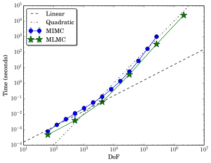
Figure 1. Average running time to estimate the difference operators for MIMC and MLMC versus the maximum number of degrees of freedom in those levels. Notice that MIMC has a higher cost than MLMC has for the same maximum number of degrees of freedom (DoF). This is because $2^{d}=8$ terms are estimated per difference level in MIMC compared with $2$ terms for difference levels in MLMC. Moreover, because all dimensions are isotropic in our numerical example, this shows that $\gamma_{i}$ in (13) is the same for $i=1\ldots d$ and ranges from 1 to 2.

3.2.2. MIMC Algorithm

The algorithm used to generate the results presented in the next section is a slight modification and extension of the MLMC algorithm first outlined in [12]. Specifically, the sample variance was used to calculate the required number of samples on each level in MIMC, with a minimum of $\overline{M_{0}}=5$ samples per level. Moreover, we used fixed tolerance-splitting, $\theta=0.5$. Note that this choice might be sub-optimal for MIMC and further work needs to be done in this case. The MIMC pseudo-algorithm can be summarized as follows

1. Set $k=1$

2. Ensure that at least $\overline{M_{0}}$ samples are calculated for all ${{{{\boldsymbol{\alpha}}}}}\in\mathcal{I}_{k}$.

3. Using sample variances as estimates for $V_{{{{\boldsymbol{\alpha}}}}}$, calculate $M_{{{{\boldsymbol{\alpha}}}}}$ according to (9) for all ${{{{\boldsymbol{\alpha}}}}}\in\mathcal{I}_{k}$.

4. Calculate extra samples to have at least $M_{{{{\boldsymbol{\alpha}}}}}$ samples for each ${{{{{\boldsymbol{\alpha}}}}}\in\mathcal{I}_{k}}$.

5. Estimate the bias. We expand on this step below.

6. Stop if the bias estimate is less than $(1-\theta)\mathrm{TOL}.$

7. Otherwise, increase $k$ and go to Step 2.

This algorithm assumes that $\mathcal{I}_{k}\subset\mathcal{I}_{k-1}$. For isotropic TD index sets, we simply use (33) with ${L=k/d}$. For full tensor index sets, we increase the value of each $L_{i}$ for $i=1,2,\ldots,d$ one at a time cyclically.

In Step 6, we use the following bias estimate:

(53) $$\text{Bias}(\mathcal{I}_{k})\approx\left|\sum_{\alpha\in\partial\mathcal{I}_{k}}{\mathrm{E}\mspace{-2.0mu}\left[{\Delta\mathscr{S}}_{\alpha}\right]}\right|,$$

where $\partial\mathcal{I}_{k}$ is the outer boundary of the index set, $\mathcal{I}_{k}$. Obviously, the error indicator (53) does not provide an error bound in general unless further assumptions on the integrand function $S$ are made. Nevertheless, we use this error indicator in our problem heuristically. We further approximate the expectations in (53) by sample averages using the $\max(\overline{M_{0}},M_{\alpha})$ samples that are available for every ${{{{\boldsymbol{\alpha}}}}}\in\partial\mathcal{I}_{k}$.

Finally, we apply the continuation concept from [10] by running MIMC (and MLMC) with a sequence of larger tolerances than $\mathrm{TOL}$ to obtain increasingly accurate estimates of the sample variances.

3.3. Results

Three methods were tested: MLMC as outlined in [8], MIMC with full tensor index sets (referred to as “FT” in the figures), and MIMC with isotropic total degree index sets (referred to as “TD” in the figures). In this isotropic example, the total degree index sets defined in Section 2.2 become

$$\mathcal{I}(L)=\{{{{{\boldsymbol{\alpha}}}}}\in\mathbb{N}^{3}:|{{{{\boldsymbol{\alpha}}}}}|\leq 3L\}.$$

Recall that in this example, $d=3,s_{i}=s=4,w_{i}=w=2$ and $\gamma_{i}=\gamma$ for all $i=1,2,3$, where $\gamma$ ranges from 1 to 2. As such, the condition for MLMC, $2w\geq\min(s,d\gamma)$, is satisfied for $\gamma\in[1,2]$. Similarly the condition for MIMC with the optimal TD index set, $2w\geq s$, is satisfied. On the other hand, the condition for MIMC with a full tensor index set, $2w>d\min(s,\gamma)$, is not satisfied for $\gamma\in\left[\frac{4}{3},2\right]$. According to Remark 2.2, for small enough tolerances where $\gamma=2$ mostly, we expect the work complexity of MIMC with a TD index set to be ${\mathcal{O}\left(\mathrm{TOL}^{-2}\right)}$. On the other hand, MIMC with a full tensor index set would have a work complexity of ${\mathcal{O}\left(\mathrm{TOL}^{-\frac{d\gamma}{w}}\right)}={\mathcal{O}\left(\mathrm{TOL}^{-3}\right)}$. Similarly, MLMC would have a work complexity of ${\mathcal{O}\left(\mathrm{TOL}^{-2-\frac{d\gamma-s}{w}}\right)}={\mathcal{O}\left(\mathrm{TOL}^{-3}\right)}$.

Figures 2 and 4 show that Assumptions 1-3 are indeed satisfied (at least for sufficiently fine discretizations). On the other hand, Figures 5 and 6 show numerical results that are in agreement with the convergence rates claimed above. Specifically, these figures show results consistent with the values $s=4$ and $w=2$. Moreover, Figure 4 shows numerical evidence of the normality of the statistical error of the MIMC estimator. Figure 7 shows the running time for different tolerances. The MIMC method with total degree index sets seems to exhibit the expected rate of $\mathrm{TOL}^{-2}$ in the computational time. On the other hand, MLMC and MIMC with a full tensor index set seem to exhibit a rate closer to $\mathrm{TOL}^{-3}$, especially for smaller tolerances. The staircase-like effect in running time of MLMC and MIMC with a full tensor index set is due to the discrete increments of the maximum number of degrees of freedom per level (cf. Figure 9). Since a fixed tolerance-splitting parameter, $\theta=0.5$, was used, the statistical constraint is not relaxed when the bias becomes smaller and the algorithm ends up solving for a slightly smaller tolerance than the required $\mathrm{TOL}$ (cf. Figure 9). Notice that although the fixed tolerance splitting parameter was also used for MIMC with total degree index sets, the running time does not exhibit the same jumps. This is because the discrete increments in the number of degrees of freedom are not as significant in this method (cf. Figure 9). Finally, Figure 9 can also be used to estimate the memory requirements of MIMC versus MLMC. In this figure we can see that using MIMC with total degree index sets, allows us to achieve the same value of $\mathrm{TOL}$ with substantially fewer degrees of freedom. In fact, we were not able to run MLMC or MIMC with full tensor index sets for very small tolerances due to their memory requirements.

For comparison, Figure 10 shows the running time of MLMC and MIMC with a TD index set when applied to a similar problem but in four dimensions instead of three. Here, we expect MLMC to have a work complexity of ${\mathcal{O}\left(\mathrm{TOL}^{-4}\right)}$ while the expected rate of MIMC with a TD index set is still ${\mathcal{O}\left(\mathrm{TOL}^{-2}\right)}$. The tolerances shown for MLMC were the only ones that we were able to compute with 64 gigabytes of memory.

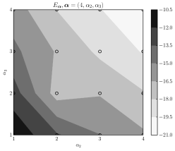
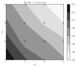
Figure 2. Numerical example, rate verification: contour plots of sample mean (left) and variance (right) of mixed differences used in MIMC for a slice of multi indices.

[] []

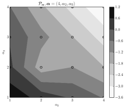
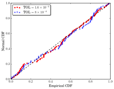
Figure 3. Numerical example, rate verification: contour plots of profits used in MIMC for a slice of multi indices. The parallel lines, asymptotically, suggest that isotropic TD index sets are nearly optimal in this example.

Figure 4. QQ-plot of the normalized error of the MIMC estimator with a TD index set for different values of $\mathrm{TOL}$. Similar results were obtained for other tolerances using either MLMC or MIMC with full tensor index sets. This is in agreement with Lemma A.1.

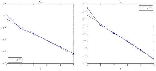
Figure 5. Numerical example, rate verification: sample mean (left) and variance (right) of differences versus level $\ell$ for MLMC. Notice that the observed rates are consistent with Remark 2.1.

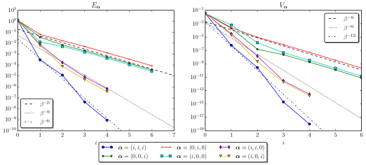
Figure 6. Numerical example, rate verification: sample mean (left) and variance (right) of mixed differences used in MIMC. Notice that the observed rates are consistent with Remark 2.1 and are better than those observed for MLMC, cf. Figure 5.

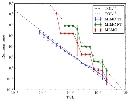
Figure 7. Running time for different values of $\mathrm{TOL}$ when using MLMC and MIMC with different index sets. The error bars extend from the 5% percentile to the 95% percentile. Notice that the rate of MIMC is the optimal Monte Carlo rate of ${\mathcal{O}\left(\mathrm{TOL}^{-2}\right)}$ for this example, while MLMC is closer to ${\mathcal{O}\left(\mathrm{TOL}^{-3}\right)}$, in agreement with the results listed in Remark 2.2 for $d=3,\gamma=2,s=4$ and $w=2$. For comparison, recall that MC has a work complexity of ${\mathcal{O}\left(\mathrm{TOL}^{-5}\right)}$.

[] []

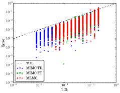
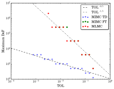
Figure 8. The exact computational error for MLMC and MIMC using different index sets. Notice that since we imposed a fixed tolerance splitting parameter, $\theta=0.5$, in some cases our numerical error is slightly smaller than the required $\mathrm{TOL}$ for all methods.

Figure 9. The maximum number of degrees of freedom across levels for MLMC and MIMC with different index sets. Notice that by using total degree index sets, we are able to achieve the same value of $\mathrm{TOL}$ with substantially fewer degrees of freedom. Refer to Remark 2.6 for discussions regarding this point.

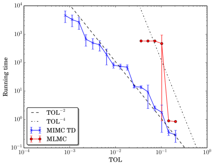
Figure 10. Running time for different values of $\mathrm{TOL}$ for a 4D problem when using MLMC and MIMC with TD index sets. The error bars extend from the 5% percentile to the 95% percentile. Notice that the work complexity of MIMC for this example has the optimal Monte Carlo rate of ${\mathcal{O}\left(\mathrm{TOL}^{-2}\right)}$. According to Remark 2.2 for $d=3,\gamma=2,s=4$ and $w=2$, MLMC is expected to have a work complexity of ${\mathcal{O}\left(\mathrm{TOL}^{-4}\right)}$. However, we were not able to compute for smaller tolerances with 64 gigabytes of available memory. For comparison, recall that MC has a work complexity of ${\mathcal{O}\left(\mathrm{TOL}^{-6}\right)}$.

4. Conclusions

We have proposed and analyzed a novel Multi-Index Monte Carlo (MIMC) method for weak approximation of stochastic models that are described in terms of differential equations either driven by random measures or with random coefficients. The MIMC method uses a stochastic combination technique to solve the given approximation problem, generalizing the notion of standard MLMC levels into a set of multi indices that should be properly chosen to exploit the available regularity. Indeed, instead of using first-order differences as in standard MLMC, MIMC uses high-order differences to reduce the variance of the hierarchical differences dramatically. This in turn gives a new improved complexity result that increases the domain of the problem parameters for which the method achieves the optimal convergence rate, $\mathcal{O}(\mathrm{TOL}^{-2}).$ We have outlined a method for constructing an optimal index set of indices for our MIMC method. Moreover, under our standard assumptions, we showed that the optimal index set turns out to be the total degree (TD) type. Using optimal index sets, MIMC achieves a better rate for the computational complexity than when using full tensor index sets; in fact, the rate does not depend on the dimensionality of the underlying problem, up to logarithmic factors. Similarly, the rate of required memory for MIMC with respect to $\mathrm{TOL}$ is, up to a logarithmic terms, dimension-independent (unlike MLMC) allowing us to solve for smaller tolerances than is possible with MLMC. In addition, for MIMC with TD index sets, the conditions on the weak convergence rate for achieving such rates are dimension-independent and less stringent, compared with similar conditions for MLMC and MIMC with full tensor index sets. We also presented numerical results to substantiate some of the derived computational complexity rates. In Appendix A, using the Lindeberg-Feller theorem, we also show the asymptotic normality of the statistical error in the MIMC estimator and justify in this way our error estimate that allows both the required accuracy and confidence level in the final result to be prescribed.

Our method requires more regularity of the underlying solution than does MLMC. If the underlying solution is sufficiently regular only in some directions, then one can still combine MIMC with MLMC by applying mixed first-order differences to the sufficiently regular directions, while applying a single first-order difference to less regular directions.

In future work, more has to be done to improve the MIMC algorithm, using the variance convergence model to estimate the variances instead of relying on sample variance only; for example, by applying ideas such as those in [10]. Also, a better choice of the splitting parameter, $\theta$, can be derived to improve the computational complexity up to a constant factor; similar to the work done in [17]. Moreover, MIMC can be used to improve the computational complexity rate in the case of PDEs with random fields that are approximated by converging series, such as a Karhunen-Loéve decomposition, cf. [31]. By treating the number of terms in the decomposition as an extra discretization direction and applying MIMC, we might be able to improve the computational complexity. Also, the use of either a priori refined non-uniform discretizations or adaptive algorithms based on a posteriori error estimates for non-uniform refinement as introduced in [22, 23, 27] can be combined with MIMC to improve efficiency. Finally, ideas from [32] and [18] can be extended by replacing the Monte Carlo sampling of mixed differences in MIMC by a sparse-grid stochastic collocation, effectively including interpolation levels along the different random directions into the combination technique together with the other discretization parameters. Similarly, we can apply Quasi Monte Carlo to replace Monte Carlo sampling of the mixed differences in MIMC as outlined in [25] for a multilevel setting. Provided that there is enough mixed regularity in the problem at hand, we expect to improve again the optimal complexity further from $\mathcal{O}(\mathrm{TOL}^{-2})$ in MIMC to $\mathcal{O}(\mathrm{TOL}^{-r})$ with $r<2$.

Appendix A Asymptotic Normality of the MIMC estimator

Lemma A.1 (Asymptotic Normality of the MIMC Estimator).

Consider the MIMC estimator introduced in (2), $\mathcal{A}$, based on a set of multi indices, $\mathcal{I}(\mathrm{TOL})$, and given by

$$\mathcal{A}=\sum_{{{{{\boldsymbol{\alpha}}}}}\in\mathcal{I}}\sum_{m=1}^{M_{{{{\boldsymbol{\alpha}}}}}}\frac{{\Delta\mathscr{S}}_{{{{{\boldsymbol{\alpha}}}}}}(\omega_{{{{{\boldsymbol{\alpha}}}}},m})}{M_{{{{\boldsymbol{\alpha}}}}}}.$$

Assume that for $1\leq i\leq d$ there exists $0<L_{i}(\mathrm{TOL})$ such that

(54) $$\mathcal{I}(\mathrm{TOL})\subset\{{{{{\boldsymbol{\alpha}}}}}\in\mathbb{N}^{d}:\alpha_{i}\leq L_{i}(\mathrm{TOL}),\text{ for }1\leq i\leq d\}.$$

Denote ${Y_{{{{\boldsymbol{\alpha}}}}}=|{\Delta\mathscr{S}}_{{{{\boldsymbol{\alpha}}}}}-{\mathrm{E}\mspace{-2.0mu}\left[{\Delta\mathscr{S}}_{{{{\boldsymbol{\alpha}}}}}\right]}|}$ and assume that the following inequalities

(55a) $$Q_{S}\prod_{i=1}^{d}\exp(-\alpha_{i}s_{i}) \leq{\mathrm{E}\mspace{-2.0mu}\left[Y_{{{{{\boldsymbol{\alpha}}}}}}^{2}\right]},$$

(55b) $${\mathrm{E}\mspace{-2.0mu}\left[Y_{{{{{\boldsymbol{\alpha}}}}}}^{2+\rho}\right]} \leq Q_{R}\prod_{i=1}^{d}\exp(-\alpha_{i}r_{i}),$$

hold for strictly positive constants $\rho,\{s_{i},r_{i}\}_{i=1}^{d},Q_{S}$ and $Q_{R}$. Choose the number of samples on each level, $M_{{{{\boldsymbol{\alpha}}}}}(\mathrm{TOL})$, to satisfy, for strictly positive sequences $\{\tilde{s}_{i}\}_{i=1}^{d}$ and $\{H_{{{\boldsymbol{\tau}}}}\}_{{{{\boldsymbol{\tau}}}}\in\mathcal{I}(\mathrm{TOL})}$ and for all ${{{{\boldsymbol{\alpha}}}}}\in\mathcal{I}(\mathrm{TOL})$,

(56) $$M_{{{{\boldsymbol{\alpha}}}}}\geq\mathrm{TOL}^{-2}\,C_{M}\left(\prod_{i=1}^{d}\exp(-\alpha_{i}\tilde{s}_{i})\right)H_{{{{\boldsymbol{\alpha}}}}}^{-1}\left(\sum_{{{{\boldsymbol{\tau}}}}\in\mathcal{I}(\mathrm{TOL})}H_{{{\boldsymbol{\tau}}}}\right).$$

Denote, for all $1\leq i\leq d,$

(57) $$p_{i}=(\rho/2)\tilde{s}_{i}-r_{i}+(1+\rho/2)s_{i}$$

and choose $0<c_{i}$ such that whenever $0<p_{i}$, the inequality $c_{i}<\rho/p_{i}$ holds. Finally, if we take the quantities $L_{i}(\mathrm{TOL})$ in (54) to be

$$L_{i}(\mathrm{TOL})=c_{i}\log(\mathrm{TOL}^{-1})+{o\left(\log(\mathrm{TOL}^{-1})\right)},\text{ for all }1\leq i\leq d,$$

then we have

$$\lim_{\mathrm{TOL}\downarrow 0}{\mathrm{P}\mspace{-2.0mu}\left[\frac{\mathcal{A}-{\mathrm{E}\mspace{-2.0mu}\left[\mathcal{A}\right]}}{\sqrt{{\mathrm{Var}\mspace{-2.0mu}\left[\mathcal{A}\right]}}}\leq z\right]}=\Phi\left(z\right),$$

where $\Phi(z)$ is the normal cumulative distribution function of a standard normal random variable.

Proof.

We prove this theorem by ensuring that the Lindeberg condition [11, Lindeberg-Feller Theorem, p. 114] (also restated in [10, Theorem A.1]) is satisfied. The condition becomes in this case

$$\lim_{\mathrm{TOL}\downarrow 0}\underbrace{\frac{1}{{\mathrm{Var}\mspace{-2.0mu}\left[\mathcal{A}\right]}}\sum_{{{{{\boldsymbol{\alpha}}}}}\in\mathcal{I}(\mathrm{TOL})}\sum_{m=1}^{M_{{{{\boldsymbol{\alpha}}}}}}{\mathrm{E}\mspace{-2.0mu}\left[\frac{Y_{{{{\boldsymbol{\alpha}}}}}^{2}}{M_{{{{\boldsymbol{\alpha}}}}}^{2}}\mathbf{1}_{\frac{Y_{{{{\boldsymbol{\alpha}}}}}}{M_{{{{\boldsymbol{\alpha}}}}}}>\epsilon\sqrt{{\mathrm{Var}\mspace{-2.0mu}\left[\mathcal{A}\right]}}}\right]}}_{=F}=0,$$

for all $\epsilon>0$. Below we make repeated use of the following identity for non-negative sequences ${\{a_{{{{\boldsymbol{\alpha}}}}}\}}$ and ${\{b_{{{{\boldsymbol{\alpha}}}}}\}}$ and $q\geq 0$:

(58) $$\sum_{{{{{\boldsymbol{\alpha}}}}}}{a_{{{{\boldsymbol{\alpha}}}}}^{q}b_{{{{\boldsymbol{\alpha}}}}}}\leq\left(\sum_{{{{\boldsymbol{\alpha}}}}}a_{{{{\boldsymbol{\alpha}}}}}\right)^{q}\sum_{{{{\boldsymbol{\alpha}}}}}b_{{{{\boldsymbol{\alpha}}}}}.$$

First, we use the Markov inequality to bound

$$F =\frac{1}{{\mathrm{Var}\mspace{-2.0mu}\left[\mathcal{A}\right]}}\sum_{{{{{\boldsymbol{\alpha}}}}}\in\mathcal{I}(\mathrm{TOL})}\sum_{m=1}^{M_{{{{\boldsymbol{\alpha}}}}}}{\mathrm{E}\mspace{-2.0mu}\left[\frac{Y_{{{{\boldsymbol{\alpha}}}}}^{2}}{M_{{{{\boldsymbol{\alpha}}}}}^{2}}\mathbf{1}_{Y_{{{{\boldsymbol{\alpha}}}}}>\epsilon\sqrt{{\mathrm{Var}\mspace{-2.0mu}\left[\mathcal{A}\right]}}M_{{{{\boldsymbol{\alpha}}}}}}\right]}$$

$$\leq\frac{\epsilon^{-\rho}}{{\mathrm{Var}\mspace{-2.0mu}\left[\mathcal{A}\right]}^{1+\rho/2}}\sum_{{{{{\boldsymbol{\alpha}}}}}\in\mathcal{I}(\mathrm{TOL})}M_{{{{\boldsymbol{\alpha}}}}}^{-1-\rho}{\mathrm{E}\mspace{-2.0mu}\left[Y_{{{{\boldsymbol{\alpha}}}}}^{2+\rho}\right]}.$$

Using (58) and substituting for the variance ${\mathrm{Var}\mspace{-2.0mu}\left[\mathcal{A}\right]}$ where we denote ${\mathrm{Var}\mspace{-2.0mu}\left[{\Delta\mathscr{S}}_{{{{\boldsymbol{\alpha}}}}}\right]}={\mathrm{E}\mspace{-2.0mu}\left[\left(\Delta\mathcal{S}_{{{{\boldsymbol{\alpha}}}}}-{\mathrm{E}\mspace{-2.0mu}\left[\Delta\mathcal{S}_{{{{\boldsymbol{\alpha}}}}}\right]}\right)^{2}\right]}$ by $V_{{{{\boldsymbol{\alpha}}}}}$, we find

$$F \leq\frac{\epsilon^{-\rho}\left(\sum_{{{{{\boldsymbol{\alpha}}}}}\in\mathcal{I}(\mathrm{TOL})}M_{{{{\boldsymbol{\alpha}}}}}^{-1}V_{{{{\boldsymbol{\alpha}}}}}\right)^{1+\rho/2}}{\left(\sum_{{{{{\boldsymbol{\alpha}}}}}\in\mathcal{I}(\mathrm{TOL})}V_{{{{\boldsymbol{\alpha}}}}}M_{{{{\boldsymbol{\alpha}}}}}^{-1}\right)^{1+\rho/2}}\sum_{{{{{\boldsymbol{\alpha}}}}}\in\mathcal{I}(\mathrm{TOL})}V_{{{{\boldsymbol{\alpha}}}}}^{-1-\rho/2}M_{{{{\boldsymbol{\alpha}}}}}^{-\rho/2}{\mathrm{E}\mspace{-2.0mu}\left[Y_{{{{\boldsymbol{\alpha}}}}}^{2+\rho}\right]}$$

$$=\epsilon^{-\rho}\sum_{{{{{\boldsymbol{\alpha}}}}}\in\mathcal{I}(\mathrm{TOL})}V_{{{{\boldsymbol{\alpha}}}}}^{-1-{\rho}/{2}}M_{{{{\boldsymbol{\alpha}}}}}^{-{\rho}/{2}}{\mathrm{E}\mspace{-2.0mu}\left[Y_{{{{\boldsymbol{\alpha}}}}}^{2+\rho}\right]}.$$

Using the lower bound in (56) on the number of samples, $M_{{{{\boldsymbol{\alpha}}}}}$, and (58), again yields

$$F \leq C_{M}^{-\rho/2}\epsilon^{-\rho}\mathrm{TOL}^{\rho}\left(\sum_{{{{{\boldsymbol{\alpha}}}}}\in\mathcal{I}(\mathrm{TOL})}V_{{{{\boldsymbol{\alpha}}}}}^{-1-{\rho}/{2}}\left(\prod_{i=1}^{d}\exp\left(\frac{\rho\alpha_{i}\tilde{s}_{i}}{2}\right)\right)H_{{{{\boldsymbol{\alpha}}}}}^{\rho/2}{\mathrm{E}\mspace{-2.0mu}\left[Y_{{{{\boldsymbol{\alpha}}}}}^{2+\rho}\right]}\right)$$

$$\hskip 80.00012pt\left(\sum_{{{{\boldsymbol{\tau}}}}\in\mathcal{I}(\mathrm{TOL})}H_{{{\boldsymbol{\tau}}}}\right)^{-\rho/2}$$

$$\leq C_{M}^{-\rho/2}\epsilon^{-\rho}\mathrm{TOL}^{\rho}\left(\sum_{{{{{\boldsymbol{\alpha}}}}}\in\mathcal{I}(\mathrm{TOL})}V_{{{{\boldsymbol{\alpha}}}}}^{-1-{\rho}/{2}}\left(\prod_{i=1}^{d}\exp\left(\frac{\rho\alpha_{i}\tilde{s}_{i}}{2}\right)\right){\mathrm{E}\mspace{-2.0mu}\left[Y_{{{{\boldsymbol{\alpha}}}}}^{2+\rho}\right]}\right).$$

Finally, using the bounds (55a) and (55b),

$$F \leq\underbrace{C_{M}^{-\rho/2}\epsilon^{-\rho}Q_{S}^{-1-{\rho}/{2}}Q_{R}}_{=C_{F}}\mathrm{TOL}^{\rho}\left(\sum_{{{{{\boldsymbol{\alpha}}}}}\in\mathcal{I}(\mathrm{TOL})}\left(\prod_{i=1}^{d}\exp\left(p_{i}\alpha_{i}\right)\right)\right).$$

Next, define three sets of dimension indices:

$$\hat{I}_{1} =\{1\leq i\leq d:p_{i}<0\},$$

$$\hat{I}_{2} =\{1\leq i\leq d:p_{i}=0\},$$

$$\hat{I}_{3} =\{1\leq i\leq d:p_{i}>0\}.$$

Then, using (54) yields

$$F\leq C_{F}\mathrm{TOL}^{\rho}\prod_{i=1}^{d}\left(\sum_{\alpha_{i}=0}^{L_{i}}\exp\left(p_{i}\alpha_{i}\right)\right)$$

$$\leq C_{F}\mathrm{TOL}^{\rho}\prod_{i\in\hat{I}_{1}}\frac{1}{1-\exp(p_{i})}\prod_{i\in\hat{I}_{2}}L_{i}\prod_{i\in\hat{I}_{3}}\frac{1-\exp(p_{i}(L_{i}+1))}{1-\exp(p_{i})}.$$

To conclude, observe that if $|\hat{I}_{3}|=0$, then $\lim_{\mathrm{TOL}\downarrow 0}F=0$ for any choice of $L_{i}\geq 0$, $1\leq i\leq d$. Similarly, if $|\hat{I}_{3}|>0$, since we assumed that $c_{i}p_{i}<\rho$ holds for all $i\in\hat{I}_{3}$, then $\lim_{\mathrm{TOL}\downarrow 0}F=0$. ∎

Remark.

The lower bound on the number of samples per index (56) mirrors choice (9), the latter being the optimal number of samples satisfying constraint (7). Specifically, $H_{{{{\boldsymbol{\alpha}}}}}=\sqrt{V_{{{{\boldsymbol{\alpha}}}}}W_{{{{\boldsymbol{\alpha}}}}}}$ and $\tilde{s}_{i}=s_{i}$. Furthermore, notice that the previous Lemma bounds the growth of $L$ from above, while Theorem 2.1 and Theorem 2.2 bound the value of $L$ from below to satisfy the bias accuracy constraint.

Appendix B Integrating an exponential over a simplex

Lemma B.1.

The following identity holds for any $L>0$ and $a\in\mathbb{R}$:

(59) $${\int_{\{{{\boldsymbol{x}}}\in\mathbb{R}_{+}^{d}\>:\>|{{\boldsymbol{x}}}|\leq L\}}}\exp(a|{{\boldsymbol{x}}}|)\textnormal{d}{{\boldsymbol{x}}} =(-a)^{-d}\left(1-\exp(La)\sum_{j=0}^{d-1}\frac{(-La)^{j}}{j!}\right)$$

$$=\frac{1}{(d-1)!}\int_{0}^{L}\exp(at)t^{d-1}\>\textnormal{d}t.$$

Proof.

$${\int_{\{{{\boldsymbol{x}}}\in\mathbb{R}_{+}^{d}\>:\>|{{\boldsymbol{x}}}|\leq L\}}}\exp(a|{{\boldsymbol{x}}}|)\textnormal{d}{{\boldsymbol{x}}} =L^{d}{\int_{\{{{\boldsymbol{x}}}\in\mathbb{R}_{+}^{d}\>:\>|{{\boldsymbol{x}}}|\leq 1\}}}\exp(aL|{{\boldsymbol{x}}}|)\textnormal{d}{{\boldsymbol{x}}}.$$

Then, we prove, by induction on $d$ and for $b=aL$, the following identity:

$${\int_{\{{{\boldsymbol{x}}}\in\mathbb{R}_{+}^{d}\>:\>|{{\boldsymbol{x}}}|\leq 1\}}}\exp(b|{{\boldsymbol{x}}}|)\textnormal{d}{{{\boldsymbol{x}}}}=(-b)^{-d}\left(1-\exp(b)\sum_{j=0}^{d-1}\frac{(-b)^{j}}{j!}\right).$$

First, for $d=1$, we have

$$\int_{0}^{1}\exp(bx)\textnormal{d}x=\frac{\exp(b)-1}{b}.$$

Next, assuming that the identity is true for $d-1$, we prove it for $d$. Indeed, we have

$${\int_{\{{{\boldsymbol{x}}}\in\mathbb{R}_{+}^{d}\>:\>|{{\boldsymbol{x}}}|\leq 1\}}}\exp(b|{{\boldsymbol{x}}}|)\textnormal{d}{{\boldsymbol{x}}}$$

$$=\int_{0}^{1}\exp(by)\left({\int_{\{{{\boldsymbol{x}}}\in\mathbb{R}_{+}^{d-1}\>:\>|{{\boldsymbol{x}}}|\leq 1-y\}}}\exp(b|{{\boldsymbol{x}}}|)\textnormal{d}{{\boldsymbol{x}}}\right)\textnormal{d}y$$

$$=\int_{0}^{1}\exp(by)\left(1-y\right)^{d-1}\left({\int_{\{{{\boldsymbol{x}}}\in\mathbb{R}_{+}^{d-1}\>:\>|{{\boldsymbol{x}}}|\leq 1\}}}\exp((1-y)b|{{\boldsymbol{x}}}|)\textnormal{d}{{\boldsymbol{x}}}\right)\textnormal{d}y$$

$$=\int_{0}^{1}\exp(by)\frac{\left(1-y\right)^{d-1}}{(-(1-y)b)^{d-1}}\left(1-\exp((1-y)b)\sum_{j=0}^{d-2}\frac{(-(1-y)b)^{j}}{j!}\right)\textnormal{d}y$$

$$=\int_{0}^{1}\left[\frac{\exp(by)}{(-b)^{d-1}}-\frac{\exp(b)}{(-b)^{d-1}}\sum_{j=0}^{d-2}\frac{(-(1-y)b)^{j}}{j!}\right]\textnormal{d}y$$

$$=\frac{\left(-1\right)^{d-1}}{b^{d}}\left(\exp(b)-1\right)-\frac{(-1)^{d-1}\exp(b)}{b^{d-1}}\sum_{j=0}^{d-2}\frac{(-b)^{j}}{(j+1)!}$$

$$=\frac{\left(-1\right)^{d}}{b^{d}}-\frac{\left(-1\right)^{d}}{b^{d}}\exp(b)-\frac{(-1)^{d}\exp(b)}{b^{d}}\sum_{j=1}^{d-1}\frac{(-b)^{j}}{(j)!}$$

$$=(-b)^{-d}\left(1-\exp(b)\sum_{j=0}^{d-1}\frac{(-b)^{j}}{j!}\right).$$

Finally, the second equality in (59) follows by repeatedly integrating by parts. ∎

Lemma B.2.

For $a\in\mathbb{R}^{d}$, assume $A=\max_{i=1,2\ldots d}a_{i}>0$ and denote

$$\mathfrak{a}_{1} =\#\left\{i=1,2,\ldots d\>:\>a_{i}=A\right\},\qquad \mathfrak{a}_{2} =d-\mathfrak{a}_{1}.$$

Then, for any $L>0$, there exists an $\epsilon>0$ satisfying

$$\epsilon\leq A-\max\left(0,\max_{\begin{subarray}{c}i=1,2\ldots d\\ a_{i}<A\end{subarray}}a_{i}\right),$$

such that the following inequality holds:

(60) $${\int_{\{{{\boldsymbol{x}}}\in\mathbb{R}_{+}^{d}\>:\>|{{\boldsymbol{x}}}|\leq L\}}}\exp({{\boldsymbol{a}}}\cdot{{\boldsymbol{x}}})\textnormal{d}{{\boldsymbol{x}}} \leq\mathfrak{C_{W}}({{\boldsymbol{a}}})\exp\left(AL\right)L^{\mathfrak{a}_{1}-1}.$$

Here, the constant $\mathfrak{C_{W}}({{\boldsymbol{a}}})$ is given by

(61) $$\mathfrak{C_{W}}({{\boldsymbol{a}}})=\begin{cases}\frac{1}{A(d-1)!}&\text{ if $\mathfrak{a}_{1}=d$}\\ \frac{4}{\epsilon(2A-\epsilon)}\frac{\exp(1-\mathfrak{a}_{2})}{(\mathfrak{a}_{1}-1)!(\mathfrak{a}_{2}-1)!}\left(\frac{2(\mathfrak{a}_{2}-1)}{\epsilon}\right)^{\mathfrak{a}_{2}-1}&\text{otherwise}\end{cases}$$

Proof.

First, note that ${{\boldsymbol{a}}}=A{{\boldsymbol{1}}}$ for some scalar $A>0$ and ${{\boldsymbol{1}}}=(1,1,\ldots,1)$ if and only if $\mathfrak{a}_{1}=d$. Then Lemma B.1 immediately gives

$${\int_{\{{{\boldsymbol{x}}}\in\mathbb{R}_{+}^{d}\>:\>|{{\boldsymbol{x}}}|\leq L\}}}\exp({{\boldsymbol{a}}}\cdot{{\boldsymbol{x}}})\textnormal{d}{{\boldsymbol{x}}}\leq\frac{L^{d-1}\exp(AL)}{A(d-1)!}.$$

Otherwise, recall that

(62) $$x^{j}\leq\left(\frac{j}{b}\right)^{j}\exp(-j)\exp(bx)$$

holds for any $x>0,b>0$ and $j\in\mathbb{N}$. Then, using Lemma B.1 and (62), we can write

$${\int_{\{{{\boldsymbol{x}}}\in\mathbb{R}_{+}^{d}\>:\>|{{\boldsymbol{x}}}|\leq L\}}}\exp({{{\boldsymbol{a}}}}\cdot{{\boldsymbol{x}}})\textnormal{d}{{\boldsymbol{x}}}$$

$$\leq{\int_{\{{{\boldsymbol{x}}}_{2}\in\mathbb{R}_{+}^{\mathfrak{a}_{2}}\>:\>|{{\boldsymbol{x}}}_{2}|\leq L\}}}\exp\left(\left(A-\epsilon\right)|{{\boldsymbol{x}}}_{2}|\right)\left({\int_{\{{{\boldsymbol{x}}}_{1}\in\mathbb{R}_{+}^{\mathfrak{a}_{1}}\>:\>|{{\boldsymbol{x}}}_{1}|\leq L-|{{\boldsymbol{x}}}_{2}|\}}}\exp(A|{{\boldsymbol{x}}}_{1}|)\textnormal{d}{{\boldsymbol{x}}}_{1}\right)\textnormal{d}{{\boldsymbol{x}}}_{2}$$

$$=\frac{1}{(\mathfrak{a}_{1}-1)!}{\int_{\{{{\boldsymbol{x}}}_{2}\in\mathbb{R}_{+}^{\mathfrak{a}_{2}}\>:\>|{{\boldsymbol{x}}}_{2}|\leq L\}}}\exp\left((A-\epsilon)|{{\boldsymbol{x}}}_{2}|\right)\left(\int_{0}^{L-|{{\boldsymbol{x}}}_{2}|}\exp(At)t^{\mathfrak{a}_{1}-1}\textnormal{d}t\right)\textnormal{d}{{\boldsymbol{x}}}_{2}$$

$$=\frac{1}{(\mathfrak{a}_{1}-1)!}\int_{0}^{L}\exp(At)t^{\mathfrak{a}_{1}-1}\left({\int_{\{{{\boldsymbol{x}}}_{2}\in\mathbb{R}_{+}^{\mathfrak{a}_{2}}\>:\>|{{\boldsymbol{x}}}_{2}|\leq L-t\}}}\exp\left((A-\epsilon)|{{\boldsymbol{x}}}_{2}|\right)\textnormal{d}{{\boldsymbol{x}}}_{2}\right)\textnormal{d}t$$

$$=\frac{1}{(\mathfrak{a}_{1}-1)!(\mathfrak{a}_{2}-1)!}\int_{0}^{L}\exp(At)t^{\mathfrak{a}_{1}-1}\left(\int_{0}^{L-t}\exp\left((A-\epsilon)z\right)z^{\mathfrak{a}_{2}-1}\textnormal{d}z\right)\textnormal{d}t$$

$$\leq{\mathfrak{C}}\int_{0}^{L}\exp(At)t^{\mathfrak{a}_{1}-1}\left(\int_{0}^{L-t}\exp\left(\frac{z(2A-\epsilon)}{2}\right)\textnormal{d}z\right)\textnormal{d}t,$$

$$\text{where}\qquad{\mathfrak{C}}=\frac{\exp(1-\mathfrak{a}_{2})}{(\mathfrak{a}_{1}-1)!(\mathfrak{a}_{2}-1)!}\left(\frac{2(\mathfrak{a}_{2}-1)}{\epsilon}\right)^{\mathfrak{a}_{2}-1},$$

continuing

$${\int_{\{{{\boldsymbol{x}}}\in\mathbb{R}_{+}^{d}\>:\>|{{\boldsymbol{x}}}|\leq L\}}}\exp({{{\boldsymbol{a}}}}\cdot{{\boldsymbol{x}}})\textnormal{d}{{\boldsymbol{x}}}$$

$$\leq{\mathfrak{C}}\exp\left(\frac{L(2A-\epsilon)}{2}\right)\frac{2}{2A-\epsilon}\int_{0}^{L}t^{\mathfrak{a}_{1}-1}\exp\left(\frac{\epsilon t}{2}\right)\textnormal{d}t$$

$$\leq{\mathfrak{C}}\exp\left(\frac{L(2A-\epsilon)}{2}\right)\frac{2L^{\mathfrak{a}_{1}-1}}{2A-\epsilon}\int_{0}^{L}\exp\left(\frac{\epsilon t}{2}\right)\textnormal{d}t$$

$$\leq\frac{4{\mathfrak{C}}}{\epsilon(2A-\epsilon)}\exp\left(AL\right)L^{\mathfrak{a}_{1}-1}.$$

∎

Lemma B.3.

The following inequality holds for any $L\geq 1$ and ${{\boldsymbol{a}}}\in\mathbb{R}_{+}^{d}$:

$${\int_{\{{{\boldsymbol{x}}}\in\mathbb{R}_{+}^{d}\>:\>|{{\boldsymbol{x}}}|>L\}}}\exp(-{{\boldsymbol{a}}}\cdot{{\boldsymbol{x}}})\textnormal{d}{{\boldsymbol{x}}} \leq\mathfrak{C_{B}}({{\boldsymbol{a}}})\exp\left(-AL\right)L^{\mathfrak{a}_{1}-1},$$

where

(63) $$\mathfrak{C_{B}}({{\boldsymbol{a}}})=\begin{cases}\sum_{j=0}^{d-1}\frac{A^{j-d}}{j!}&\text{ if $\mathfrak{a}_{1}=d$}\\ {\left(A+\epsilon\right)}^{-\mathfrak{a}_{2}}\sum_{j=0}^{\mathfrak{a}_{1}-1}\frac{A^{j-\mathfrak{a}_{1}}}{j!}+\frac{2\sum_{j=0}^{\mathfrak{a}_{2}-1}\exp(-j)\left(\frac{2j}{\epsilon}\right)^{j}\frac{{\left(A+\epsilon\right)}^{j-\mathfrak{a}_{2}}}{j!}}{(\mathfrak{a}_{1}-1)!\epsilon}&\text{otherwise}\end{cases}$$

and

$$A =\min_{i=1,2\ldots d}a_{i},\qquad\epsilon=\min_{\begin{subarray}{c}i=1,2\ldots d\\ a_{i}>A\end{subarray}}a_{i}-A,$$

$$\mathfrak{a}_{1} =\#\left\{i=1,2,\ldots d\>:\>a_{i}=A\right\}.$$

$$\mathfrak{a}_{2} =d-\mathfrak{a}_{1}.$$

Proof.

First, note that ${{\boldsymbol{a}}}=A{{\boldsymbol{1}}}$ for some scalar $A>0$ and ${{\boldsymbol{1}}}=(1,1,\ldots,1)$ if and only if $\mathfrak{a}_{1}=d$. Then Lemma B.1 immediately gives:

$${\int_{\{{{\boldsymbol{x}}}\in\mathbb{R}_{+}^{d}\>:\>|{{\boldsymbol{x}}}|>L\}}}\exp(-A|{{\boldsymbol{x}}}|)\textnormal{d}{{\boldsymbol{x}}}$$

$$=\int_{{{\boldsymbol{x}}}\in\mathbb{R}_{+}^{d}}\exp(-A|{{\boldsymbol{x}}}|)\textnormal{d}{{\boldsymbol{x}}}-{\int_{\{{{\boldsymbol{x}}}\in\mathbb{R}_{+}^{d}\>:\>|{{\boldsymbol{x}}}|\leq L\}}}\exp(-A|{{\boldsymbol{x}}}|)\textnormal{d}{{\boldsymbol{x}}}$$

$$=A^{-d}-A^{-d}\left(1-\exp(-AL)\sum_{j=0}^{d-1}\frac{(AL)^{j}}{j!}\right)$$

$$\leq\exp(-AL)L^{d-1}\sum_{j=0}^{d-1}\frac{A^{j-d}}{j!}$$

Otherwise, without loss of generality, assume that $a_{i}\leq a_{j}$ for all $1\leq i\leq j\leq d$. Then, again using Lemma B.1, we can write

$${\int_{\{{{\boldsymbol{x}}}\in\mathbb{R}_{+}^{d}\>:\>|{{\boldsymbol{x}}}|\geq L\}}}\exp\left(-\sum_{i=1}^{d}a_{i}x_{i}\right)\>\textnormal{d}{{\boldsymbol{x}}}$$

$$\leq{\int_{\{{{\boldsymbol{x}}}\in\mathbb{R}_{+}^{d}\>:\>|{{\boldsymbol{x}}}|\geq L\}}}\exp\left(-A\sum_{i=1}^{\mathfrak{a}_{1}}x_{i}-{\left(A+\epsilon\right)}\sum_{i=\mathfrak{a}_{1}+1}^{d}x_{i}\right)\>\textnormal{d}{{\boldsymbol{x}}}$$

$$=\Bigg{[}\int_{{{\boldsymbol{x}}}\in\mathbb{R}_{+}^{d}}\exp\left(-A\sum_{i=1}^{\mathfrak{a}_{1}}x_{i}-{\left(A+\epsilon\right)}\sum_{i=\mathfrak{a}_{1}+1}^{d}x_{i}\right)\textnormal{d}{{\boldsymbol{x}}}-$$

$$\hskip 60.00009pt{\int_{\{{{\boldsymbol{x}}}\in\mathbb{R}_{+}^{d}\>:\>|{{\boldsymbol{x}}}|\leq L\}}}\exp\left(-A\sum_{i=1}^{\mathfrak{a}_{1}}x_{i}-{\left(A+\epsilon\right)}\sum_{i=\mathfrak{a}_{1}+1}^{d}x_{i}\right)\>\textnormal{d}{{\boldsymbol{x}}}\Bigg{]},$$

where

$$\int_{{{\boldsymbol{x}}}\in\mathbb{R}_{+}^{d}}\exp\left(-A\sum_{i=1}^{\mathfrak{a}_{1}}x_{i}-(A+\epsilon)\sum_{i=\mathfrak{a}_{1}+1}^{d}x_{i}\right)\textnormal{d}{{\boldsymbol{x}}}=A^{-\mathfrak{a}_{1}}{\left(A+\epsilon\right)}^{-\mathfrak{a}_{2}}.$$

Now consider

$${\int_{\{{{\boldsymbol{x}}}\in\mathbb{R}_{+}^{d}\>:\>|{{\boldsymbol{x}}}|\leq L\}}}\exp\left(-A\sum_{i=1}^{\mathfrak{a}_{1}}x_{i}-{\left(A+\epsilon\right)}\sum_{i=\mathfrak{a}_{1}+1}^{d}x_{i}\right)\>\textnormal{d}{{\boldsymbol{x}}}$$

$$={\int_{\{{{\boldsymbol{x}}}_{2}\in\mathbb{R}_{+}^{\mathfrak{a}_{2}}\>:\>|{{\boldsymbol{x}}}_{2}|\leq L\}}}\exp\left(-{\left(A+\epsilon\right)}|{{\boldsymbol{x}}}_{2}|\right)$$

$$\hskip 60.00009pt\left({\int_{\{{{\boldsymbol{x}}}_{1}\in\mathbb{R}_{+}^{\mathfrak{a}_{1}}\>:\>|{{\boldsymbol{x}}}_{1}|\leq L-|{{\boldsymbol{x}}}_{2}|\}}}\exp\left(-A|{{\boldsymbol{x}}}_{1}|\right)\>\textnormal{d}{{\boldsymbol{x}_{1}}}\right)\>\textnormal{d}{{\boldsymbol{x}_{2}}}$$

$$=\frac{1}{(\mathfrak{a}_{1}-1)!}{\int_{\{{{\boldsymbol{x}}}_{2}\in\mathbb{R}_{+}^{\mathfrak{a}_{2}}\>:\>|{{\boldsymbol{x}}}_{2}|\leq L\}}}\exp\left(-{\left(A+\epsilon\right)}|{{\boldsymbol{x}}}_{2}|\right)\left(\int_{0}^{L-|{{\boldsymbol{x}}}_{2}|}\exp(-At)t^{\mathfrak{a}_{1}-1}\textnormal{d}t\right)\textnormal{d}{{\boldsymbol{x}_{2}}}$$

$$=\frac{1}{(\mathfrak{a}_{1}-1)!}\int_{0}^{L}\exp(-At)t^{\mathfrak{a}_{1}-1}\left({\int_{\{{{\boldsymbol{x}}}_{2}\in\mathbb{R}_{+}^{\mathfrak{a}_{2}}\>:\>|{{\boldsymbol{x}}}_{2}|\leq L-t\}}}\exp\left(-{\left(A+\epsilon\right)}|{{\boldsymbol{x}}}_{2}|\right)\textnormal{d}{{\boldsymbol{x}_{2}}}\right)\textnormal{d}t$$

$$=\frac{1}{(\mathfrak{a}_{1}-1)!(\mathfrak{a}_{2}-1)!}\int_{0}^{L}\exp(-At)t^{\mathfrak{a}_{1}-1}\left(\int_{0}^{L-t}\exp(-{\left(A+\epsilon\right)}z)z^{\mathfrak{a}_{2}-1}\>\textnormal{d}z\right)\textnormal{d}t$$

$$=\frac{{\left(A+\epsilon\right)}^{-\mathfrak{a}_{2}}}{(\mathfrak{a}_{1}-1)!}\int_{0}^{L}\exp(-At)t^{\mathfrak{a}_{1}-1}\left(1-\exp(-{\left(A+\epsilon\right)}(L-t))\sum_{j=0}^{\mathfrak{a}_{2}-1}\frac{({\left(A+\epsilon\right)}(L-t))^{j}}{j!}\right)\textnormal{d}t$$

$$=A^{-\mathfrak{a}_{1}}{\left(A+\epsilon\right)}^{-\mathfrak{a}_{2}}-A^{-\mathfrak{a}_{1}}{\left(A+\epsilon\right)}^{-\mathfrak{a}_{2}}\left(\exp(-AL)\sum_{j=0}^{\mathfrak{a}_{1}-1}\frac{(AL)^{j}}{j!}\right)$$

$$\qquad-\frac{{\left(A+\epsilon\right)}^{-\mathfrak{a}_{2}}}{(\mathfrak{a}_{1}-1)!}\int_{0}^{L}\exp(-At)t^{\mathfrak{a}_{1}-1}\left(\exp(-{\left(A+\epsilon\right)}(L-t))\sum_{j=0}^{\mathfrak{a}_{2}-1}\frac{({\left(A+\epsilon\right)}(L-t))^{j}}{j!}\right)\textnormal{d}t.$$

Here, we can bound

$$A^{-\mathfrak{a}_{1}}{\left(A+\epsilon\right)}^{-\mathfrak{a}_{2}}\left(\exp(-AL)\sum_{j=0}^{\mathfrak{a}_{1}-1}\frac{(AL)^{j}}{j!}\right)\leq A^{-\mathfrak{a}_{1}}{\left(A+\epsilon\right)}^{-\mathfrak{a}_{2}}\exp(-AL)L^{\mathfrak{a}_{1}-1}\sum_{j=0}^{\mathfrak{a}_{1}-1}\frac{A^{j}}{j!}.$$

Recall that ${\epsilon}>0$ and bound, using (62) for $(L-t)^{j}$ with $b={\epsilon}/{2}$,

$$\frac{{\left(A+\epsilon\right)}^{-\mathfrak{a}_{2}}}{(\mathfrak{a}_{1}-1)!}\int_{0}^{L}\exp(-At)t^{\mathfrak{a}_{1}-1}\left(\exp(-{\left(A+\epsilon\right)}(L-t))\sum_{j=0}^{\mathfrak{a}_{2}-1}\frac{({\left(A+\epsilon\right)}(L-t))^{j}}{j!}\right)\textnormal{d}t$$

$$\leq\frac{{\left(A+\epsilon\right)}^{-\mathfrak{a}_{2}}}{(\mathfrak{a}_{1}-1)!}\left(\sum_{j=0}^{\mathfrak{a}_{2}-1}\exp(-j)\left(\frac{2j}{\epsilon}\right)^{j}\frac{{\left(A+\epsilon\right)}^{j}}{j!}\right)$$

$$\hskip 60.00009pt\exp\left(-L\left(\frac{2A+\epsilon}{2}\right)\right)\int_{0}^{L}\exp\left(\frac{\epsilon t}{2}\right)t^{\mathfrak{a}_{1}-1}\textnormal{d}t$$

$$\leq\frac{{\left(A+\epsilon\right)}^{-\mathfrak{a}_{2}}}{(\mathfrak{a}_{1}-1)!}\left(\frac{2}{\epsilon}\right)\left(\sum_{j=0}^{\mathfrak{a}_{2}-1}\exp(-j)\left(\frac{2j}{\epsilon}\right)^{j}\frac{{\left(A+\epsilon\right)}^{j}}{j!}\right)\exp\left(-AL\right)L^{\mathfrak{a}_{1}-1}.$$

∎

Appendix C List of Definitions

In this section, for easier reference, we list definitions of notation that is used in multiple pages or sections throughout the current work

$\mathrm{TOL}_{S}$	in (8) on page 8.
${\widetilde{W}}$	in (15) on page 15.
${\widetilde{W}_{1}}$	in (16) on page 16.
$\widetilde{B}$	in (19) on page 19.
$\mathrm{TOL}_{B}$	in (20) on page 20.
${I},{I_{1}},{I_{2}},{I_{3}},{\hat{I}}$	in (21) on page 21.
$d_{1},d_{2},d_{3},\hat{d}$	in (22) on page 22.
$\mathcal{C_{B}}$	in (24) on page 24.
$\overline{s}_{i},\overline{w}_{i},\overline{\gamma}_{i}$	in (27) on page 27.
$\overline{{{\boldsymbol{s}}}},\overline{{{\boldsymbol{w}}}},\overline{{{\boldsymbol{\gamma}}}}$	in (28) on page 28.

$\chi,\eta,\gamma,\zeta,\xi$	in (34) on page 34.
$\mathfrak{x},\mathfrak{e},\mathfrak{g},\mathfrak{z}$	in (34) on page 34.
$C_{\textnormal{Bias}}$	in (37) on page 37.
$C_{A}$	in (39) on page 39.
$C_{B}$	in (40) on page 40.
$C_{R}$	in (41) on page 41.
$\mathscr{I}_{C}$	in (42) on page 42.
$\mathscr{I}_{D}$	in (43) on page 43.
$p_{i}$	in (57) on page 57.
$\mathfrak{C_{W}}$	in (61) on page 61.
$\mathfrak{C_{B}}$	in (63) on page 63.

References

• [1] P. R. Amestoy, I. S. Duff, J.-Y. L’Excellent, and J. Koster, A fully asynchronous multifrontal solver using distributed dynamic scheduling, SIAM J. Matrix Anal. Appl., 23 (2001), pp. 15–41.
• [2] P. R. Amestoy, A. Guermouche, J.-Y. L’Excellent, and S. Pralet, Hybrid scheduling for the parallel solution of linear systems, Parallel Computing, 32 (2006), pp. 136 – 156.
• [3] I. Babuška, F. Nobile, and R. Tempone, A stochastic collocation method for elliptic partial differential equations with random input data, SIAM review, 52 (2010), pp. 317–355.
• [4] A. Barth, C. Schwab, and N. Zollinger, Multi-level Monte Carlo finite element method for elliptic PDEs with stochastic coefficients, Numerische Mathematik, 119 (2011), pp. 123–161.
• [5] H. Bungartz, M. Griebel, D. Röschke, and C. Zenger, A proof of convergence for the combination technique for the Laplace equation using tools of symbolic computation, Math. Comput. Simulation, 42 (1996), pp. 595–605. Symbolic computation, new trends and developments (Lille, 1993).
• [6] H.-J. Bungartz and M. Griebel, Sparse grids, Acta numerica, 13 (2004), pp. 147–269.
• [7] H.-J. Bungartz, M. Griebel, D. Röschke, and C. Zenger, Pointwise convergence of the combination technique for the Laplace equation, East-West J. Numer. Math., 2 (1994), pp. 21–45.
• [8] J. Charrier, R. Scheichl, and A. Teckentrup, Finite element error analysis of elliptic PDEs with random coefficients and its application to multilevel Monte Carlo methods, SIAM Journal on Numerical Analysis, 51 (2013), pp. 322–352.
• [9] K. Cliffe, M. Giles, R. Scheichl, and A. Teckentrup, Multilevel Monte Carlo methods and applications to elliptic PDEs with random coefficients, Computing and Visualization in Science, 14 (2011), pp. 3–15.
• [10] N. Collier, A.-L. Haji-Ali, F. Nobile, E. von Schwerin, and R. Tempone, A continuation multilevel monte carlo algorithm, BIT Numerical Mathematics, (2014), pp. 1–34.
• [11] R. Durrett, Probability: theory and examples, Duxbury Press, Belmont, CA, second ed., 1996.
• [12] M. Giles, Multilevel Monte Carlo path simulation, Operations Research, 56 (2008), pp. 607–617.
• [13] M. Giles and C. Reisinger, Stochastic finite differences and multilevel Monte Carlo for a class of SPDEs in finance, SIAM Journal of Financial Mathematics, 3 (2012), pp. 572–592.
• [14] M. Giles and L. Szpruch, Antithetic multilevel Monte Carlo estimation for multi-dimensional SDEs without Lévy area simulation, To appear in Annals of Applied Probability, (2013/4).
• [15] M. Griebel and H. Harbrecht, On the convergence of the combination technique, Institute of Mathematics, Preprint No. 2013-07, University of Basel, Switzerland, (2013).
• [16] M. Griebel, M. Schneider, and C. Zenger, A combination technique for the solution of sparse grid problems, in Iterative methods in linear algebra (Brussels, 1991), North-Holland, Amsterdam, 1992, pp. 263–281.
• [17] A.-L. Haji-Ali, F. Nobile, E. von Schwerin, and R. Tempone, Optimization of mesh hierarchies in multilevel Monte Carlo samplers, MATHICSE Technical Report 16.2014, École Polytechnique Fédérale de Lausanne, 2014. submitted.
• [18] H. Harbrecht, M. Peters, and M. Siebenmorgen, Multilevel accelerated quadrature for pdes with log-normal distributed random coefficient, Institute of Mathematics, Preprint No. 2013-18, University of Basel, Switzerland, (2013).
• [19] M. Hegland, J. Garcke, and V. Challis, The combination technique and some generalisations, Linear Algebra Appl., 420 (2007), pp. 249–275.
• [20] S. Heinrich, Monte Carlo complexity of global solution of integral equations, Journal of Complexity, 14 (1998), pp. 151–175.
• [21] S. Heinrich and E. Sindambiwe, Monte Carlo complexity of parametric integration, Journal of Complexity, 15 (1999), pp. 317–341.
• [22] H. Hoel, E. v. Schwerin, A. Szepessy, and R. Tempone, Adaptive multilevel Monte Carlo simulation, in Numerical Analysis of Multiscale Computations, B. Engquist, O. Runborg, and Y.-H. Tsai, eds., no. 82 in Lecture Notes in Computational Science and Engineering, Springer, 2012, pp. 217–234.
• [23] H. Hoel, E. von Schwerin, A. Szepessy, and R. Tempone, Implementation and analysis of an adaptive multilevel Monte Carlo algorithm, Monte Carlo Methods and Applications, 20 (2014), p. 1 41.
• [24] A. Kebaier, Statistical Romberg extrapolation: a new variance reduction method and applications to options pricing, Annals of Applied Probability, 14 (2005), pp. 2681–2705.
• [25] F. Y. Kuo, C. Schwab, and I. H. Sloan, Quasi-monte carlo finite element methods for a class of elliptic partial differential equations with random coefficients, SIAM Journal on Numerical Analysis, 50 (2012), pp. 3351–3374.
• [26] S. Mishra and C. Schwab, Sparse tensor multi-level Monte Carlo finite volume methods for hyperbolic conservation laws with random initial data, Mathematics of Computation, 81 (2012), pp. 1979–2018.
• [27] A. Moraes, R. Tempone, and P. Vilanova, Multilevel Hybrid Chernoff Tau-leap, arXiv preprint arXiv:1403.2943v1, (2014).
• [28] F. Nobile, L. Tamellini, and R. Tempone, Convergence of quasi-optimal sparse grid approximation of Hilbert-valued functions: application to random elliptic PDEs, MATHICSE Technical Report 12.2014, École Polytechnique Fédérale de Lausanne, 2014. submitted.
• [29] C. Pflaum, Convergence of the combination technique for second-order elliptic differential equations, SIAM J. Numer. Anal., 34 (1997), pp. 2431–2455.
• [30] C. Pflaum and A. Zhou, Error analysis of the combination technique, Numer. Math., 84 (1999), pp. 327–350.
• [31] A. Teckentrup, R. Scheichl, M. Giles, and E. Ullmann, Further analysis of multilevel Monte Carlo methods for elliptic PDEs with random coefficients, Numerische Mathematik, 125 (2013), pp. 569–600.
• [32] H.-W. van Wyk, Multilevel sparse grid methods for elliptic partial differential equations with random coefficients, arXiv preprint arXiv:1404.0963v3, (2014).
• [33] Y. Xia and M. Giles, Multilevel path simulation for jump-diffusion SDEs, in Monte Carlo and Quasi-Monte Carlo Methods 2010, L. Plaskota and H. Woźniakowski, eds., Springer, 2012, pp. 695–708.
• [34] C. Zenger, Sparse grids, in Parallel algorithms for partial differential equations (Kiel, 1990), vol. 31 of Notes Numer. Fluid Mech., Vieweg, Braunschweig, 1991, pp. 241–251.