Collective behavior of viscoelastic asperities as a model for static and kinetic friction

Abstract

We propose a statistical model for static and sliding friction between rough surfaces. Approximating the contact between rough surfaces by the contact of an ensemble of one-dimensional viscoelastic elements with a rough rigid surface, we study the collective behavior of the elements. We find that collective response of the contacts can lead to macroscopic behavior very different from the microscopic behavior. Specifically, various observed features of friction emerge as collective phenomena, without postulating them directly at the microscale. We discuss how parameters in our model can be related to material and surface properties of the contacting surfaces. We compare our results to commonly used rate and state phenomenological models, and propose a new interpretation of the state variable.

1 Introduction

Friction between surfaces plays an important role in phenomena spanning many length scales, and in diverse fields including engineering, biology and geology [1, 2]. Friction is ubiquitous: it allows us to walk and drive, and it plays a key role in the working of many machines and technologies. At the same time, losses due to friction and wear amount to a significant fraction of the GNP [3, 4]. Thus, the study of friction potentially entails great economic benefits. At small length scales, the ratio of surface area to volume being large, surface forces play a dominant role. Hence, in the design of small scale technologies like MEMS, NEMS and magnetic disk drives, friction has to be given a careful consideration [5, 6, 7]. Another application of the study of friction is tactile sensing, where the goal is to endow machines with a sense of touch [8, 9]. Various aspects of earthquakes are known to be sensitive to the frictional properties on faults [10, 11, 2]. For these reasons, in the last few decades, there has been a resurgence in interest in friction which, accompanied by the development of new experimental techniques and increased computational power, has resulted in a number of studies of frictional properties of interfaces in different materials at different length and time scales.

The classical picture of friction that emerged from the studies of Leonardo Da Vinci, Guillaime Amontons, and Agustus Coulomb among others is: (a) friction between surfaces is characterized by two numbers, a static friction coefficient $\mu_{s}$ and a kinetic friction coefficient $\mu_{k}$. $\mu_{s}$ is the ratio between the shear force required to initiate sliding and the normal force, and $\mu_{k}$ is (per unit normal force) the shear force necessary to sustain sliding at a constant (nonzero speed) velocity, (b) the friction coefficients $\mu_{s}$ and $\mu_{k}$ are independent of the normal force applied and nominal area of the sliding surfaces, and (c) $\mu_{k}$ is independent of the sliding speed [12]. Careful experiments on macroscopic systems have shown, however, that $\mu_{s}$ depends on how long surfaces are held in contact before sliding is induced, and $\mu_{k}$ depends on the sliding speed [13, 14, 11, 15, 16]. Further, the frictional resistance depends not only on the current sliding velocity, but also on the velocity history of the system [14, 17, 11, 16]. The independence of the friction coefficients with respect to the normal force and the nominal area of contact has been observed to be a good approximation, except when the normal force varies rapidly [18, 19]. Section 2 describes some of the experimental results and a class of empirical rate and state laws that has been used to model frictional behavior.

Figure 1: (Top left) Microscale image of actual contacts (white spots) between two rough surfaces (adapted with permission from [20]). The contacts form at the peaks (asperities) of the surfaces. (Top right) We model the system as an ensemble of one-dimensional elements in contact with a rigid rough surface. (Bottom) Each asperity is represented by a viscoelastic spring-dashpot element.

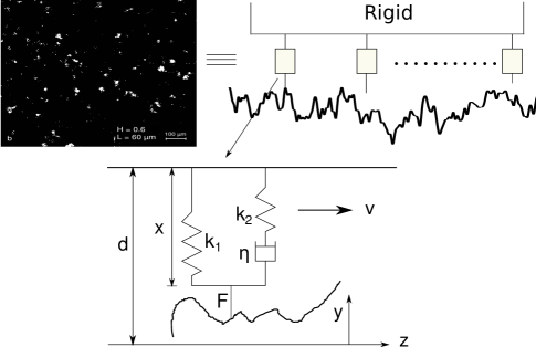
Various theories of contact between surfaces have been proposed. Most surfaces, even those that appear smooth, are rough at the microscale. When two such rough surfaces are pressed against each other, actual contact occurs only at a few spots, at the peaks (asperities) of the surfaces (Figure 1). There is a large body of literature on single asperity contact, starting from the problem of elastic contact between spheres first addressed by Hertz to theories that include plasticity and adhesion [21, 22, 23].

Two broad classes of models have been proposed to connect the asperity scale to the experimentally observed features of the macroscopic frictional behavior. In one class, the contacts are considered to be plastic, following Bowden and Tabor [24] who suggested that, because of surface roughness, the actual area of contact is only a small fraction of the nominal area, and high local stresses often reach the yield stresses of the materials. They estimated the coefficient of friction as the ratio of shear strength of contacts to the indentation hardness of the material:

$$F_{N}=A_{r}\sigma_{c},\quad F_{S}=A_{r}\tau_{c},\quad\mu=F_{S}/F_{N}=\tau_{c}/\sigma_{c},$$

where $F_{N}$ and $F_{S}$ are the macroscopic normal and shear loads, $A_{r}$ is the real area of contact, $\sigma_{c}$ is the indentation hardness, $\tau_{c}$ is the asperity shear strength, and $\mu$ is the friction coefficient. Several subsequent studies have incorporated the time and velocity dependence into that framework by representing the shear force at a contact as the product of the contact shear strength that depends on the sliding velocity and area that depends on the age of the contact [25, 26, 27, 28, 29]. The velocity dependence of the shear strength is attributed to an Arrhenius type activation mechanism while the time dependence of the area results from the creep behavior of the material. The proposed formulations have been able to match various friction observations. In these models, it is assumed that each contact has the same shear and normal force per unit area and the evolution of the contact population is accounted for only by the evolution of the total contact area. As the total contact area changes, the normal force per unit area adjusts, providing the only interaction between the macroscale and the single asperity. Hence this class of models is dominated by the behavior of single asperities and does not include the effects of the statistical properties of the contacting rough surfaces.

In the other class of models, the contacts are considered to be elastic. Since the shear and normal forces are no longer proportional at the microscale for this case, the collective behavior of asperities becomes paramount in explaining the proportionality at the macroscale. Archard [30] proposed a hierarchical model in which each elastic contact is made of multiple contacts at a smaller scale. This is a precursor to the fractal models of contact [31, 32, 33]. In the model proposed by Greenwood and Williamson (GW) [34], each asperity is assumed to be spherical and a single contact is modeled according to Hertzian theory. This is fitted within a statistical description of the rough surface. These models are capable of explaining the basic observations of proportionality between the shear and normal forces at the macroscale and hence the constant static coefficient. They ignore however, the spatial features of surface roughness and time-dependent behavior of single asperities. Thus they are unable to explain any evolution of the friction coefficient.

Our study is the first step towards bridging the gap between the two classes of models and examining the interaction between time-dependent behavior of single asperities and statistical properties of the rough contacting surfaces. When two surfaces are held in static contact or slid against each other, the population of contacts evolves: contacts grow, become smaller, and come into and go out of existence. Concomitantly, the forces on the asperities also evolve, not only because of the time dependence of each contact, but also because of the statistical properties of the rough contacting surfaces. This evolution at the microscale results in the evolution of friction, normal force, area of contact etc., at the macroscale. To explore the interaction between these two influences, we represent the system of two surfaces in contact by an ensemble of one-dimensional viscoelastic elements in contact with a rough rigid surface. Combining the ideas of the two classes of models, we assume that the local shear force between a contacting element and the rough surface depends both on the sliding velocity and the local normal force. The state of the system at any instant is described by a probability distribution of normal forces experienced by the elements in the ensemble. Any macroscopic variable can be determined by integrating the appropriate quantity with respect to this probability distribution. The global normal force, which is the sum of the normal forces on all contacts, is the first moment with respect to the probability distribution. The macroscopic friction is obtained as an appropriate moment (depending on the local friction law) of the normal force distribution. Therefore, the time, velocity, and history dependence of frictional properties at the macroscale are a manifestation of the evolution of the probability density. Consequently, the behavior at the macroscale can be very different from the behavior of single asperities at the microscale. For example, even if individual asperities have velocity-strengthening local friction (higher resistance when sliding faster), the macroscale behavior can be velocity weakening (lower resistance when sliding faster).

We describe our multiscale model for friction, discuss its properties, and compare its results with experiments in Section 3. We also compare our results to commonly used rate and state phenomenological laws, and propose a new interpretation for the state variable that enters the laws. In Section 4, we summarize our findings and suggest ways in which the model can be improved.

2 Background

2.1 Static friction coefficient

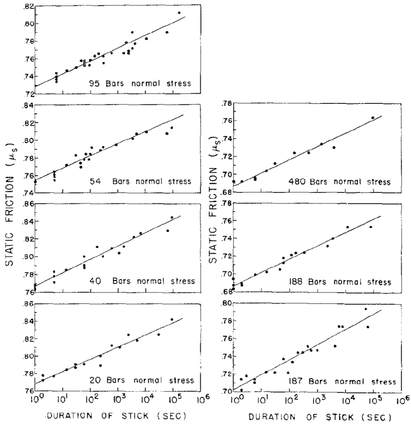
Coulomb observed that the static friction coefficient $\mu_{s}$ is not a constant but depends on how long surfaces are in contact before sliding begins [35]. He proposed an empirical power law to fit his experimental results. Rabinowicz [13] and Dieterich [36] observed a similar strengthening in their experiments on metals and rocks respectively. In Dieterich’s experiments [36], rocks were held at constant normal and shear forces for varying lengths of time before the shear force was suddenly increased to induce sliding. The coefficient of static friction was calculated as the ratio of the shear force required to initiate sliding to the applied normal force. $\mu_{s}$ was observed to increase logarithmically with the time of contact (Figure 2(a)). Dieterich proposed an empirical law to fit these results [14]:

$$\mu_{s}(t)=\mu_{0}+A\log(Bt+1),$$ (1)

where $t$ is the time of stationary contact, $\mu_{0},A$, and $B$ are constants dependent on the two surfaces across the interface. Typically, for rocks, $\mu_{0}$ is $0.7$-$0.8$, $A$ is $0.01$-$0.02$ and $B$ is of the order of $1$ second^-1 [14].

Two physical processes are conjectured to be the origin of the strengthening. First, because of high stresses, creep at contacts might result in increased area of contact, leading to increased strength [37]. Second, even if the area of contact does not change, the strength of each contact might increase with time [24].

(a)

(b)

Figure 2: (a) Evolution of the static friction coefficient with time at a constant normal force for quartz sandstone. Different panels correspond to different values of the normal force. Reproduced with permission from [36]. (b) Evolution of kinetic friction coefficient in velocity jump experiments on different materials. Reproduced with permission from [37].

2.2 Kinetic friction coefficient

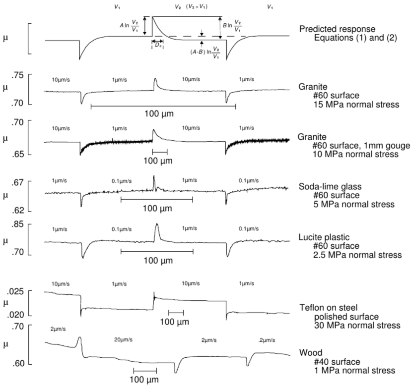
Experiments have shown that the kinetic friction coefficient $\mu_{k}$ depends on the sliding velocity. In a common type of experiments called velocity jump tests, two surfaces are slid at a constant velocity till the system reaches steady state. Then, a step change in sliding velocity is induced and the shear force required to sustain this new velocity is monitored. Since the velocity is constant, by equilibrium, this force must equal the frictional force at the interface. This shear force divided by the applied normal force is the kinetic friction coefficient. Experiments on different materials show [37] that, with a jump in velocity, $\mu_{k}$ also jumps (called direct effect), and the jump is followed by an evolution to a new steady state corresponding to the new sliding velocity (Figure 2(b)). The evolution happens over a characteristic length scale, with the time scale of evolution to steady state being the ratio of the length scale to the sliding speed. This length scale, thought to be the slip necessary for the memory of the contacts to fade, is fairly independent of the sliding speed and the normal force but depends on the surface features [38]. Similar properties of the kinetic friction coefficient have been found for sliding of thin granular layers [11].

2.3 Phenomenological laws

A class of empirical laws called “rate and state” (RS) laws has been proposed to capture the above experimental observations [38, 17]. “Rate” here refers to the relative speed across the interface and “state” refers to one or more internal variables used to represent the memory in the system. These laws, used widely in simulations of earthquake phenomena, have been successful in reproducing many of the observed features of earthquakes [39, 2, 40, 41, 42]. One commonly used RS law with a single state variable takes the form:

$$\mu_{k}=\mu_{0}+a\ln(\frac{v}{v^{*}})+b\ln(\frac{v^{*}\theta}{D_{c}}),$$ (2)

where $\mu_{k}$ is the coefficient of friction, $v$ is the sliding velocity, $a,b,v^{*},\mu_{0}$, and $D_{c}$ are constants, and $\theta$ is an internal variable with dimensions of time. An evolution law is prescribed for the internal variable $\theta$. Two well-known laws are the aging law,

$$\dot{\theta}=1-\frac{v\theta}{D_{c}},$$ (3)

and the slip law,

$$\dot{\theta}=-\frac{v\theta}{D_{c}}\ln(\frac{v\theta}{D_{c}}).$$ (4)

In these equations, $D_{c}$ is the characteristic length scale over which the coefficient of friction evolves to its steady state in the jump test. $D_{c}$ is related to the roughness of the sliding surfaces and is of the order of microns for most engineering surfaces [38, 43]. At steady state, $\dot{\theta}=0$, and from Equation (3) or (4), $\theta_{ss}(v)=D_{c}/v$. Using this in Equation (2), the steady state friction coefficient is given by,

$$\mu_{ss}(v)=const+(a-b)\ln(\frac{v}{v^{*}}).$$ (5)

If $a-b>0$, the steady state friction coefficient increases with increasing sliding speed and if $a-b<0$, the steady state friction coefficient decreases with increasing sliding speed. The two cases are known as velocity-strengthening and velocity-weakening respectively. This has implications, for example for the stability of sliding, a requirement for stick-slip being $a-b<0$ [17, 44].

3 Collective behavior of viscoelastic asperities

3.1 Basic elements

The basic ingredients of our model are a constitutive description of single asperities at the microscale, and a stochastic characterization of rough surfaces. We now describe these in detail.

3.1.1 Single asperity

The behavior of an asperity depends on various factors such as material properties, local stresses, sliding speed etc. As a first step, we model asperities as being viscoelastic, using a spring-dashpot system known as a Standard Linear Solid (SLS, see Figure 1). An SLS consists of a spring in parallel with a spring and dashpot in series. The equation for the evolution of the force $F$ on an SLS as a function of its length and the rate of change of its length is:

$$\dot{F}=(k_{1}+k_{2})\dot{x}-\frac{k_{2}}{\eta}F+\frac{k_{1}k_{2}}{\eta}(x-x^{0}),$$ (6)

where $k_{1},k_{2}$ are the stiffnesses of springs 1 and 2 respectively, $\eta$ is the viscosity of the dashpot, $x,x^{0}$ are the current and undeformed lengths of spring 1 and dot denotes the time derivative. An asperity can be in two states, in contact or out of contact with the surface it slides on. When in contact, its length evolution is known and the force evolution can be calculated using Equation (6). When out of contact, the force on the asperity is zero and, setting $F=0$ and $\dot{F}=0$ in the Equation (6), the evolution of its length is given by:

$$\dot{x}=-\frac{k_{1}k_{2}}{\eta(k_{1}+k_{2})}(x-x^{0}).$$ (7)

A natural question to ask is whether we can relate the material and geometric properties of the asperities to the parameters $k_{1},k_{2}$ and $\eta$ of the SLS. One way to do this would be to solve a viscoelastic Hertzian problem. Assuming that the asperity is spherical and the material is linear viscoelastic, from the solution of the elastic Hertzian problem, the viscoelastic Hertzian problem can be solved using the method of Laplace transforms [45]. The contact, initially at zero force and deformation, is instantaneously brought to a deformation $\delta_{0}$ and the evolution of the force is computed. The instantaneous force is related to the instantaneous stiffness of the SLS, $k_{1}+k_{2}$, the steady state force is related to $k_{1}$, and the rate of relaxation to steady state is related to $\eta$. The Hertzian contact problem is nonlinear whereas the SLS element is linear. The nonlinearity of the Hertzian problem manifests as the dependence of $k_{1},k_{2}$, and $\eta$ on the deformation $\delta_{0}$. We can however, get an order-of-magnitude estimate of the values of the parameters in our model. Results from such calculations for two materials, Polyvinyl Alcohol (PVOH) and Polystyrene [45], are given below.

PVOH:

$$\frac{k_{1}}{\sqrt{\rho\delta_{0}}}=0.18\text{ GPa},\frac{k_{2}}{\sqrt{\rho\delta_{0}}}=0.15\text{ GPa},\frac{\eta}{\sqrt{\rho\delta_{0}}}=0.48\text{ GPa-s}.$$

Polystyrene:

$$\frac{k_{1}}{\sqrt{\rho\delta_{0}}}=2.75\text{ GPa},\frac{k_{2}}{\sqrt{\rho\delta_{0}}}=0.39\text{ GPa},\frac{\eta}{\sqrt{\rho\delta_{0}}}=4.51\text{ GPa-s}.$$

Above, $\rho$ is the radius of curvature of the asperity.

3.1.2 Rough surfaces

Rough surfaces have been characterized by representing the heights from a reference level as a stochastic process [46, 47]. This characterization has been used extensively in exploring various aspects of contact between surfaces [34, 48, 49]. Profile measurements have shown that many types of surfaces can be modeled as a Gaussian noise with an exponential correlation [50]. Such a noise, known as an Ornstein-Uhlenbeck process, satisfies the following stochastic differential equation:

$$\frac{dy}{dz}=-\frac{1}{\lambda}y(z)+\sqrt{\frac{2}{\lambda}}\sigma\zeta(z).$$ (8)

Here, $y$ is the height of the surface from a reference level (chosen such that the mean height is zero), $z$ is the horizontal spatial variable, $\lambda$ is the correlation length, $\sigma$ is the rms-roughness of the surface and $\zeta(z)$ is a Gaussian white noise with unit standard deviation. For typical surfaces, $\sigma$ and $\lambda$ are of the order of a few microns [50]. We adopt this description of a rough surface. We also assume that the surface is rigid since this considerably simplifies our calculations.

3.1.3 Local friction law

To determine the coefficient of friction, we need the macroscopic normal and shear forces. To compute the macroscopic shear force as a moment with respect to the probability distribution of microscopic normal forces, we need to know how the normal and shear forces are related for a single asperity. We assume local friction laws of the form,

$$s(F,v)=f(v)F+c_{2}F^{n},\quad f(v)=\left\{\begin{array}[]{ll}0&\mbox{$v\leq v_{c}$}\\ \mu_{0}+c_{1}\log(\bar{v})&\mbox{$v>v_{c}$.}\end{array}\right.$$ (9)

$s$ here is the shear force at the contact, $F$ is the local normal force, $v$ is the sliding speed, $\bar{v}$ is the nondimensional sliding speed, $\mu_{0},n,c_{1}$, and $c_{2}$ are constants, $v_{c}$ is the cutoff velocity for the velocity dependence of friction, and $2/3\leq n\leq 1$.

The local friction law depends on the material and geometry of the contacts. If a contact is elastic and its geometry is spherical, then, by the Hertz theory of contact, the area of contact varies as the two-thirds power of the normal force. Further, if the contact has a shear strength $\tau_{max}$, then the local friction law is:

$$A\propto F^{2/3},\qquad s=\tau_{max}A\propto F^{2/3}.$$

As in the Bowden and Tabor model, if contacts are plastic because of the high local stresses, the area of contact is proportional to the normal force and the local friction law is:

$$A\propto F^{1},\qquad s=\tau_{max}A\propto F^{1}.$$

An actual contact may be in between these two limiting cases and thus, the power in the local friction law between $2/3$ and $1$. Also, different contacts in the population may be in different states.

If the surfaces are sliding at a relative speed $v$, the asperities in contact are sheared at a strain rate proportional to the sliding speed, and if the shear resistance depends on the strain rate, then the local friction law will be velocity-dependent. Taking cue from experimental results, we assume this velocity dependence to be logarithmic. A theoretical justification for the logarithmic dependence has been proposed by Rice et al [51].

Alternatively, local friction laws can be derived from theoretical and experimental studies of single asperity contacts. For example, Kogut and Etsion [52] consider the inception of sliding of a single spherical elastoplastic contact and conclude that $\mu\propto F^{-0.345}$ when the normal force by itself does not cause any plastic deformation ($\mu$ here is the single asperity friction coefficient). Note that this is very close to the Hertzian $s\propto F^{2/3}$ approximation above. Archard [53], using a crossed cylinder apparatus, reports $\mu\propto F^{-0.26}$ for perspex and $\mu\propto F^{-1/3}$ for brass. Wandersman et al [9], looking at texture-induced modulations of friction, report that $s\propto F^{0.87}$ for an elastomer on glass.

To summarize, our model for two rough surfaces in contact consists of an ensemble of independent viscoelastic SLS elements sitting on a rigid rough surface modeled as an Ornstein-Uhlenbeck process. With this model, we simulate the static contact and velocity jump experiments to study the time and velocity dependence of friction.

3.2 Static friction

3.2.1 Formulation

In this section, we study the evolution of an ensemble of independent SLS elements in static contact with a rigid rough Gaussian surface (Figure 1) under a global normal force $F_{N}$. The evolution of each SLS is governed by Equations (6) and (7). For simplicity, we assume that the values of $k_{1},k_{2},\eta$ and $x^{0}$ are the same for every element in the ensemble. Without loss of generality, we can set $x^{0}=0$ since this corresponds to choosing a particular reference level to measure the length $x$. Dilatation, which is the distance between the reference planes from which the lengths of the SLS elements $x$ and the heights of the rigid surface $y$ are measured, is denoted by $d$. At any instant $t$ during the evolution of the system, only a fraction of the elements are in contact with the surface and for these, the contact condition implies:

$$x(t)+y=d(t).$$ (10)

Since we have assumed the parameters $k_{1},k_{2},\eta,x^{0}$ to be the same for all the elements in the ensemble, each element can be labeled by the height $y$ of the rigid surface that is sees. At time $t$, the global normal force is given by:

$$F_{N}(t)=\mathbb{E}_{y}(F(t,y))=\int_{d(t)}^{\infty}F(t,y)P_{y}(y)\mathrm{d}y,$$ (11)

where $F(t,y)$ is the force on an SLS corresponding to time $t$ and height $y$ of the rough surface, and $P_{y}(y)$ is the probability distribution of heights of the rough surface. The limits of integration are from $d(t)$ to $\infty$ since elements are in contact with the surface only if the height $y$ is greater than $d(t)$ (since $x^{0}=0$). For a Gaussian distribution of surface heights, we have,

$$P_{y}(y)=\frac{1}{\sqrt{2\pi}\sigma}e^{-\frac{y^{2}}{2\sigma^{2}}},$$ (12)

where $\sigma$ is the rms-roughness of the surface. The elements being viscoelastic, the force in the ones in contact would decrease with time if the dilatation were constant. To reproduce experimental conditions, we constrain the total normal force to be constant. To satisfy this constraint, dilatation has to decrease with time. Differentiating Equation (11) with respect to time gives:

$$\dot{F}_{N}(t)=\int_{d(t)}^{\infty}\frac{\partial{F}}{\partial{t}}(t,y)P_{y}(y)\mathrm{d}y-F(t,d)P_{y}(d)\dot{d}(t).$$ (13)

$F(t,d)=0$ since $y=d(t)$ implies that the contact is formed at time $t$. The evolution equation for the force on an SLS (Equation (6) with $\dot{x}=\dot{d}$; $\dot{y}=0$ as the surface is rigid) gives:

$$\frac{\partial{F}}{\partial{t}}(t,y)=(k_{1}+k_{2})\dot{d}(t)-\frac{k_{2}}{\eta}F(t,y)+\frac{k_{1}k_{2}}{\eta}(d(t)-y).$$ (14)

Using $F(t,d)=0$ and Equation (14) in Equation (13), the evolution equation for the dilatation at constant normal force ($\dot{F}_{N}=0$) is:

$$\dot{d}(t)=\frac{\frac{k_{2}}{\eta}F_{N}-\frac{k_{1}k_{2}}{\eta}\int_{d(t)}^{\infty}(d(t)-y)P_{y}(y)\mathrm{d}y}{(k_{1}+k_{2})\int_{d(t)}^{\infty}P_{y}(y)\mathrm{d}y}.$$ (15)

We now turn to the static friction force. Knowing the local friction law, $s=s(F)$, we can determine the global shear force as,

$$F_{S}(t)=\mathbb{E}_{y}(s(F(t,y)))=\int_{d(t)}^{\infty}s(F(t,y))P_{y}(y)\mathrm{d}y,$$ (16)

and the coefficient of friction can be calculated as the ratio of the two forces,

$$\mu_{s}(t)=\frac{F_{S}(t)}{F_{N}}.$$ (17)

Before proceeding further, we nondimensionalize the equations.

3.2.2 Nondimensionalization

To nondimensionalize time, we use $\eta/k_{2}$, which is one of the two characteristic timescales of the SLS. A natural length scale in the problem is the rms-roughness of the surface, $\sigma$. For forces, we use $k_{1}\sigma$. Using these characteristic quantities, we define the following nondimensional variables:

$$\bar{t}=\frac{t}{\eta/k_{2}},\quad\bar{d}=\frac{d}{\sigma},\quad\bar{y}=\frac{y}{\sigma},\quad\bar{F}=\frac{F}{k_{1}\sigma}.$$ (18)

Equation (14) after nondimensionalization is:

$$\frac{\partial{\bar{F}}}{\partial{\bar{t}}}(\bar{t},\bar{y})=R\bar{d}^{\prime}-\bar{F}(\bar{t},\bar{y})+\bar{d}(\bar{t})-\bar{y}.$$ (19)

The nondimensional equation for the dilatation evolution is:

$$\bar{d}^{\prime}=\frac{\bar{F}_{N}(\bar{t})-\int_{\bar{d}}^{\infty}(\bar{d}-\bar{y})P_{\bar{y}}(\bar{y})\mathrm{d}\bar{y}}{R\int_{\bar{d}}^{\infty}P_{\bar{y}}(\bar{y})\mathrm{d}\bar{y}},$$ (20)

and the coefficient of friction is given by:

$$\mu_{s}(\bar{t})=\frac{\bar{F}_{S}(\bar{t})}{\bar{F}_{N}}.$$

In the above equations, prime denotes differentiation with respect to nondimensionalized time,

$$R=1+\frac{k_{2}}{k_{1}},$$ (21)

and the probability distribution of the normalized surface heights $P_{\bar{y}}(\bar{y})=\frac{1}{\sqrt{2\pi}}e^{-\frac{\bar{y}^{2}}{2}}$.

After nondimensionalization, we have two parameters: $R$, which is the ratio between the instantaneous and steady state stiffnesses, and $n$, the power in the local friction law. The local friction exponent $n$ is indicative of the state of the contact, being $2/3$ for elastic and $1$ for plastic contact.

3.2.3 Static friction evolution

Suppose that, at $t=0$, an ensemble of SLS elements is instantaneously brought to a dilatation $d=d_{0}$ against the rigid surface. Some of the SLS elements come into contact with the surface and result in a total normal force $F_{N}$. The system is then allowed to evolve at this constant global normal force $F_{N}$. The dilatation evolves to satisfy the constraint of constant $F_{N}$. This evolution can be calculated using Equation (20). From the dilatation history, the evolution of the probability density of the normal forces can be determined using Equation (19). Using this and the local friction law, we can determine the evolution of the static friction coefficient.

Figure 3 shows the evolution of $\mu_{s}$ for different local friction exponents. At small times, $\frac{t}{\eta/k_{2}}\ll 1$, $\mu_{s}$ remains constant since the SLS elements need a finite time to start relaxing. $\mu_{s}$ then starts increasing and, around the relaxation time of the SLS, $\frac{t}{\eta/k_{2}}=\mathcal{O}(1)$, the increase is approximately logarithmic in time. At large times, $\frac{t}{\eta/k_{2}}\gg 1$, all the SLS elements have relaxed to their steady state and $\mu_{s}$ evolves to a constant value.

Figure 3: Evolution of the static friction coefficient ($\mu_{s}$) with time at a constant global normal force for different local friction exponents $n$. For the physically relevant values of $n\in[2/3,1)$, $\mu_{s}$ increases logarithmically with time for a range of times around the relaxation time of each asperity. For the unphysical case $n>1$, $\mu_{s}$ decreases with time, a behavior that has not been observed in experiments.

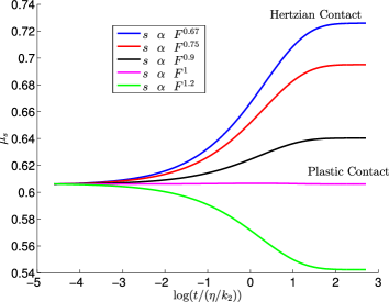
The variation in $\mu_{s}$ is largest for the case of elastic contacts ($n=2/3$). As the power in the local friction law reaches $1$, the case of plastic contacts, we recover the result of the Bowden and Tabor model in which the friction coefficient is a constant given by the ratio of the shear strength to the hardness of the contacts. For $n>1$, $\mu_{s}$ decreases with the time of contact. As explained in section 3.1.3, we expect $n\in[2/3,1]$ for real materials. We believe this to be the reason why we only see an increase of $\mu_{s}$ in experiments.

(a)

(b)

Figure 4: (a) Evolution of friction coefficient with time at a constant global normal force for different stiffness ratios, $R=1+k_{2}/k_{1}$. The system reaches steady state faster for smaller $R$. (b) The saturation at small and large times has also been observed in some experiments (reproduced with permission from [54]).

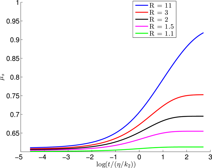
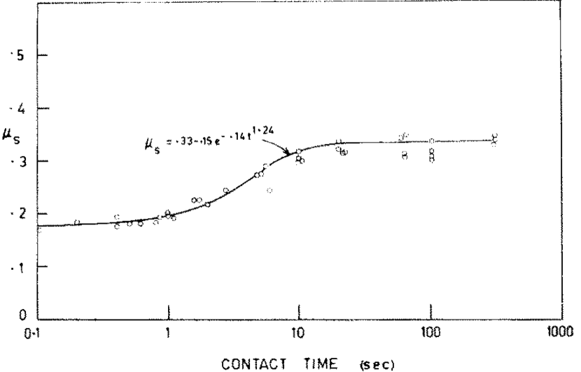
Figure 4(a) shows the evolution of $\mu_{s}$ for different values of $R$, using a local friction law $s(F)\propto F^{0.75}$. When $R\approx 1$, or $k_{2}\ll k_{1}$, the instantaneous and steady state stiffnesses are not very different and hence, the growth in the friction coefficient is small. For $k_{2}\gg k_{1}$, the instantaneous and steady state stiffnesses are very different and consequently, we see a larger growth in $\mu_{s}$. Also, Figure 4(a) shows that the steady state is reached faster when $R$ is smaller. The SLS has two characteristic timescales, $\eta/k_{2}$ and $\frac{\eta}{k_{2}}(1+k_{2}/k_{1})$. Since we have nondimensionalized time with $\eta/k_{2}$, $R$ is the second characteristic timescale in nondimensionalized time and thus, for smaller $R$, the steady state is achieved faster.

The predicted increase of the coefficient of static friction with time has been widely observed in experiments [13, 36, 54]. If $\eta/k_{2}$ is of $\mathcal{O}(1)$ seconds, as it is for the two materials mentioned earlier, we see that the friction coefficient reaches its steady state at around $10^{2}$ seconds and the total variation in $\mu_{s}$ lasts about $3$-$4$ decades in time. In some materials like mild steel, the predicted behavior – linear increase with logarithmic time over a few decades with a lower and upper saturation for small and large times – is also in agreement with experimental observations [55, 54], as shown in the Figure 4(b). In the experiments on rocks [36, 14] however, the logarithmic growth persists through the duration of the experiment (some experiments have lasted six decades in time). Since $\mu_{s}$ cannot increase indefinitely, it eventually has to reach a steady state. This delayed saturation is not captured by our model. We conjecture that the difference between our model response and the rock experiments could be for the following reasons. The SLS element has only one relaxation time, while a real viscoelastic material has many relaxation timescales. In Figures 3 and 4(a), the x-axis is the nondimensionalized logarithmic time. When plotted with respect to logarithmic time, changing $\eta/k_{2}$ corresponds to translating the curve horizontally by $\log(\eta/k_{2})$. Thus, in the case of multiple relaxation timescales (multiple $\eta/k_{2}$), the region of $\mu_{s}$ increase will be wider. Furthermore, if the asperities interact with each other through the bulk, the interactions can result in a continuum of timescales for the response at the macroscopic scale. Exploring this hypothesis remains a topic of current work.

3.3 Kinetic friction

3.3.1 Formulation

Consider a single SLS sliding on a rough rigid surface (Figure 1). The slider can be in two states, in contact or out of contact with the surface. When in contact, its length evolves to conform to the rigid surface, $x(t)=d(t)-y(t)$ and the force evolves according to Equation (6). Since we have modeled the rough surface as a stochastic process, the differential equation for force evolution during contact will also be a stochastic one. If the SLS ensemble slides at a constant velocity $v$, then the horizontal coordinate is $z=vt$. Using chain rule, we can change the independent variable from the horizontal coordinate $z$ to time $t$ in Equation (8) for the rough surface:

$$\frac{dy}{dt}=\frac{dy}{dz}\frac{dz}{dt}=v\frac{dy}{dz}=-\frac{v}{\lambda}y(t)+\sqrt{\frac{2v}{\lambda}}\sigma\zeta(t).$$ (22)

When the slider is in contact with the surface, $\dot{x}=\dot{d}-\dot{y}$. Using this and Equation (22) in Equation (6), the stochastic differential equation for the evolution of the normal force during contact is:

$$\dot{F}(t)=-\frac{k_{2}}{\eta}F(t)+(k_{1}+k_{2})\dot{d}(t)+\frac{k_{1}k_{2}}{\eta}(d(t)-x^{0})+\left(\frac{(k_{1}+k_{2})v}{\lambda}-\frac{k_{1}k_{2}}{\eta}\right)y(t)-(k_{1}+k_{2})\sqrt{\frac{2v}{\lambda}}\sigma\zeta(t).$$ (23)

Here, the terms $y(t)$ and $\zeta(t)$ are the Ornstein-Uhlenbeck and white noise, respectively. Their statistical properties are:

$$<y(t)>=0,\qquad<y(t_{1})y(t_{2})>=\sigma^{2}e^{-\frac{v|t_{1}-t_{2}|}{\lambda}},$$ (24)

$$<\zeta(t)>=0,\qquad<\zeta(t_{1})\zeta(t_{2})>=\delta(t_{1}-t_{2}),$$

$$<\zeta(t_{1})y(t_{2})>=\begin{cases}0,&\mbox{if }t_{1}>t_{2},\\ \sqrt{\frac{2v}{\lambda}}\sigma e^{-v|t_{2}-t_{1}|/\lambda},&\mbox{if }t_{1}<=t_{2},\end{cases}$$

where $<>$ denotes ensemble average. Since $y(t)$ is driven by $\zeta(t)$ (Equation (22)), the cross correlation between the two noises is not zero.

When the slider is not in contact, the normal force is zero and its length evolves according to Equation (7). Before proceeding further, we nondimensionalize the above system of equations.

3.3.2 Nondimensionalization

As before, we use $\sigma$ to nondimensionalize length, $\eta/k_{2}$ to nondimensionalize time and $k_{1}\sigma$ to nondimensionalize force, and use a bar to denote non-dimensional quantities. Equation (23) for an SLS in contact, after nondimensionalization is:

$$\bar{F}^{\prime}=-\bar{F}+R\bar{d}^{\prime}+\bar{d}-\bar{x^{0}}+\left(\frac{R\bar{v}}{\bar{\lambda}}-1\right)\bar{y}-R\sqrt{\frac{2\bar{v}}{\bar{\lambda}}}\bar{\zeta},$$ (25)

$$<\bar{y}>=0,\quad<\bar{y}(\bar{t}_{1})\bar{y}(\bar{t}_{2})>=e^{-\bar{v}|\bar{t}_{1}-\bar{t}_{2}|/\bar{\lambda}},\\$$ (26)

$$<\bar{\zeta}>=0,\quad<\bar{\zeta}(\bar{t}_{1})\bar{\zeta}(\bar{t}_{2})>=\delta(\bar{t}_{1}-\bar{t}_{2}).$$

After nondimensionalization, Equation (7) for an SLS out of contact becomes:

$$\bar{x}^{\prime}=-\frac{1}{R}(\bar{x}-\bar{x}^{0}).$$ (27)

As before prime denotes differentiation with respect to $\bar{t}$.

$\bar{x}^{0}$, the undeformed length of the viscoelastic sliders, may be set to $0$ since this is equivalent to choosing a reference level. $\bar{\lambda}$ is the correlation length of the surface, which we set to $1$. In the governing equations, $\bar{\lambda}$ appears only as $\bar{v}/\bar{\lambda}$, thus $\bar{\lambda}$ sets a scale for the sliding speed.

This leaves the following non-trivial parameters in the model. $R$, as in the static contact case, is the ratio of the instantaneous and steady state stiffnesses of the SLS. $\bar{v}=k_{2}v/\eta\sigma$, a nondimensional sliding speed, is the number of rms-roughness lengths that the SLS slides in one relaxation time $\eta/k_{2}$. If $\bar{v}\gg 1$, the SLS has little time to relax when in contact and hence its response will be close to its instantaneous elastic response. If $\bar{v}\ll 1$, the SLS has time to relax to its steady state and its response will be similar to its steady state elastic response.

We have four parameters in the local friction law, $\mu_{0},c_{1},c_{2},n$ (Equation 9). $\mu_{0}$ sets a reference value for the coefficient of friction, and we choose this to be $0.6$. The constant $c_{1}$ controls velocity dependence of the local friction and it is set to $0.01$ unless otherwise mentioned. The constant $c_{2}$ describes the evolution of the friction on steady sliding, and it is set to $0.2$. Unless mentioned otherwise, the local friction exponent $n$ is set to $0.67$ since the transient is most pronounced in this case.

3.3.3 From one to many

As the surfaces slide, each asperity sees a different profile. If two asperities are close to each other, the profiles they see will be correlated. We neglect this correlation and associate an independent realization of the noise $\bar{y}(\bar{t})$ as the profile on which an SLS element slides. The question we seek to answer is: Given the statistical properties of $\bar{y}(\bar{t})$, what are the statistical properties of the force $\bar{F}$? In particular, what is the probability density of force $P(\bar{F})$? A stochastic equation such as Equation (25) is known as a Langevin equation. Averaging this equation over the ensemble of realizations of the noise $\bar{y}(\bar{t})$, one can derive a partial differential equation for the evolution of the probability density $P(\bar{t},\bar{F})$ [56]. An example of this is the heat equation which results from the averaging of the stochastic equation corresponding to the Brownian motion of a single particle. We would like to do a similar ensemble averaging of Equation (25). The problem, however, is that we have two sources of noise, $\bar{y}(\bar{t})$ and $\bar{\zeta}(\bar{t})$, and the two are correlated (Equation (24)). In such a case, there is no known method of deriving the partial differential equation for the evolution of probability density. Hence, we resort to a numerical Monte Carlo method where we generate an ensemble of sliders and surface profile realizations, evolve the system at the microscale, and compute statistics of the ensemble to determine macroscopic properties. There is however, a particular case of pure white noise, where we can derive a partial differential equation for the evolution of $P(\bar{t},\bar{F})$.

3.3.4 The case of pure white noise

In Equation (25), if the velocity $\bar{v}=\bar{\lambda}/R$, the coefficient of $\bar{y}$ becomes zero. We are then left with only the white noise term and we can derive a partial differential equation (Fokker-Planck equation) for the evolution of $P(\bar{t},F)$ . The Fokker-Planck equation corresponding to the Langevin equation (25) when $\bar{v}=\bar{\lambda}/R$ is [56]:

$$\frac{\partial{P}}{\partial{\bar{t}}}+\frac{\partial{S}}{\partial{\bar{F}}}=0,$$ (28)

$$S(\bar{t},\bar{F})=\left[-\bar{F}+R\bar{d}^{\prime}+\bar{d}-\bar{x^{0}}-R\frac{\partial}{\partial{\bar{F}}}\right]P(\bar{t},\bar{F}).$$ (29)

Here, $S(\bar{t},\bar{F})$ is the flux of $P(\bar{t},\bar{F})$. To complete the problem, we need boundary conditions at $\bar{F}=0$ and $\bar{F}=-\infty$ $\left(\bar{F}\in(-\infty,0]\text{, no tension at contacts}\right)$. At $\bar{F}=-\infty$, both the probability density and flux have to vanish. The boundary condition at $\bar{F}=0$ is nontrivial. The flux there depends on the sliders coming into and going out of contact, since this corresponds to the force changing between zero and nonzero values. We know of no way of explicitly deriving this boundary condition.

Let us look at the steady state. At steady state, $\frac{\partial{P}}{\partial{\bar{t}}}=0$ and $\bar{d}^{\prime}=0$. From Equation (28), the flux is uniform in the domain and $S(-\infty)=0$ implies it is zero everywhere. Setting Equation (29) to zero, the probability density at steady state is:

$$P(\bar{F})=ce^{-\frac{\bar{F}^{2}}{2R}+\frac{(\bar{d}-\bar{x^{0}})\bar{F}}{R}}.$$ (30)

There are two unknowns here, the constant $c$ and the steady state dilatation $\bar{d}$. We have one constraint, that the first moment of the probability density be equal to the applied normal force. Using the constraint, we can relate the constant $c$ and the dilatation $\bar{d}$ as,

$$c=\frac{\bar{F}_{N}}{\int_{\bar{d}}^{\infty}\bar{F}e^{-\frac{\bar{F}^{2}}{2R}+\frac{(\bar{d}-\bar{x^{0}})\bar{F}}{R}}\mathrm{d}\bar{F}}.$$ (31)

The other constraint comes from the boundary condition at $\bar{F}=0$ which cannot be determined explicitly.

3.3.5 Monte Carlo method

Since the Fokker-Planck equation can be derived only a particular velocity, we resort to Monte Carlo simulation in the general case. We generate an ensemble of sliders, each sliding on an independent realization of the noise $\bar{y}(\bar{t})$ with the given statistical properties of Gaussian height distribution and exponential correlation. Again, we assume the parameters $k_{1},k_{2},\eta,x^{0}$ to be the same for all the sliders. The noise is generated at a finite discretization size and this introduces a low-wavelength cutoff in the surface features. The power spectrum of the Ornstein-Uhlenbeck noise is given by:

$$S(\omega)=\frac{\lambda\sigma^{2}}{\pi}\frac{1}{1+\omega^{2}\lambda^{2}},$$

where $\omega$ is the spatial frequency. The power in frequencies beyond 10 times the inverse correlation length is small. Hence, we discretize the surface to resolve this frequency [57]. For heights of the surface between the discretization points, and the derivative of the surface height, we use spline interpolation.

At $\bar{t}=0$, the ensemble of sliders is brought into contact with the rigid surface and this results in a global normal force $\bar{F}_{N}$. In experiments, the surfaces slide at a constant global normal force. As in the static contact case, the dilatation $\bar{d}$ evolves to satisfy the constant normal force constraint. At each time step, the rate of dilatation is determined to ensure that the global normal force remains constant. Once the rate of dilatation is known, the forces and lengths of all the sliders can be updated. For time stepping, we use a first order Euler method. Since, at any instant, the state of all the sliders and thus the force $\bar{F}$ on each of them is known, we can determine the local shear forces using the local friction law, and, adding them, the global shear force $\bar{F}_{S}$. The friction coefficient is then determined as $\mu_{k}(t)=F_{S}(t)/F_{N}$.

3.3.6 Results

Test of Monte Carlo method:

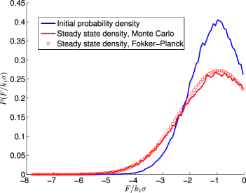
We use the Fokker-Planck equation of Section 3.3.4 as a test of our Monte Carlo method. Starting at an initial state, we let the system slide at the velocity $\bar{v}=\bar{\lambda}/R$ (the case for which we can derive the Fokker-Planck equation) till it reaches steady state. Knowing the normal forces on all the sliders, we can compute the probability density. This density is also known from the solution of the Fokker-Planck equation at steady state (Equations (30) and (31)) and the two can be compared.

Figure 5 shows the probability density of forces in the initial and steady states using the Monte Carlo and Fokker-Planck methods. In this simulation, $R=2,\bar{\lambda}=1$ and thus $\bar{v}=0.5$. An ensemble of $10^{5}$ sliders is used. From the figure, there is a good match in the probability densities using the two methods. As a further verification, we have also computed the transient evolution with the two methods, using the Monte Carlo simulation to prescribe the boundary condition at $\bar{F}=0$ for the Fokker-Planck equation. The two transients also show a good match with each other.

Figure 5: Probability density of normal forces at an initial state, and at steady state using two different methods, a Monte Carlo method and the Fokker-Planck solution.

Velocity jump test:

Drawing confidence from the above result, we perform velocity jump simulations using the Monte Carlo approach. For typical surfaces, $\sigma$ is of the order of a micron and sliding velocities in the jump tests are usually between $0.01\mu$m/s and $100\mu$m/s. $\eta/k_{2}$ is of the order of a few seconds for the two materials mentioned in section 3.1.1. Thus, $\bar{v}$ ranges from $10^{-2}$ to $10^{2}$. Starting from an initial state, we let an ensemble of $10^{5}$ elements slide at $\bar{v}=0.1$ till it reaches steady state. The velocity is then instantaneously changed to $\bar{v}=1$ and the system is allowed to evolve to steady state. Velocity jumps to $\bar{v}=0.1$ and $\bar{v}=1$ are then repeated.

Figure 6(a) shows the evolution of the friction coefficient for two sets of parameter values (all parameters are the same except $R$). In both cases, we find that the friction coefficient changes instantaneously when the velocity jumps, and the change has the same sense as that of the velocity jump; i.e., the friction coefficient jumps up (down) when the velocity jumps up (down). Following the standard rate and state terminology, we call this jump the direct effect. This jump is followed by an evolution towards a steady state. We call this the transient. In both cases, this transient changes the friction coefficient in the direction opposite to the direct effect, i.e., the friction coefficient decreases from the high value following a jump up and increases from a low value following a jump down. In one case ($R=1.1$, or the higher curve), the transient is smaller than the direct effect so that the steady state value is still higher (lower) for an increase (decrease) in velocity. This represents velocity strengthening behavior. In the other case ($R=11$, or the higher curve), the transient is larger than the direct effect so that the steady state value is lower (higher) for an increase (decrease) in velocity. This represents velocity weakening behavior. If the power $n$ in the local friction law is greater than $1$, as shown in Figure 6(b), the friction coefficient change during the transient is in the same direction as the direct effect.

Figure 7 shows the evolution of the dilatation for the same two sets of parameter values. We observe that the dilatation changes continuously with no jumps, and evolves towards a steady state following an imposed velocity jump. Further, the evolution occurs in the same sense, toward higher dilatation for higher velocity and vice versa, for both sets of parameters. The excursions are larger for larger $R$ (the change in dilatation is hardly visible for the case $R=1.1$).

In our model, the force on an asperity changes continuously with time, and therefore the force distribution also changes continuously with time. This is reflected in Figure 7. Therefore, the direct effect in Figure 6(a) is a direct consequence of our local friction law. In fact, the instantaneous increase in $\mu_{k}$ is given by $c_{1}\log(v_{new}/v_{old})$. The subsequent evolution is a result of the collective behavior due to the evolution of the force distribution in addition to the local friction law. Since the dilatation increases with increasing velocity, the applied global normal force is carried by fewer asperities with larger average forces on each (we elaborate on this later). Consequently, if the exponent $n$ in the local friction law satisfies $n<1$ as we expect from the physics, velocity jump will lead to a decrease in friction coefficient during the evolution phase and velocity jump down will lead to an increase in friction coefficient during evolution phase. In short, the direct effect and evolution will always compete with each other.

The above results capture many features of experimental observations. Both the direct effect and the transient are observed in experiments [14, 37, 11]. Further, the direct effect always follows the velocity jump. Furthermore, the direct effect and evolution always change the friction coefficient in opposite directions. This is consistent with the requirement that $n\in[2/3,1]$. Finally, both velocity- strengthening and velocity-weakening behaviors have been observed.

Velocity strengthening vs. velocity weakening:

(a)

(b)

Figure 6: Evolution of friction coefficient in velocity jump tests. (a) For $n<1$, the direct effect and the transient compete against each other. Depending on the parameters, either the instantaneous or the transient effect dominates, leading respectively to velocity strengthening or velocity weakening. (b) For $n>1$, the friction coefficient changes in the same direction during the direct effect and the transient.

Figure 7: Evolution of dilatation in the velocity jump test. The average normal force on an asperity in contact is higher at higher sliding speeds. Thus, for the same global normal force, fewer sliders are in contact at higher speeds and the dilatation is larger. For $R$ close to $1$, the changes in dilatation are hardly apparent.

(a)

(b)

Figure 8: (a) Velocity dependence of the steady-state friction coefficient. Depending on the parameters and the sliding speed, we can have velocity strengthening or velocity weakening. Transitions between strengthening and weakening behaviors have been observed in experiments [58] (b)Probability density of the normal forces at steady state at different sliding speeds (solid lines). At higher speeds, the average normal force on an asperity in contact is higher. Thus, the area under the curve, which represents the fraction of sliders in contact, is smaller at higher speeds. The first moment of the force distribution, which is the global normal force, is the same for all the curves. Also shown is the probability density of forces in a linearized Greenwood-Williamson model with stiffnesses $k_{1}$ and $k_{1}+k_{2}$. These are the force distributions in the limit of $0$ and infinite sliding speeds.

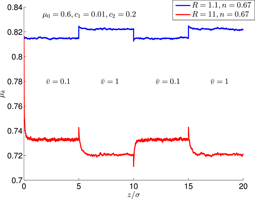
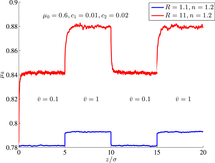
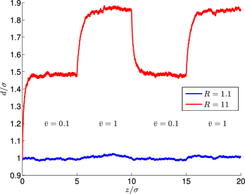
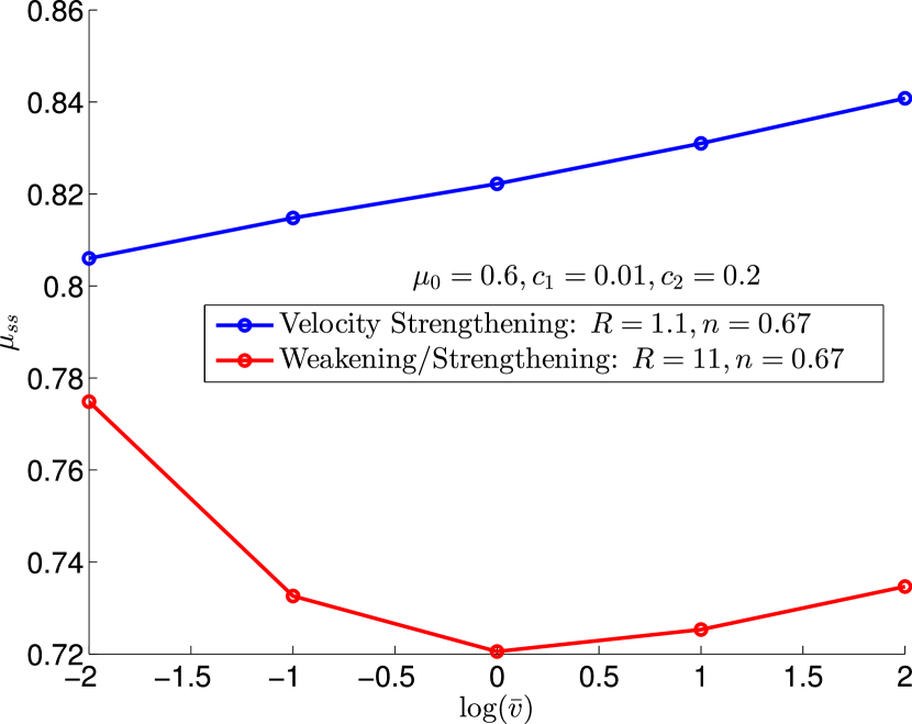
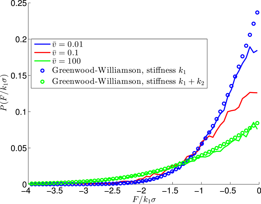
Figure 8(a) shows the dependence of the steady-state friction coefficient on the sliding speed. One case (the blue curve) shows velocity strengthening at all sliding speeds whereas the other case (the red curve) shows velocity weakening at low sliding speeds and strengthening at higher speeds. Since the SLS has only one relaxation timescale, the distribution of forces on asperities is sensitive to the sliding velocity only in a limited range of velocities (the lower velocities for the red curve). Outside this velocity range (the higher velocities for the red curve), the local friction properties dominate and we get velocity-strengthening behavior. The transition between velocity strengthening and velocity weakening has been observed in experiments [58].

Distribution of forces on asperities:

Figure 8(b) shows the probability density of the normal forces at steady state at different sliding speeds. At higher sliding speeds, for the same global normal force, fewer sliders need to be in contact since the normal force on each of the ones in contact is higher on average. This can be seen in the figure where the area under the probability density curve, which represents the fraction of sliders in contact, is smaller at higher speeds. Also shown is the probability density of the normal forces in a linearized version of the Greenwood-Williamson model (where the nonlinear Hertzian contact is replaced by a linear one). The two curves correspond to two different stiffnesses, $k_{1}$ and $k_{1}+k_{2}$. At low sliding speeds, the SLS elements have more time to evolve towards their steady state and thus effectively only the spring with stiffness $k_{1}$ is active during contact. At high speeds, the dashpot has little time to react, and the effective stiffness is nearly $k_{1}+k_{2}$. This can be seen in Figure 8(b) where the probability densities at low and high sliding speeds are similar to the densities of the GW model with stiffnesses $k_{1}$ and $k_{1}+k_{2}$, respectively. The probability densities at different speeds can be mapped to the probability density of the Greenwood-Williamson model with the effective stiffness dependent on the sliding speed.

Characteristic slip distance:

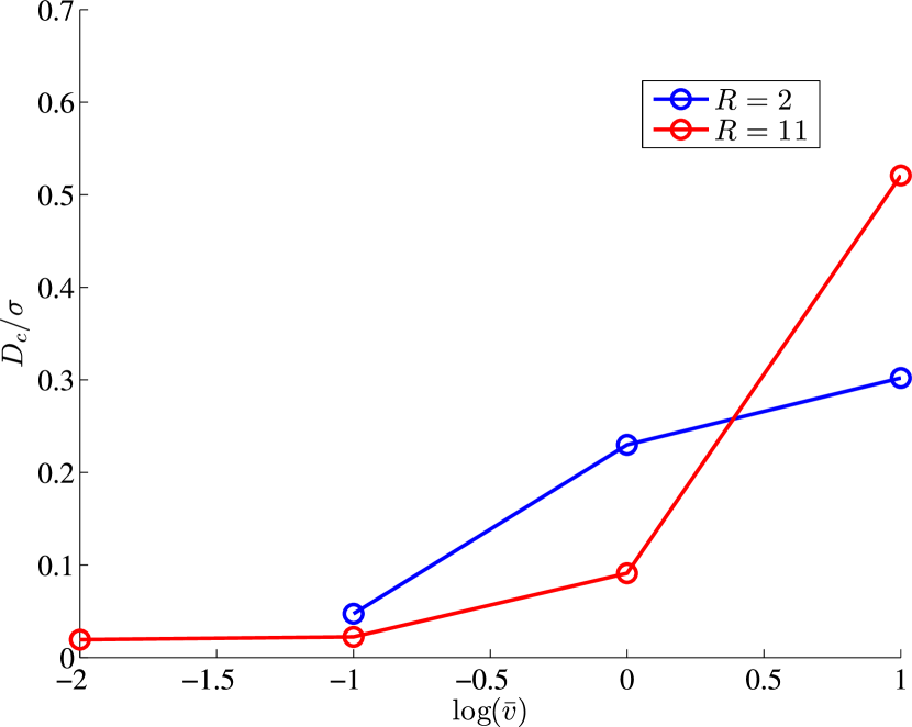
$D_{c}$ is the characteristic length scale over which the system evolves to its steady state in velocity jump tests. We calculate this by fitting an exponential to the evolution of $\mu_{k}$. Figure 9(a) shows the dependence of $D_{c}$ on the sliding speed $\bar{v}$ for two different values of $R$ and for $n=0.67$ and $\bar{\lambda}=1$. $D_{c}$ also depends on the correlation length of the surface, $\bar{\lambda}$. Recall that the parameter $\bar{\lambda}$ appears in the equations only as $\bar{v}/\bar{\lambda}$. If we have two surfaces with correlation lengths $\bar{\lambda}_{1},\bar{\lambda}_{2}$, and the SLS ensemble slides on these surfaces at velocities $\bar{v}_{1}$ and $\bar{v}_{2}$ such that $\bar{v}_{1}/\bar{\lambda}_{1}=\bar{v}_{2}/\bar{\lambda}_{2}$, then the decay lengths are related as:

$$D_{c}(\bar{v}_{1},\bar{\lambda}_{1})=\frac{\bar{\lambda}_{1}}{\bar{\lambda}_{2}}D_{c}(\bar{v}_{2},\bar{\lambda}_{2}).$$

$D_{c}$ is fairly independent of $\bar{v}$ in some laboratory experiments [14], and our simplified model does not capture this independence.

(a)

(b)

Figure 9: (a)The characteristic length over which the system decays to steady state depends on the stiffness ratio $R$ and the sliding speed $\bar{v}$. In many experiments, this distance is found to be a constant that depends only on the roughness of the surfaces. (b)The change in the friction coefficient during the transient phase following the direct effect, for three different combinations of $R$ and $n$. If the change during the transient is greater than the direct effect, we have velocity-strengthening (above the dashed line); otherwise, we have velocity- weakening.

Parametric study:

After nondimensionalization, we have five parameters: $R,\bar{\lambda},n,c_{1}$ and $c_{2}$. Let us study the effect of each of them.

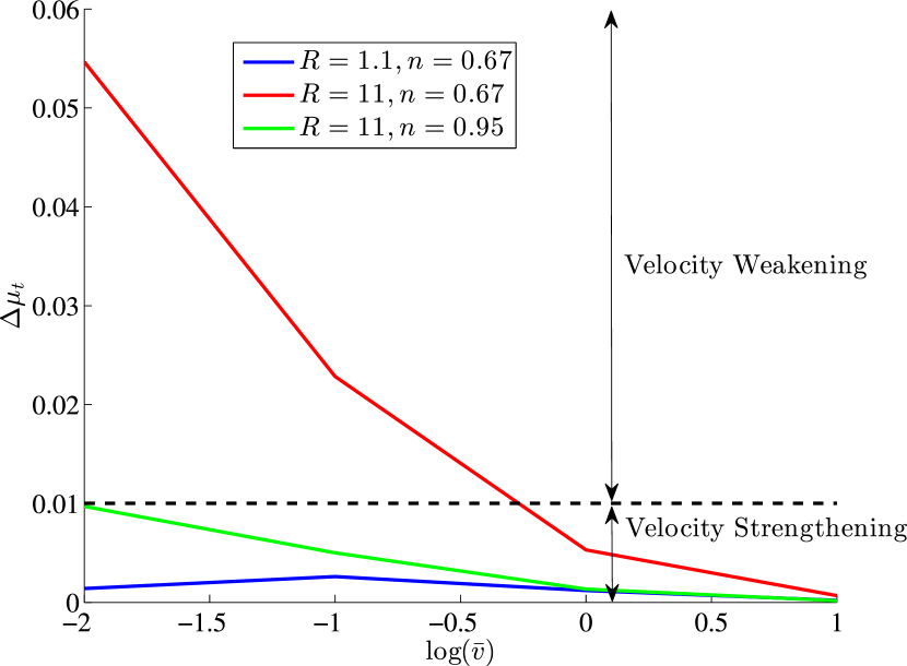
$R=1+k_{2}/k_{1}$ is the ratio between the instantaneous and steady-state stiffnesses of the SLS. When $R$ is close to $1$, the instantaneous and steady-state responses of the SLS are close, the differences between the distribution of forces on asperities at different sliding speeds is small, and thus, the transient change in $\mu_{k}$ following a jump in sliding speed is small. By a similar consideration, for large $R$ $(k_{2}\gg k_{1})$, the transient change in $\mu_{k}$ is large. Hence, for the same instantaneous effect, as the value of $R$ increases, the behavior will change from velocity-strengthening to velocity-weakening, as illustrated in Figure 6(a).

In the governing equations (25), (26), (27), the parameter $\bar{\lambda}$ appears only as $\bar{v}/\bar{\lambda}$. Thus, we can think of $\bar{\lambda}$ as setting a scale for the sliding speed. Consider two surfaces with correlation lengths $\bar{\lambda}_{1}$ and $\bar{\lambda}_{2}$ on which an SLS ensemble slides at two speeds $\bar{v}_{1}$ and $\bar{v}_{2}$. If $\bar{v}_{1}/\bar{\lambda}_{1}=\bar{v}_{2}/\bar{\lambda}_{2}$, and if we start from the same initial state, the evolution of the two systems will be exactly the same. Since we have a velocity dependence in the local friction law, the coefficients of friction of the two systems will differ by $c_{1}\log(\bar{v}_{1}/\bar{v}_{2})$.

The power $n$ in the local friction law represents the elasticity/plasticity of contacts. When $n=1$, all contacts in the ensemble are plastic and the distribution of normal forces among the asperities has no effect on the friction coefficient. This is equivalent to the Bowden and Tabor model, modulo the velocity-dependent term in the local friction law. When $n=2/3$, the effect of distribution of forces among asperities plays an important role in determining $\mu_{k}$. Parameters $c_{1}$ and $c_{2}$ describe the microscopic frictional response of a single contact.

We would like to study how each of the above parameters affects the friction coefficient. To this end, we do velocity jump experiments at different speeds for different values of the parameters $R$ and $n$, and calculate the change in $\mu_{k}$ during the transient phase ($\Delta\mu_{t}$) following the instantaneous jump. Figure 9(b) shows the value of $\Delta\mu_{t}$ at different velocities for three different combinations of parameters $R$ and $n$. A value of $c_{2}=0.2$ has been used ($\Delta\mu_{t}$ changes linearly with $c_{2}$). Also shown as a dashed line is $c_{1}$ which has been assumed to be $0.01$. We have velocity strengthening when $\Delta\mu_{t}<c_{1}$ (below the dashed line) and velocity weakening when $\Delta\mu_{t}>c_{1}$ (above the dashed line). In many experiments, $\Delta\mu_{t}$ is observed to be independent of the sliding speed. In our model, $\Delta\mu_{t}$ is not a constant for given material properties but varies with the sliding velocity.

3.3.7 Comparison with rate and state formulations

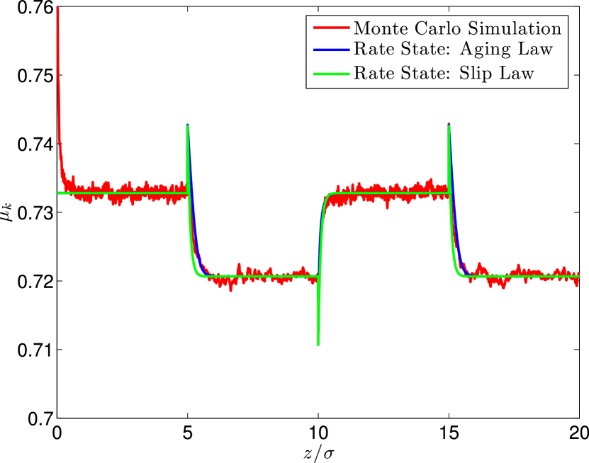
Our results on the evolution of friction coefficient in jump tests can be well fitted by the rate and state equations (2-4), as illustrated in Figure 10(a). In the example shown, the best fit parameters for the rate and state equations are: $\mu_{0}=0.7207,a=0.0043(=c_{1}/\ln 10),b=0.0096$. $v^{*}$ was chosen to be $1$ and $D_{c}/\sigma$ is $0.13$ for the aging law and $0.042$ for the slip law.

(a)

(b)

Figure 10: (a)Evolution of $\mu_{k}$ in a velocity jump test (with $R=11$, $n=0.67$), along with fits for two versions of the rate and state laws. (b)The average time of contact calculated using the Monte Carlo simulation (red), and the evolution of the state variable $\theta$ calculated from the fits in (a). The average time of contact is indeed close to the state variable evolution, supporting the interpretation of the state variable in the rate and state laws as the average contact time.

State variable:

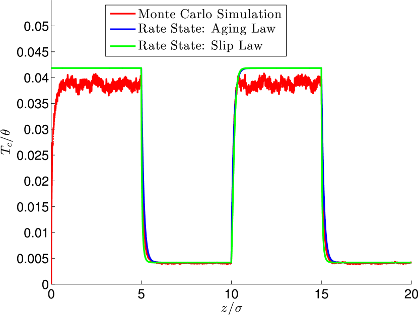
In the rate and state laws, the state variable is sometimes interpreted as the average contact time of the asperities [38, 28]. This time of contact can be calculated explicitly in our simulations. Figure 10(b) shows the evolution of the average time of contact $(T_{c})$ in a velocity jump test. Also shown in the figure is the evolution of the state variable $\theta$ for the two rate and state laws, calculated using the friction evolution fit of Figure 10(a) ($\theta$ does not match $T_{c}$ in absolute value, the figure shows $\theta$ scaled to match $T_{c}$ for the last data point). The steady-state $T_{c}$ is approximately inversely proportional to the sliding speed, as proposed for the state variable in the rate and state formulations. Thus, our model is consistent with the idea that state variable in the rate and state laws is related to the average contact time.

Figure 11: Evolution of the moment of $\bar{F}^{n}$ during the velocity jump test. This moment serves as the state variable in our model.

Moment as a state variable:

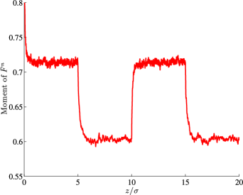
In our model, the transient behavior in the velocity jump tests is proportional to the moment of $\bar{F}^{n}$, i.e., to

$$\psi(\bar{t})=\int_{\bar{F}}\bar{F}^{n}P(\bar{t},\bar{F})\mathrm{d}\bar{F}.$$ (32)

The evolution of this moment is shown in Figure 11 for $n=2/3$. Hence this moment acts as the state variable in our model, and we can formulate the following rate and state description of our model:

$$\mu_{k}(\bar{t})=\mu_{0}+c_{1}\log(\bar{v})+c_{2}\psi(\bar{t}),$$ (33)

$$\psi^{\prime}(\bar{t})=g(\bar{v})(\psi(\bar{t})-\psi_{ss}(\bar{v})),$$ (34)

where $g(\bar{v})$ and $\psi_{ss}(\bar{v})$ can be determined by Monte Carlo simulations for given model parameters $R,n,\bar{\lambda}$. In fact, $g=\bar{v}/\bar{D}_{c}$ where $\bar{D}_{c}$ is shown in Figure 9(a) for $n=0.67$ for two different values of $R$.

3.4 Nonlinear contact model

Until now, we have modeled asperities as linear viscoelastic elements. To test how sensitive the results of our model are to this assumption, we repeat the velocity jump simulations with a modified model for an asperity. We make spring $1$ in the SLS nonlinear. The constitutive equations are:

$$F=k_{1}sgn(x-x^{0})|x-x^{0}|^{3/2}+\eta\dot{x}_{\eta},$$

$$\eta\dot{x}_{\eta}=k_{2}(x_{2}-x_{2}^{0}).$$

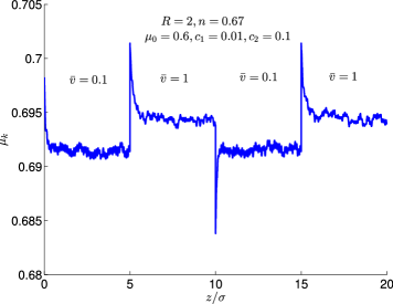
The power $3/2$ has been chosen to mimic Hertzian contact behavior. Using the Monte Carlo method, we repeat the velocity jump experiment. Figure 12 shows that the evolution of the friction coefficient is similar to the linear SLS case. While not conclusive, this example suggests that the qualitative features of the results are not crucially dependent on the particular description of a single asperity.

Figure 12: Velocity jump experiment with a nonlinear asperity model. The evolution of friction coefficient is qualitatively similar to the evolution in Figure 6(a). Though not conclusive, this suggests that the qualitative features of the results are robust with respect to the single asperity model.

3.5 Multiple timescales

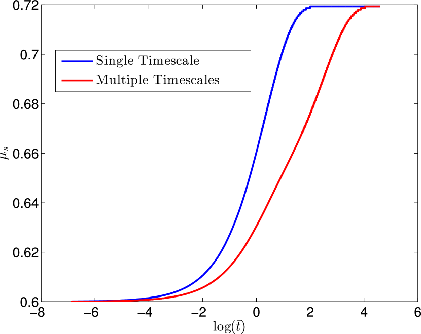
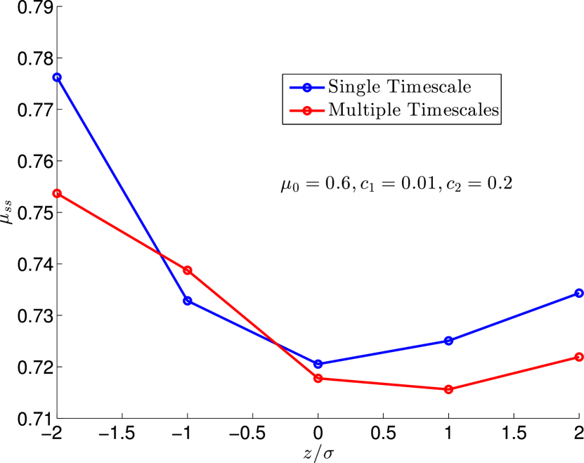
We conjectured that the saturation of the static friction coefficient in $3$-$4$ decades (Figure 3) and the limited velocity range of velocity weakening (Figure 8(a)) is primarily due to the single timescale in the SLS. To verify this, we perform the static contact and velocity jump simulations with an ensemble of SLS having multiple timescales. Figure 13(a) shows the evolution of the static friction coefficient in two cases. In the first case (blue), all sliders in the ensemble have the same relaxation time, $\eta=1$. In the other case (red), half the sliders have $\eta=1$ and the other half have $\eta=10$. The logarithmic growth regime is wider for the case with two timescales. Figure 13(b) shows the steady state friction coefficient as a function of the sliding speed. The first case (blue) has all sliders with $\eta=1$ whereas in the second case (red), half the sliders have $\eta=1$ while the other half have $\eta=0.1$. We see that the case with two timescales has a broader velocity-weakening regime. This confirms our conjecture that the existence of multiple timescales leads to longer evolution of the static friction coefficient and wider velocity-weakening regimes.

(a)

(b)

Figure 13: (a) Evolution of static friction coefficient with hold time for an ensemble of SLS with two timescales. (b) The steady-state friction coefficient as a function of the sliding speed for an ensemble of SLS with two timescales.

4 Conclusion

We have proposed a model for friction between macroscopic surfaces considering asperities at the microscale to be viscoelastic and modeling rough surfaces as a stochastic process. Our main contribution is a framework to link properties of single asperities and surface features to the macroscopic static and sliding frictional behavior. We show that, because of the collective response of contacts, the behavior at the macroscale can be very different from that at the microscale.

Even in our relatively simple model, rate and state effects appear naturally as a consequence of the collective asperity response. The model reproduces the logarithmic strengthening of the static friction with hold time, albeit within a limited range of time scales compared to some experiments. For kinetic friction, the model reproduces many experimental observations. To capture the direct effect of these experiments, we need to endow the microscopic asperity-level friction law with a velocity-strengthening dependence. This does not, however, imply that the macroscopic response is velocity-strengthening. The velocity strengthening of individual contacts and the collective behavior together determine whether the macroscopic response is velocity-strengthening or weakening.

The power $n$ in the local friction law plays a crucial role in the evolution of the friction coefficient. If $n>1$, the static friction coefficient decreases with hold time and the transient evolution of kinetic friction in velocity jump experiments happens in the same sense as the instantaneous change. Since we expect the power $n$ to be less than or equal to $1$, this explains why the above two features are not observed in experiments.

At the same time, the model appears to be too simple to reproduce all experimental observations. In particular, our model results in velocity dependence of the characteristic evolution length scale $D_{c}$ and parameter $b$ that quantifies the transient change in friction in the rate and state equations, whereas these quantities are largely velocity-independent in experimental studies for a range of sliding velocities.

There are a number of ways to improve the model. In the present model, individual asperities are independent, the only interaction between them being through a mean field (dilatation). Long-range elastic interactions through the bulk may, however, play an important role. We have also assumed one of the surfaces to be rigid. While this is reasonable when one of the surfaces is much more deformable than the other, when the two surfaces are similar (with respect to deformability), it will be important to incorporate the non-rigidity, especially during sliding. We have neglected the spatial distribution of asperities and contacts; this will, however, be important for reproducing realistic frictional behavior, especially when the long-range interactions are incorporated. Depending on the material of the sliding surfaces, the model for a single asperity can be modified to incorporate effects such as plasticity, adhesion etc. These issues remain a topic of current and future work.

References

- [1] M. Urbakh, J. Klafter, D. Gourdon, and J. Israelachvili. The nonlinear nature of friction. Nature, 430:525–528, July 2004.
- [2] JH Dieterich. Applications of rate-and state-dependent friction to models of fault slip and earthquake occurrence. Treatise on Geophysics, 4:107–129, 2007.
- [3] H Peter Jost. Tribology - origin and future. Wear, 136(1):1–17, 1990.
- [4] Bharat Bhushan. Principles and applications of tribology. John Wiley & Sons, 2013.
- [5] Nikhil S Tambe and Bharat Bhushan. Scale dependence of micro/nano-friction and adhesion of mems/nems materials, coatings and lubricants. Nanotechnology, 15(11):1561, 2004.
- [6] IR McFadyen, EE Fullerton, and MJ Carey. State-of-the-art magnetic hard disk drives. MRS Bulletin-Materials Research Society, 31(5):379, 2006.
- [7] Bharat Bhushan. Nanotribology and nanomechanics of mems/nems and biomems/bionems materials and devices. Microelectronic Engineering, 84(3):387–412, 2007.
- [8] J Scheibert, S Leurent, A Prevost, and G Debregeas. The role of fingerprints in the coding of tactile information probed with a biomimetic sensor. Science Signalling, 323(5920):1503, 2009.
- [9] E Wandersman, R Candelier, G Debrégeas, and Alexis Prevost. Texture-induced modulations of friction force: the fingerprint effect. Physical review letters, 107(16):164301, 2011.
- [10] C. H. Scholz. Earthquakes and friction laws. Nature, 391(6662):37–42, January 1998.
- [11] C Marone. Laboratory-derived friction laws and their application to seismic faulting. ANNUAL REVIEW OF EARTH AND PLANETARY SCIENCES, 26:643–696, 1998.
- [12] Duncan Dowson and Duncan Dowson. History of tribology. Longman London, 1979.
- [13] Ernest Rabinowicz. Friction and wear of materials, volume 2. Wiley New York, 1965.
- [14] J. H. Dieterich. Time-dependent friction and the mechanics of stick-slip. Pure and Applied Geophysics, 116:790–806, July 1978.
- [15] Christopher H Scholz. The mechanics of earthquakes and faulting. Cambridge university press, 2002.
- [16] N. M. Beeler, T. E. Tullis, and J. D. Weeks. The roles of time and displacement in the evolution effect in rock friction. Geophysical Research Letters, 21:1987–1990, September 1994.
- [17] A. Ruina. Slip instability and state variable friction laws. Journal of Geophysical Research, 881:10359–10370, December 1983.
- [18] Vikas Prakash and Rodney J Clifton. Time resolved dynamic friction measurememts in pressure-shear. ASME APPLIED MECHANICS DIVISION-PUBLICATIONS-AMD, 165:33–33, 1993.
- [19] MF Linker and JH Dieterich. Effects of variable normal stress on rock friction: Observations and constitutive equations. Journal of Geophysical Research: Solid Earth (1978–2012), 97(B4):4923–4940, 1992.
- [20] James H Dieterich and Brian D Kilgore. Imaging surface contacts: power law contact distributions and contact stresses in quartz, calcite, glass and acrylic plastic. Tectonophysics, 256(1):219–239, 1996.
- [21] Bharat Bhushan. Contact mechanics of rough surfaces in tribology: single asperity contact. Applied mechanics reviews, 49:275, 1996.
- [22] KL Johnson, K Kendall, and AD Roberts. Surface energy and the contact of elastic solids. Proceedings of the Royal Society of London. A. Mathematical and Physical Sciences, 324(1558):301–313, 1971.
- [23] BV Derjaguin, VM Muller, and Yu P Toporov. Effect of contact deformations on the adhesion of particles. Journal of Colloid and interface science, 53(2):314–326, 1975.
- [24] Frank Philip Bowden and David Tabor. The friction and lubrication of solids. Clarendon Press, 1986, page 374, 1986.
- [25] Y Brechet and Y Estrin. The effect of strain rate sensitivity on dynamic friction of metals. Scripta metallurgica et materialia, 30(11):1449–1454, 1994.
- [26] Y Estrin and Y Bréchet. On a model of frictional sliding. pure and applied geophysics, 147(4):745–762, 1996.
- [27] P Berthoud, T Baumberger, C G’sell, and J-M Hiver. Physical analysis of the state-and rate-dependent friction law: Static friction. Physical review B, 59(22):14313, 1999.
- [28] T. Baumberger, P. Berthoud, and C. Caroli. Physical analysis of the state- and rate-dependent friction law. ii. dynamic friction. Phys. Rev. B, 60:3928–3939, Aug 1999.
- [29] Thibaut Putelat, Jonathan H.P. Dawes, and John R. Willis. On the microphysical foundations of rate-and-state friction. Journal of the Mechanics and Physics of Solids, 59(5):1062 – 1075, 2011.
- [30] J. F. Archard. Elastic deformation and the laws of friction. Proceedings of the Royal Society of London. Series A. Mathematical and Physical Sciences, 243(1233):190–205, 1957.
- [31] A. Majumdar and B. Bhushan. Fractal model of elastic-plastic contact between rough surfaces. Journal of Tribology, 113(1):1–11, 1991.
- [32] Bo NJ Persson. Theory of rubber friction and contact mechanics. The Journal of Chemical Physics, 115(8):3840–3861, 2001.
- [33] M Ciavarella, G Demelio, JR Barber, and Yong Hoon Jang. Linear elastic contact of the weierstrass profile. Proceedings of the Royal Society of London. Series A: Mathematical, Physical and Engineering Sciences, 456(1994):387–405, 2000.
- [34] J. A. Greenwood and J. B. P. Williamson. Contact of nominally flat surfaces. Proceedings of the Royal Society of London. Series A. Mathematical and Physical Sciences, 295(1442):300–319, 1966.
- [35] B.N.J. Persson. Sliding friction: physical principles and applications. Nanoscience and technology. Springer, 2000.
- [36] J. H. Dieterich. Time-dependent friction in rocks. J. Geophys. Res., 77:3690–97, 1972.
- [37] J. H. Dieterich and B. D. Kilgore. Direct observation of frictional contacts: New insights for state-dependent properties. Pure and Applied Geophysics, 143:283–302, March 1994.
- [38] J. H. Dieterich. Modeling of rock friction 1. Experimental results and constitutive equations. Journal of Geophysical Research, 84:2161–2168, May 1979.
- [39] Simon T Tse and James R Rice. Crustal earthquake instability in relation to the depth variation of frictional slip properties. Journal of Geophysical Research: Solid Earth (1978–2012), 91(B9):9452–9472, 1986.
- [40] Yoshihiro Kaneko, Jean-Philippe Avouac, and Nadia Lapusta. Towards inferring earthquake patterns from geodetic observations of interseismic coupling. Nature Geoscience, 3(5):363–369, 2010.
- [41] Sylvain Barbot, Nadia Lapusta, and Jean-Philippe Avouac. Under the hood of the earthquake machine: toward predictive modeling of the seismic cycle. Science, 336(6082):707–710, 2012.
- [42] Hiroyuki Noda and Nadia Lapusta. Stable creeping fault segments can become destructive as a result of dynamic weakening. Nature, 493(7433):518–521, 2013.
- [43] James H. Dieterich. Constitutive Properties of Faults With Simulated Gouge, pages 103–120. American Geophysical Union, 1981.
- [44] AL Ruina. Stability of steady frictional slipping. Journal of applied mechanics, 50:343–349, 1983.
- [45] L Cheng, X Xia, LE Scriven, and WW Gerberich. Spherical-tip indentation of viscoelastic material. Mechanics of materials, 37(1):213–226, 2005.
- [46] Michael S Longuet-Higgins. The statistical analysis of a random, moving surface. Philosophical Transactions of the Royal Society of London. Series A, Mathematical and Physical Sciences, pages 321–387, 1957.
- [47] Richard S Sayles and Tom R Thomas. Surface topography as a nonstationary random process. 1978.
- [48] P Ranganath Nayak. Random process model of rough surfaces. Journal of Lubrication Technology, 93:398, 1971.
- [49] PR Nayak. Random process model of rough surfaces in plastic contact. Wear, 26(3):305–333, 1973.
- [50] David John Whitehouse and JF Archard. The properties of random surfaces of significance in their contact. Proceedings of the Royal Society of London. A. Mathematical and Physical Sciences, 316(1524):97–121, 1970.
- [51] James R. Rice, Nadia Lapusta, and K. Ranjith. Rate and state dependent friction and the stability of sliding between elastically deformable solids. Journal of the Mechanics and Physics of Solids, 49(9):1865 – 1898, 2001.
- [52] Lior Kogut and Izhak Etsion. A semi-analytical solution for the sliding inception of a spherical contact. Journal of tribology, 125(3):499–506, 2003.
- [53] JF Archard. Single contacts and multiple encounters. Journal of Applied Physics, 32(8):1420–1425, 1961.
- [54] RSH Richardson and H Nolle. Surface friction under time-dependent loads. Wear, 37(1):87–101, 1976.
- [55] JT Oden and JAC Martins. Models and computational methods for dynamic friction phenomena. Computer methods in applied mechanics and engineering, 52(1):527–634, 1985.
- [56] Hannes Risken. The Fokker-Planck equation: Methods of solution and applications, volume 18. Springer Verlag, 1996.
- [57] JA Ogilvy and JR Foster. Rough surfaces: Gaussian or exponential statistics? Journal of Physics D: Applied Physics, 22(9):1243, 1989.
- [58] Toshihiko Shimamoto. Transition between frictional slip and ductile flow for halite shear zones at room temperature. Science, 231(4739):711–714, 1986.