Jacobian fibrations on the singular $K3$ surface of discriminant 3

Abstract.

In this paper we give the Weierstrass equations and the generators of Mordell-Weil groups for Jacobian fibrations on the singular $K3$ surface of discriminant 3.

1. Introduction

A $K3$ surface defined over the complex number field whose Picard number equals to maximum possible number $20$ is called a singular $K3$ surface. Shioda and Inose [10] showed that the map a singular $K3$ surface $X$ corresponds to its transcendental lattice $T_{X}$ is a bijective correspondence from the set of singular $K3$ surfaces onto the set of equivalence classes of positive-definite even integral lattice of rank two with respect to $SL_{2}(\mathbb{Z}$). The discriminant of a singular $K3$ surface $X$ is the determinant of the Gram matrix of the transcendental lattice $T_{X}$.

In this paper we study Jacobian fibrations, i.e., elliptic fibrations with a section, on the singular $K3$ surface $X_{3}$ of discriminant $3$, which corresponds to the lattice defined by $\left(\begin{array}[]{cc}2&1\\ 1&2\end{array}\right)$ and is uniquely determined up to isomorphism. Jacobian fibrations on $X_{3}$ were classified by Nishiyama [8]. He classified all configurations of singular fibers of Jacobian fibrations on $X_{3}$ into $6$ classes and determined their Mordell-Weil groups. Then, we give for each fibration a Weierstrass model. More precisely, we state our main theorem.

Theorem 1.

Let $X_{3}$ be the singular $K3$ surface of discriminant $3$. For each Jacobian fibration in Nishiyama’s list [8, Table 1.1], an elliptic parameter $u_{i}$, a Weierstrass equation and the generators of the Mordell-Weil group are given by Table 1.

No.	sing. fibs	MWG	$u_{i}$	equation and rational points
1	$2\operatorname{II}^{*}+\operatorname{IV}$	$0$	$\frac{2(y_{2}+1)}{(y_{1}-1)^{2}}$	$Y^{2}=X^{3}+u_{1}^{5}(u_{1}-1)^{2}$
				$O$
2	$\operatorname{I}_{12}^{*}+\operatorname{I}_{3}+3\operatorname{I}_{1}$	$\mathbb{Z}/2\mathbb{Z}$	$\frac{2t^{2}}{(y_{2}+1)(y_{1}^{2}+2y_{1}+2y_{2}-1)}$	$Y^{2}=X^{3}-2u_{2}(u_{2}^{3}-2)X^{2}+u_{2}^{8}X$
				$O,\;(0,0)$
3	$\operatorname{III}^{*}+\operatorname{I}_{6}^{*}+3\operatorname{I}_{1}$	$\langle\frac{3}{2}\rangle\oplus\mathbb{Z}/2\mathbb{Z}$	$\frac{t}{y_{1}^{2}-1}$	$Y^{2}=X^{3}+4u_{3}^{3}X^{2}-4u_{3}^{3}X$
				2-tor.: $O,\;(0,0)$
				free gen. : $(1,-1)$
4	$\operatorname{I}_{18}+6\operatorname{I}_{1}$	$\langle\frac{3}{2}\rangle\oplus\mathbb{Z}/3\mathbb{Z}$	$\frac{t}{y_{1}+y_{2}}$	$Y^{2}=X^{3}+(X-u_{4}^{6})^{2}$
				3-tor. : $O,\;(0,\pm u_{4}^{6})$
				free gen. : $(2u_{4}^{3},2u_{4}^{3}+u_{4}^{6})$
5	$3\operatorname{IV}^{*}$	$\mathbb{Z}/3\mathbb{Z}$	$y_{1}$	$Y^{2}=X^{3}+(u_{5}^{2}-1)^{4}$
				$O,\;(0,\pm(u_{5}^{2}-1)^{2}))$
6	$\operatorname{I}_{3}^{*}+\operatorname{I}_{12}+3\operatorname{I}_{1}$	$\mathbb{Z}/4\mathbb{Z}$	$t$	$Y^{2}=X^{3}-2(u_{6}^{3}-2)X^{2}+u_{6}^{6}X$
				$O,\;(0,0),\;(u_{6}^{3},\pm 2u_{6}^{6})$

Table 1. Classification of Jacobian fibrations on $X_{3}$

We explain about Table 1. The fist column shows the name of each Jacobian fibrations following Nishiyama’s notaion. The second column shows the configuration of singular fibers. Here, for example, by $2\operatorname{II}^{*}+\operatorname{IV}$ meanes that the surface has two singular fibers of type $\operatorname{II}^{*}$ and a singular fiber of ot type $\operatorname{IV}$ (Kodaira’s notation [4]). The third column shows the Mordell-Weil group (MWG) of the fibration. The fourth column shows an elliptic parameter $u_{i}$ of the fibration under the singular affine modell (2.6) of $X_{3}$. The index $i$ is the name of the fibration. The last column shows a Weierstrass equation and rational points corresponding to Mordell-Weil generator of the fibration, where $O$ is the rational point corresponding to the zero of MWG.

Recently, Braun, Kimura and Watari [2] showed that Nishiyama’s list also gives the classification of Jacobian fibrations on $X_{3}$ modulo isomorphism. Thus, our and their results answer completely a question of Kuwata and Shioda [7].

2. Notation

The singular $K3$ surface $X_{3}$ is known as a generalized Kummer surface constructed by the following. Let $C_{\omega}$ be the complex elliptic curve with the fundamental periods $1$ and $\omega=e^{2\pi\sqrt{-1}/3}$. Let $\sigma$ be an automorphism of $C_{\omega}\times C_{\omega}$ defined by $\sigma(z_{1},z_{2})\mapsto(\omega z_{1},\omega^{2}z_{2})$. Then the minimal resolution of the quotient $C_{\omega}\times C_{\omega}/\langle\sigma\rangle$ is isomorphic to the singular $K3$ surface $X_{3}$ (see [10, Lemma 5.1]). The automorphism $\sigma$ has the $9$ fixed points $(v_{i},v_{j})\,(1\leq i,j\leq 3)$, where $\{v_{i}\}$ are the fixed points of the automorphism $\sigma_{1}$ of $C_{\omega}$ defined by $\sigma_{1}(z)=\omega z$. These $9$ points $(v_{i},v_{j})$ correspond to the singular points $p_{ij}$ of the quotient $C_{\omega}\times C_{\omega}/\langle\sigma\rangle$. The minimal resolution $X_{3}$ of $C_{\omega}\times C_{\omega}/\langle\sigma\rangle$ is obtained by replacing each $p_{ij}$ by $2$ non-singular rational curves $E_{i,j}$ and $E_{i,j}^{\prime}$ with $E_{i,j}\cdot E_{i,j}^{\prime}=1$. Moreover, $X_{3}$ contains $6$ non-singular rational curves, i.e. the image $F_{i}$ (or $G_{j}$) of $\{v_{i}\}\times C_{\omega}$ (or $C_{\omega}\times\{v_{j}\}$) in $X_{3}$. We have the following intersection numbers.

(2.1) $$F_{i}^{2}=G_{i}^{2}=E_{i,j}^{2}=E_{i,j}^{\prime 2}=-2,\;F_{i}\cdot E_{j,k}=G_{i}\cdot E_{j,k}^{\prime}=F_{i}\cdot G_{j}=0,$$

$$E_{i,j}\cdot E^{\prime}_{k,l}=\delta_{i,k}\cdot\delta_{j,l},\quad F_{i}\cdot E_{j,k}^{\prime}=G_{i}\cdot E_{k,j}=\delta_{i,j}.$$

These $24$ curves on $X_{3}$ form the configuration of Figure 1.

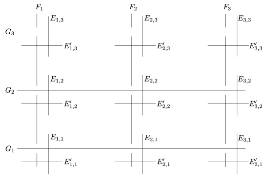
Figure 1. $(-2)$-curves

It is well known that the elliptic curve $C_{\omega}$ has the following Weierstrass form

(2.2) $$C_{\omega}:y^{2}=x^{3}+1.$$

We denote each factor of $C_{\omega}\times C_{\omega}$ by

(2.3) $$C_{\omega}^{1}:y_{1}^{2}=x_{1}^{3}+1,\quad C_{\omega}^{2}:y_{2}^{2}=x_{2}^{3}+1.$$

Then the automorphism $\sigma$ is written by

(2.4) $$\sigma\ : \ C_{\omega}^{1}\times C_{\omega}^{2}\to C_{\omega}^{1}\times C_{\omega}^{2}$$

$$(x_{1},y_{1},x_{2},y_{2})\mapsto(\omega x_{1},y_{1},\omega^{2}x_{2},y_{2}).$$

The function field $\mathbb{C}(X_{3})$ is equal to the invariant subfield of the function field $\mathbb{C}(C_{\omega}^{1}\times C_{\omega}^{2})=\mathbb{C}(x_{1},x_{2},y_{1},y_{2})$ under the automorphism $\sigma$. Then we have

(2.5) $$\mathbb{C}(X_{3})=\mathbb{C}(y_{1},y_{2},t),\quad t=x_{1}x_{2},$$

where $y_{1},y_{2},$ and $t$ are naturally regarded as functions on $X_{3}$ with the relation

(2.6) $$t^{3}=(y_{1}^{2}-1)(y_{2}^{2}-1).$$

This gives a singular affine model of $X_{3}$. We start from the equation to obtain a Weierstrass form for each Jacobian fibration on $X_{3}$. Under the above notation, we see that the divisor of typical functions are as follows.

(2.7) $$\big{(}y_{1}-1\big{)}=3F_{2}+2(E^{\prime}_{2,1}+E^{\prime}_{2,2}+E^{\prime}_{2,3})+E_{2,1}+E_{2,2}+E_{2,3}$$

$$\qquad\qquad\qquad-\left(3F_{1}+2\left(E^{\prime}_{1,1}+E^{\prime}_{1,2}+E^{\prime}_{1,3}\right)+E_{1,1}+E_{1,2}+E_{1,3}\right)$$

$$\big{(}y_{1}+1\big{)}=3F_{3}+2(E^{\prime}_{3,1}+E^{\prime}_{3,2}+E^{\prime}_{3,3})+E_{3,1}+E_{3,2}+E_{3,3}$$

$$\qquad\qquad\qquad-\left(3F_{1}+2\left(E^{\prime}_{1,1}+E^{\prime}_{1,2}+E^{\prime}_{1,3}\right)+E_{1,1}+E_{1,2}+E_{1,3}\right)$$

$$\big{(}y_{2}-1\big{)}=3G_{2}+2(E_{1,2}+E_{2,2}+E_{3,2})+E^{\prime}_{1,2}+E^{\prime}_{2,2}+E^{\prime}_{3,2}$$

$$\qquad\qquad\qquad-\left(3G_{1}+2\left(E_{1,1}+E_{2,1}+E_{3,1}\right)+E^{\prime}_{1,1}+E^{\prime}_{2,1}+E^{\prime}_{3,1}\right)$$

$$\big{(}y_{2}+1\big{)}=3G_{3}+2(E_{1,3}+E_{2,3}+E_{3,3})+E^{\prime}_{1,3}+E^{\prime}_{2,3}+E^{\prime}_{3,3}$$

$$\qquad\qquad\qquad-\left(3G_{1}+2\left(E_{1,1}+E_{2,1}+E_{3,1}\right)+E^{\prime}_{1,1}+E^{\prime}_{2,1}+E^{\prime}_{3,1}\right)$$

$$\big{(}t\big{)}=F_{2}+E^{\prime}_{2,3}+E_{2,3}+G_{3}+E_{3,3}+E^{\prime}_{3,3}+F_{3}+E^{\prime}_{3,2}+E_{3,2}+G_{2}+E_{2,2}+E^{\prime}_{2,2}$$

$$\qquad\qquad-\left(E_{2,1}+E_{3,1}+2\left(G_{1}+E_{1,1}+E^{\prime}_{1,1}+F_{1}\right)+E^{\prime}_{1,2}+E^{\prime}_{1,3}\right).$$

3. Fibration 1

An elliptic parameter for Fibration 1 is given by

(3.1) $$u_{1}=\frac{2(y_{1}+1)}{(y_{1}-1)^{2}}.$$

The divisor of $u_{1}$ is given by

(3.2) $$\left(u_{1}\right) =E^{\prime}_{3,3}+2E_{3,3}+3G_{3}+4E_{1,3}+5E^{\prime}_{1,3}+6F_{1}+3E^{\prime}_{1,1}+4E^{\prime}_{1,2}+2E_{1,2}$$

$$\quad-\left(E^{\prime}_{3,1}+2E_{3,1}+3G_{1}+4E_{2,1}+5E^{\prime}_{2,1}+6F_{2}+3E^{\prime}_{2,3}+4E^{\prime}_{2,2}+2E_{2,2}\right).$$

The zero divisor $(u_{1})_{0}$ (the bold lines in Figure 2) and the polar divisor $(u_{1})_{\infty}$ (the thin lines in Figure 2) are the singular fibers both of type $\operatorname{II}^{*}$.

Eliminating the variable $y_{2}$ from (2.6) and (3.1), we obtain the following equation

(3.3) $$4t^{3}=u_{1}(y_{1}+1)(y_{1}-1)^{3}(u_{1}y_{1}^{2}-2u_{1}y_{1}+u_{1}-4),$$

which defines a plane curve over $\mathbb{C}(u_{1})$ with a singularity at $(t,y_{1})=(0,1)$. Blowing up by $t=v(y_{1}-1)$, we have the following equation

(3.4) $$4v^{3}=u_{1}(y_{1}+1)(u_{1}y_{1}^{2}-2u_{1}y_{1}+u_{1}-4),$$

which defines a nonsingular plane cubic curve over $\mathbb{C}(u_{1})$ with a rational point $(v,y_{1})=(0,-1)$. Then we can convert it into a Weierstrass form (see [1] or [3]). Since the rational point $(v,y_{1})=(0,-1)$ corresponds to the divisor $F_{3}$ (the dotted line in Figure 2), choosing it as the zero section of the group structure, we obtain the Weierstrass equation for Fibration 1

(3.5) $$Y^{2}=X^{3}+u_{1}^{5}(u_{1}-1)^{2},$$

where the change of variables is given by

(3.6) $$X=\frac{\sqrt[3]{4}(u_{1}-1)u_{1}t}{(y_{1}^{2}-1)},\quad Y=-\frac{u_{1}^{2}(u_{1}-1)(u_{1}y_{1}-u_{1}+2)}{y_{1}+1}.$$

Besides the two singular fibers of type $\operatorname{II}^{*}$ at $u_{1}=0$ and $\infty$, there is one singular fiber of type $\operatorname{IV}$ at $u_{1}=1$. It is the divisor $E_{3,2}+E^{\prime}_{3,2}+Q_{1}$ (the long dashed dotted lines in Figure 2), where $Q_{1}$ is a $(-2)$-curve on $X_{3}$ arising from a curve on $\mathbb{P}^{1}\times\mathbb{P}^{1}$ below.

Let $p_{j}:C_{\omega}^{j}\to\mathbb{P}^{1}\;(j=1,2)$ be the projection given by

(3.7) $$\begin{array}[]{cccc}p_{j}:&C_{\omega}^{j}&\to&\mathbb{P}^{1}\\ &(x_{j}:y_{j}:z_{j})&\mapsto&\begin{cases}(y_{j}:z_{j})\quad\text{if $z_{j}\neq 0$}\\ (1:0)\quad\text{if $z_{j}=0$}.\end{cases}\end{array}$$

Then the map $p_{1}\times p_{2}:C_{\omega}^{1}\times C_{\omega}^{2}\to\mathbb{P}^{1}\times\mathbb{P}^{1}$ factors through $\bar{\pi}:C_{\omega}^{1}\times C_{\omega}^{2}/\sigma\to\mathbb{P}^{1}\times\mathbb{P}^{1}$. Let $\pi$ be the morphism of degree three from $X_{3}$ to $\mathbb{P}^{1}\times\mathbb{P}^{1}$ that makes the following diagram commutative:

It is easy to verify that the equation $u_{1}=1$ means

(3.8) $$y_{1}^{2}-2y_{1}-2y_{2}-1=0$$

from (3.1). This equation defines a curve on $\mathbb{P}^{1}\times\mathbb{P}^{1}$. Then it lifts to the $(-2)$-curve $Q_{1}$ on $X_{3}$ via the map $\pi$.

Figure 2. Fibration 1

4. Fibration 3

An elliptic parameter for Fibration 3 is given by

(4.1) $$u_{3}=\frac{t}{y_{1}^{2}-1}.$$

The divisor of $u_{3}$ is given by

(4.2) $$\left(u_{3}\right) =G_{2}+2E_{1,2}+3E^{\prime}_{1,2}+4F_{1}+3E^{\prime}_{1,1}+2E_{1,3}+G_{3}+3E^{\prime}_{1,2}$$

$$-\left(E^{\prime}_{2,2}+E^{\prime}_{2,3}+2\left(F_{2}+E^{\prime}_{2,1}+E_{2,1}+G_{1}+E_{3,1}+E^{\prime}_{3,1}+F_{3}\right)+E^{\prime}_{3,2}+E^{\prime}_{3,3}\right),$$

which is indicated in Figure 3. The zero divisor $(u_{3})_{0}$ is the singular fiber of type $\operatorname{III}^{*}$ (the bold lines) and the polar divisor $(u_{3})_{\infty}$ is the singular fiber of type $\operatorname{I}_{6}^{*}$ (the thin lines). The curves $E_{2,2},E_{2,3},E_{3,2}$ and $E_{3,3}$ (the dotted lines) are all the sections.

Eliminating the variable $t$ from (2.6) and (4.1), we have the following equation

(4.3) $$y_{2}^{2}=u_{3}^{3}(y_{1}^{2}-1)^{2}+1,$$

which has a rational point $(y_{1},y_{2})=(1,1)$ corresponding to the curve $E_{2,2}$. Thus, choosing $E_{2,2}$ as the zero section of the group structure, we obtain the Weierstrass equation for Fibration 3

(4.4) $$Y^{2}=X^{3}+4u_{3}^{3}X^{2}-4u_{3}^{3}X,$$

where the change of variables is given by

(4.5) $$X=\frac{2(y_{2}+1)}{(y_{1}-1)^{2}},\quad Y=\frac{4\left(u_{3}^{3}(y_{1}+1)(y_{1}-1)^{2}+y_{2}+1\right)}{(y_{1}-1)^{3}}.$$

Besides the above two singular fibers of types $\operatorname{III}^{*}$ and $\operatorname{I}_{6}^{*}$, the fibration has three $\operatorname{I}_{1}$ fibers at $u_{3}=-1,-\omega$ and $-\omega^{2}$.

The 2-torsion rational point $(X,Y)=(0,0)$ corresponds to the curve $E_{3,3}$. The rational point $(X,Y)=(1,-1)$ corresponds to the curve $E_{3,2}$ of height $\langle E_{3,2},E_{3,2}\rangle=\frac{3}{2}$, which is a generator of the Mordell-Weil lattice of the fibration. The curve $E_{2,3}$ is another free section corresponding to the rational point $(1,1)$ with the relation $E_{2,3}=-E_{3,2}$ in the Mordell-Weil group.

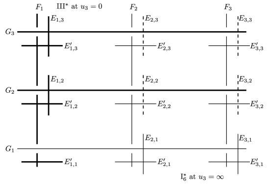
Figure 3. Fibration 3

5. Fibration 5

An elliptic parameter for Fibration 5 is given by

(5.1) $$u_{5}=y_{1}.$$

It is clear that this elliptic parameter defines a fibration having three singular fibers all of types $\operatorname{IV}^{*}$ at $u_{5}=1,-1$ and $\infty$ (the bold lines in Figure 4) from (2.7). Furthermore the fibration is induced by the composition of the first projection $C^{1}_{\omega}\times C^{2}_{\omega}\to C^{1}_{\omega}$ and the covering map of degree three $p_{1}:C^{1}_{\omega}\to\mathbb{P}^{1}$ in (3.7).

The following simple coordinate change

(5.2) $$X=(u_{5}^{2}-1)t,\quad Y=(u_{5}^{2}-1)^{2}y_{2}$$

converts the equation (2.6) into the Weierstrass equation for Fibration 5

(5.3) $$Y^{2}=X^{3}+(u_{5}^{2}-1)^{4}.$$

The curve $G_{1},\,G_{2}$ and $G_{3}$ correspond to the zero section, 3-torsion rational points $(0,(u_{5}^{2}-1)^{2})$ and $(0,-(u_{5}^{2}-1)^{2})$, respectively (the dotted lines in Figure 4).

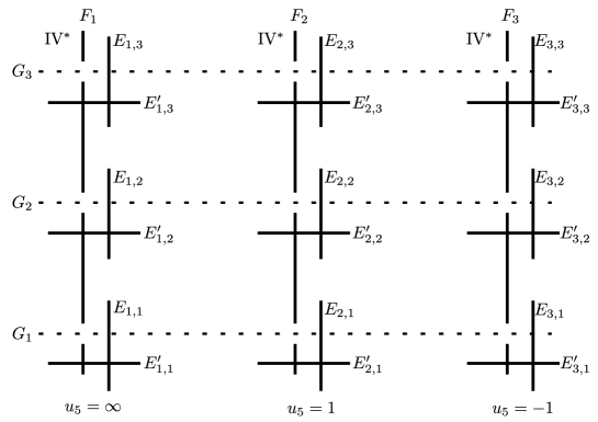
Figure 4. Fibration 5

6. Fibration 6

An elliptic parameter for Fibration 6 is given by

(6.1) $$u_{6}=t.$$

Since we gave the divisor of $t$ in (2.7), we know that the zero divisor $(u_{6})_{0}$ is the singular fiber of type $\operatorname{I}_{12}$ (the bold lines in Figure 5) and the polar divisor $(u_{6})_{\infty}$ is the singular fiber of $\operatorname{I}_{3}^{*}$ (the thin lines in Figure 5). The curves $E_{1,2},E_{1,3},E^{\prime}_{2,1}$ and $E^{\prime}_{3,1}$ (the dotted lines in Figure 5) are all the sections. Choosing $E_{1,2}$ as the zero section of the group structure, we obtain the Weierstrass equation for Fibration 6

(6.2) $$Y^{2}=X^{3}-2(u_{6}^{3}-2)X^{2}-u_{6}^{6}X,$$

where the change of variables is given by

(6.3) $$X=\frac{t^{3}(y_{2}+1)}{y_{2}-1},\quad Y=\frac{2t^{3}y_{1}(y_{2}+1)}{y_{2}-1}.$$

Besides the two singular fibers of type $\operatorname{I}_{12}$ at $u_{6}=0$ and of type $\operatorname{I}_{3}^{*}$ at $u_{6}=\infty$, there are three $\operatorname{I}_{1}$ fibers at $u_{6}=1,\omega$ and $\omega^{2}$. The Mordell-Weil group of the fibration is isomorphic to $\mathbb{Z}/4\mathbb{Z}$. The curve $E_{1,3}$ corresponds to the rational point $(0,0)$ of order two, and remaining curves $E^{\prime}_{2,1}$ and $E^{\prime}_{3,1}$ correspond to the rational points $(u_{6}^{3},2u_{6}^{3}),\,(u_{6}^{3},-2u_{6}^{3})$ of order four, respectively.

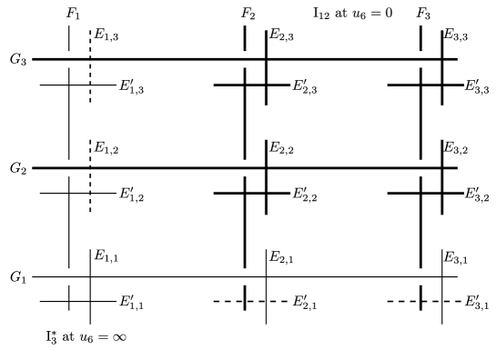
Figure 5. Fibration 6

7. Fibration 4

To obtain the Weierstrass equation for Fibration 4, we use a 2-neighbor step from Fibration 3. For more detail about 2-neighbor step, we refer to [5, 9, 11].

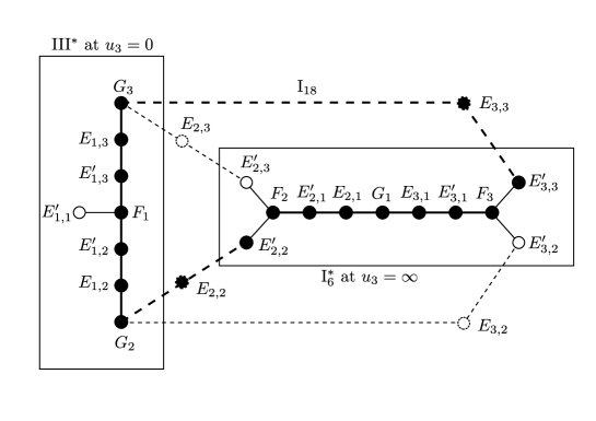
Figure 6. 2-neighbor from Fibration 3 to Fibration 4

We compute explicitly the elements of $\mathcal{O}_{X_{3}}(F)$ where

(7.1) $$F =E_{2,2}+G_{2}+E_{1,2}+E_{1,2}^{\prime}+F_{1}+E_{1,3}^{\prime}+E_{1,3}+G_{3}+E_{3,3}+E_{3,3}^{\prime}+F_{3}$$

$$\quad+E_{3,1}^{\prime}+E_{3,1}+G_{1}+E_{2,1}+E_{2,1}^{\prime}+F_{2}+E_{2,2}^{\prime}$$

is the class of the fiber of type $\operatorname{I}_{18}$ we are considering. The linear space $\mathcal{O}_{X_{3}}(F)$ is 2-dimensional, and the ratio of two linearly independent elements is an elliptic parameter for $X_{3}$. Since $1$ is an element of $\mathcal{O}_{X_{3}}$, we may find a non-constant element of $\mathcal{O}_{X_{3}}(F)$. Then it will be an elliptic parameter of Fibration 4. Let us $u_{4}^{\prime}\in\mathcal{O}_{X_{3}}(F)$ be a non-constant. The function $u_{4}^{\prime}$ has a simple pole along $E_{2,2}$ and $E_{3,3}$, which are the zero section and 2-torsion of Fibration 3. Also, it has a simple pole along $G_{2}$, the identity component of the fiber at $u_{3}=0$, a simple pole along $E_{3,3}^{\prime}$, the identity component of the fiber at $u_{3}=\infty$. Therefore we can put

(7.2) $$u_{4}^{\prime}=\frac{\frac{Y}{X}+A_{0}+A_{1}u_{3}+A_{2}u_{3}^{2}}{u_{3}},$$

where the variables $u_{3},X,Y$ are given by (4.1) and (4.5). Assume $A_{1}=0$, since $1$ is an element of $\mathcal{O}_{X_{3}}(F)$. To obtain the coefficients $A_{0}$ and $A_{2}$, we look at the order of vanishing along the non-identity components of fibers at $u_{3}=\infty$. The function $u_{4}^{\prime}$ does not have any pole along $E_{3,2}^{\prime}$, which intersects with the section $E_{3,2}$ of the fibration 3 at $u_{3}=\infty$. Hence $u_{4}^{\prime}$ has no pole at $(X,Y,u_{3})=(1,-1,\infty)$, and that gives us $A_{2}=0$. Similarly, the component $E_{2,3}^{\prime}$, which intersects with the section $E_{2,3}$, gives us $A_{0}=0$. Consequently, we have a new elliptic parameter

(7.3) $$u_{4}^{\prime}=\dfrac{Y}{u_{3}X},$$

where the variables $u_{3},X,Y$ are given by (4.1) and (4.5). Solving for $Y$ and substituting into the Weierstrass equation (4.4), after suitable coordinate changes we have the following

(7.4) $$y^{2}=x^{3}+\frac{1}{4}({u_{4}^{\prime}}^{2}x-16)^{2}.$$

Although this is a Weierstrass equation for Fibration 4, for latter calculations, we put

(7.5) $${u_{4}}^{\prime}=\frac{2}{u_{4}},\;x=\frac{2^{2}X}{u_{4}^{4}},\;y=\frac{2^{3}Y}{u_{4}^{6}}$$

and obtain another Weierstrass equation for Fibration 4

(7.6) $$Y^{2}=X^{3}+(X-u_{4}^{6})^{2}.$$

The change of variables is given by

(7.7) $$u_{4}=\dfrac{t}{y_{1}+y_{2}},\;X=\frac{(y_{1}^{2}-1)t^{3}}{(y_{1}+y_{2})^{4}},\;Y=\frac{(y_{1}^{2}y_{2}+2y_{1}+y_{2})t^{6}}{(y_{2}^{2}-1)(y_{1}+y_{2})^{6}}.$$

The fibration has singular fibers of type $\operatorname{I}_{18}$ at $u_{4}=0$ and of type $\operatorname{I}_{1}$ at the zeros of $27u_{4}^{6}+4=0$. The zero section corresponds to the divisor $E^{\prime}_{1,1}$. The 3-torsion rational points $(0,u_{4}^{6})$ and $(0,-u_{4}^{6})$ correspond to the divisors $E^{\prime}_{3,2}$ and $E^{\prime}_{2,3}$, respectively. The free rational points $(2u_{4}^{3},u_{4}^{4}+2u_{4}^{3})$ and $(-2u_{4}^{6},u_{4}^{3}-2u_{4}^{3})$ correspond to the divisors $E_{3,2}$ and $E_{2,3}$, respectively with the relation $E_{2,3}+E_{3,2}=E^{\prime}_{2,3}$ in the Mordell-Weil group. Since the height of $E_{2,3}$ is equal to $\frac{3}{2}$, $E_{2,3}$ generates the Mordell-Weil lattice of the fibration.

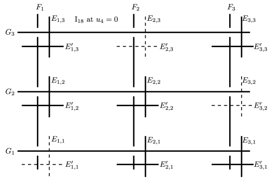
Figure 7. Fibration 4

8. Fibration 2

We obtain the following elliptic parameter $u_{2}^{\prime}$ for Fibration 2 by a 2-neighbor step from Fibration 4 (see Figure 8).

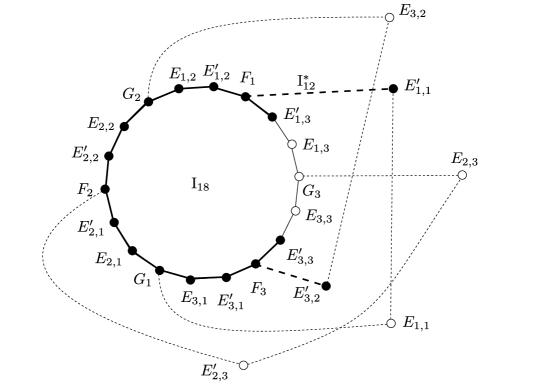
Figure 8. 2-neighbor form Fibration 4 to Fibration 2

(8.1) $$u_{2}^{\prime}=\frac{u_{4}^{6}+X+Y}{u_{4}^{2}X}$$

The variables $u_{4},X,Y$ are given by (7.7). Then we get the following Weierstrass equation for Fibration 2.

(8.2) $$y^{2}=x^{3}+2({u_{2}^{\prime}}^{3}-4)x^{2}+16x.$$

We put

(8.3) $$u_{2}^{\prime}=\frac{2}{u_{2}},\;x=\frac{2^{2}X}{u_{2}^{4}},\;y=\frac{2^{3}Y}{u_{2}^{6}}$$

and obtain another Weierstrass equation for Fibration 4.

(8.4) $$Y^{2}=X^{3}-2(u_{2}^{3}-2)X^{2}-u_{2}^{8}X.$$

The change of variables is given by

(8.5) $$u_{2}=\frac{2t^{2}}{(y_{2}+1)(y_{1}^{2}+2y_{1}+2y_{2}-1)},$$

$$X=-\frac{32(y_{1}-1)^{2}(y_{2}-1)^{3}t^{2}}{(y_{2}+1)^{2}(y_{1}^{2}+2y_{1}+2y_{2}-1)^{4}},$$

$$Y=-\frac{128(y_{1}-1)^{3}(y_{2}-1)^{4}(y_{1}+1)(y_{1}+y_{2})}{(y_{2}+1)^{2}(y_{1}^{2}+2y_{1}+2y_{2}-1)^{5}}.$$

The zero divisor $\left(u_{4}\right)_{0}$ is the singular fiber of type $\operatorname{I}_{12}^{*}$ (the bold lines in Figure 9). The polar divisor $\left(u_{4}\right)_{\infty}=G_{3}+E_{2,3}+Q_{2}$ is the singular fiber of type $\operatorname{I}_{3}$ (the thin lines in Figure 9), where the divisor $Q_{2}$ is the lifting of the curve $y_{1}^{2}+2y_{1}+2y_{2}-1=0$ on $\mathbb{P}^{1}\times\mathbb{P}^{1}$ by the map $\pi$ in §3. Besides these two singular fibers, there are three $\operatorname{I}_{1}$ fibers at $u_{2}=1,\omega$ and $\omega^{2}$. The zero section corresponds to the divisor $E_{1,3}$. The 2-torsion rational point $(0,0)$ corresponds to the divisor $E_{3,3}$.

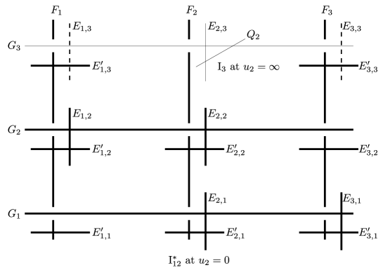
Figure 9. Fibration 2

Remark 2.

We give a Weierstrass equation for Fibration 6 in §6. Comparing the equations (8.4) and (6.2), we know easily that Fibration 2 is a quadratic twist of Fibration 6. This is the reason why we adopt the equation (8.4) as the Weierstrass equation for Fibration 2 rather than the equation (8.2).

Acknowledgements.

The computer algebra system Maple and Maple Library “Elliptic Surface Calculator” written by Professor Masato Kuwata [6] were used in the calculation for this paper. The author would like to thank the developers of these programs.

References

- [1] Sang Yook An, Seog Young Kim, David C. Marshall, Susan H. Marshall, William G. McCallum and Alexander R. Perlis, “Jacobians of genus one curves”, J. Number Theory 90 (2001), no. 2, 304-315.
- [2] A. P. Braun, Y. Kimura and T. Watari, “On the classification of elliptic fibrations modulo isomorphism on surfaces with large Picard number”, arXiv:1312.4421.
- [3] I. Connell, Addendum to a paper of K. Harada and M.-L. Lang, “Some elliptic curves arising from the Leech lattice” [J. Algebra 125 (1989), no. 2, 298–310], J. Algebra 145 (1992), 463-467.
- [4] K. Kodaira, “On compact analytic surfaces II”, Ann. of Math. 77, no.3 (1963), 545-560.
- [5] A. Kumar, “Elliptic fibrations on a generic Jacobian Kummer surface”, arXiv:1105.1715.
-
[6]
M. Kuwata, “Maple Library ’Elliptic Surface
Calculator’ ”,
http://c-faculty.chuo-u.ac.jp/~kuwata/ESC.php. - [7] M. Kuwata and T. Shioda, “Elliptic parameters and defining equations for elliptic fibrations on a Kummer surface”, Algebraic geometry in East Asia-Hanoi (2005), 177-215, Adv. Stud. Pure Math., 50, Math. Soc. Japan, Tokyo, 2008.
- [8] K. Nishiyama, “The Jacobian fibrations on some surfaces and their Mordell-Weil groups”, Japan. J. Math. (N.S.) 22 (1996), no. 2, 293-347.
- [9] T. Sengupta, “Elliptic fibrations on supersingular surface with Artin invariant in characteristic ”, arXiv:1204.6478.
- [10] T. Shioda and H. Inose and, On singular surfaces, Complex analysis and algebraic geometry, 119–136. Iwanami Shoten, Tokyo, 1977.
- [11] K. Utsumi, “Weierstrass equations for Jacobian fibrations on a certain surface”, Hiroshima Math. J. 42, (2012), no. 3, 355-383.