Improving offline evaluation of contextual bandit algorithms
via bootstrapping techniques

Abstract

In many recommendation applications such as news recommendation, the items that can be recommended come and go at a very fast pace. This is a challenge for recommender systems (RS) to face this setting. Online learning algorithms seem to be the most straight forward solution. The contextual bandit framework was introduced for that very purpose. In general the evaluation of a RS is a critical issue. Live evaluation is often avoided due to the potential loss of revenue, hence the need for offline evaluation methods. Two options are available. Model based methods are biased by nature and are thus difficult to trust when used alone. Data driven methods are therefore what we consider here. Evaluating online learning algorithms with past data is not simple but some methods exist in the literature. Nonetheless their accuracy is not satisfactory mainly due to their mechanism of data rejection that only allow the exploitation of a small fraction of the data. We precisely address this issue in this paper. After highlighting the limitations of the previous methods, we present a new method, based on bootstrapping techniques. This new method comes with two important improvements: it is much more accurate and it provides a measure of quality of its estimation. The latter is a highly desirable property in order to minimize the risks entailed by putting online a RS for the first time. We provide both theoretical and experimental proofs of its superiority compared to state-of-the-art methods, as well as an analysis of the convergence of the measure of quality.

1 Introduction

Under various forms, and under various names, recommendation has become a very common activity over the web. One can think of movie recommendation (Netflix), e-commerce (Amazon), online advertising (everywhere), news recommendation (Digg), personalized radio stations (Pandora) or even job recommendation (LinkedIn)… All these applications have their own characteristics. Yet the common key idea is to take advantage of some information we may have on a user (profile, demographics, time of the day etc.) in order to identify the most attractive content to serve him/her in a given context. Note that an element of content is generally referred to as an item. To perform recommendation, a piece of software called a recommender system (RS) can use past user/item interactions such as clicks or ratings. In particular, the typical approach to recommendation is to train a predictor of ratings and/or clicks of users on items on past data and use the resulting predictions to make personalized recommendations. This approach is based on the implicit assumption that past behavior can be used to predict future behavior.

In this paper we consider a recommendation applications in which the aforementioned assumption is not reasonable. We refer to this setting as dynamic recommendation. In dynamic recommendation, only a few tens of different items are available for recommendation at any given moment. These items have a limited lifetime and are continuously replaced by new ones, with different characteristics. We also consider that the tastes of users change, sometimes dramatically due to external parameters that we do not control. Many examples of dynamic recommendation exist on the web. The most popular one is news recommendation that can be found on specialized websites such as Digg or on general web portals (Yahoo!) and websites of various media (newspapers, TV channels…). Other examples can be mentioned such as private auctions in which the user can buy a limited set of items that changes everyday. Another example is a RS that can only recommend the K most recent items (this may apply to movies, videos, songs…). This problem has begun to be addressed recently with online learning solutions, by considering the contextual bandit framework. Nonetheless this is not the case in most of the recommendation literature. In all the textbooks, dynamic recommendation is handled with content-based recommendation. The idea is to consider an item as a set of features and to try to predict the taste of a user with regards to these features, using an offline predictor as before. Yet we argue that although this can be a good idea in some special cases, this is not the way to go in general:

1. It requires a continuous labeling effort of new items.

2. We are limited by what the expert labels: things can be hard to label such as the appeal for a picture, the quality of a textual summary, etc.

3. Tastes are not static: the appeal of a user to some kind of news can be greatly impacted by the political context. Similarly the appeal towards clothing can be impacted by fashion, movie stars etc.

For such systems, the best way to compare the performance of two algorithms is to perform A/B testing on a subset of the web audience (Kohavi et al., 2009). Yet there is almost no e-commerce website that would let a new RS go live just for testing, even on a small portion of the audience for fear of hurting the user experience and loosing money. The entailed engineering effort can also be discouraging. Therefore being able to evaluate offline a RS is crucial. In classical recommendation, the measures of prediction accuracy and other metrics that can be computed on past data are well accepted and trusted in the community. Nevertheless for the reasons we gave above, they are irrelevant for online learning algorithms designed for dynamic recommendation. This paper is about the offline evaluation of such algorithms. Some fairly simple replay methodologies do exist in the literature. Nonetheless they have a well known, yet very little studied drawback which is that they use a very small portion of the data at hand. One may argue that the tremendous amount of data available with web applications makes this a marginal problem. Yet in this paper we will exhibit that this is a major issue that generates a huge bias when evaluating online learning algorithms for dynamic recommendation. Furthermore we will explain that acquiring more data does not solve the problem. Then we will propose a solution to this issue, that builds on the previously introduced methods and on different elements of bootstrapping theory. This solution is backed by a theoretical analysis as well as an empirical study. They both clearly exhibit the improvement in terms of evaluation accuracy brought by our new method. Furthermore the use of bootstrapping allows us to estimate the distribution of our estimation and therefore to get a sense of its quality. This is a highly desirable property, especially considering that such an evaluation method is designed in order to decide whether we should risk putting a new algorithm online. The fast theoretical convergence of this estimation is also proved in our analysis. Note that the experiments are run on synthetic data, for reasons that we will detail and also on a large publicly available dataset.

2 Background on bandits and notations

We motivated the need for online learning solutions in order to deal with dynamic recommendation. A natural way to model this situation is as a reinforcement learning problem (Sutton & Barto, 1998), and more precisely using the contextual bandit framework (Lu et al., 2010) that was introduced for the very purpose of news recommendation.

2.1 Contextual Bandits

The bandit problem is also known in the literature as the multi-arm bandit problem and other variations. This problem can be traced back to Robbins and Munro in 1952 (Robbins, 1952) and even Thompson in 1933 (Thompson, 1933). There are many variations in the definition of the problem; the contextual bandit framework as it is defined in (Langford & Zhang, 2007) is as follows:

Let $\cal X$ be an arbitrary input space and ${\cal A}=\left\{1..K\right\}$ be a set of $K$ actions. Let ${\cal D}$ be a distribution over tuples $(x,\vec{r})$ with $x\in{\cal X}$ and $\vec{r}\in\left\{0,1\right\}^{K}$ a vector of rewards: in the $(x,\vec{r})$ pair, the $j^{\mbox{\scriptsize th}}$ component of $\vec{r}$ is the reward associated to action $a_{j}$, performed in the context $x$. In recommendation, the context is the information we have on the user (session, demographics, profile etc.) and an action is the recommendation of an item.

A contextual bandit game is an iterated game in which at each round $t$:

• $(x_{t},\vec{r_{t}})$ is drawn from ${\cal D}$.

• $x_{t}$ is provided to the player.

• The player chooses an action $a_{t}\in{\cal A}$ based on $x_{t}$ and on the knowledge it gathered from the previous rounds of the game.

• The reward $\vec{r_{t}}[a_{t}]$ is revealed to the player whose score is updated.

• The player updates his knowledge based on this new experience.

It is important to note the partial observability of this game: the reward is known only for the action performed by the player. This is what makes offline evaluation a complicated problem. A typical goal is to maximize the sum of reward obtained after $T$ steps. To succeed a player has to learn about ${\cal D}$ and try to exploit that information. Therefore at time $t$, a player faces a classical exploration/exploitation dilemma: either perform an action he is uncertain about in order to improve his model of ${\cal D}$ (explore), either perform the action he believe to be optimal, although it may not be (exploit).

A simpler variant of this problem in which no contextual information is given, called the multi armed bandit problem (MAB) was extensively studied in the literature. One can for instance mention the UCB algorithm (Auer et al., 2002) that optimistically deals with the dilemma by performing the action with higher upper confidence bound on the estimated reward expectation. The contextual bandit problem is less studied due to the additional complexity and additional assumptions entailed by the context space. The most popular algorithm is without doubt LinUCB (Li et al., 2010), although a few others exist such as epoch-greedy (Langford & Zhang, 2007). LinUCB is basically an extension of the classical UCB that uses the contexts under the assumption of normality and that ${\cal X}=\mathbb{R}^{d}$. The reward expectation of an action is estimated via a linear regression on the context vectors and the confidence bound is computed using the dispersion matrix of the context vectors. These two state-of-the-art algorithms are the ones we will evaluate when running experiments.

2.2 Evaluation

We define a contextual algorithm $A$ as taking as input an ordered list of $(x,a,r)$ triplets (history) and outputting a policy $\pi$. A policy $\pi$ maps $\cal{X}$ to ${\cal A}$, that is chooses an action given a context. Note that we are also interested in evaluating policies. In our setting which is the most popular one, an algorithm is said optimal when maximizing the expectation of the sum of rewards after $T$ steps:

$$G_{A}(T,{\cal D})\stackrel{{\scriptstyle\text{\tiny def}}}{{=}}\mathbb{E}_{\cal D}\sum_{t=1}^{T}\vec{r_{t}}[A(x_{t})].$$

For convenience, we define the per-trial payoff as the average click rate after $T$ steps:

$$g_{A}(T,{\cal D})\stackrel{{\scriptstyle\text{\tiny def}}}{{=}}\frac{G_{A}(T)}{T}$$

Note that for a static algorithm (ie. that always outputs the same policy $\pi$), we have that:

$$\forall T,g_{A}(T,{\cal D})=g_{A}(1,{\cal D})\stackrel{{\scriptstyle\text{\tiny def}}}{{=}}g_{A}({\cal D}).$$

Note that from this point on, we will simplify the notations by systematically dropping ${\cal D}$. $g_{A}(T)$ is thus the quantity we wish to estimate as the measure of performance of a bandit algorithm.

In order to minimize the risks entailed by playing live a new algorithm, we are also interested in the quality of the estimation. Bootstrapping will enable us to estimate it. To do so we need additional notations. $CTR_{A}(T)$ denotes the distribution of the per-trial payoff of $A$ after $T$ steps (so $g_{A}(T)$ is its mean). Besides estimating $g_{A}(T)$, our second goal is the computation of an estimator quality assessment $\xi\left(CTR_{A}(T)\right)$. Note that typically, $\xi$ can be a quantile, a standard error, a bias or what we will consider here for simplicity: a confidence region around the mean of $CTR_{A}(T)$ (aka $g_{A}$).

3 The time acceleration issue with replay methodologies

This section describes the replay methodology, that we call replay and that was introduced by (Langford et al., 2008) and analyzed for the setting we consider by (Li et al., 2011). This section also highlights the method’s limitations that we overcome in this paper and is crucial to understand the significance of our contribution.

First of all, as (Li et al., 2011), we assume that we have a dataset $S$ that was acquired online using an random uniform allocation of the actions for $T$ steps. This data collection phase can be referred as exploration policy and is our unique information on ${\cal D}$. This random decision making implies that any point in ${\cal X}\times{\cal A}$ has a non null probability to belong to $S$; this allows the evaluation of any policy. In a nutshell, the replay methodology on such a dataset works as follows: for each record $(x_{t},a_{t},r_{t})$ in $S$, the algorithm $A$ is asked to choose an action given $x_{t}$. If this action is $a_{t}$, $r_{t}$ is revealed to $A$ and taken into account to evaluate its performance. If the action is different, the record is discarded. This method is proved to be unbiased in some cases (Li et al., 2011). Note that the fact it needs the data to be acquired uniformly at random is quite restrictive. This problem is well studied and replay can be extended to allow the use of data acquired by a different but known logging policy at a cost of increased variance (Langford et al., 2008). Some work has been done to reduce this variance and even allow the use of data for which the logging policy is unknown (Dudík et al., 2011; Strehl et al., 2010). Note also that if the evaluated bandit algorithm is close from the logging policy, we may even further reduce the variance (Bottou et al., 2012). Finally there exist ways to adapt this method to the case where a list of items can be recommended (Langford et al., 2008). Although we do not take into account these considerations and keep the simplest assumption in this paper for clarity, our method is based on the same ideas as replay and could therefore be extended similarly as what is presented in the works we just cited.

Another issue with replay is well-known but not studied at all up to our knowledge. In average, only $\frac{T}{K}$ records are used. Therefore replay outputs an estimate $\hat{g_{A}}\left(\frac{T}{K}\right)$ which follows the distribution $CTR_{A}\left(\frac{T}{K}\right)$ of mean $g_{A}\left(\frac{T}{K}\right)$. It is important to have in mind that $g_{A}\left(\frac{T}{K}\right)=g_{A}\left(T\right)$ if and only if $T=+\infty$ or $A$ is a static policy. See figure 1 for a visual example of this problem. Note that in any situation except $K=1$, $CTR_{A}\left(\frac{T}{K}\right)\neq CTR_{A}\left(T\right)$, and the same thing goes for the confidence region $\xi$.

One may argue that when evaluating a RS, plenty of data is available and therefore that $T$ is almost infinite. Consequently one may also consider replay to be almost unbiased. This is true with the classical contextual bandit framework considered in the literature. With dynamic recommendation, the main application for this method, this could not be more wrong. Indeed, we argued that in this context, everything changes, especially the available items. For instance, in news recommendation a news remains active from a few hours to two days and its CTR systematically decreases over time (Agarwal et al., 2009). Moreover we also mentioned reasons to believe that the user tastes may change as well. Therefore when evaluating a contextual bandit algorithm, we want to evaluate its behavior against a very dynamic environment and in particular its ability to adapt to it. The use of replay in such a context is often justified by the fact that the environment can be considered static for small periods of time. This is not necessary but makes the understanding of our point easier. When an algorithm faces a ”static” region of a dataset of size $T_{i}$, when being replayed, it only has $\frac{T_{i}}{K}$ instead of $T_{i}$ steps to learn and exploit that knowledge. It is impossible to solve this problem by considering more data since new data would concern the next region, where different news with different CTR are available for recommendation, and potentially users with different tastes. In fact whatever assumptions we use to characterize how things evolve, using replay is equivalent to playing an algorithm with time going $K$ times faster than in reality. This generates a huge bias. Note that it is most likely because of time acceleration that a non-contextual algorithm which looks a lot like UCB won a challenge evaluated by replay on the Yahoo! R6B dataset (Yahoo! Research, 2012) (news recommendation). See chapter 4 of Nicol (Nicol, 2014) for more details.

As a conclusion, we consider in this work a classical contextual bandit framework with a fixed number of steps $T$. We assume that no more than $T$ records can be acquired. Yet it is clear that if we manage to deal with this problem without adding data, we would also be able to deal as well with the problem of evaluating dynamic recommendation for which using more data may not be possible.

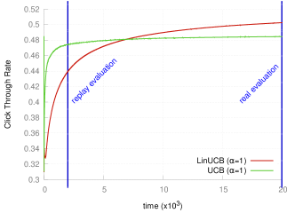
Figure 1: CTR over time of LinUCB (good model, slow learning) and UCB (too simple model but fast learning) when played $T=20,000$ times on $\cal D$ (see section 6.1 for the model). Replay emulates only $\frac{T}{K}$ steps (see blue line) which is clearly misleading if we are interested in performance over $T$ steps.

4 Bootstrapped Replay on Expanded Data

Now that the shortcoming of the replay method has been understood, we look for an other offline evaluation protocol that does not suffer from the time acceleration issue. The idea we propose stems from the idea of bootstrapping, introduced by (Efron, 1979). Thus let us remind the standard bootstrap approach. Basically, the idea is to compute the empirical distribution $\hat{{\cal D}}_{T}$ of an estimator $\hat{\theta}_{T}$ computed on $T$ observations. To do so, one only has access to a dataset $S$ of size $T$. Therefore $B$ new datasets $S_{1},...S_{B}$ of size $T$ are generated by making bootstrap resamples from $S$. A bootstrap resample is generated via drawing $T$ samples with replacement. Note that this bootstrap procedure is a way to approximate ${\cal D}$, the underlying distribution of the data. Computing $\hat{\theta}_{T}$ on all the $S_{i}$ yields $\widehat{CTR}(T)$, an estimation of $CTR(T)$. From a theoretical point of view and under mild assumptions, $\xi\left(\widehat{CTR}(T)\right)$ converges with no bias at a speed in $O(1/T)$. This means that under a assumption of the concentration speed of a statistic we are able to estimate the confidence interval of the mean of the statistic much faster than its mean. Recall that $\xi$ can be any measure of accuracy (defined in terms of bias, variance, confidence intervals, …) over the statistic we want to study. Here we are interested in confidence intervals over $CTR_{A}(T)$.

Algorithm 1 Bootstrapped Replay on Expanded Data (BRED).
We sketch this algorithm so that it looks very much like replay in (Li et al., 2011). Thus an algorithm is a function that maps an history of events $h^{(b)}$ to a policy $\pi$ which itself maps contexts to actions. This makes the learning process of the algorithm appear clearly. A computationally efficient implementation would be slightly different. Notice also that for clarity, we only compute $\hat{g}_{A}(T)$ and omit ${\widehat{CTR}}_{A}(T)$.

Input

• A (contextual) bandit algorithm $A$

• A dataset $S$ of $T$ triplets $(x,a,r)$

• An integer $B$

Output: An estimate of $g_{A}$

  $h^{(b)}\leftarrow\emptyset$, $\forall b\in\left\{1..B\right\}$ /*empty history*/

  $\widehat{G}_{A}^{(b)}\leftarrow 0$, $\forall b\in\left\{1..B\right\}$

  $T^{(b)}\leftarrow 0$, $\forall b\in\left\{1..B\right\}$

  /* Bootstrap loop*/

  for $b\in\left\{1..B\right\}$ do

     /* estimation of $CTR_{A}^{(b)}(T)$*/

     for $i\in\left\{1..T\times{}K\right\}$  do

        Sample with replacement $(x,a,r)$ of $S$

        $x\leftarrow$ JITTER$(x)$ /*optional*/

        $\pi\leftarrow A(h^{(b)})$

        if $\pi(x)=a$ then

           add $(x,a,r)$ to $h^{(b)}$

           $\widehat{G}_{A}^{(b)}\leftarrow\widehat{G}_{A}^{(b)}+r$

           $T^{(b)}\leftarrow T^{(b)}+1$

        end if

     end for

  end for

  return $\frac{1}{B}\sum\limits_{b=1}^{B}\frac{\widehat{G}_{A}^{(b)}}{T^{(b)}}$

The core idea of the evaluation protocol we propose in this paper is inspired by bootstrapping and inherits its theoretical properties. Using our notations, here is the description of this new method. From a dataset of size $T$ with $K$ possible choices of action at each step - we do not require $K$ to be constant over time -,we generate $B$ datasets of size $K.T$ by sampling with replacement, following the non-parametric bootstrap procedure. Then for each dataset $S_{b}$ we use the classical replay method to compute an estimate $\hat{g_{A}}^{(b)}(T)$. Therefore $A$ is evaluated on $T$ records on average. This step can be seen as a subsampling step that allows to return in the classical bootstrap setting. Thus note that it would not work for a purely deterministic policy, that for obvious reason would not take advantage of the data expansion (an assumption in the formal analysis will reflect this fact). $\hat{g}_{A}(T)$ is given by averaging the $\hat{g_{A}}^{(b)}(T)$. Together, the $\hat{g_{A}}^{(b)}(T)$ are also an estimation of $CTR_{A}(T)$, the distribution of the CTR of $A$ after $T$ interactions with ${\cal D}$ on which we can compute our estimator quality assessment $\xi$. More formally, the bootstrap estimator of the density of $CTR_{A}(T)$ is estimated as follows:

$${\widehat{CTR}_{A}(T)}(x)=\frac{1}{B}\sum_{b=1}^{B}I\left(\sqrt{T}\left[\frac{\hat{g}_{A}^{(b)}(T)-\hat{g}_{A}(T)}{\hat{\sigma}_{A}(T)}\right]\leq x\right)$$

where $\hat{\sigma}_{A}(T)$ is the empirical standard deviation obtained when computing the bootstrap estimates $\hat{g_{A}}^{(b)}(T)$. The complete procedure, called Bootstrapped Replay on Expanded Data (BRED), is implemented in algorithm 1.

To complete the BRED procedure, one last detail is necessary. Each record of the original dataset $S$ is contained $K$ times in expectation in each expanded dataset $S_{b}$. Therefore a learning algorithm may tend to overfit which would bias the estimator. To prevent this from happening, we introduce a small amount of Gaussian noise on the contexts. This technique is known as jittering and is well studied in the neural network field (Koistinen & Holmström, 1992). The goal is the same, that is avoiding overfitting. In practice however it is slightly different as neural network are generally not learning online but on batches of data, each data being used several times during learning. In bootstrapping theory this technique is known as the smoothed bootstrap and was introduced by (Silverman & Young, 1987). We mentioned that the bootstrap resampling is a way to approximate ${\cal D}$. The smoothed bootstrap goes further by performing a kernel density estimation (KDE) of the data and sampling from it. Sampling from a KDE of the data where the kernel is Gaussian of bandwidth $h$ is equivalent to sampling a record uniformly from $S$ and applying a random noise sampled from ${\cal N}(0,h^{2})$, which is what jittering does. The usual purpose of doing so in statistics is to get a less noisy empirical distribution for the estimator. Note that here we perform a partially smoothed bootstrap as we only apply a KDE on the part of ${\cal D}$ that generates the contexts.

5 Theoretical analysis

In this section, we make a theoretical analysis of our evaluation method BRED. The core loop in BRED is a bootstrap loop; henceforth, to complete this analysis, we first restate the theorem 1 which is a standard result of the bootstrap asymptotic analysis (Kleiner et al., 2012). Notice a small detail: each bootstrap step estimates a realization of $CTR_{A}(T)$. The number of evaluations - which is also the number of non rejects - is a random variable denoted $T^{(b)}$.

Theorem 1.

Suppose that:

• $A$ is a recommendation algorithm which generates a fixed policy over time (this hypothesis can be weakened as discussed in remark 2),

• $K$ items may be recommended at each time step,

• $\xi\left(CTR_{A}(T)\right)$ admits an expansion as an asymptotic series

  $$\xi\left(CTR_{A}(T)\right)=z+\frac{p_{1}}{\sqrt{T}}+\ldots+\frac{p_{\alpha}}{T^{\alpha/2}}+o\left(\frac{1}{T^{\alpha/2}}\right)$$

  where $z$ is a constant independent of the distribution ${\cal D}$ (as defined in Sec. 2.1), and the $p_{i}$ are polynomials in the moments of $CTR_{A}(T)$ under ${\cal D}$ (this hypothesis is discussed and explained in remark 1),

• The empirical estimator $\xi\left({\widehat{C}TR}_{A}(T)\right)$ admits a similar expansion:

  $$\begin{split}z+\frac{\widehat{p}_{1}}{\sqrt{T}}+\ldots+\frac{\widehat{p}_{\alpha}}{T^{\alpha/2}}+O\left(\frac{1}{T^{\alpha/2}}\right).\end{split}$$ (1)

Then, for $T\leq T^{(b)}\times{}K$ and assuming finite first and second moments of $\widehat{CTR}_{A}(T)$, with high probability:

$$\begin{split}\left|\xi\left(CTR_{A}(T)\right)-\xi\left({\widehat{C}TR}_{A}(T)\right)\right|=\\ O\left(\frac{\mbox{Var}(\widehat{p}_{\alpha}^{(1)}-p_{\alpha}|D_{T})}{\sqrt{T\cdot B}}\right)+O\left(\frac{1}{T}\right)+O\left(\frac{1}{T\sqrt{T}}\right)\end{split}$$ (2)

where ${\cal D}_{T}$ is the resampled distribution of ${\cal D}$ using $T$ realizations.

Proof.

it is actually a straightforward adaptation of the proof of theorem 3 of (Kleiner et al., 2012). Also note that this theorem is a reformulation of the bootstrap main convergence result as introduced by (Efron, 1979). ∎

Now, we use theorem 1 to bound the error made by BRED in the theorem 2.

Theorem 2.

Assuming that

$$\xi\left(CTR_{A}(T)\right)=z+\frac{p_{1}}{\sqrt{T}}+\ldots+\frac{p_{\alpha}}{T^{\alpha/2}}+o\left(\frac{1}{T^{\alpha/2}}\right)$$

Then for algorithm $A$ producing a fixed policy over time, BRED applied on a dataset of size $T$ evaluates the expectation of the $CTR_{A}$ with no bias and with high probability for $B$ and $T$ large enough:

$$\left|\xi\left(CTR_{A}(T)\right)-\xi\left({\widehat{C}TR}_{A}(T)\right)\right|=O\left(\frac{1}{T}\right)$$

This means that the convergence of the estimator of $\xi\left(CTR_{A}(T)\right)$ is much faster than the convergence of the estimator of $g_{A}(T)$ (which is in $O(1/\sqrt{T})$. This will allow a nice control of the risk that $\hat{g}_{A}(T)$ may be badly evaluated.

The sketch of the proof of theorem 2 is the following: first we prove that the replay strategy is able to estimate the moments of the distribution of $CTR_{A}$ fast enough with respect to $T$. The second step consists in using classical results from bootstrap theory to guarantee the unbiased convergence of the aggregation $\widehat{CTR}_{A}(T)$ to the true distribution with an $O(\frac{1}{T})$ speed. The rational behind this is that the gap introduced by the subsampling will be of the order of $O(\frac{1}{\sqrt{TB}})$.

Proof.

At each iteration of the bootstrap loop (indexed by $b$), BRED is estimating the CTR using the replay method on a dataset of size $T^{\prime}=K\times{}T$. As the actions in $S$ were chosen uniformly at random, we have $\mathbb{E}(T^{(b)})=T^{\prime}/K=T$.

As the policy is fixed, we can use the multiplicative Chernoff’s bound as in (Li et al., 2011) to obtain for all bootstrap step $b$:

$$\mathbb{P}r{}\left(\left|T^{(b)}-T\right|\geq{\gamma_{1}T}\right)\leq\exp\left(-\frac{T\gamma_{1}^{2}}{3}\right)$$

for any $\gamma_{1}>0$ (where $\mathbb{P}r(e)$ denotes the probability of event $e$). A similar inequality can be obtained with $\mathbb{E}(\widehat{G}_{A})=Tg_{A}$:

$$\mathbb{P}r{}\left(\left|\widehat{G}_{A}-{Tg_{A}}\right|\geq{\gamma_{2}Tg_{A}}\right)\leq\exp\left(-\frac{Tg_{A}\gamma_{2}^{2}}{3}\right)$$

Thus with $\gamma_{1}=\sqrt{\frac{3}{T}\ln\frac{4}{\delta}}$ and $\gamma_{2}=\sqrt{\frac{3}{Tg_{A}}\ln\frac{4}{\delta}}$ using a union bound over probabilities, we have with probability at least $1-\delta$:

$${1-\gamma_{1}}\leq\frac{T^{(b)}}{T}\leq{1+\gamma_{1}}$$

$$g_{A}{1-\gamma_{2}}\leq\frac{\widehat{G}_{A}}{T}\leq g_{A}{1+\gamma_{2}}$$

which implies

$$\left|\frac{\widehat{G}_{A}}{T^{(b)}}-g_{A}\right|\leq\frac{(\gamma_{1}+\gamma_{2})g_{A}}{1-\gamma_{1}}=O\left(\sqrt{\frac{g_{a}}{T}}\ln\frac{1}{\delta}\right)$$

So with high probability the first moment of $\widehat{CTR}_{A}(T^{(b)})$ as estimated by the replay method admits an asymptotic expansion in $1/\sqrt{\mathbb{E}(T^{(b)})}=1/T$.

Now we need to focus on higher order terms. All the moments are finite because the reward distribution over ${\cal S}$ is bounded. Recall that by hypothesis $\xi\left(CTR_{A}(T)\right)$ admits a $\alpha^{{th}}$ order term:

$$p_{\alpha}=\mathbb{E}_{D}\left(CTR_{A}(T^{(b)})^{\alpha}\right)$$

The Chernoff’s bound can be applied to $|(T^{(b)})^{\alpha}-T^{\alpha}|$ and $|\widehat{G}_{A}^{\alpha}-T^{\alpha}g_{A}^{\alpha}|$ leading to

$$\left|\frac{\widehat{G}_{A}^{\alpha}}{(T^{(b)})^{\alpha}}-g_{A}^{\alpha}\right|=O\left({\left(\frac{g_{a}}{T}\right)}^{\frac{\alpha}{2}}\ln\frac{1}{\delta}\right)$$

With probability at least $1-\delta$. So for a large enough $T^{(b)}$, $\xi\left(\widehat{CTR}_{A}(T^{(b)})\right)$ admits a expansion in polynomials of $1/{\sqrt{T}}$. Thus theorem 1 applies and the aggregation of all the $\hat{g}^{(b)}_{A}(T^{(b)})$ allows an estimation of $CTR_{A}(T)$. For a large enough number of bootstrap iterations (the value of $B$ in BRED), we obtain a convergence speed in $O(1/T)$ with high probability, which concludes the proof. ∎

After this analysis, we make two remarks about the assumptions that were needed to establish the theorems.

Remark 1: The key point of the theorems is the existence of an asymptotic expansion of $CTR_{A}(T)$ and ${\widehat{CTR}}_{A}(T)$ in polynomials of $1/\sqrt{T}$. This is a natural hypothesis for $CTR_{A}(T)$ because the CTR is an average of bounded variables (probabilities of click). Note that the proof of theorem 2 shows that although $T^{(b)}$ is random the expansion remains valid anyway. For a contextual bandit algorithm $A$ producing a fixed policy, the mean is going to concentrate according to the central limit theorem (CLT). Furthermore this hypothesis, omnipresent in bootstrap theory (Efron, 1979), is for instance justified in econometrics by the fact that all the common estimators respect it (Horowitz, 2001). Yet this assumption is not verified for a static deterministic policy.

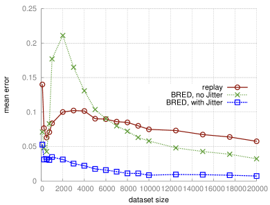
Figure 2: Mean absolute error of the CTR of LinUCB estimated by different methodologies. Conducted on artificial datasets as described by section 6.1. The lower, the better. Jittering ($h=\frac{50}{\sqrt{T}}$ here) is actually efficient to avoid overfitting issues. The rather small error rates for very small datasets are due to the fact that on too small datasets all the recommender algorithm tend to make random choices which are not very hard to evaluate.

Remark 2 Let us consider algorithms that produce a policy which changes over time (a learning algorithm in particular). After a sufficient amount of recommendations, a reasonable enough algorithm will produce a policy that will not change any longer (if the world is stationary). Thus again, the CLT will apply and we will observe a convergence of $\hat{g}_{A}(T)$ to its limit in $1/\sqrt{T}$. Nevertheless nothing holds true here when the algorithm is actually learning. This is due to the fact that the Chernoff bound no longer applies as the steps are not independent. However the behavior of classical learning algorithms are smooth, especially when randomized (see (Auer et al., 2003) for an example of a randomized version of UCB). (Li et al., 2011) argue that in this case convergence bounds may be derived for replay (which then could be applied to BRED) at the cost of a much more complicated analysis including smoothness assumptions. For non reasonable algorithms and thus in the general case, no guarantees can be provided. By the way note that a very intuitive way to justify Jittering is to consider that it helps the Chernoff bound being ”more true” in the case of a learning algorithm.

6 Experiments in realistic settings

As we proved that BRED has promising theoretical guarantees in the setting introduced in (Li et al., 2011), let us now compare its empirical performance to that of the replay method

6.1 Synthetic data and discussing Jittering

The first set of experiments was run on synthetic data. Indeed, we needed to be able to compare the errors of estimation of the two methods on various fixed size datasets relatively to the ground truth: an evaluation against the model itself. Before going any further, let us describe the model we used. It is a linear model with Gaussian noise (as in (Li et al., 2010)) and was built as follows:

• a fixed action set (or news set) of size $K=10$.

• The context space is $\mathcal{X}=\mathbb{R}^{15}$. Each context $x$ is generated as a sum $c+n$ where $c\sim\mathcal{N}(0,1)$ and $n\sim\mathcal{N}(0,\frac{1}{2})$.

• The CTR of a news $i$ displayed in a context $x$ is given linearly by $q_{i}+w_{i}^{T}c$. Note the non-contextual element $q_{i}$ and that the noise $n$ is ignored.

• Finally there are two kinds of news: (i) 4 “universal” news that are interesting in general like Obama is re-elected and for which $q_{i}\sim\mathcal{U}(0.4,0.5)$ is high and $w_{i}=0_{15}$. (ii) 6 specific news like New Linux distribution released for which $q_{i}\sim\mathcal{U}(0.1,0.2)$ is low and $w_{i}$ consists of zeros except for a number $m$ of relevant weights sampled from $\mathcal{N}(0,\frac{1}{5})$.

A non contextual approach would perform decently by quickly learning the $q_{i}$ values. Yet LinUCB (Li et al., 2010), a contextual bandit algorithm will do better by learning when to recommend the specific news. Figure 2 displays the results and interpretation of an experiment which consists in evaluating LinUCB($\alpha=1$) using the different methods. It is clear that BRED converges much faster than the replay method.

Remark: As it can be seen on Figure 2, jittering is very important to obtain good performance when evaluating a learning algorithm. Empirically, a good choice for the level of jitter seems to be a function in $O\left(\frac{1}{\sqrt{T}}\right)$, with $T$ the size of the dataset. Note that this is proportional to the standard distribution of the posterior of the data. The results confirm our intuition: jittering is very important when the dataset is small but gets less and less necessary as the dataset grows.

6.2 Real data

Adapting replay to a real life dataset, corresponding to dynamic recommendation is straightforward although it leads to biased estimations. BRED really needs the assumption of a static world in order to perform the bootstrap resamples. Therefore BRED needs to be run on successive windows of the dataset on which a static assumption can be made. This creates a bias/variance trade-off: if the windows are too big, some dynamic properties of the world may be erased (bias). On the contrary, too smalls window will lead to very variate bootstrap estimates. To simplify things, we ran experiments assuming a static world on small portions of the Yahoo! R6B dataset. We actually took the smallest number of portions such that a given portion has a fixed pool of news ($\approx 630$ portions). This experiment is similar to what is done in (Li et al., 2011): the authors measured the error of the estimated CTR of UCB ($\alpha=1$) by the replay method on datasets of various sizes relatively to what they call the ground truth: an evaluation of the same algorithm on a real fraction of the audience. As we obviously cannot do that, we used a simple trick. For each portion $i$ of size $T_{i}$ with $K_{i}$ news, we computed an estimation of the ground truth $g_{A}\left(\frac{T_{i}}{K_{i}}\right)$ by averaging the estimated CTR of UCB using the replay method on 100 random permutations of the data. For each portion the experiment consists in subsampling $T_{i}/K_{i}$ records and evaluating UCB using replay and BRED on this smaller dataset to estimate the ground truth using less data, faking time acceleration. The results and interpretation are shown on Figure 3: the better accuracy of BRED is very clearly illustrated.

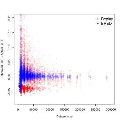
Figure 3: The difference between the estimated CTR and the actual one on some batches extracted from the Yahoo! R6B dataset for a UCB. Batches are build as explained in section 6.2. The closer to 0, the better. Please note that the replay method tends to under-estimate the true CTR for small batches. This is due to the fact that UCB does not have enough time to reach its actual CTR.

7 Conclusion

In this paper, we studied the problem of recommendation system evaluation, sticking to a realistic setting: we focused on obtaining a methodology for practical offline evaluation, providing a good estimate using a reasonable amount of data. Previous methods are proved to be asymptotically unbiased with a low speed of convergence on a static dataset, but yield counter-intuitive estimates of performance on real datasets. Here, we introduce BRED, a method with a much faster speed of convergence on static datasets (at the cost of loosing unbiasedness) which allows it to be much more accurate on dynamic data. Experiments demonstrated our point; they were performed on a publicly available dataset made from Yahoo! server logs and on synthetic data presenting the time acceleration issue. This paper was also meant to highlight the time acceleration issue and the misleading results given by a careless evaluation of an algorithm. Finally our method comes with a very desirable property in a context of minimizing the risks entailed by putting online a new RS: an extremely accurate estimation of the variability of the estimator it provides.

An interesting line of future work is the automatic selection of the Jittering bandwidth. Note that this problem is extensively studied in the context of KDE (Scott, 1992).

A possible extension of this work is to use BRED to build a ”safe controller”. Indeed, when a company uses a recommendation system that behaves according to a certain policy $\pi$ that reaches a certain level of performance, the hope is that when changing the recommendation algorithm, the performance will not drop. As an extension of the work presented here, it is possible to collect some data using the current policy $\pi$, compute small variations of $\pi$ with tight confidence intervals over their CTR and then replace the current policy $\pi$ with the improved one. This may be seen as a kind of “gradient” ascent of the CTR in the space of policies.

Supplementary material

The detailed implementation of replay using our notations is given in algorithm 2. Note that apart from notations, no modification are made with regards to the original presentation in (Langford et al., 2008; Li et al., 2011). Figure 4 is the same experiment as in section 6.1 but with a non-contextual algorithm UCB: this plot exhibits both the importance of Jittering and the improvement brought by our method compared to the state of the art.

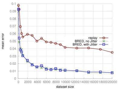
Figure 4: Mean of the absolute value of the difference between the true CTR of a UCB and the estimated one for different methodologies. Conducted on artificial dataset as described in the section 6.1 of the main paper. The lower, the better. Jittering is useless here because UCB does not use the context.

Algorithm 2 Replay method (Langford et al., 2008; Li et al., 2011).
Remark: for the sake of the precision of the specification of the algorithm, we use a history $h$ which is the list of triplets $(x,a,r)$ that have yet been used to estimate the performance of the algorithm $A$. The goal is to avoid hiding internal information maintenance in $A$; a real implementation may be significantly different for the sake of efficiency, by learning incrementally.

Input:

• A contextual bandit algorithm $A$

• A set $S$ of $L$ triplets $(x,a,r)$

Output: An estimate of $g_{A}$

  $h\leftarrow\emptyset$

  $\widehat{G}_{A}\leftarrow 0$

  $T\leftarrow 0$

  for $t\in\left\{1..L\right\}$ do

     Get the $t$-th element $(x,a,r)$ of $S$

     $\pi\leftarrow A(h)$

     if $\pi(x)=a$ then

        add $(x,a,r)$ to $h$

        $\widehat{G}_{A}\leftarrow\widehat{G}_{A}+r$

        $T\leftarrow T+1$

     end if

  end for

  return $\frac{\widehat{G}_{A}}{T}$

References

- Agarwal et al. (2009) Agarwal, Deepak, Chen, Bee-Chung, and Elango, Pradheep. Spatio-temporal models for estimating click-through rate. In Proceedings of the 18th international conference on World wide web(WWW), pp. 21–30, New York, NY, USA, 2009. ACM. ISBN 978-1-60558-487-4. doi: 10.1145/1526709.1526713.
- Auer et al. (2002) Auer, Peter, Cesa-Bianchi, Nicolò, and Fischer, Paul. Finite-time analysis of the multiarmed bandit problem. Machine Learning, 47:235–256, May 2002. ISSN 0885-6125.
- Auer et al. (2003) Auer, Peter, Cesa-Bianchi, Nicolò, Freund, Yoav, and Schapire, Robert E. The nonstochastic multiarmed bandit problem. SIAM J. Comput., 32(1):48–77, January 2003. ISSN 0097-5397. doi: 10.1137/S0097539701398375.
- Bottou et al. (2012) Bottou, Léon, Peters, Jonas, Quiñonero Candela, Joaquin, Charles, Denis X., Chickering, D. Max, Portugualy, Elon, Ray, Dipankar, Simard, Patrice, and Snelson, Ed. Counterfactual reasoning and learning systems. Technical report, arXiv:1209.2355, September 2012.
- Dudík et al. (2011) Dudík, Miroslav, Langford, John, and Li, Lihong. Doubly robust policy evaluation and learning. CoRR, abs/1103.4601, 2011.
- Efron (1979) Efron, B. Bootstrap methods: Another look at the jackknife. The Annals of Statistics, 7(1):1–26, 1979. ISSN 00905364. doi: 10.2307/2958830.
- Horowitz (2001) Horowitz, Joel L. The bootstrap. Handbook of econometrics, 5:3159–3228, 2001.
- Kleiner et al. (2012) Kleiner, Ariel, Talwalkar, Ameet, Sarkar, Purnamrita, and Jordan, Michael. The big data bootstrap. In Langford, John and Pineau, Joelle (eds.), Proceedings of the 29th International Conference on Machine Learning (ICML-12), ICML ’12, pp. 1759–1766, New York, NY, USA, July 2012. Omnipress. ISBN 978-1-4503-1285-1.
- Kohavi et al. (2009) Kohavi, Ron, Longbotham, Roger, Sommerfield, Dan, and Henne, Randal M. Controlled experiments on the web: Survey and practical guide. Journal of Data Mining and Knowledge Discovery, 18:140–181, 2009.
- Koistinen & Holmström (1992) Koistinen, Petri and Holmström, Lasse. Kernel regression and backpropagation training with noise. In Moody, John E., Hanson, Steve J., and Lippmann, Richard P. (eds.), Advances in Neural Information Processing Systems 4, pp. 1033–1039. San Francisco, CA: Morgan Kaufmann, 1992.
- Langford & Zhang (2007) Langford, John and Zhang, Tong. The epoch-greedy algorithm for multi-armed bandits with side information. In Proc. NIPS, 2007.
- Langford et al. (2008) Langford, John, Strehl, Alexander, and Wortman, Jennifer. Exploration scavenging. In Proceedings of the International Conference on Machine Learning (ICML), pp. 528–535, 2008.
- Li et al. (2010) Li, Lihong, Chu, Wei, Langford, John, and Schapire, Robert E. A contextual-bandit approach to personalized news article recommendation. In Proceedings of the 19th international conference on World wide web (WWW), pp. 661–670, New York, NY, USA, 2010. ACM. ISBN 978-1-60558-799-8. doi: 10.1145/1772690.1772758.
- Li et al. (2011) Li, Lihong, Chu, Wei, Langford, John, and Wang, Xuanhui. Unbiased offline evaluation of contextual-bandit-based news article recommendation algorithms. In King, Irwin, Nejdl, Wolfgang, and Li, Hang (eds.), Proc. Web Search and Data Mining (WSDM), pp. 297–306. ACM, 2011. ISBN 978-1-4503-0493-1.
- Lu et al. (2010) Lu, T., Pál, D., and Pál, M. Contextual multi-armed bandits. In Proc. of the 13 Artificial Intelligence and Statistics (AI & Stats), JMLR: W&CP 9, May 13-15 2010.
- Nicol (2014) Nicol, Olivier. Data-driven evaluation of Contextual Bandit algorithms and applications to Dynamic Recommendation. PhD thesis, Université Lille 1, Cité Scientifique, Villeneuve d’Ascq, France, 2014.
- Robbins (1952) Robbins, Herbert. Some aspects of the sequential design of experiments. Bulletin of the American Mathematical Society, 58(5):527–535, 1952.
- Scott (1992) Scott, D.W. Multivariate Density Estimation: Theory, Practice, and Visualization. Wiley Series in Probability and Statistics. Wiley, 1992. ISBN 9780471547709.
- Silverman & Young (1987) Silverman, BW and Young, GA. The bootstrap: To smooth or not to smooth? Biometrika, 74(3):469–479, 1987.
- Strehl et al. (2010) Strehl, Alexander L., Langford, John, Li, Lihong, and Kakade, Sham. Learning from logged implicit exploration data. In Proc. NIPS, pp. 2217–2225, 2010.
- Sutton & Barto (1998) Sutton, R.S. and Barto, A.G. Reinforcement Learning: An Introduction. Adaptive Computation and Machine Learning Series. MIT Press, 1998. ISBN 9780262193986.
- Thompson (1933) Thompson, W.R. On the likelihood that one unknown probability exceeds another in view of the evidence of two samples. Biometrika, 25(3–4):285––294, 1933.
- Yahoo! Research (2012) Yahoo! Research. R6B - Yahoo! front page today module user click log dataset, publicly released via the Yahoo! webscope program, 2012.