Running coupling effects in the evolution of jet quenching

Abstract

We study the consequences of including the running of the QCD coupling in the equation describing the evolution of the jet quenching parameter $\hat{q}$ in the double logarithmic approximation. To start with, we revisit the case of a fixed coupling, for which we obtain exact solutions valid for generic values of the transverse momentum (above the medium saturation scale) and corresponding to various initial conditions. In the case of a running coupling, we construct approximate solutions in the form of truncated series obtained via successive iterations, whose convergence is well under control. We thus deduce the dominant asymptotic behavior of the renormalized $\hat{q}$ in the limit of a large ‘evolution time’ $Y\equiv\ln(L/\lambda)$, with $L$ the size of the medium and $\lambda$ the typical wavelength of a medium constituent. We show that the asymptotic expansion is universal with respect to the choice of the initial condition at $Y=0$ and, moreover, it is remarkably similar to the corresponding expansion for the saturation momentum of a ‘shockwave’ (a large nucleus). As expected, the running of the coupling significantly slows down the increase of $\hat{q}$ with $Y$ in the asymptotic regime at $Y\gg 1$. For the phenomenologically interesting value $Y\simeq 3$, we find an enhancement factor close to 3, independently of the initial condition and for both fixed and running coupling.

I Introduction

The concept of ‘jet quenching’ encompasses a variety of phenomena, among which transverse momentum broadening, radiative energy loss, color decoherence, or medium–induced jet fragmentation, which accompany the propagation of a ‘hard probe’ (an energetic parton, or the jet generated by its evolution) through the dense QCD medium created at the intermediate stages of an ultrarelativistic nucleus–nucleus collision. The theoretical description of these phenomena within perturbative QCD reveals a remarkable universality Baier:1996kr ; Baier:1996sk ; Zakharov:1996fv ; Zakharov:1997uu ; Baier:1998kq ; Wiedemann:2000za ; Wiedemann:2000tf ; Arnold:2001ms ; Arnold:2002ja ; MehtarTani:2010ma ; MehtarTani:2011tz ; CasalderreySolana:2011rz ; Blaizot:2012fh ; Blaizot:2013hx ; Blaizot:2013vha : to leading order in $\alpha_{s}=g^{2}/4\pi$ (the QCD coupling, assumed to be small), they all depend upon the medium properties via a single quantity, known as the ‘jet quenching parameter’ $\hat{q}$. This quantity is a quasi–local transport coefficient which characterizes the dispersion in transverse momentum accumulated by the fast parton after crossing the medium over a distance $L$: $\langle p_{\perp}^{2}\rangle\simeq\hat{q}L$. The universality alluded to above holds because, to leading order in $\alpha_{s}$, there is the same basic mechanism — namely, in–medium collisions with a relatively large momentum transfer and with a cross–section proportional to $\hat{q}$ — which controls all the phenomena associated with ‘jet quenching’.

Very recently, it has been shown Liou:2013qya ; Iancu:2014kga ; Blaizot:2014bha that this universality persists after resuming the radiative corrections in the double–logarithmic approximation (DLA), that is, after taking into account a particular subset of loop corrections where each power of $\alpha_{s}$ is enhanced by the double logarithm $\ln^{2}(L/\lambda)$. Here, $L$ is the distance travelled by the ‘hard probe’ through the medium and $\lambda$ is the typical wavelength of a medium constituent (e.g., $\lambda=1/T$ for a weakly–coupled quark gluon plasma with temperature $T$). The DLA encompasses the dominant radiative corrections in the limit of a large medium, $L\gg\lambda$. In particular, when $\alpha_{s}\ln^{2}(L/\lambda)\gtrsim 1$, it becomes the leading–order approximation to the physics of jet quenching in pQCD.

The radiative corrections of interest for us here are associated with medium–induced emissions of soft gluons by the energetic parton. They naturally contribute to the parton transverse momentum broadening $\langle p_{\perp}^{2}\rangle$, via their recoil, and also to the parton energy loss, via the energy taken away by the unresolved emissions. To DLA accuracy, all such effects can be simply taken into account via a renormalization of the jet quenching parameter $\hat{q}$. This is quite remarkable in several respects. First, the radiative corrections associated with bremsstrahlung are generally non–local in time, due to the finite ‘formation time’ for gluon emissions, and thus could significantly alter the quasi–linear proportionality between $\langle p_{\perp}^{2}\rangle$ and the medium size $L$. Second, phenomena like $p_{\perp}$–broadening and the radiative energy loss a priori explore different aspects of the interactions between the hard probe and the medium, and hence they could be differently affected by quantum fluctuations. The reason why, at DLA, the sole effect of the quantum evolution is a renormalization of $\hat{q}$ is because the corresponding fluctuations are sufficiently mild: they have relatively soft energies, and hence very short formation times $\tau\ll L$, and also relatively small transverse momenta $p_{\perp}^{2}\ll Q_{s}^{2}(L)$, with $Q_{s}^{2}(L)\equiv\hat{q}L$ the transverse resolution scale relevant for the calculation of $p_{\perp}$–broadening. On the other hand, such fluctuations are still sufficiently hard — in the sense that $p_{\perp}^{2}\gg Q_{s}^{2}(\tau)$, with $Q_{s}^{2}(\tau)\equiv\hat{q}\tau$ the saturation momentum of the gluon distribution in the medium — to undergo only a single scattering during their formation. Accordingly, their effects can be absorbed into a renormalization of $\hat{q}$, which thus becomes non–local (i.e., $L$–dependent), but only mildly.

The renormalization of $\hat{q}$ to the accuracy of interest is described by a relatively simple, linear, equation, which has been derived at fixed coupling Liou:2013qya ; Iancu:2014kga ; Blaizot:2014bha and is shown in Eq. (6) below. This equation describes the evolution of the (renormalized) jet quenching parameter $\hat{q}(\tau,\bm{p}^{2})$ with the lifetime $\tau\leq L$ and the transverse momenta squared $\bm{p}^{2}\geq Q_{s}^{2}(\tau)$ of the fluctuations. It is formally similar, in the sense of involving the same splitting kernel, to the familiar ‘DLA equation’ DeRujula:1974rf (a common limit of the DGLAP Gribov:1972ri ; Dokshitzer:1977sg ; Altarelli:1977zs and BFKL Lipatov:1976zz ; Kuraev:1977fs ; Balitsky:1978ic equations), but it differs from the latter in an essential way, as we now explain (see Sect. II for more details). The standard DLA equation in the literature is a genuinely linear equation, which describes gluon evolution via successive branching in the dilute regime; it applies e.g. to jet fragmentation in the vacuum and to the gluon distribution in the proton at not too small values of Bjorken’s $x$. By contrast, the ‘DLA equation’ of interest for us here is a particular limit, valid to the desired accuracy, of a genuinely non–linear evolution: that of the incoming parton and of the associated radiation, which undergo multiple scattering off the medium constituents. Alternatively, by boosting to a frame where the medium itself is moving fast while the ‘probe’ is relatively slow, one can associate this evolution with the gluon distribution in the medium, and the non–linear effects with gluon saturation. As discussed in Iancu:2014kga , this non–linear problem can be viewed as a generalization of the BK–JIMWLK evolution Balitsky:1995ub ; Kovchegov:1999yj ; JalilianMarian:1997jx ; JalilianMarian:1997dw ; Kovner:2000pt ; Weigert:2000gi ; Iancu:2000hn ; Iancu:2001ad ; Ferreiro:2001qy to the case of an extended target. (We recall that the BK–JIMWLK equations describe the non–linear evolution towards saturation of the gluon distribution in a ‘shockwave’ target, like the Lorentz–contracted nucleus in proton–nucleus collisions at high energy; see e.g. Gelis:2010nm for a review.)

The reason why this generally complicated evolution simplifies so drastically at DLA (and reduces to a linear equation for $\hat{q}$), is because the fluctuations which matter to this accuracy undergo only single scattering, as alluded to before. But as a matter of facts, the non–linear effects are still present in this equation, via the integration limits in Eq. (6), which act as a ‘saturation boundary’: they delimitate the phase–space for the single–scattering approximation. This saturation boundary is specific to the problem at hand (it is absent in the standard DLA equation) and is particularly important for the physics of jet quenching. Indeed, as we shall review in the next section, the solution $\hat{q}(\tau,\bm{p}^{2})$ is needed in the vicinity of the ‘saturation line’, i.e. for $\bm{p}^{2}\sim Q_{s}^{2}(\tau)=\hat{q}\tau$, where the phase–space restriction introduced by the saturation boundary is truly essential: it qualitatively modifies the behavior of the function $\hat{q}_{s}(\tau)\equiv\hat{q}(\tau,\bm{p}^{2}=Q_{s}^{2}(\tau))$, including in the asymptotic regime at large evolution ‘time’ $Y\equiv\ln(\tau/\lambda)$. The difference w.r.t. the standard DLA solution in the literature DeRujula:1974rf ; Kovchegov:2012mbw becomes even more pronounced after including the effects of the QCD running coupling, as we shall demonstrate in this paper.

The experience with other evolution processes in perturbative QCD, either linear (DGLAP, BFKL), or non–linear (BK-JIMWLK), demonstrates that the effects of the running of the coupling are quantitatively and even qualitatively important, including in the approach towards saturation. As a general rule, their main effect is to considerably slow down the evolution. For instance, the logarithm of the saturation scale $\ln Q_{s}^{2}(Y)$ for a ‘shockwave’ target grows linearly with the rapidity $Y=\ln(1/x)$ at fixed coupling, but only like $\sqrt{Y}$ after including the running of the coupling Iancu:2002tr ; Mueller:2002zm ; Munier:2003sj . To DLA accuracy, one may even argue — by analogy with the corresponding discussion for the DGLAP equation — that the running of the coupling is truly a leading–order effect: the logarithmic dependence of the coupling upon the (transverse) resolution scale modifies the systematics of the resummation for the transverse logarithms. This motivates our present study of the consequences of a running coupling for Eq. (6).

As previously mentioned, the DLA equation (6) has been established for fixed coupling and its heuristic extrapolation to a running coupling (without an explicit calculation of the respective loop corrections) is a priori ambiguous. Fortunately though the physical origin of the various factors of $\alpha_{s}$ is quite clear, which makes it easy (if not rigorous) to ascertain the respective scale dependences. There is first a global factor $\bar{\alpha}_{s}\equiv\alpha_{s}N_{c}/\pi$ in the r.h.s. of Eq. (6), which originates from the vertex for soft and quasi–collinear gluon emissions. The experience with the DGLAP equation instructs us to evaluate this coupling at a scale set by the transverse momentum of the emitted gluon: $\bar{\alpha}_{s}\to\bar{\alpha}_{s}(\bm{p}_{1}^{2})$. Furthermore, the initial condition for this equation, i.e. the ‘tree–level’ value $\hat{q}^{(0)}$ of the jet quenching parameter, is itself dependent upon the QCD coupling. Its calculation to leading order is well understood Baier:1996kr ; Baier:1996sk ; Arnold:2001ms ; Arnold:2002ja ; Arnold:2008iy ; Arnold:2008vd ; CaronHuot:2008ni and naturally leads to the choices for the running coupling exhibited in Eq. (19). Whereas there might still be some ambiguity with these choices, this has no incidence on the physical results for $\hat{q}$, as we shall see.

Our strategy to solve the integral equation (6), or its running–coupling version Eq. (11) will consist in performing successive iterations in which the integrals are analytically computed. This will allow us to express the respective solutions in the form of truncated series, which are rapidly convergent. In the case of a fixed coupling, we will be able to resum this series and thus obtain exact analytic solutions for $\hat{q}(\tau,\bm{p}^{2})$, which generalize the respective result in Ref. Liou:2013qya to arbitrary transverse momenta $\bm{p}^{2}\gtrsim Q_{s}^{2}(\tau)$ and to different initial conditions. In the case of a running coupling, we have not been able to resum the iteration series in closed form. (Because of the saturation boundary, the structure of this series turns out to be considerably more complicated than for the standard DLA equation with running coupling, whose exact solution is well known.) Yet, by fitting the behavior of this series at large $Y\gg 1$, we shall numerically extract the first three terms in the asymptotic expansion of $\ln\hat{q}_{s}(Y)$, that is, all the terms which increase with $Y$ (see Eq. (39)). Importantly, these three terms turn out to be universal, i.e. independent of the choice of the initial condition $\hat{q}^{(0)}$, within the class of initial conditions to be considered here. In particular, the dominant term grows like $\sqrt{Y}$ ; as expected, this growth is slower than the asymptotic behavior $\ln\hat{q}_{s}(Y)\propto Y$ observed at fixed coupling Liou:2013qya ; Iancu:2014kga ; Blaizot:2014bha .

Another remarkable feature of our result is that the asymptotic expansion for $\ln\hat{q}_{s}(Y)$ appears to be extremely similar to that of $\ln Q_{s}^{2}(Y)$ (the saturation momentum for a large nucleus, or ‘shockwave’), as computed in Mueller:2002zm ; Munier:2003sj . This similarity refers not only to the $Y$–dependence of the first two terms in this expansion (proportional to $\sqrt{Y}$ and respectively $Y^{1/6}$), but also to the respective numerical coefficients. We have no fundamental explanation for this similarity, but in our opinion it points out towards some universal (in the sense of target–independent) features in the high–energy evolution towards saturation. In particular, it suggests a deep connection between the DLA equation for $\hat{q}$ and the ‘BFKL equation with a saturation boundary’ Mueller:2002zm — a linearized version of the BK equation Balitsky:1995ub ; Kovchegov:1999yj , in which the non–linear effects are again implemented via boundary conditions, and which provides the framework for the calculations of $\ln Q_{s}^{2}(Y)$ in Refs. Iancu:2002tr ; Mueller:2002zm ; Munier:2003sj ; Triantafyllopoulos:2002nz .

While conceptually interesting, the asymptotic behavior of $\hat{q}_{s}(Y)$ at large $Y$ is not necessarily relevant for the phenomenology of jet quenching. In Sect. VI, we shall argue that the physically interesting values for the phenomenology of heavy ion collisions at RHIC and the LHC are in the ballpark of $Y=2\div 3$. To characterize the pertinence of the resummation for such values of $Y$, we shall numerically compute the enhancement factor $\hat{q}_{s}(Y)/\hat{q}^{(0)}$. This leads to two interesting conclusions. First, the asymptotic behavior is approached quite fast, namely for $Y\simeq 2$, at least in so far as the $Y$–dependence of $\ln\hat{q}_{s}(Y)$ is concerned. Second, for $Y\lesssim 4$, the enhancement factor $\hat{q}_{s}(Y)/\hat{q}^{(0)}$ turns out to be roughly the same for both fixed and running coupling, and for all sets of initial conditions. In particular, for $Y=3$ this factor is numerically close to 3, which represents a significant enhancement with potentially important consequences for the phenomenology. We believe that this factor 3 is a robust prediction of our present calculations.

II The DLA evolution of the jet quenching parameter

To start with, let us more precisely explain what we mean by the ‘renormalization equation for the jet quenching parameter’. To be specific, we shall discuss this in the context of the transverse momentum broadening, but our conclusions are more general, as we shall later argue. Consider an energetic quark which crosses the medium over a distance $L$ and thus acquires a transverse momentum $\bm{p}$ via rescattering in the medium. This transverse momentum can be either directly transferred from the medium constituents via collisions, or represent the recoil associated with unresolved gluon emissions, which are themselves triggered by the collisions in the medium. The transverse–momentum distribution ${\rm d}N/{\rm d}^{2}\bm{p}$ of the outgoing quark can be computed as the Fourier transform of the $S$–matrix for a quark–antiquark dipole which propagates through the medium:

$$\frac{{\rm d}N}{{\rm d}^{2}\bm{p}}\,=\,\frac{1}{(2\pi)^{2}}\int_{\bm{r}}{\rm e}^{-{\rm i}\bm{p}\cdot\bm{r}}\,\mathcal{S}(\bm{r}),$$ (1)

where $\bm{r}$ is the transverse size of the dipole. This ‘dipole’ is merely a mathematical construction: its ‘quark leg’ represents the physical quark in the direct amplitude, whereas the ‘antiquark leg’ is the physical quark in the complex conjugate amplitude. The dipole $S$–matrix $\mathcal{S}(\bm{r})$ encodes the relevant information about the multiple scattering between the incoming quark and the medium, within the limits of the eikonal approximation. Using $\mathcal{S}(0)=1$ (‘color transparency’), one sees that the distribution (1) is properly normalized: $\int{\rm d}^{2}\bm{p}\,({\rm d}N/{\rm d}^{2}\bm{p})=1$.

We assume that the medium is weakly coupled, such as a quark-gluon plasma (QGP) with a sufficiently high temperature $T$, or cold nuclear matter (CNM) with sufficiently high density. To leading order in perturbative QCD, the dipole $S$–matrix takes the following form (see the next section for details) :

$$\mathcal{S}^{(0)}(\bm{r})\,\simeq\,\exp\left\{-\frac{1}{4}\,L\hat{q}^{(0)}(1/r^{2})\,\bm{r}^{2}\right\}\,,$$ (2)

where the tree–level jet quenching parameter $\hat{q}^{(0)}(Q^{2})$ is a slowly (logarithmically) varying function upon the transverse resolution of the scattering process, as fixed by the dipole size: $Q^{2}=1/r^{2}$. For transverse momenta $p_{\perp}=|\bm{p}|$ which are not too high (see below), the integral in Eq. (1) is cut off by the function $\mathcal{S}^{(0)}(\bm{r})$, which decreases very fast at large $r$. This leads us to introduce the medium saturation momentum $Q_{s}(L)$, via the condition that, when $r=1/Q_{s}$, the exponent in Eq. (15) becomes of $\mathcal{O}{(1)}$ :

$$Q_{s}^{2}(L)\,=\,L\hat{q}^{(0)}(Q_{s}^{2})$$ (3)

For transverse momenta $p_{\perp}\lesssim Q_{s}(L)$, the Fourier transform in Eq. (1) is controlled by dipole sizes $r\sim 1/Q_{s}$ and can be evaluated by replacing $\hat{q}^{(0)}(1/r^{2})\simeq\hat{q}^{(0)}(Q_{s}^{2})$ within the integrand. We thus find

$$\frac{{\rm d}N}{{\rm d}^{2}\bm{p}}\,\simeq\,\frac{1}{\pi Q_{s}^{2}}\,{\rm e}^{-{\bm{p}^{2}}/{Q_{s}^{2}}}\,.$$ (4)

This Gaussian distribution is the hallmark of a diffusive process — a random walk in the transverse momentum space, leading to a momentum broadening $\langle p_{\perp}^{2}\rangle\simeq Q_{s}^{2}$ —, which is induced by a succession of independent collisions in the medium. An important lesson from the above is that, in order to study $p_{\perp}$–broadening, one needs the dipole $S$–matrix in the vicinity of the saturation line, i.e. for dipole sizes $r\sim 1/Q_{s}$. A similar conclusion applies for the calculation of the radiative energy loss via the BDMPSZ mechanism for medium–induced gluon radiation Baier:1996kr ; Baier:1996sk ; Zakharov:1996fv ; Zakharov:1997uu ; Baier:1998kq ; Wiedemann:2000za ; Wiedemann:2000tf ; Arnold:2001ms ; Arnold:2002ja .

Consider now the dominant quantum corrections to this tree–level picture. We shall assume that the incoming projectile (the quark in the above example) has a sufficiently high energy $E\gtrsim\omega_{c}$, where $\omega_{c}(L)\equiv\hat{q}L^{2}/2$ is a relatively hard medium scale whose physical meaning should soon become clear, and that it crosses the medium over a sufficiently large distance $L\gg\lambda$, with $\lambda$ the typical wavelength of the medium constituents (e.g. $\lambda=1/T$ for a QGP and $\lambda=1/m_{N}$, with $m_{N}$ the nucleon mass, for CNM). Then, as shown in Refs. Liou:2013qya ; Iancu:2014kga ; Blaizot:2014bha , the interactions between the projectile and the medium receive large radiative corrections, enhanced by the double logarithm $\ln^{2}(L/\lambda)$. For instance, the transverse momentum broadening receives one–loop corrections that can be cast into the form $\delta\langle p_{\perp}^{2}\rangle=\delta\hat{q}(L)L$, with $\delta\hat{q}(L)\sim\bar{\alpha}_{s}\ln^{2}(L/\lambda)$ and $\bar{\alpha}_{s}\equiv\alpha_{s}N_{c}/\pi$ Liou:2013qya .

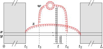
Figure 1: A Feynman graph representative for the evolution of jet quenching in the double logarithmic approximation and with a running coupling. This graphs exhibits a parton cascade made with 2 gluons successively radiated in the evolution (the gluon at $\bm{z}$ being radiated before the one at $\bm{w}$), together with a gluon loop representative of the running coupling effects. The whole cascade suffers a single scattering, at some intermediate time $t$. As suggested by this picture, successive gluons in the evolution have shorter and shorter lifetimes and larger and larger transverse sizes (which are all much larger than the size $r=|\bm{x}-\bm{y}|$ of the original dipole).

These corrections are associated with gluon fluctuations (unresolved gluon emissions with energies $\omega<\omega_{c}$) which in the plasma rest frame are naturally interpreted as bremsstrahlung by the projectile: these emissions are soft relative to their parent quark (typically, $\omega\ll\omega_{c}<E$), but hard as compared to the medium constituents ($\omega\gg 1/\lambda$). The double–logarithmic enhancement comes from integrating over the (energy and transverse) phase–space for these emissions and, more precisely, over the particular domain in this phase–space which corresponds to fluctuations which scatter only once during their formation time $\tau=2\omega/p_{\perp}^{2}$. Specifically, one logarithm is generated by integrating over $\tau$ within the range $\lambda\ll\tau\ll L$, and the other by integrating over the gluon transverse momentum $p_{\perp}$, within the range $\hat{q}\tau\ll p_{\perp}^{2}\ll Q_{s}^{2}(L)$. The lower limit $\hat{q}\tau$ on $p_{\perp}^{2}$ is the condition of single scattering and will play a major role in what follows. Gluon emissions with lower momenta $p_{\perp}^{2}\lesssim\hat{q}\tau$ are possible as well, but they undergo multiple scattering and do not contribute to double–logarithmic accuracy. (But they do contribute to single–logarithmic accuracy: they generate corrections of order $\bar{\alpha}_{s}\ln(L/\lambda)$ Liou:2013qya ; Iancu:2014kga .) Notice that gluons with energy $\omega\sim\omega_{c}(L)$ and transverse momentum $p_{\perp}\sim Q_{s}(L)$ have a formation time $\tau=L$ ; hence, $\omega_{c}$ is the upper limit on the energy of the medium–induced emissions Baier:1996kr ; Baier:1996sk ; Zakharov:1996fv .

These large one–loop corrections represent only the first step in a quantum evolution, which can be viewed as an evolution with increasing the ‘medium size’ $L$ (more precisely, the distance $L$ travelled by the projectile through the medium) for a given value of $\lambda$. Namely, the primary gluons emitted by the projectile can in turn radiate even softer gluons, thus giving rise to gluon cascades, which are enhanced by the phase–space: the powers of $\bar{\alpha}_{s}\equiv\alpha_{s}N_{c}/\pi$ associated with soft gluon emissions can be accompanied by either double, or at least single, logarithms of $L/\lambda$, depending upon the kinematics of the emissions. This evolution is generally non–linear, because of the multiple scattering between the partons in the cascades and the medium. Alternatively, the non–linear effects can be viewed as gluon saturation in the medium Iancu:2014kga (see also below).

A theoretical framework which encompasses this evolution to leading–logarithmic accuracy has been recently developed in Ref. Iancu:2014kga . The general evolution equations appear to be extremely complicated, because of the non–locality in time of the multiple scattering (the emitted gluons can scatter all the way during their propagation through the medium) and, related to that, because of the failure of the eikonal approximation for the evolution gluons. In particular, the dipole–$S$ matrix obeys a non–linear equation which can be viewed as a functional and non–local generalization of the BK equation Balitsky:1995ub ; Kovchegov:1999yj . This equation is probably too complicated to be solved in general. Fortunately though, the double–logarithmic corrections, which are the dominant corrections in the limit where $L/\lambda\gg 1$, are comparatively simple and easy to extract from the general evolution — precisely because they are associated with single scattering alone. These corrections form an ‘island’ of (effectively) linear evolution, where the non–linear effects enter only via the boundaries of the phase–space (namely, via the condition $p_{\perp}^{2}\gg\hat{q}\tau$ alluded to above). A Feynman graph representative for these corrections is illustrated in Fig. 1.

As shown in Iancu:2014kga , the linear evolution in the double logarithmic approximation (DLA) preserves the same functional form for $\mathcal{S}(\bm{r})$ as at tree–level, cf. Eq. (15), except for the replacement of the tree–level jet quenching parameter $\hat{q}^{(0)}$ by a renormalized ‘value’ (actually, a function of two variables; see below) $\hat{q}$ :

$$\mathcal{S}(L,\bm{r})\,\simeq\,\exp\left\{-\frac{1}{4}L\hat{q}(L,1/r^{2})\,\bm{r}^{2}\right\}\,.$$ (5)

In turn, this implies the universality of the evolution to this accuracy: all the quantities that can be computed from the dipole $S$–matrix ($p_{\perp}$–broadening, radiative energy loss, BDMPSZ spectrum) get renormalized simply via the appropriate redefinition of $\hat{q}$.

Eq. (5) involves the function $\hat{q}(\tau,\bm{p}^{2})$ which represents the renormalized jet quenching parameter as obtained after integrating our fluctuations with lifetimes up to $\tau$ and transverse momenta up to $\bm{p}^{2}$, the double–logarithmic accuracy. This function has support at $\bm{p}^{2}\geq\hat{q}\tau$, where it is defined as the solution to the following integral equation Liou:2013qya ; Iancu:2014kga ; Blaizot:2014bha :

$$\hat{q}(\tau,\bm{p}^{2})=\hat{q}^{(0)}+\bar{\alpha}_{s}\int_{\lambda}^{\tau}\frac{{\rm d}\tau_{1}}{\tau_{1}}\int_{\hat{q}\tau_{1}}^{\bm{p}^{2}}\frac{{\rm d}\bm{p}_{1}^{2}}{\bm{p}_{1}^{2}}\,\hat{q}(\tau_{1},\bm{p}_{1}^{2})\,,$$ (6)

to be subsequently referred to as the DLA equation with a saturation boundary. The ‘saturation boundary’ is the lower limit $\hat{q}\tau_{1}$ in the above integral over $\bm{p}_{1}^{2}$, which expresses the single–scattering condition, as already mentioned. This condition can be also understood with reference to gluon saturation in the medium Iancu:2014kga : the quantity $x\equiv\lambda/\tau$ represents the longitudinal momentum fraction of the gluons from the medium which participate in the scattering, whereas $\hat{q}\tau=\hat{q}\lambda/x\equiv Q_{s}^{2}(x)$ is the plasma saturation momentum for a given $x$. (The ‘global’ scale $Q_{s}^{2}(L)$ introduced before is the maximal possible value of $Q_{s}^{2}(x)$, corresponding to $x=x_{\rm min}\equiv\lambda/L$.) Then the condition $p_{\perp}^{2}\gg\hat{q}\tau$ can be rewritten in the more familiar form $p_{\perp}^{2}\gg Q_{s}^{2}(x)$, which defines the dilute part of the gluon distribution in the medium. Because of the presence of this saturation boundary, Eq. (6) differs from the more familiar ‘DLA equation’ encountered in studies of the BFKL or DGLAP evolutions, and this difference has profound physical consequences, as we shall see.

For our present purposes, it is more convenient to view the saturation momentum as a function of the lifetime $\tau$ of the gluon fluctuations, rather than of their longitudinal momentum fraction $x$. Given the solution $\hat{q}(\tau,\bm{p}^{2})$ to Eq. (6), the saturation momentum $Q_{s}^{2}(\tau)$ is implicitly defined by the following equation, which generalizes Eq. (3) :

$$Q_{s}^{2}(\tau)\,=\,\tau\,\hat{q}\big{(}\tau,\bm{p}^{2}=Q_{s}^{2}(\tau)\big{)}\,.$$ (7)

The value of the function $Q_{s}^{2}(\tau)$ at the ‘physical point’ $\tau=L$ determines the $p_{\perp}$–spectrum according to Eq. (4). But in order to compute the function $\hat{q}(\tau,\bm{p}^{2})$ along the saturation line $\bm{p}^{2}=Q_{s}^{2}(\tau)$, and in particular at $\tau=L$, we need to first solve the non–local equation (6) for generic values $\tau$ and $\bm{p}^{2}\geq\hat{q}\tau$.

Note also that the lower integration limit $\hat{q}\tau_{1}$ in Eq. (6) should be more precisely understood as $Q_{s}^{2}(\tau_{1})$. (The notation “$\hat{q}\tau_{1}$” becomes ambiguous when $\hat{q}$ is a non–trivial function of $\tau$ and $\bm{p}^{2}$.) Since the saturation momentum $Q_{s}^{2}(\tau)$ is itself determined by the solution to Eq. (6), cf. Eq. (7), one may wonder what should be the respective value to be used in the integration limit in Eq. (6). We shall later show that, to the desired accuracy, this can be safely taken as the initial saturation momentum, as determined by Eq. (3). Furthermore, still for that purpose, one can neglect the mild dependence of $\hat{q}^{(0)}$ upon the transverse momentum $\bm{p}^{2}$, that is, one can treat $\hat{q}^{(0)}$ as a constant within the integration limit. A similar approximation is authorized in the calculation of the renormalized saturation momentum according to Eq. (7) : to DLA accuracy, one can write $Q_{s}^{2}(\tau)=\tau\hat{q}_{s}(\tau)$ with $\hat{q}_{s}(\tau)\equiv\hat{q}(\tau,\bm{p}^{2}=\hat{q}^{(0)}\tau)$.

For what follows, it is useful to rewrite Eq. (6) in terms of the logarithmic variables $Y\equiv\ln(\tau/\lambda)$ and $\rho\equiv\ln(\bm{p}^{2}/\hat{q}^{(0)}\lambda)$. For arbitrary $Y$ and $\rho$ with $\rho\geq Y$, we have

$$\hat{q}(Y,\rho)=\hat{q}^{(0)}+\bar{\alpha}_{s}\int_{0}^{Y}{\rm d}Y_{1}\int_{Y_{1}}^{\rho}{\rm d}\rho_{1}\,\hat{q}(Y_{1},\rho_{1}).$$ (8)

Note that the tree–level saturation line $\bm{p}^{2}=\hat{q}^{(0)}\tau$ corresponds to $\rho=Y$. After evolution, this becomes $Q_{s}^{2}(Y)=\lambda{\rm e}^{Y}\hat{q}_{s}(Y)$, with $\hat{q}_{s}(Y)=\hat{q}(Y,\rho=Y)$.

One obvious question refers to the validity limits of the present approximation. Eq. (6) or (8) resums the double–logarithmic corrections, but not also the single–logarithmic ones. Hence, clearly, (i) this resummation becomes necessary when $L/\lambda$ is large enough for $\bar{\alpha}_{s}\ln^{2}(L/\lambda)\gtrsim 1$ (or $\bar{\alpha}_{s}Y^{2}\gtrsim 1$), (ii) it correctly provides the dominant asymptotic behavior in the large–medium limit $\bar{\alpha}_{s}\ln^{2}(L/\lambda)\gg 1$ (or $\bar{\alpha}_{s}Y^{2}\gg 1$), and (iii) it has an intrinsic error of relative order $\bar{\alpha}_{s}\ln(L/\lambda)$ (or $\bar{\alpha}_{s}Y$). This implies that the DLA can be strictly trusted for $Y$–values within a window

$$\frac{1}{\sqrt{\bar{\alpha}_{s}}}\ \lesssim\ Y\ <\ \frac{1}{\bar{\alpha}_{s}}\,,$$ (9)

which is parametrically large when $\bar{\alpha}_{s}\ll 1$, but in practice is admittedly quite limited. Yet, as alluded to above, the dominant asymptotic behavior of the DLA solution can be trusted for arbitrarily large $Y$. This conclusion will be substantiated by the subsequent analysis of Eq. (8), which will allow us to more precisely characterize the accuracy of the DLA in relation with the asymptotic behavior.

So far, our whole discussion has been carried at strict leading order in pQCD, meaning that the coupling $\bar{\alpha}_{s}$ in Eq. (8) is a priori fixed. But as well known from the experience with pQCD evolution, the inclusion of running coupling effects is truly essential in order to obtain realistic estimates (in particular, for applications to the phenomenology). This is particularly important for the problem at hand, in view of the strong non–locality of Eq. (8) in the transverse phase–space, which is logarithmic. The situation is reminiscent in that respect of the familiar DGLAP equation Gribov:1972ri ; Dokshitzer:1977sg ; Altarelli:1977zs and its DLA limit DeRujula:1974rf : there is no fundamental distinction between the transverse logarithms coming from the integration over the phase–space and those introduced by the running of the coupling. In that sense, the running coupling effects count already to leading order. To cope with that, we shall introduce the one–loop running of the coupling according to

$$\bar{\alpha}_{s}(\rho)=\frac{b}{\ln(\bm{p}^{2}/\Lambda^{2})}=\frac{b}{\rho+\rho_{0}}\quad\mbox{with}\quad b=\frac{12N_{c}}{11N_{c}-2N_{f}}\,.$$ (10)

Whenever we shall need a specific value, we shall chose $N_{f}=N_{c}=3$, and hence $b=4/3$. The ‘constant shift’ $\rho_{0}=\ln\big{(}\hat{q}^{(0)}\lambda/\Lambda^{2}\big{)}$ in Eq. (11) emerges from the fact that, even though $\rho$ is logarithmically related to $\bm{p}^{2}$, the reference scale is not $\Lambda^{2}$. As we shall later see, the presence of this reference scale $\rho_{0}$ is truly important for numerical estimates, in particular, for the phenomenology.

Returning to Eq. (8), it is quite clear (especially in view of the experience with the DGLAP evolution) that the proper scale for evaluating the factor $\bar{\alpha}_{s}$ is the ‘running’ scale $\rho_{1}$. This brings us to the following form for the DLA evolution equation with running coupling (RC):

$$\hat{q}(Y,\rho)=\hat{q}^{(0)}+b\int_{0}^{Y}{\rm d}Y_{1}\int_{Y_{1}}^{\rho}\frac{{\rm d}\rho_{1}}{\rho_{1}+\rho_{0}}\,\hat{q}(Y_{1},\rho_{1}).$$ (11)

III The jet quenching parameter at tree-level

In order to solve the DLA equations (8) and (11) via iterations, one needs more information about the initial condition $\hat{q}^{(0)}$, namely, one needs to know its dependence upon the resolution scale $\rho$ and also (in view of the RC problem) upon the QCD coupling. In this section, we shall briefly recall the leading order calculation of $\hat{q}^{(0)}$, with emphasis on the two aspects alluded to above. We refer to the literature for more detailed discussions Baier:1996kr ; Baier:1996sk ; Arnold:2001ms ; Arnold:2002ja ; Arnold:2008iy ; Arnold:2008vd ; CaronHuot:2008ni . At leading order, the argument of the running coupling is ambiguous and will be fixed from physical considerations. To that aim, we need to carefully keep trace of the physical origin of the various factors of $\alpha_{s}$.

As explained in the previous section, our starting point is the dipole $S$–matrix $\mathcal{S}(\bm{r})$, that we shall here evaluate at tree–level. We assume that the energy of the dipole, as measured in the rest frame of the medium, is high enough for the eikonal approximation to be applicable. In this approximation, the effect of the interaction is a color precession of the quark and the antiquark by the (fluctuating) color field representing the (gluon distribution of the) medium. Assuming the dipole to be a right–mover, and hence the medium to be a left–mover, the dipole $S$–matrix is computed as

$$\mathcal{S}(\bm{x},\bm{y})\,=\,\frac{1}{N_{c}}\,\Big{\langle}{\rm tr}\big{[}V^{\dagger}({\bm{x}}){V}({\bm{y}})\big{]}\Big{\rangle}\,,\qquad V^{\dagger}(\bm{x})={\rm P}\exp\left\{{\rm i}g\int{\rm d}x^{+}\,A^{-}_{a}(x^{+},{\bm{x}})t^{a}\right\}\,.$$ (12)

Here $\bm{x}$ and $\bm{y}$ are the transverse coordinates of the quark, respectively, the antiquark, which are not changed by the interaction, $V^{\dagger}({\bm{x}})$ and ${V}({\bm{y}})$ are Wilson lines describing the respective color precessions, $A^{-}_{a}(x^{+},{\bm{x}})$ is the ‘large’ component of the color field in the target, which is randomly distributed (due to quantum and thermal fluctuations), and the brackets $\langle\cdots\rangle$ refer to the average over this ‘background’ field. The light–cone coordinate $x^{+}\equiv(x^{0}+x^{3})/\sqrt{2}$ plays the role of a ‘time’ for the dipole and, respectively, of a longitudinal coordinate for the medium. The $t^{a}$’s are the color group generators in the fundamental representation and P stands for path ordering w.r.t. $x^{+}$.

A weakly–coupled medium can be described as a collection of independent color charges — thermal quarks and gluons for a QGP with sufficiently high temperature $T$, or valence quarks for dense CNM, as described in the McLerran–Venugopalan (MV) model McLerran:1993ni ; McLerran:1994vd . These charges will be assumed to be point–like and have no other mutual interactions, except for those responsible for the screening of the color interactions over a transverse distance $r\sim 1/\Lambda$. For a weakly–coupled QGP, this screening is perturbative and $\Lambda=m_{D}$, with $m_{D}^{2}\sim\bar{\alpha}_{s}T^{2}$ the Debye mass. Here, however, we shall mostly focus on the case of CNM, where the screening is non–perturbative and associated with confinement. Under these assumptions, the only non–trivial correlator of the target field $A^{-}$ is the respective 2–point function, which has the following structure

$$\left\langle A^{-}_{a}(x^{+},x^{-},\bm{x})\,A^{-}_{b}(y^{+},y^{-},\bm{y})\right\rangle\,=\,\delta_{ab}\delta(x^{+}-y^{+})\,n_{0}\gamma(\bm{x}-\bm{y})\,,$$ (13)

where $n_{0}$ is the number density of the medium constituents, weighted with appropriate color factors. For simplicity we assume the medium to be homogeneous. Also

$$\gamma(\bm{k})\equiv\int{\rm d}^{2}\bm{r}\ {\rm e}^{{\rm i}\bm{k}\cdot\bm{r}}\,\gamma(\bm{r})\,\simeq\,\frac{g^{2}}{\bm{k}^{4}}\,,$$ (14)

(with the approximate equality holding for $k_{\perp}\gg\Lambda$) is the square of the 2–dimensional Coulomb propagator. It is understood that Eq. (14) must be used with an infrared cutoff $k_{\perp}\simeq\Lambda$.

For the Gaussian field distribution in Eq. (13), it is a straightforward exercise to compute the average $S$–matrix for a quark–antiquark dipole. One finds (with $\bm{r}\equiv\bm{x}-\bm{y}$)

$$\mathcal{S}^{(0)}(\bm{r})\,=\,\exp\Biggl{\{}-g^{2}C_{F}n_{0}L\int\frac{{\rm d}^{2}\bm{k}}{(2\pi)^{2}}\,\gamma(\bm{k})\left(1-{\rm e}^{{\rm i}\bm{k}\,\cdot\,\bm{r}}\right)\Biggr{\}}\,.$$ (15)

Using Eq. (14), one sees that the integral over $\bm{k}$ in Eq. (15) is logarithmically sensitive to the IR cutoff $\Lambda$. We shall be mostly interested in small dipole sizes $r\equiv|\bm{r}|\ll 1/\Lambda$. Then, there is a large logarithmic phase–space, at $\Lambda\ll k_{\perp}\ll 1/r$. To leading logarithmic accuracy, the integral can be evaluated by expanding the complex exponential ${\rm e}^{{\rm i}\bm{k}\,\cdot\,\bm{r}}$ to second order (the linear term vanishes after angular integration). One thus finds the result previously shown in Eq. (15), with the following expression for $\hat{q}^{(0)}(Q^{2})$ (we recall that $Q^{2}=1/r^{2}\gg\Lambda^{2}$) :

$$\hat{q}^{(0)}(Q^{2})\,\simeq\,4\pi\alpha_{s}(Q^{2})C_{F}n_{0}\int^{Q^{2}}_{\Lambda^{2}}\frac{{\rm d}\bm{k}^{2}}{\bm{k}^{2}}\,\alpha_{s}(\bm{k}^{2})\,\sim\,\alpha_{s}(Q^{2})\,n_{0}\,xG(x,Q^{2})\,.$$ (16)

This is the tree–level jet quenching parameter for an incoming quark. The corresponding quantity for a gluon is obtained by multiplying Eq. (16) with $N_{c}/C_{F}$. As also shown above, this expression is usually written as a proportionality between $\hat{q}^{(0)}(Q^{2})$ and the gluon distribution $xG(x,Q^{2})$ produced by one parton in the medium, on the resolution scale $Q^{2}$.

In writing Eq. (16), we have already ascribed the running scales for each of the two factors of $\alpha_{s}$, on physical grounds: (i) The factor $\alpha_{s}$ outside the integral originates in the coupling between the (anti)quark in the dipole and the target color field, via the Wilson lines in Eq. (12); the transverse resolution for this interaction is fixed by the dipole size, $Q^{2}=1/r^{2}$, so this is the natural argument for the running of that coupling. (ii) The factor $\alpha_{s}$ inside the integral comes from the Coulomb propagator (14), so it naturally runs with the momentum $k_{\perp}^{2}$ exchanged via Coulomb scattering.

In the case of a fixed coupling, the integral over $\bm{k}^{2}$ generates a logarithmic enhancement:

$$\hat{q}^{(0)}(Q^{2})\,\simeq\,4\pi\alpha_{s}^{2}C_{F}n_{0}\ln\frac{Q^{2}}{\Lambda^{2}}\qquad\mbox{(fixed coupling)}\,.$$ (17)

On the other hand, with a running coupling, the integral over $\bm{k}^{2}$ yields only a mild enhancement:

$$\hat{q}^{(0)}(Q^{2})\,\simeq\,4\pi\alpha_{s}(Q^{2})C_{F}n_{0}b_{0}\ln{\ln({Q^{2}}/{\Lambda^{2}})}\qquad\mbox{(running coupling)}\,,$$ (18)

where $b_{0}$ is related to the parameter $b$ introduced in Eq. (10) via $b=(N_{c}/\pi)b_{0}$.

One can summarize the above results as follows:

$$\hat{q}^{(0)}(\rho)=\begin{cases}\tilde{q}^{(0)}(\rho+\rho_{0})&\mbox{for fixed coupling},\\[5.69046pt] \tilde{q}^{(0)}\displaystyle{\frac{\ln(\rho+\rho_{0})}{\rho+\rho_{0}}}&\mbox{for running coupling}.\end{cases}$$ (19)

where $\rho=\ln(Q^{2}/\hat{q}^{(0)}\lambda)$, $\rho_{0}=\ln(\hat{q}^{(0)}\lambda/\Lambda^{2})$, and it is understood that the $\rho$–independent prefactor $\tilde{q}^{(0)}$ is different for fixed and respectively running coupling, although we shall use the same notation in both cases.

In what follows, we shall study the DLA solutions with the initial conditions given by Eq. (19), and also those where $\hat{q}^{(0)}$ is taken to be simply a constant. The latter choice allows for simpler analytic manipulations, while yielding the same asymptotic behavior at large $Y=\rho$ — for both fixed and running coupling — as the more ‘realistic’ initial conditions in Eq. (19). This points out towards the universality of the large–$Y$ asymptotics w.r.t. the choice of the initial conditions.

IV The exact solution for fixed coupling

It turns out that it is rather straightforward to solve the fixed coupling evolution equation (8) via successive iterations. For a constant (i.e. $\rho$–independent) initial condition and on the (tree–level) saturation line $\rho=Y$, the corresponding solution — to be denoted here as $\hat{q}_{s}(Y)$ — has already been constructed in this in Ref. Liou:2013qya . In this section we shall extend the solution in Liou:2013qya to generic values of $\rho$ and also to the more realistic, $\rho$–dependent, initial condition shown in the first line of Eq. (19).

For reasons to shortly become clear, it is convenient to perform the $\rho_{1}$–integration in Eq. (8) in the full available space, that is from 0 to $\rho$, and then subtract the contribution which is cut by the saturation boundary. That is, we shall write one iteration step as

$$\hat{q}^{(n)}(Y,\rho)=\bar{\alpha}_{s}\int_{0}^{Y}{\rm d}Y_{1}\int_{0}^{\rho}{\rm d}\rho_{1}\,\hat{q}^{(n-1)}(Y_{1},\rho_{1})-\bar{\alpha}_{s}\int_{0}^{Y}{\rm d}Y_{1}\int_{0}^{Y_{1}}{\rm d}\rho_{1}\,\hat{q}^{(n-1)}(Y_{1},\rho_{1}),$$ (20)

and then the final solution will be given by the summation of the series

$$\hat{q}(Y,\rho)=\sum_{n=0}^{\infty}\hat{q}^{(n)}(Y,\rho).$$ (21)

Our notation is such that $\hat{q}^{(n)}$ is the correction of order $\bar{\alpha}_{s}^{n}$. Assuming a momentum independent initial condition $\hat{q}^{(0)}$, it is trivial to do the first iteration and find

$$\hat{q}^{(1)}(Y,\rho)=\hat{q}^{(0)}\bar{\alpha}_{s}Y\rho-\hat{q}^{(0)}\bar{\alpha}_{s}\,\frac{Y^{2}}{2},$$ (22)

where the two terms correspond to the two terms in Eq. (20). Proceeding to the second iteration one may naively expect that there will be four terms, however one finds the that two terms generated by inserting Eq. (22) into the ‘subtracted’ contribution in Eq. (20) exactly cancel each other. Remarkably, this pattern repeats itself to all subsequent orders in $\bar{\alpha}_{s}^{n}$ ; that is, only the first term in Eq. (20) contributes to the calculation of $\hat{q}^{(n)}(Y,\rho)$ for $n\geq 2$. It is then straightforward to deduce that for a generic $n$ one has

$$\hat{q}^{(n)}(Y,\rho)=\hat{q}^{(0)}\,\frac{(\bar{\alpha}_{s}Y\rho)^{n}}{(n!)^{2}}-\hat{q}^{(0)}(1-\delta_{n0})\,\frac{Y}{\rho}\,\frac{(\bar{\alpha}_{s}Y\rho)^{n}}{(n-1)!(n+1)!},$$ (23)

where the factor $1-\delta_{n0}$ removes the second term when $n=0$. The two terms above are easily recognized as belonging to the Taylor expansions of two modified Bessel functions of the first kind, ${\rm I}_{0}$ and respectively ${\rm I}_{2}$ :

$$\hat{q}(Y,\rho)=\hat{q}^{(0)}\bigg{[}{\rm I}_{0}\big{(}2\sqrt{\bar{\alpha}_{s}Y\rho}\big{)}-\frac{Y}{\rho}\,{\rm I}_{2}\big{(}2\sqrt{\bar{\alpha}_{s}Y\rho}\big{)}\bigg{]}.$$ (24)

By itself, the first term alone would be the solution to the standard DLA equation, which has no saturation boundary DeRujula:1974rf ; Kovchegov:2012mbw ; that is, this is the solution that would be obtained by iterating the first term in the r.h.s. of Eq. (20) alone. Vice–versa, the second, negative, term in Eq. (24) is entirely due to the presence of the saturation boundary and is reminiscent of a corresponding term emerging in the calculation of the saturation momentum for a ‘shockwave’ (a Lorentz contracted, large, nucleus) Mueller:2002zm . In that case too, the evolution of the dipole $S$–matrix in the vicinity of the saturation line can be approximately described by a linear equation with a saturation boundary, but the respective linear equation is BFKL Lipatov:1976zz ; Kuraev:1977fs ; Balitsky:1978ic (the linearized version of BK equation), and not DLA.

The asymptotic expansion of the modified Bessel function ${\rm I}_{n}(x)$ for large values of its argument $x$ reads

$${\rm I}_{n}(x)=\frac{{\rm e}^{x}}{\sqrt{2\pi x}}\bigg{(}1+\frac{1-4n^{2}}{8x}+\cdots\bigg{)}.$$ (25)

That is, both the leading exponential behavior and the leading term in the prefactor are independent of $n$. This implies that the dominant exponential behavior of the solution (24) for large values of $x=2\sqrt{\bar{\alpha}_{s}Y\rho}$ is the same as it would be in the absence of the boundary. Most likely, this feature has no fundamental meaning since, as we shall later discover, it is in fact washed out by the running of the coupling.

When evaluating Eq. (24) on the (tree–level) saturation line at $\rho=Y$, the leading order term in the asymptotic expansion at large $x=2\sqrt{\bar{\alpha}_{s}}\,Y$ (the unity within the brackets in Eq. (25)) precisely cancels between the two terms in Eq. (24). Accordingly, the suppression due to the boundary manifests itself at large $Y$ as an additional $1/Y$ prefactor. Again, this is similar to the corresponding problem for a shockwave, as controlled by the BFKL equation with a saturation boundary: in that case too, the boundary introduces an extra prefactor $1/Y$ in the dominant behavior of the dipole amplitude at large $Y$ and in the vicinity of the saturation line Mueller:2002zm .

As a matter of facts, for $\rho=Y$ one can combine the two terms in Eq. (24) to get a rather compact expression (the second equality below holds for $Y\gg 1/\sqrt{\bar{\alpha}_{s}}$),

$$\hat{q}_{s}(Y)=\hat{q}^{(0)}\,\frac{{\rm I}_{1}\big{(}2\sqrt{\bar{\alpha}_{s}}\,Y\big{)}}{\sqrt{\bar{\alpha}_{s}}\,Y}=\hat{q}^{(0)}\,\frac{{\rm e}^{2\sqrt{\bar{\alpha}_{s}}\,Y}}{\sqrt{4\pi}\,(\sqrt{\bar{\alpha}_{s}}Y)^{3/2}}\left[1+\mathcal{O}(1/\sqrt{\bar{\alpha}_{s}}Y)\right],$$ (26)

which agrees with the corresponding result in Ref. Liou:2013qya . The additional prefactor $1/\sqrt{\bar{\alpha}_{s}}\,Y$ is manifest on Eq. (26). The renormalized saturation momentum is then obtained as

$$Q_{s}^{2}(Y)=\lambda\hat{q}_{s}(Y){\rm e}^{Y}\simeq\,Q_{s}^{2}(0)\,\frac{{\rm e}^{(1+2\sqrt{\bar{\alpha}_{s}})Y}}{\sqrt{4\pi}\,(\sqrt{\bar{\alpha}_{s}}Y)^{3/2}}\,,$$ (27)

which shows that $\gamma_{s}\equiv 2\sqrt{\bar{\alpha}_{s}}$ plays the role of an ‘anomalous’ saturation exponent within the fixed coupling scenario.

So far, we have used the tree–level definition of the saturation line, $\bm{p}^{2}=\hat{q}^{(0)}\tau$ or $\rho=Y$, both in the integration limit in Eq. (6) and in the calculation of the saturation momentum in Eq. (27). As discussed in relation with Eq. (7), this choice is ambiguous and the sensitivity of the results to this ambiguity may be viewed as an indication of our error. To estimate this error, we can, for example, change the lower limit in each iteration with the updated value of $\hat{q}$, or even with the resummed value given in Eq. (26). Both prescriptions lead to a correction of the same order, so let us follow the second one, since it is rather easy to implement. Keeping only the leading asymptotic behavior of $\hat{q}_{s}(Y)$, as given by the exponential in Eq. (26), we see that the lower limit of the $\rho_{1}$ integration in Eq. (8) changes from $Y_{1}$ to $(1+2\sqrt{\bar{\alpha}_{s}})Y_{1}$. Then it is an easy exercise to show that Eq. (24) gets replaced by

$$\hat{q}(Y,\rho)=\hat{q}^{(0)}\bigg{[}{\rm I}_{0}\big{(}2\sqrt{\bar{\alpha}_{s}Y\rho}\big{)}-\frac{Y}{\rho}\,(1+2\sqrt{\bar{\alpha}_{s}})\,{\rm I}_{2}\big{(}2\sqrt{\bar{\alpha}_{s}Y\rho}\big{)}\bigg{]},$$ (28)

For consistency, when evaluating this expression on the saturation line, one should now use $\rho=\rho_{s}(Y)$, with $\rho_{s}(Y)\equiv(1+2\sqrt{\bar{\alpha}_{s}})Y$ (cf. Eq. (27)). Then the leading terms in the asymptotic expansion cancel again between the two terms in Eq. (28) and the net result at large $Y$ is similar to that in Eq. (26), except for the replacement of the exponential there by

$${\rm e}^{2Y\sqrt{\bar{\alpha}_{s}(1+2\sqrt{\bar{\alpha}_{s}})}}\,\simeq\,{\rm e}^{2\sqrt{\bar{\alpha}_{s}}\,Y(1+\sqrt{\bar{\alpha}_{s}})}\,=\,{\rm e}^{2\sqrt{\bar{\alpha}_{s}}\,Y}\,{\rm e}^{2\bar{\alpha}_{s}Y}\,,$$ (29)

where we have also used $\sqrt{\bar{\alpha}_{s}}\ll 1$. As compared to Eq. (26), the exponent in Eq. (29) includes an additional contribution $2\bar{\alpha}_{s}Y$, due to the change in the slope of the saturation line. This new contribution represents a perturbative correction of $\mathcal{O}{(\sqrt{\bar{\alpha}_{s}})}$ to the exponent, so the leading, exponential, behavior at large $Y$ is not modified. But if one is interested in $\hat{q}_{s}(Y)$ itself, and not only in its logarithm, then this additional piece in the exponent matters to $\mathcal{O}{(1)}$ for any $Y\gtrsim 1/\bar{\alpha}_{s}$. In other terms, the prefactor of the leading exponential is unambiguously given by our current approximations only so far as $\bar{\alpha}_{s}Y\ll 1$. This is in agreement with the fact that, by working in the DLA, the single–logarithmic contributions have been systematically neglected. We conclude that the DLA is an accurate approximation for $\hat{q}_{s}(Y)$ only within the window (9), but a good approximation for $\ln\hat{q}_{s}(Y)$ for arbitrary $Y\gtrsim 1/\sqrt{\bar{\alpha}_{s}}$.

It is quite straightforward to generalize the previous discussion to the $\rho$–dependent initial condition Then the pattern described below Eq. (22) is still present and one similarly finds

$$\hat{q}(Y,\rho)=\tilde{q}^{(0)}\frac{\rho}{\sqrt{\bar{\alpha}_{s}Y\rho}}\bigg{[}{\rm I}_{1}\big{(}2\sqrt{\bar{\alpha}_{s}Y\rho}\big{)}-\frac{Y^{2}}{\rho^{2}}\,{\rm I}_{3}\big{(}2\sqrt{\bar{\alpha}_{s}Y\rho}\big{)}\bigg{]}.$$ (30)

For $\rho=Y$, one can combine the two terms in the above to get

$$\hat{q}(Y)=\tilde{q}^{(0)}\,\frac{2\,{\rm I}_{2}\big{(}2\sqrt{\bar{\alpha}_{s}}\,Y\big{)}}{\bar{\alpha}_{s}Y}=\tilde{q}^{(0)}\,\frac{2{\rm e}^{2\sqrt{\bar{\alpha}_{s}}\,Y}}{\sqrt{4\pi\bar{\alpha}_{s}}\,(\sqrt{\bar{\alpha}_{s}}Y)^{3/2}}\left[1+\mathcal{O}(1/\sqrt{\bar{\alpha}_{s}}Y)\right],$$ (31)

where the second equality is valid in the limit $Y\gg 1/\sqrt{\bar{\alpha}_{s}}$. Comparing Eqs. (26) and (31), we see that the $Y$–dependence of the asymptotic solution (including the leading prefactor) is not altered due to the change in the initial condition.

V The asymptotic solution with running coupling

In exact analogy to the fixed coupling case, we can construct a formal solution to the running coupling equation (11) via successive iterations. This allows us to express the solution $\hat{q}(Y,\rho)$ as an infinite series, similar to Eq. (21), where however the individual terms with $n\geq 1$ are considerably more complicated than for fixed coupling. For not too large values of $n$, these terms can be efficiently computed with the help of symbolic, computer–assisted, manipulations. This is possible because the kernel in the integral equation (11) is simple enough to analytically perform the integrations, at each step in the iteration procedure. However, we shall not be able to deduce the analytic form of these terms for arbitrary values of $n$ and even less to explicitly resum the whole series. Still, through a semi–numerical procedure to be later described, we will be able to deduce the asymptotic behavior of the series at large $Y$. As we shall also demonstrate, this dominant behavior is universal within the class of initial conditions of interest. So, before we consider the more realistic initial condition in Eq. (19), let us first assume the simple scenario in which $\hat{q}^{(0)}$ is momentum independent. Since here we are primarily interested in the asymptotic expansion, we can neglect $\rho_{0}$ in the denominator of the running coupling in Eq. (11). (This assumption will be relaxed in the numerical estimates in the following section.) We then successively find

$$\hat{q}^{(1)}(Y,\rho)=\hat{q}^{(0)}bY\left(\ln\frac{\rho}{Y}+1\right),$$ (32)

$$\hat{q}^{(2)}(Y,\rho)=\hat{q}^{(0)}(bY)^{2}\left(\frac{1}{4}\ln^{2}\frac{\rho}{Y}+\frac{3}{4}\ln\frac{\rho}{Y}+\frac{3}{8}\right),$$ (33)

$$\hat{q}^{(3)}(Y,\rho)=\hat{q}^{(0)}(bY)^{3}\left(\frac{1}{36}\ln^{3}\frac{\rho}{Y}+\frac{11}{72}\,\ln^{2}\frac{\rho}{Y}+\frac{49}{216}\ln\frac{\rho}{Y}+\frac{49}{648}\right),$$ (34)

$$\cdots,$$

$$\hat{q}^{(n)}(Y,\rho)=\hat{q}^{(0)}(bY)^{n}\left[\frac{1}{(n!)^{2}}\ln^{n}\frac{\rho}{Y}+c_{n,n-1}\,\ln^{n-1}\frac{\rho}{Y}+\cdots+nc_{n,0}\ln\frac{\rho}{Y}+c_{n,0}\right].$$ (35)

A few observations are in order here. If there was not for the $Y$–dependent ‘saturation boundary’ (the lower limit $Y_{1}$ in the integral over $\rho_{1}$ in Eq. (11)), we would have to introduce an infrared cutoff at $\rho_{0}$ (or, equivalently, restore the ‘shift’ $\rho_{0}$ in the denominator of the running coupling), in order to avoid infrared singularities. Then one would easily find that, for a given $n$, only the term with the highest power $\ln^{n}(\rho/\rho_{0})$ appears. As shown in the above equation, the respective coefficient reads $c_{n,n}={1}/{(n!)^{2}}$. The corresponding series is straightforwardly resummed, since recognized as the Taylor expansion of the function ${\rm I}_{0}(x)$ with $x=2\sqrt{\,bY\ln(\rho/\rho_{0})}$. This is indeed the expected solution for the standard DLA equation with running coupling DeRujula:1974rf ; Kovchegov:2012mbw .

However, the presence of the saturation boundary significantly modifies the problem, even more than in the case of a fixed coupling. For a given $n$, we have to sum a polynomial of order $n$ in $\ln(\rho/Y)$ whose coefficients, in general, do not seem to be given by a simple analytic formula. As explicitly shown in Eq. (35) we have been able to find only the coefficient of the leading term and the ratio, equal to $n$, of the linear and constant terms. We shall come later to a discussion of the information that we can infer from this last, simple, relation.

Consider now the value of this series along the (tree–level) saturation line, $\rho=Y$. Then, for any $n$, we are left with only the constant term of the respective polynomial, namely

$$\hat{q}_{s}(Y)=\hat{q}^{(0)}\sum_{n=0}^{\infty}c_{n}(bY)^{n},$$ (36)

where we have written $c_{n}\equiv c_{n,0}$. The fact that all the logarithmic terms within the polynomial $\hat{q}^{(n)}(Y,\rho)$ cancel for $\rho=Y$ implies that the asymptotic behavior of the quantity $\hat{q}_{s}(Y)$ at large $Y$ should be very different from that of the standard DLA solution (with RC), and also much more difficult to obtain. Indeed, as suggested by the first three iterations given explicitly above, it seems difficult to find a general analytic expression for the coefficients $c_{n}$, valid for arbitrary $n$. Nevertheless, one can explicitly construct these coefficients up to very high orders, via iterations, by using a suitable mathematical program for symbolic manipulations. Then, as we shall see in a moment, the dominant behavior at large $n$ is $c_{n}\propto 1/(n!)^{2}$ (as for the evolution at fixed coupling). This in particular implies that, for a given $Y$, we only need a finite number of terms to reliably calculate $\hat{q}_{s}(Y)$ terms (cf. Eq. (42) below). More precisely, we shall argue that we need about $n\sim 2\sqrt{bY}$ terms. Vice versa, by keeping $n$ terms in the series, one can reliably calculate $\hat{q}_{s}(Y)$ up to rapidities $Y\sim n^{2}/4b$. In practice, one can easily check where to stop by requiring that adding an extra term in the series does not change the result for $\hat{q}_{s}(Y)$, to the desired accuracy.

This discussion shows that, for any given $Y$, one can accurately compute the solution $\hat{q}_{s}(Y)$ by considering only a finite truncation of the series, whose coefficients are analytically known. This being said, it would be appealing to have a closed form of $\hat{q}_{s}(Y)$ in terms of known functions. As we now explain, this becomes feasible at sufficiently large $Y$. Namely, by numerically fitting the ‘$Y$–data’, that is, the numerical values of $\hat{q}_{s}(Y)$ obtained from the properly truncated series for large values of $Y$, we have found the following asymptotic expansion:

$$\frac{{\rm d}\ln\hat{q}_{s}(Y)}{b{\rm d}Y}=\frac{2}{\sqrt{bY}}-\frac{2^{1/6}|\xi_{1}|}{(2bY)^{5/6}}+\frac{1}{4bY}+\mathcal{O}\big{(}Y^{-7/6}\big{)},$$ (37)

where $\xi_{1}=-2.338\dots$ is the rightmost zero of the Airy function. Via numerical tests, we have checked that the form of Eq. (37), including all the shown coefficients, is very robust: any tiny variation will not lead to a well–defined asymptotic series in which the remainder, here the final term of $\mathcal{O}\big{(}Y^{-7/6}\big{)}$, remains smaller in magnitude than the leading terms.

A heuristic, yet suggestive, way to understand the dominant term in Eq. (37) (including its coefficient) is as follows: keeping only this leading term, one can rewrite Eq. (37) as

$$\frac{{\rm d}\ln\hat{q}_{s}(Y)}{{\rm d}Y}=2\sqrt{\bar{\alpha}_{s}(Y)}+\cdots.$$ (38)

This is formally identical to the corresponding fixed coupling result, as extracted from Eq. (26), and with the coupling in the latter evaluated at $\rho=Y$ (the natural scale indeed). A similar relation between the asymptotic behaviors at fixed and respectively running coupling has also been observed in the case of a shockwave Iancu:2002tr ; Mueller:2002zm . Perhaps even more remarkable, and also quite intriguing, this resemblance with the corresponding shockwave problem extends to the second term in the asymptotic expansion (37), i.e. the first preasymptotic term $\propto Y^{-5/6}$. Indeed, exactly the same term appears in the asymptotic expansion of the logarithmic derivative of the saturation momentum ${\rm d}\ln Q_{s}^{2}(Y)/{\rm d}Y$ as obtained from the BK equation (or from the BFKL equation with a saturation boundary) Mueller:2002zm ; Munier:2003sj . In fact, it was this observation that has led us to ‘guess’ the form of this particular term when trying to fit the $Y$–data. We shall comment in a while on the origin of the last term $\propto 1/Y$ in Eq. (37).

The terms given in Eq. (37) are sufficient, modulo a constant arising from the integration, to determine the asymptotic behavior of the jet quenching parameter at large $Y$ :

$$\ln\hat{q}_{s}(Y)\,=\,4{\sqrt{bY}}-{3|\xi_{1}|}{(4bY)^{1/6}}+\frac{1}{4}\ln Y+\kappa+\mathcal{O}\big{(}Y^{-1/6}\big{)}\,.$$ (39)

We have numerically evaluated the additional constant term $\kappa$ in the asymptotic expansion of $\ln\hat{q}_{s}(Y)$ and found it to be close to 5.7. When exponentiated, this leads to a unnaturally large multiplicative coefficient, close to 300, in the expression for $\hat{q}_{s}(Y)$. This large factor finds its origin in the fact that we have neglected the constant $\rho_{0}$ when performing the transverse momentum integrations. Indeed, although these integrations are finite as they stand, there are strongly sensitivity to the lowest momenta (where the coupling is stronger), thus generating very large contributions. As we shall verify in the next section, the inclusion of a realistic value for $\rho_{0}$ strongly suppresses the magnitude of the solution $\hat{q}_{s}(Y)$, while leaving unchanged the asymptotic behavior (37) of the derivative of $\ln\hat{q}_{s}(Y)$.

Eq. (39) also shows that, with running coupling, the medium saturation momentum has the following dominant exponential behavior at large $Y$ :

$$Q_{s}^{2}(Y)\,\propto\,{\rm e}^{Y+4\sqrt{bY}}\,.$$ (40)

As compared to the fixed coupling scenario, cf. Eq. (27), the effects of the radiative corrections are now milder: there is no ‘anomalous’ contribution to the saturation exponent anymore, just a correction to $\ln Q_{s}^{2}(Y)$ which grows like $\sqrt{Y}$. This is very similar to what happens in the case of a shockwave Iancu:2002tr ; Mueller:2002zm ; Munier:2003sj .

It is also useful to mention that one can equivalently fit the $n$–data, that is the coefficients $c_{n}$ in the expansion Eq. (36). In such an approach one finds, for large $n$,

$$c_{n}=\tilde{\kappa}\,\frac{4^{n}{\rm e}^{-3|\xi_{1}|n^{1/3}}}{(n-1)!n!},$$ (41)

where the proportionality factor is related to the constant $\kappa$ introduced in Eq. (39) via $\tilde{\kappa}=\sqrt{2\pi}{\rm e}^{\kappa}$ and can be numerically determined. Then, one can convert the summation in Eq. (36) into an integration which can be done by the steepest–descent method. For a given $Y$, the integrand is dominated by values of $n$ around

$$n_{c}=2\sqrt{bY}-\frac{|\xi_{1}|(4bY)^{1/6}}{2}.$$ (42)

This result justifies our previous statement concerning the numbers of terms needed in order to give an accurate result for the jet quenching parameter for a given $Y$. Moreover, one can see that the Gaussian integration around the saddle point $n_{c}$ leads to a prefactor proportional to $Y^{1/4}$ which in turn explains the third term in the expansion in equation (37).

As in the fixed coupling scenario, the full asymptotic expansion given in Eq. (37) does not seem to depend on the initial condition. We have found that Eq. (37) remains valid when we consider either the initial condition of Eq. (19), or a similar one in which the logarithm in the numerator is absent.

Finally, we can get some information regarding the $\rho$–dependence of the two–variable function $\hat{q}(Y,\rho)$ for values of $\rho$ not too far from the saturation boundary. In this regime it is sufficient to add to the previous result only the term linear in $\ln(\rho/Y)$. This is rather easy to achieve, since the coefficients of the $\ln(\rho/Y)$ terms are related to those of the constant terms by just a factor of $n$ (cf. Eq. (35)). The analog of Eq. (21) becomes

$$\hat{q}(Y,\rho)=\hat{q}^{(0)}\sum_{n=0}^{\infty}c_{n}(bY)^{n}+\ln\frac{\rho}{Y}\,\hat{q}^{(0)}\sum_{n=1}^{\infty}n\,c_{n}(bY)^{n}+\cdots,$$ (43)

where the dots stand for terms of higher order in $\ln(\rho/Y)$. Notice that to the order of accuracy one has that $\ln(\rho/Y)\simeq(\rho-Y)/Y$. It is trivial to see that the second term in Eq. (43) can be expressed in terms of the $Y$–derivative of the first term [which is the quantity that we have called $\hat{q}_{s}(Y)$], so that

$$\hat{q}(Y,\rho)\simeq\hat{q}_{s}(Y)+(\rho-Y)\frac{{\rm d}\hat{q}_{s}(Y)}{{\rm d}Y}\simeq\left(1+\frac{2(\rho-Y)\sqrt{b}}{\sqrt{Y}}\right)\hat{q}_{s}(Y).$$ (44)

The first equality in the above is general (it holds for both fixed or running coupling) : this is the beginning of the Taylor expansion of $\hat{q}(Y,\rho)$ near $\rho=Y$. Indeed, by inspection of the integration limits in Eqs. (8) and (11), one can verify that

$$\frac{\partial\hat{q}(Y,\rho)}{\partial Y}\Big{|}_{\rho=Y}=0\quad\Longrightarrow\quad\frac{\partial\hat{q}(Y,\rho)}{\partial\rho}\Big{|}_{\rho=Y}=\frac{{\rm d}\hat{q}_{s}(Y)}{{\rm d}Y}\,.$$ (45)

For the second equality in Eq. (44), we have used the leading asymptotic term in Eq. (37) (or, equivalently, Eq. (38)). The expansion in Eq. (43) is valid so long as the second term, linear in the separation $\rho-Y$ from the saturation boundary, remains much smaller than the first one. For the running coupling case, this is the case provided $\rho-Y\lesssim\sqrt{Y/b}\sim{1/\sqrt{\bar{\alpha}_{s}(Y)}}$, which leaves us with a parametrically large window in which the $\rho$–dependence is indeed under control.

VI Numerical studies and non–universal aspects

In the previous sections, we have mostly focused on universal aspects of the evolution, like the asymptotic behavior of the (renormalized) jet quenching parameter $\hat{q}_{s}(Y)$ for large values of $Y$, which are insensitive to the details of the initial condition $\hat{q}^{(0)}$, such as the constant shift $\rho_{0}$ in the momentum variable $\rho$ in Eq. (19). This has enabled us to analytically perform the energy ($Y$) and momentum ($\rho$) integrations in the successive iterations of the evolution equation. In the case of a fixed coupling, this permitted us to deduce exact solutions for two different initial conditions, cf. Eqs. (24) and (30). In the running coupling case, the corresponding analysis allowed us to accurately determine (via a numerical fit to the truncated series obtained via iterations) the asymptotic behavior of $\ln\hat{q}_{s}(Y)$, up to terms which die away as $Y\to\infty$, cf. Eq. (39).

However, some interesting questions are left unanswered by the previous analysis, among which, how fast is the approach towards asymptotics, what are the physical consequences of the shift $\rho_{0}$, and what is the net effect of the quantum evolution (say, as measured by the enhancement factor $\hat{q}_{s}(Y)/\hat{q}^{(0)}$) for phenomenologically relevant values of $Y$ and $\rho_{0}$. In this section, we shall try and answer such questions via semi–numerical studies, based on appropriate truncations of the iterative series in which the individual terms are computed analytically, but with the help of computer–assisted symbolic manipulations. Such manipulations become more tedious when $\rho_{0}\neq 0$, which limits the number of terms in the series that can be efficiently computed in that case. It is therefore important to have a good control of the convergency of the truncated series (for a given value of $Y$). This will be first tested in the case of a fixed coupling, where it is possible to compare with the exact respective results.

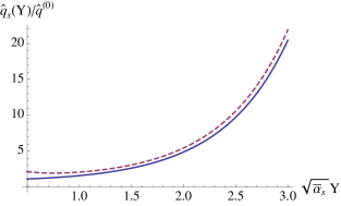
(a)

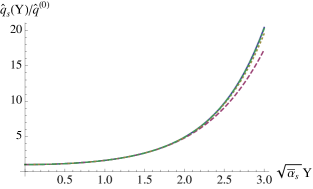
(b)

Figure 2: The jet quenching parameter $\hat{q}_{s}(Y)$, normalized to its tree level value $\hat{q}^{(0)}$, as a function of $\sqrt{\bar{\alpha}_{s}}Y$ for fixed coupling evolution and a $\rho$–independent initial condition. (a) Continuous blue: exact solution. Dashed magenta: asymptotic solution. (b) Continuous blue: exact solution. Dashed magenta, dotted gold, dotted–dashed green: truncated solutions with $n=3,4,5$ terms added to the tree level. The last curve, for $n=5$, cannot be distinguished from the exact solution.

For definiteness, we consider the $\rho$–independent initial condition, for which the exact solution with fixed coupling and its asymptotic expansion are both shown in Eq. (26). In Fig. 2.a we show a comparison between the exact and the (leading) asymptotic solution, for various values of the evolution ‘time’ $\sqrt{\bar{\alpha}_{s}}Y$. As clear from this figure, the agreement is very good down to values $\sqrt{\bar{\alpha}_{s}}Y\simeq 1$. Then, we study the convergency of the truncated series. We would like to estimate the maximum value of $Y$ up to which such a truncated solution will be trustworthy. Via analytic considerations, similar to those presented in the context of a running coupling (cf. Eq. (42)), one finds that the summation is dominated by values of $n$ around $n_{c}\sim\sqrt{\bar{\alpha}_{s}}Y$. Thus, it is not surprising that the $n=4$ truncated solution is in good agreement with the exact one up to values $\sqrt{\bar{\alpha}_{s}}Y\sim 3$, as shown in Fig. 2.b. Similar features were observed long time ago in the solution to the fixed coupling BFKL equation Mueller:1986ey . There, a comparison of the truncated solution (with $n=4\div 5$) with the asymptotic one was done, and good agreement was found in a rather wide region of intermediate values of the evolution variable. To summarize, the analysis of the fixed coupling case in Fig. 2 demonstrates that, for a given $Y$, not only it is enough to keep a finite number of terms in the iterative solution, but also that the corresponding result agrees quite well with the asymptotic expansion already for relatively small values of $Y$ (and hence for a small number of terms in the truncated series).

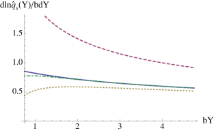
(a)

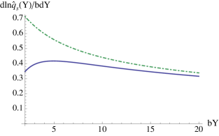
(b)

Figure 3: The logarithmic derivative of the jet quenching parameter ${\rm d}\ln\hat{q}(Y)/{\rm d}Y$ for running coupling evolution as a function of $bY$. (a) $\rho$–independent initial condition. Continuous blue: $n=7$ truncated solution for $\rho_{0}=0$. Dashed magenta, dotted gold, dotted-dashed green: asymptotic solution given in Eq. (37) with one, two, all terms kept respectively. (b) $\rho$–dependent initial condition, cf. Eq. (19) with $\rho_{0}=2.3$ and $b=4/3$. Continuous blue: $n=10$ truncated solution. Dotted-dashed green: asymptotic solution given in Eq. (37) with all terms included.

Turning to the case of a running coupling, we observe that, even though in that case we do not dispose of an explicit solution in closed form, we can still check the convergence of the truncated solution, by comparing successive truncations with the each other. We have performed such numerical tests and found that the estimate Eq. (42) for the number of terms to be kept in the series for a given value of $Y$, that is, $n\sim 2\sqrt{bY}$, is indeed reliable. Once again, the asymptotic behavior is reached already for relatively small values of the corresponding evolution time $bY$. This is illustrated in Fig. 3.a where we show the logarithmic derivative of the truncated solution for running coupling. We find that $n=6$ terms are enough to accurately reproduce the solution up to values of $bY$ close to 5, as adding more terms does not change the result. Furthermore, we see that the asymptotic solution in Eq. (37) remains quite good down to $bY\sim 1$.

As discussed earlier, in the running coupling case one eventually needs to include a non–zero value for the variable $\rho_{0}$ (cf. Eqs. (11) and Eq. (19)), otherwise the evolution becomes extremely fast since sensitive to unphysically large values of the coupling. At this level, it becomes appropriate to open a parenthesis and discuss some physical choices for the quantities $\rho_{0}$ and $Y$. As a rough estimate for the case of hot QCD matter (a weakly coupled QGP), let us use $\lambda=1/T$ with $T=500$ MeV and $L=3\div 8$ fm; this yields $Y=\ln(LT)\simeq 2\div 3$. Also, to obtain an estimate for $\rho_{0}=\ln\big{(}\hat{q}^{(0)}\lambda/\Lambda^{2}\big{)}$, we also need the tree–level jet quenching parameter. Taking (once again, as a very rough estimate) $\hat{q}^{(0)}=1\ {\rm GeV}^{2}/$fm together with $\Lambda=200$ MeV, one finds $\rho_{0}\simeq\ln 10\simeq 2.3$. Closing the parenthesis and returning to Fig. 3.b, we notice that, by including a non–zero value $\rho_{0}=2.3$ in the calculation, one does not alter the asymptotic behavior of $\ln\hat{q}_{s}(Y)$, as shown in Eq. (37) (albeit the approach towards asymptotics appears to be slightly slower than for $\rho_{0}=0$, cf. Fig. 3.a).

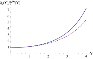
(a)

(b)

Figure 4: Enhancement factor for the jet quenching parameter $\hat{q}$ as a function of $Y$. (a) Fixed coupling evolution with $\bar{\alpha}_{s}=0.33$. Continuous blue: $\rho$–independent initial condition. Dashed magenta: initial condition proportional to $\rho+\rho_{0}$ with $\rho_{0}=2.3$ and $\rho=Y$. (b) Running coupling evolution with $b=4/3$ and $\rho_{0}=2.3$. Continuous blue: $\rho$–independent initial condition. Dashed magenta: initial condition proportional to $\ln(\rho+\rho_{0})/(\rho+\rho_{0})$ with $\rho_{0}=2.3$ and $\rho=Y$. At $Y=3$ and for constant initial condition the enhancement factor is 3.4 for both types of evolution. For the $\rho$–dependent initial condition the corresponding factor is 2.9 for fixed coupling and 3.6 for running coupling.

Finally, in Fig. 4 we show the enhancement factor $\hat{q}_{s}(Y)/\hat{q}^{(0)}(Y)$ for both fixed and running coupling and for two different types of initial conditions. (The function $\hat{q}^{(0)}(Y)$ is the respective initial condition in Eq. (19) evaluated at $\rho=Y$.) As visible in these figures, there is roughly an enhancement factor $3\div 4$ in the value of the jet quenching parameter after after a quantum evolution of three units in rapidity, for both fixed and running coupling. (To estimate the uncertainty coming from the choice of the shift $\rho_{0}$, we vary the latter in between 1.8 and 2.8. We thus find that, in the RC case, the enhancement factor varies from 3.9 to 3.0, whereas with FC, it is almost constant and approximately equal to 2.9.) The fact that this factor appears to be similar with both fixed and running coupling is likely to be ‘accidental’, in the sense that the respective predictions will start deviating from each other for larger values of $Y$. To render this manifest, we compare on a same plot, in Fig. 5, the enhancements factors corresponding to both fixed and running coupling (with constant initial conditions, for simplicity), for values of $Y$ which are only slightly larger than those in Fig. 4. Whereas the two curves closely overlap up to $Y=3$ (in agreement with Fig. 4), they differ by a factor of 2 when $Y=5$. With further increasing $Y$, this deviation is rapidly growing.

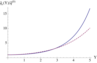
Figure 5: Enhancement factor for the jet quenching parameter $\hat{q}$ as a function of $Y$, for both fixed and running coupling and with $\rho$–independent initial conditions. Continuous blue: fixed coupling evolution with $\bar{\alpha}_{s}=0.33$. Dashed magenta: running coupling evolution with $b=4/3$ and $\rho_{0}=2.3$.

- (1) R. Baier, Y. L. Dokshitzer, A. H. Mueller, S. Peigne, and D. Schiff, “Radiative Energy Loss of High Energy Quarks and Gluons in a Finite-Volume Quark-Gluon Plasma,” Nucl. Phys. B483 (1997) 291–320, arXiv:hep-ph/9607355.
- (2) R. Baier, Y. L. Dokshitzer, A. H. Mueller, S. Peigne, and D. Schiff, “Radiative Energy Loss and P(T)-Broadening of High Energy Partons in Nuclei,” Nucl. Phys. B484 (1997) 265–282, arXiv:hep-ph/9608322.
- (3) B. G. Zakharov, “Fully Quantum Treatment of the Landau-Pomeranchuk-Migdal Effect in QED and QCD,” JETP Lett. 63 (1996) 952–957, arXiv:hep-ph/9607440.
- (4) B. G. Zakharov, “Radiative Energy Loss of High Energy Quarks in Finite-Size Nuclear Matter and Quark-Gluon Plasma,” JETP Lett. 65 (1997) 615–620, arXiv:hep-ph/9704255.
- (5) R. Baier, Y. L. Dokshitzer, A. H. Mueller, and D. Schiff, “Medium-Induced Radiative Energy Loss: Equivalence Between the Bdmps and Zakharov Formalisms,” Nucl. Phys. B531 (1998) 403–425, arXiv:hep-ph/9804212.
- (6) U. A. Wiedemann, “Gluon Radiation Off Hard Quarks in a Nuclear Environment: Opacity Expansion,” Nucl. Phys. B588 (2000) 303–344, arXiv:hep-ph/0005129.
- (7) U. A. Wiedemann, “Jet Quenching Versus Jet Enhancement: a Quantitative Study of the Bdmps-Z Gluon Radiation Spectrum,” Nucl. Phys. A690 (2001) 731–751, arXiv:hep-ph/0008241.
- (8) P. B. Arnold, G. D. Moore, and L. G. Yaffe, “Photon Emission from Quark Gluon Plasma: Complete Leading Order Results,” JHEP 12 (2001) 009, arXiv:hep-ph/0111107.
- (9) P. B. Arnold, G. D. Moore, and L. G. Yaffe, “Photon and Gluon Emission in Relativistic Plasmas,” JHEP 06 (2002) 030, arXiv:hep-ph/0204343.
- (10) Y. Mehtar-Tani, C. A. Salgado, and K. Tywoniuk, “Antiangular Ordering of Gluon Radiation in QCD Media,” Phys. Rev. Lett. 106 (2011) 122002, arXiv:1009.2965 [hep-ph].
- (11) Y. Mehtar-Tani, C. A. Salgado, and K. Tywoniuk, “Jets in QCD Media: from Color Coherence to Decoherence,” Phys. Lett. B707 (2012) 156–159, arXiv:1102.4317 [hep-ph].
- (12) J. Casalderrey-Solana and E. Iancu, “Interference Effects in Medium-Induced Gluon Radiation,” JHEP 08 (2011) 015, arXiv:1105.1760 [hep-ph].
- (13) J.-P. Blaizot, F. Dominguez, E. Iancu, and Y. Mehtar-Tani, “Medium-induced gluon branching,” JHEP 1301 (2013) 143, arXiv:1209.4585 [hep-ph].
- (14) J.-P. Blaizot, E. Iancu, and Y. Mehtar-Tani, “Medium-induced QCD cascade: democratic branching and wave turbulence,” Phys.Rev.Lett. 111 (2013) 052001, arXiv:1301.6102 [hep-ph].
- (15) J.-P. Blaizot, F. Dominguez, E. Iancu, and Y. Mehtar-Tani, “Probabilistic picture for medium-induced jet evolution,” arXiv:1311.5823 [hep-ph].
- (16) T. Liou, A. Mueller, and B. Wu, “Radiative -broadening of high-energy quarks and gluons in QCD matter,” Nucl.Phys. A916 (2013) 102–125, arXiv:1304.7677 [hep-ph].
- (17) E. Iancu, “The non-linear evolution of jet quenching,” arXiv:1403.1996 [hep-ph].
- (18) J.-P. Blaizot and Y. Mehtar-Tani, “Renormalization of the jet-quenching parameter,” arXiv:1403.2323 [hep-ph].
- (19) A. De Rujula, S. Glashow, H. D. Politzer, S. Treiman, F. Wilczek, and A. Zee, “Possible NonRegge Behavior of Electroproduction Structure Functions,” Phys.Rev. D10 (1974) 1649.
- (20) V. Gribov and L. Lipatov, “Deep inelastic e p scattering in perturbation theory,” Sov.J.Nucl.Phys. 15 (1972) 438–450.
- (21) Y. L. Dokshitzer, “Calculation of the Structure Functions for Deep Inelastic Scattering and e+ e- Annihilation by Perturbation Theory in Quantum Chromodynamics.,” Sov.Phys.JETP 46 (1977) 641–653.
- (22) G. Altarelli and G. Parisi, “Asymptotic Freedom in Parton Language,” Nucl.Phys. B126 (1977) 298.
- (23) L. Lipatov, “Reggeization of the Vector Meson and the Vacuum Singularity in Nonabelian Gauge Theories,” Sov.J.Nucl.Phys. 23 (1976) 338–345.
- (24) E. Kuraev, L. Lipatov, and V. S. Fadin, “The Pomeranchuk Singularity in Nonabelian Gauge Theories,” Sov.Phys.JETP 45 (1977) 199–204.
- (25) I. Balitsky and L. Lipatov, “The Pomeranchuk Singularity in Quantum Chromodynamics,” Sov.J.Nucl.Phys. 28 (1978) 822–829.
- (26) I. Balitsky, “Operator expansion for high-energy scattering,” Nucl. Phys. B463 (1996) 99–160, arXiv:hep-ph/9509348.
- (27) Y. V. Kovchegov, “Small-x F2 structure function of a nucleus including multiple pomeron exchanges,” Phys. Rev. D60 (1999) 034008, arXiv:hep-ph/9901281.
- (28) J. Jalilian-Marian, A. Kovner, A. Leonidov, and H. Weigert, “The BFKL equation from the Wilson renormalization group,” Nucl. Phys. B504 (1997) 415–431, arXiv:hep-ph/9701284.
- (29) J. Jalilian-Marian, A. Kovner, and H. Weigert, “The Wilson renormalization group for low x physics: Gluon evolution at finite parton density,” Phys. Rev. D59 (1999) 014015, arXiv:hep-ph/9709432.
- (30) A. Kovner, J. G. Milhano, and H. Weigert, “Relating different approaches to nonlinear QCD evolution at finite gluon density,” Phys. Rev. D62 (2000) 114005, arXiv:hep-ph/0004014.
- (31) H. Weigert, “Unitarity at small Bjorken x,” Nucl. Phys. A703 (2002) 823–860, arXiv:hep-ph/0004044.
- (32) E. Iancu, A. Leonidov, and L. D. McLerran, “Nonlinear gluon evolution in the color glass condensate. I,” Nucl. Phys. A692 (2001) 583–645, arXiv:hep-ph/0011241.
- (33) E. Iancu, A. Leonidov, and L. D. McLerran, “The renormalization group equation for the color glass condensate,” Phys. Lett. B510 (2001) 133–144, arXiv:hep-ph/0102009.
- (34) E. Ferreiro, E. Iancu, A. Leonidov, and L. McLerran, “Nonlinear gluon evolution in the color glass condensate. II,” Nucl. Phys. A703 (2002) 489–538, arXiv:hep-ph/0109115.
- (35) F. Gelis, E. Iancu, J. Jalilian-Marian, and R. Venugopalan, “The Color Glass Condensate,” Ann.Rev.Nucl.Part.Sci. 60 (2010) 463–489, arXiv:1002.0333 [hep-ph].
- (36) Y. V. Kovchegov and E. Levin, Quantum chromodynamics at high energy. Cambridge University Press, 2012.
- (37) E. Iancu, K. Itakura, and L. McLerran, “Geometric scaling above the saturation scale,” Nucl. Phys. A708 (2002) 327–352, arXiv:hep-ph/0203137.
- (38) A. Mueller and D. Triantafyllopoulos, “The Energy dependence of the saturation momentum,” Nucl.Phys. B640 (2002) 331–350, arXiv:hep-ph/0205167 [hep-ph].
- (39) S. Munier and R. B. Peschanski, “Traveling wave fronts and the transition to saturation,” Phys.Rev. D69 (2004) 034008, arXiv:hep-ph/0310357 [hep-ph].
- (40) P. B. Arnold, “Simple Formula for High-Energy Gluon Bremsstrahlung in a Finite, Expanding Medium,” Phys. Rev. D79 (2009) 065025, arXiv:0808.2767 [hep-ph].
- (41) P. B. Arnold and W. Xiao, “High-energy jet quenching in weakly-coupled quark-gluon plasmas,” Phys.Rev. D78 (2008) 125008, arXiv:0810.1026 [hep-ph].
- (42) S. Caron-Huot, “O(g) plasma effects in jet quenching,” Phys.Rev. D79 (2009) 065039, arXiv:0811.1603 [hep-ph].
- (43) D. Triantafyllopoulos, “The Energy dependence of the saturation momentum from RG improved BFKL evolution,” Nucl.Phys. B648 (2003) 293–316, arXiv:hep-ph/0209121 [hep-ph].
- (44) B. Wu, “On –broadening of high energy partons associated with the LPM effect in a finite-volume QCD medium,” JHEP 1110 (2011) 029, arXiv:1102.0388 [hep-ph].
- (45) L. D. McLerran and R. Venugopalan, “Computing quark and gluon distribution functions for very large nuclei,” Phys. Rev. D49 (1994) 2233–2241, arXiv:hep-ph/9309289.
- (46) L. D. McLerran and R. Venugopalan, “Green’s functions in the color field of a large nucleus,” Phys. Rev. D50 (1994) 2225–2233, arXiv:hep-ph/9402335.
- (47) G. Beuf, “Universal behavior of the gluon saturation scale at high energy including full NLL BFKL effects,” arXiv:1008.0498 [hep-ph].
- (48) A. H. Mueller and H. Navelet, “An Inclusive Minijet Cross-Section and the Bare Pomeron in QCD,” Nucl. Phys. B282 (1987) 727.
- (49) D. Binosi and L. Theussl, “JaxoDraw: A Graphical user interface for drawing Feynman diagrams,” Comput.Phys.Commun. 161 (2004) 76–86, arXiv:hep-ph/0309015 [hep-ph].