Adaptive timestep control for nonstationary solutions of the Euler equations

Abstract

In this paper we continue our work on adaptive timestep control for weakly nonstationary problems [37]. The core of the method is a space-time splitting of adjoint error representations for target functionals due to Süli [39] and Hartmann [21]. The main new ingredients are (i) the extension from scalar, 1D, conservation laws to the 2D Euler equations of gas dynamics, (ii) the derivation of boundary conditions for a new formulation of the adjoint problem and (iii) the coupling of the adaptive time-stepping with spatial adaptation. For the spatial adaptation, we use a multi resolution-based strategy developed by Müller [28], and we combine this with an implicit time discretization. The combined space-time adaptive method provides an efficient choice of timesteps for implicit computations of weakly nonstationary flows. The timestep will be very large in time intervalls of stationary flow, and becomes small when a perturbation enters the flow field. The efficiency of the solver is investigated by means of an unsteady inviscid 2D flow over a bump.

1 Introduction

Today, there is broad consensus that the numerical solution of compressible flow equations requires a highly resolved mesh to simulate accurately the different scales of the flow field and its boundaries. Adaptive grid methods can significantly improve the efficiency by concentrating cells only where they are most required, thus reducing storage requirements as well as the computational time. There has been a tremendous amount of research designing, analyzing and implementing codes which are adaptive in space, see, e.g., [8, 28, 25, 30] and references therein.

Here our interest is in timestep adaptation. For stationary problems, local timesteps which are linked to the spatial gridsize are commonplace, and they are heavily built upon the fact that time-accuracy, or time synchronization is not needed. On the other hand, for fully nonstationary flows, explicit algorithms whose timestep is governed by the $C\!F\!L$ restriction of at most unity are the method of choice. In [37], we began to explore one of the remaining gaps, namely weakly nonstationary flows on which we will focus in the following. Many real world applications, like transonic flight, are perturbations of stationary flows. While time accuracy is still needed to study phenomena like aero-elastic interactions, large timesteps may be possible when the perturbations have passed. For explicit calculations of nonstationary solutions to hyperbolic conservation laws, the timestep is dictated by the $C\!F\!L$ condition due to Courant, Friedrichs and Lewy [11], which requires that the numerical speed of propagation should be at least as large as the physical one. For implicit schemes, the $C\!F\!L$ condition does not provide a restriction, since the numerical speed of propagation is infinite. Depending on the equations and the scheme, restrictions may come in via the stiffness of the resulting nonlinear problem. These restrictions are usually not as strict as in the explicit case, where the $C\!F\!L$ number should be below unity. For implicit calculations, $C\!F\!L$ numbers of much larger than 1 may well be possible. Therefore, it is a serious question how large the timestep, i.e., the $C\!F\!L$ number, should be chosen.

A possible strategy has been investigated by Ferm and Lötstedt [17] based on timestep control strategies for ODEs. Here a Runge-Kutta-Fehlberg method is applied to the semi-discretized flow equations by which the local spatial and temporal errors are estimated. These errors determine the local stepsize in time and space. Later on, this idea was also embedded in fully adaptive multiresolution finite volume schemes, see [15, 14]. Alternatively Kröner and Ohlberger [25, 30] based their space-time adaptivity upon Kuznetsov-type a posteriori $L^{1}$ error-estimates for scalar conservation laws.

In this paper we will use a space-time-split adjoint error representation to control the timestep adaptation. For this purpose, let us briefly summarize the space-time splitting of the adjoint error representation, see [16, 2, 3, 39, 21] for details. The error representation expresses the error in a target functional as a scalar product of the finite element residual with the dual solution. This error representation is decomposed into separate spatial and temporal components. The spatial part will decrease under refinement of the spatial grid, and the temporal part under refinement of the timestep. Technically, this decomposition is achieved by inserting an additional projection. Usually, in the error representation, one subtracts from the dual solution its projection onto space-time polynomials. Now, we also insert the projection of the dual solution onto polynomials in time having values which are $H^{1}$ functions with respect to space.

This splitting can be used to develop a strategy for an adaptive choice of timesteps $\Delta t_{m}$. For simplicity, we work with timesteps $\Delta t_{m}$ which are uniform in space at each time $t^{m}$, so time adaptation only means that in general, $\Delta t_{m}\neq\Delta t^{{m}+1}$. However, note that the adaptive indicator developed here would permit us to implement adaptive timesteps which are also local in space. See [4, 12, 29] for more information on local timesteps.

In contrast to the results reported in [39, 21] for scalar conservation laws we now investigate weakly nonstationary solution to the 2D Euler equations. The timestep will be very large in time intervalls of stationary flow, and becomes small when a perturbation enters the flow field.

Besides applying well-established adjoint techniques to a new test problem, we further develop a new technique (first proposed by the authors in [37]) which simplifies and accelerates the computation of the dual problem. Due to Galerkin orthogonality, the dual solution $\varphi$ does not enter the error representation as such. Instead, the relevant term is the difference between the dual solution and its projection to the finite element space, $\varphi-\varphi_{h}$. In [37] we showed that it is therefore sufficient to compute the spatial gradient of the dual solution, $w=\nabla\varphi$. This gradient satisfies a conservation law instead of a transport equation, and it can therefore be computed with the same conservative algorithm as the forward problem [37]. The great advantage is that the conservative backward algorithm can handle possible discontinuities in the coefficients robustly.

A key step is to formulate boundary conditions for the gradient $w=\nabla\varphi$ instead of $v$. Generally the boundary conditions for the dual problem come from the weighting functions of the target functional, e.g., lift or drag. To formulate boundary conditions for $w$ which are compatible with the target functional, one has to lift the well-established techniques of characteristic decompositions from the dual solution to its gradient. We will present details on that in Section 5.

We start with a very coarse, but adaptive spatial mesh. In time we first compute local timesteps according to a given $C\!F\!L$ number below unity. Then, for simplicity, we use a global timestep which is the minimum over these local timesteps. Using our error indicator, we establish timesteps which are well adapted to the physical problem at hand. The scheme detects stationary time intervals, where it switches to very high $C\!F\!L$ numbers, but reduces the timesteps appropriately as soon as a perturbation enters the flow field.

We combine our time-adaptation with the spatial adaptive multiresolution technique [28]. In the early 90’s Harten [20] proposed to use multiresolution techniques in the context of finite volume schemes applied to hyperbolic conservation laws. He employed these techniques to transform the arrays of cell averages associated with any given finite volume discretization into a different format that reveals insight into the local behavior of the solution. The cell averages on a given highest level of resolution (reference mesh) are represented as cell averages on some coarse level, where the fine scale information is encoded in arrays of detail coefficients of ascending resolution.

In Harten’s original approach, the multiresolution decomposition [20] is used to control a hybrid flux computation by which computational time for the flux computation can be saved, whereas the overall computational complexity is not reduced but still stays proportional to the number of cells on the uniformly fine reference mesh. Opposite to this strategy, threshold techniques are applied to the multiresolution decomposition in [19, 28, 10] where detail coefficients below a threshold value are discarded. By means of the remaining significant details a locally refined mesh is determined whose complexity is significantly reduced in comparison to the underlying reference mesh. We will use this approach for the local adaptation in space. These techniques have been applied successfully to the stationary and instationary Euler equations [6].

In the present work, we are interested to combine the multi resolution-based grid adaptation with adjoint techniques to solve efficiently nonstationary problems. The advantage of this space adaptive method is that it also provides an efficient break condition for the Newton iteration in the implicit time integration, see Section 6.4.

The paper is organized as follows. We start with a brief description of the fluid equations and their discretization by implicit finite volume schemes, see Section 2. The adjoint error control is presented in Section 3, followed by the space-time splitting and the error estimates in Section 4. Section 5 is about the boundary conditions of the forward problem, the dual problem and the conservative dual problem. In Section 6 we will present some details on the numerical realization: The adaptive method in time and grid generation. To improve the efficiency of the scheme we employ multiresolution techniques. In Section 6.2 we give a short review of the multi resolution decomposition, upon which the adaptation in space is based. In Section 7 we present the nonstationary test case, a 2D Euler transonic flow around a circular arc bump in a channel. In Sections 8 and 9 results of the fully implicit and a mixed explicit-implicit time adaptive strategy are presented to illustrate the efficiency of the scheme. In Section 10 we summarize our results.

2 Governing equations and finite volume scheme

For the numerical simulation of nonstationary inviscid compressible fluids we solve the time-dependent Euler equations in $\mathbb{R}^{d}\times\mathbb{R}_{+}^{0}$. These lead to a system of conservation equations

$$U_{t}+\nabla\cdot f(U)=0\quad\textnormal{in }\Omega_{T},$$ (1)

$$P_{-}(U^{+})\,({\mathbf{f}_{\nu}}(U^{+})-g)=0\quad\textnormal{on }\Gamma_{T}.$$ (2)

Here ${\Omega}\subset\mathbb{R}^{d}$ is the spatial domain with boundary $\Gamma\!:=\!\partial{\Omega}\subset\mathbb{R}^{d}$ and $\Omega_{T}=\Omega\times[0,T)\subset\mathbb{R}^{d}\times\mathbb{R}_{+}^{0}$ is the space-time domain with boundary $\Gamma_{T}\!:=\!\partial{\Omega_{T}}\subset\mathbb{R}^{d}\times\mathbb{R}_{+}^{0}$. ${U}=(\varrho,\varrho\,{v},\varrho\,E)^{\mathrm{T}}$ is the vector of conservative variables (density of mass, momentum, specific total energy) and ${f}=(\varrho\,{v},\varrho\,vv^{\mathrm{T}}+pI,v\,(\varrho\,E+p))^{\mathrm{T}}=(f_{1},\dots,f_{d{{\color[rgb]{0,0,1}}}{{\color[rgb]{0,0,0}+2}}})^{\mathrm{T}}$ the array of the corresponding convective fluxes $f_{i}$, $i=1,\dots,d{{\color[rgb]{0,0,1}}}{{\color[rgb]{0,0,0}+2}}$, in the $i$th coordinate direction. $p$ is the pressure and ${v}$ the fluid velocity. The system of equations is closed by the perfect gas equation of state $p=\varrho\,(E-0.5\,{v}^{2})(\gamma-1)$ with $\gamma=1.4$ (air).

We denote by $\mathbf{f}(U):=(f(U),U)$ the space-time flux, by $\nu$ the space-time outward normal to $\Omega_{T}$, and by ${\mathbf{f}_{\nu}}(U):=\mathbf{f}(U)\cdot\nu$ the space-time normal flux. $U^{+}$ is the interior trace of $U$ at the boundary ${\Gamma_{T}}$ (or any other interface used later on). Given the boundary value $U^{+}$ and the corresponding Jacobian matrix ${\mathbf{f}_{\nu}}^{\prime}(U^{+})$, let $P_{-}(U^{+})$ be the $(d+2)\times(d+2)$-matrix which realizes the projection onto the eigenspace of ${\mathbf{f}_{\nu}}^{\prime}(U^{+})$ corresponding to negative eigenvalues (see Section 5). Then the matrix-vector product $P_{-}(U^{+})\,{\mathbf{f}_{\nu}}(U^{+})$ is the incoming component of the normal flux at the boundary, and it is prescribed in (2). Accordingly we define $P_{+}(U^{+})$, with respect to the positive eigenvalues. See Section 5 for details.

Since it is well-known that solutions $U$ will develop singularities in finite time [31, 27, 36], we pass to the weak formulation of (1), (2). It is not fully understood to which space the weak solution should belong, but loosely based upon the recent work [13] we assume that the solution space is

$$\mathcal{U}:=\textnormal{BV}({\Omega_{T}}).$$

This implies that $U,f(U)\in L^{1}_{\textnormal{loc}}({\Omega_{T}})$ and that $d$-dimensional traces exist. As the space of test functions we choose

$$\mathcal{V}:=\{\varphi\in W^{1,\infty}({\Omega_{T}})\,|\,\text{supp}\,\varphi\subset\subset{\overline{\Omega_{T}}}\},$$

which is consistent with the regularity theory in [41]. Note that the test functions may take non-zero boundary values. We call $U\in\mathcal{U}$ a weak solution of (1), (2) if for all $\varphi\in\mathcal{V}$

$$\int_{\Omega_{T}}(U\varphi_{t}+f(U)\nabla\varphi)\,dV(x,t)-\int_{{\Gamma_{T}}}P_{+}(U^{+})\,{\mathbf{f}_{\nu}}(U^{+})\varphi\,dS(x,t)$$

$$\;\;\;\;=\;\int_{{\Gamma_{T}}}P_{-}(U^{+})\,g\varphi\,dS(x,t).$$ (3)

We approximate (3) by a first or second order finite volume scheme with implicit Euler time discretization. The computational spatial grid ${\Omega_{h}}$ is a set of open cells $V_{i}$ such that

$$\bigcup_{i}\;\overline{V_{i}}={\overline{\Omega}}.$$

The intersection of the closures of two different cells is either empty or a union of common faces and vertices. Furthermore let ${\mathcal{N}}(i)$ be the set of cells that have a common face with the cell $i$, $\partial V_{i}$ the boundary of the cell $V_{i}$ and for $j\in{\mathcal{N}}(i)$ let $\Gamma_{ij}:=\partial V_{i}\cap\partial V_{j}$ be the interface between the cells $i$ and $j$ and $n_{ij}$ the outer spatial normal to $\Gamma_{ij}$ corresponding to cell $i$. Since we will work on curvilinear grids, we require that the geometric consistency condition

$$\sum_{j\in N(i)}|\Gamma_{ij}|n_{ij}=0$$ (4)

holds for all cells.

Let us define a partition of our time interval $I:=(0,T)$ into subintervals ${I_{m}}=[t_{m-1},t_{m}]$, $1\leq{m}\leq N$, where

$$0=t_{0}<t_{1}<\ldots<t_{m}<\ldots<t_{N}=T.$$

The timestep size is denoted by $\Delta t_{m}:=t_{m}-t_{m-1}$. Later on this partition will be defined automatically by the adaptive algorithm. We also denote the space-time cells and faces by ${V_{i}^{m}}:={V_{i}}\times{I_{m}}$ and ${\Gamma_{ij}^{m}}:={\Gamma_{ij}}\times{I_{m}}$, respectively. Given this space-time grid the implicit finite volume discretization of (3) can be written as

$$U_{i}^{m}+\frac{\Delta t_{m}}{|V_{i}|}\,\sum_{j\in{\mathcal{N}}(i)}|\Gamma_{ij}|\,F_{ij}^{m}=U_{i}^{m-1}\;\;\;\text{for}\;\;{m}\geq 1.$$ (5)

It computes the approximate cell averages $U^{m}_{i}$ of the conserved variables on the new time level. For interior faces ${\Gamma_{ij}}$, the canonical choice for the numerical flux is a Riemann solver,

$$F_{ij}^{m}:=F_{\textnormal{riem}}(U_{i}^{m},U_{j}^{m},n_{ij})$$ (6)

consistent with the normal flux $f_{n}(U)=f(U)\cdot n_{ij}$. In the numerical experiments in Sections 8 and 9 we choose Roe’s solver [34]. If ${\Gamma_{ij}}\subset\partial{\Omega_{T}}=:{\Gamma_{T}}$, then we follow the definition (3) of a weak solution and define the numerical flux at the boundary by

$$F_{ij}^{m}:=P_{+}(U_{i}^{m})\,\mathbf{f}_{\nu_{ij}}(U_{i}^{m})+P_{-}(U_{i}^{m})\,g_{ij}^{m},$$ (7)

where $g_{ij}^{m}$ is the average of $g$ over ${\Gamma_{ij}^{m}}$.

For simplicity of presentation we neglect in our notation that due to higher order reconstruction the numerical flux usually depends on an enlarged stencil of cell averages.

3 Adjoint error control - adaptation in time

In order to adapt the timestep sizes we use a method which involves adjoint error techniques. We have applied this approach successfully to Burgers’ equation in [37]. Now we present an extension of this approach to systems of conservation laws.

Since a finite volume discretization in space and a backward Euler step in time are a special case of a Discontinuous Galerkin discretization, techniques based on a variational formulation can be transferred to finite volume methods.

The key tool for the time adaptive method is a space-time splitting of adjoint error representations for target functionals due to Süli [39] and Hartmann [21]. It provides an efficient choice of timesteps for implicit computations of weakly nonstationary flows. The timestep will be very large in time intervalls of stationary flow, and become small when a perturbation enters the flow field.

3.1 Variational Formulation

In this section we rewrite the finite volume method as a Galerkin method, which makes it easier to apply the adjoint error control techniques.

Let us first introduce the space-time numerical fluxes. Let ${V_{i}^{m}}=V_{i}\times{I_{m}}\in{\Omega_{T,h}}$ be a space-time cell, and let $\gamma\subset\partial{V_{i}^{m}}$ be one of its faces, with outward unit normal $\nu$. There are two cases: if $\nu$ points into the spatial direction, then $\gamma={\Gamma_{ij}}\times{I_{m}}$ and $\nu=(n,0)$. If it points into the positive time direction, then $\gamma=V_{i}\times\{t_{m}\}$, and $\nu=(0,1)$. Now we define the space-time flux by

$${\mathcal{F}_{\nu}^{m}}(U_{h})=\left\{\begin{array}[]{cl}F_{ij}^{m}\;\;\text{from}\;\;\eqref{eq.euler_fv_fint}&~{}~{}\text{if}~{}~{}\nu={n_{ij}}\;\;\text{and}~{}~{}\gamma\in{\mathcal{E}_{T,h}^{\textnormal{int}}}\\ F_{ij}^{m}\;\;\text{from}\;\;\eqref{eq.euler_fv_fext}&~{}~{}\text{if}~{}~{}\nu={n_{ij}}\;\;\text{and}~{}~{}\gamma\in{\mathcal{E}_{T,h}^{\textnormal{ext}}}\\ (1-\theta)U_{i}^{m-1}+\theta U_{i}^{m}&~{}~{}\text{if}~{}~{}\nu=(0,1)\;\;\text{and}~{}~{}{m}\geq 1\\ U_{i}^{0}&~{}~{}\text{if}~{}~{}\nu=(0,1)\;\;\text{and}~{}~{}{m}=0\end{array}\right.$$ (12)

where ${\mathcal{E}_{T,h}^{\textnormal{int}}}$ are the interior faces and ${\mathcal{E}_{T,h}^{\textnormal{ext}}}$ the boundary faces. In the third case, $\theta\in[0,1]$, so the numerical flux in time direction is a convex combination of the cell averages at the beginning and the end of the timestep. Different values of $\theta$ will yield different time discretizations, e.g., explicit Euler for $\theta=0$, implicit Euler for $\theta=1$.

Let ${{\mathcal{V}}_{h}}:=W^{1,\infty}({\Omega_{T,h}})$ be the space of piecewise Lipschitz-continuous functions. Now we introduce the semi-linear form $N$ by

$$N :\;\;\;\;\;\;\mathcal{U}\times{{\mathcal{V}}_{h}}\to\mathbf{R}$$

$$N(U,\varphi) :=\sum_{i,{m}}({\mathcal{F}_{\nu}^{m}}(U),\varphi)_{{\partial V_{i}^{m}}}$$

$$\;\;-\sum_{i,{m}}\left((U,\varphi_{h,t})_{{V_{i}^{m}}}+(f(U),\nabla\varphi)_{{V_{i}^{m}}}.\right)$$ (13)

Here and below the sum is over the set $\{(i,{m})\,|\,{V_{i}^{m}}\in{\Omega_{T,h}}\}$, i.e., all gridcells. Now we rewrite the finite volume method (5) as a first order Discontinuous Galerkin method (DG0):

$$\text{Find}\;\;U_{h}\in{\mathcal{V}_{h}^{0}}\;\;\;\;\text{such that}\;\;\;\;N(U_{h},\varphi_{h})=0\quad\quad\forall\varphi_{h}\in{\mathcal{V}_{h}^{0}},$$ (14)

where ${\mathcal{V}_{h}^{0}}$ is the space of piecewise constant functions over ${\Omega_{T,h}}$.

Remark 3.1.

(i) For the DG0 method, $U_{h},\varphi\in{\mathcal{V}_{h}^{0}}$ are piecewise constant, so the last two terms in (14), containing derivatives of $\varphi$, disappear. Moreover, due to the geometric condition (4)

$$\sum\limits_{\{j\,|\,{\Gamma_{ij}^{m}}\subset{\partial V_{i}^{m}}\}}\mathbf{f}(U_{i}^{m})\cdot\nu_{ij}^{m}=0$$

holds for all cells ${V_{i}^{m}}$. Therefore, the DG0 solution may be characterized by: Find $U_{h}\in{\mathcal{V}_{h}^{0}}$ such that

$$\sum_{i,{m}}({\mathcal{F}_{\nu}^{m}}(U_{h})-{\mathbf{f}_{\nu}}(U^{+}_{h}),\varphi_{h})_{{\partial V_{i}^{m}}}=0\quad\quad\forall\varphi_{h}\in{\mathcal{V}_{h}^{0}}.$$ (15)

This form is convenient to localize our error representation later on.

(ii) The Galerkin orthogonality (15) also holds for the first and higher order finite volume schemes. These schemes satisfy (15) due to their conservation property for local cell averages, which correspond to piecewise constant test functions $\varphi_{h}$. As we go along, we will see that all the error representations developed in this paper hold for higher order finite volume schemes, as well. The reason is that we will only test with $\varphi_{h}\in{\mathcal{V}_{h}^{0}}$.

3.2 Adjoint error representation for target functionals

In this section we define the class of target functionals $J(U)$ treated in this paper, state the corresponding adjoint problem and prove the error representation which we will use later for adaptive timestep control.

Before we derive the main theorems, we would like to give a preview of an important difference between error representations for linear and nonlinear hyperbolic conservation laws. For linear conservation laws (and many other linear PDE’s), it is possible to express the error in a user specified functional,

$${\varepsilon_{J}} :=J(U)-J(U_{h}),$$ (16)

as a computable quantity $\eta$, so

$${\varepsilon_{J}} =\eta$$ (17)

(see, e.g., [2, 3, 39, 1, 22, 23, 40] and the references therein). In general, $\eta$ will be an inner product of the numerical residual with the solution of an adjoint problem. Below we will see that such a representation does not hold for nonlinear hyperbolic conservation laws. The nonlinearity will give rise to an additional error ${\varepsilon_{\Gamma}^{-}}$ on the inflow boundary, an error ${\varepsilon_{\Gamma}^{+}}$ on the outflow boundary, and a linearization error ${\varepsilon_{\Omega}}$ in the interior domain. Altogether, the error representation in Theorem 2 will be

$${\varepsilon_{J}}+{\varepsilon_{\Gamma}^{-}}+{\varepsilon_{\Gamma}^{+}}+{\varepsilon_{\Omega}} =\eta.$$ (18)

Our adaptation is based on equidistributing this $\eta$.

Typical examples for the functional $J$ are the lift or the drag of a body immersed into a fluid. To simplify matters we consider functionals of the following form:

$$J(U)=(U,\psi)_{{\Omega_{T}}}-(P_{+}(U^{+}){\mathbf{f}_{\nu}}(U^{+}),\psi_{\Gamma})_{{\Gamma_{T}}},$$ (19)

where $\psi$ and $\psi_{\Gamma}$ are weighting functions in the interior of the space-time domain $\Omega_{T}$ and at the boundary $\Gamma_{T}$. This class of functionals includes lift and drag and also the functional used in the numerical eperiments in Section 6 (see Section 5.4 for details).

Let $U_{h}$ be a solution of the first or higher order finite volume scheme (5). As pointed out in Remark 3.1, these schemes are Galerkin orthogonal when tested with piecewise constant functions. As a first step towards deriving the identity (18), we generalize the well-known error representation (see, e.g., Tadmor [41, (2.16)]) from initial value problems ($\Omega=\mathbb{R}^{d}$) to the initial boundary value problem (1)–(2). For this, let ${\bar{A}}={\bar{A}}(U,U_{h})$ be the averaged Jacobian

$${\bar{A}} :=\int\limits_{0}^{1}\textnormal{D}f(U_{h}+\tau(U-U_{h}))d\tau.$$ (20)

Note that ${\bar{A}}$ is in general discontinuous with respect to $x$, and it is conservative in the sense that

$$f(U)-f(U_{h}) ={\bar{A}}\,(U-U_{h}).$$ (21)

Let ${\bar{P}}_{\pm}$ be the corresponding projection matrices. Then

Theorem 1.

Suppose $\varphi\in\mathcal{V}$ solves the adjoint problem

$$\partial_{t}\varphi+{\bar{A}}^{\mathrm{T}}\nabla\varphi =\psi\quad\;\;\mathrm{in}\;{\Omega_{T}},$$ (22)

$$\bar{P}^{\mathrm{T}}_{+}(\varphi-\psi_{\Gamma}) =0\quad\;\;\mathrm{on}\;\Gamma_{T}$$ (23)

where $\psi$ defines the functional $J(U)$ in (19). Let ${\varepsilon_{J}}$ be defined by (16) and let

$${\varepsilon_{\Gamma}^{-}} :=-((P_{-}(U^{+})-P_{-}(U_{h}^{+}))g,\varphi)_{\Gamma_{T}}$$

$${\varepsilon_{\Gamma}^{+}} :=-(P_{+}(U^{+}){\mathbf{f}_{\nu}}(U^{+})-P_{+}(U_{h}^{+}){\mathbf{f}_{\nu}}(U_{h}^{+}),\varphi-\psi_{\Gamma})_{\Gamma_{T}}.$$

Then

$${\varepsilon_{J}}+{\varepsilon_{\Gamma}^{-}}+{\varepsilon_{\Gamma}^{+}}=\eta$$ (24)

for all $\varphi_{h}\in{\mathcal{V}}_{h}^{0}$

$$\eta :=N(U_{h},\varphi)=N(U_{h},\varphi-\varphi_{h}).$$ (25)

Here $U^{+}$ and $U_{h}^{+}$ are the traces of $U$ and $U_{h}$ at the boundary ${\Gamma_{T}}=\partial{\Omega_{T}}$. In particular, $U_{h}\equiv U_{i}^{m}$ for a boundary face ${\Gamma_{ij}^{m}}$.

Remark 3.2.

For the initial line $\Omega\times\{t=0\}\subset{\Gamma_{T}}$, the projections become trivial,

$$P_{-}(U)=P_{-}(U_{h})=I,\quad P_{+}(U)=P_{+}(U_{h})=0,$$

so

$${\varepsilon_{\Gamma}^{-}}={\varepsilon_{\Gamma}^{+}}=0.$$

Similarly the boundary errors vanish at time $t=T$ and for supersonic spatial boundaries. For subsonic spatial parts of the boundary, the boundary errors cannot be computed a posteriori. Together with the error in the functional they will be estimated by the approximate error representations (24) and (33).

For the adjoint problem (22) and (23) the role of time is reversed and hence $\bar{P}^{\mathrm{T}}_{+}$ plays the role of $P_{-}$ in (2). Here $\psi_{\Gamma}$ comes from the weighting function in the functional (19). We will present details on the boundary conditions for the dual problem in Section 5. Note that the right-hand side in (24) depends on the solution $U$ not only due to the boundary term $P_{-}(U^{+})g$, but mainly because $\varphi$ is the solution of (22).

We would like to give a short proof of Theorem 1, since there are some subtleties due to the boundary conditions (2) and (23).
Proof of Theorem 1. By definitions (16) and (19) of ${\varepsilon_{J}}$ and $J$, resp.,

$${\varepsilon_{J}} =J(U)-J(U_{h})$$

$$=(U-U_{h},\psi)_{\Omega_{T}}-(P_{+}(U^{+}){\mathbf{f}_{\nu}}(U^{+})-P_{+}(U_{h}^{+}){\mathbf{f}_{\nu}}(U_{h}^{+}),\psi_{\Gamma})_{\Gamma_{T}}.$$ (26)

Using (22), (21), the definitions (3) of a weak solution and (13) of the variational form, we obtain

$$\phantom{==}(U-U_{h},\psi)_{\Omega_{T}}$$

$$=(U-U_{h},\varphi_{t}+{\bar{A}}^{\mathrm{T}}\nabla\varphi)_{\Omega_{T}}$$

$$=(U-U_{h},\varphi_{t})_{\Omega_{T}}+({\bar{A}}(U-U_{h}),\nabla\varphi)_{\Omega_{T}}$$

$$=\left((U,\varphi_{t})_{\Omega_{T}}+(f(U),\nabla\varphi)_{\Omega_{T}}\right)-\left((U_{h},\varphi_{t})_{\Omega_{T}}+(f(U_{h}),\nabla\varphi)_{\Omega_{T}}\right)$$

$$=(P_{-}(U^{+})g+P_{+}(U^{+}){\mathbf{f}_{\nu}}(U^{+}),\varphi)_{\Gamma_{T}}$$

$$\phantom{==}+N(U_{h},\varphi)-\sum_{i,{m}}({\mathcal{F}_{\nu}^{m}}(U_{h}),\varphi)_{{\partial V_{i}^{m}}}$$ (27)

Since $\varphi$ is continuous, the fluxes across interior faces cancel each other. Using the definition (7) of the boundary fluxes, we obtain

$$\sum_{i,{m}}({\mathcal{F}_{\nu}^{m}}(U_{h}),\varphi)_{{\partial V_{i}^{m}}} =\sum_{i,{m}}({\mathcal{F}_{\nu}^{m}}(U_{h}),\varphi)_{{\partial V_{i}^{m}}\cap{\Gamma_{T}}}$$

$$=\sum_{\{(i,j,{m})\,|\,{\Gamma_{ij}^{m}}\subset{\Gamma_{T}}\}}\left(P_{-}(U_{i}^{m}){g_{ij}^{m}}+P_{+}(U_{i}^{m}){\mathbf{f}_{\nu}}(U_{i}^{m}),\varphi\right)_{\Gamma_{ij}^{m}}$$

$$=\left(P_{-}(U_{h}^{+})g+P_{+}(U_{h}^{+}){\mathbf{f}_{\nu}}(U_{h}^{+}),\varphi\right)_{\Gamma_{T}}$$ (28)

where $j$ in the second line is chosen such that ${\Gamma_{ij}^{m}}\subset{\Gamma_{T}}$. Combining (26)–(28) yields

$${\varepsilon_{J}} =N(U_{h},\varphi)-\left(P_{-}(U_{h}^{+})g+P_{+}(U_{h}^{+}){\mathbf{f}_{\nu}}(U_{h}^{+}),\varphi\right)_{\Gamma_{T}}$$

$$\phantom{=.}+\,\left(P_{-}(U^{+})g+P_{+}(U^{+}){\mathbf{f}_{\nu}}(U^{+}),\varphi\right)_{\Gamma_{T}}$$

$$\phantom{=.}-\,\left(P_{+}(U^{+}){\mathbf{f}_{\nu}}(U^{+})-P_{+}(U_{h}^{+}){\mathbf{f}_{\nu}}(U_{h}^{+}),\psi_{\Gamma}\right)_{\Gamma_{T}}$$

$$=N(U_{h},\varphi)-{\varepsilon_{\Gamma}^{-}}-{\varepsilon_{\Gamma}^{+}}$$

$$=N(U_{h},\varphi-\varphi_{h})-{\varepsilon_{\Gamma}^{-}}-{\varepsilon_{\Gamma}^{+}}.$$ (29)

In the last step we have used the definition of the DG0 scheme (14). This completes the proof. $\square$

Remark 3.3.

(i) In [41] Tadmor proves the well-posedness of the Cauchy problem for the adjoint equation (23) – (22) for scalar, convex, one-dimensional conservation laws. The key observation is that, if the forward solution $U$ has jump discontinuities, then due to the entropy condition the jump of the transport coefficient $\bar{A}^{\mathrm{T}}$ has a distinct sign. This makes it possible to follow the characteristics of the adjoint problem backwards in time.
(ii) Equivalently one can define the adjoint solution via a variational formulation, see, e.g., [1, 22, 23, 40].

Besides the unknown boundary error terms ${\varepsilon_{\Gamma}^{\pm}}$ a fundamental difficulty remains if one tries to design an adaptive algorithm based on Theorem 1: Since the exact solution $U$ is not known, we cannot compute ${\bar{A}}$. Therefore we cannot approximate the solution $\varphi$ of the adjoint problem (23)–(22) as well as the error indicator $\eta$.

The following theorem, in which we replace ${\bar{A}}$ and ${\bar{P}}_{\pm}$ by

$${\tilde{A}}:={{\color[rgb]{0,0,1}}}{{\color[rgb]{0,0,0}\textnormal{D}f(U_{h})}}\quad\text{and}\quad{\tilde{P}}_{\pm}:=P_{\pm}({\tilde{A}}),$$ (30)

overcomes this difficulty.

Theorem 2.

Suppose $\varphi\in\mathcal{V}$ solves the approximate adjoint problem

$$\partial_{t}\varphi+{\tilde{A}}^{\mathrm{T}}\nabla\varphi =\psi\quad\;\;\mathrm{in}\;{\Omega_{T}},$$ (31)

$${\tilde{P}}^{\mathrm{T}}_{+}(\varphi-\psi_{\Gamma}) =0\quad\;\;\mathrm{on}\;\Gamma_{T},$$ (32)

Let ${\varepsilon_{J}}$, ${\varepsilon_{\Gamma}^{-}}$, ${\varepsilon_{\Gamma}^{+}}$ and $\eta$ be as in Theorem 1, and let

$${\varepsilon_{\Omega}} =(f(U)-f(U_{h})-{\tilde{A}}(U-U_{h}),\nabla\varphi)_{\Omega_{T}}.$$

Then

$${\varepsilon_{J}}+{\varepsilon_{\Gamma}^{-}}+{\varepsilon_{\Gamma}^{+}}+{\varepsilon_{\Omega}}=\eta.$$ (33)

Proof.

The proof is almost the same as the one of Theorem 1, except that we have to replace ${\bar{A}}$ in the third line of (27),

$$({\bar{A}}(U-U_{h}),\nabla\varphi)_{\Omega_{T}},$$

by ${\tilde{A}}$. This yields the additional term

$$(({\bar{A}}-{\tilde{A}})(U-U_{h}),\nabla\varphi)_{\Omega_{T}}=(f(U)-f(U_{h})-{\tilde{A}}(U-U_{h}),\nabla\varphi)_{\Omega_{T}}={\varepsilon_{\Omega}}.$$

This completes the proof. $\square$
A formal Taylor series expansion suggests that ${\varepsilon_{\Omega}}$ is quadratic in the error $U-U_{h}$.

4 Space-time splitting and the error estimate

The error representation (24) is not yet suitable for time adaptivity, since it combines space and time components of the residual and of the difference $\varphi-\varphi_{h}$ of the dual solution and the test function. The main result of this section is an error estimate whose components depend either on the spatial grid size $h$ or the timestep $k$, but never on both. The key ingredient is a space-time splitting of (33) based on $L^{2}$-projections. Similar space-time projections were introduced previously in [21, 39] for the linear heat equation and linear advection. In [37] we adapted them to the nonlinear Burgers equation. The projections can be generalized directly to finite element spaces and space-time Discontinuous Galerkin methods of arbitrary order.

Let ${V_{j}^{m}}=V_{j}\times{I_{m}}$ and $P_{s,r}({V_{j}^{m}})=P_{s}(V_{j})\times P_{r}({I_{m}})$ be the space of polynomials of degree $s$ on ${V_{j}}$ and $r$ on ${I_{m}}$. Furthermore let $\hat{P}_{{I_{m}}}^{r}({V_{i}^{m}})=\{w\in L^{2}({V_{i}^{m}})|w(x,\cdot)\in P_{r}({I_{m}}),\forall x\in V_{j}\}$, and $\hat{P}_{V_{j}}^{s}({V_{i}^{m}})=\{w\in L^{2}({V_{i}^{m}})|w(\cdot,t)\in P_{s}(V_{j}),\forall t\in{I_{m}}\}$. For $r\geq 0$ define the $L^{2}$-projection $\Pi_{{I_{m}}}^{r}:L^{2}({V_{i}^{m}})\to\hat{P}_{{I_{m}}}^{r}({V_{i}^{m}})$ onto piecewise polynomials in time via

$$(U(x,\cdot)-\Pi_{{I_{m}}}^{r}U(x,\cdot),\varphi(x,\cdot))_{{I_{m}}}=0\quad\forall\varphi\in\hat{P}_{{I_{m}}}^{r}({V_{i}^{m}}),\forall x\in V_{j},$$ (34)

and for $s\geq 0$ define the $L^{2}$-projection $\Pi_{V_{j}}^{s}:L^{2}({V_{i}^{m}})\to\hat{P}_{V_{j}}^{s}({V_{i}^{m}})$ onto piecewise polynomials in space via

$$(U(\cdot,t)-\Pi_{V_{j}}^{s}U(\cdot,t),\varphi(\cdot,t))_{V_{j}}=0\quad\forall\varphi\in\hat{P}_{V_{j}}^{s}({V_{i}^{m}}),\forall t\in{I_{m}}.$$ (35)

Similarly let the $L^{2}$-projection onto space-time polynomials $\Pi_{{V_{i}^{m}}}^{s,r}:=L^{2}({V_{i}^{m}})\to P_{s,r}({V_{i}^{m}})$ be defined via

$$(U-\Pi_{{V_{i}^{m}}}^{s,r}U,\varphi)_{{V_{i}^{m}}}=0\quad\forall\varphi\in P_{s,r}({V_{i}^{m}}).$$ (36)

Note that $\Pi_{{V_{i}^{m}}}^{s,r}=\Pi_{{V_{j}}}^{s}\Pi_{{I_{m}}}^{r}=\Pi_{{I_{m}}}^{r}\Pi_{{V_{j}}}^{s}$. First we choose $\varphi_{h}$ in the error representation (33) to be $\varphi_{h}=\Pi_{h,k}^{s,r}\varphi$, i.e., $\varphi_{h}\mid_{{V_{i}^{m}}}=\Pi_{{V_{j}}}^{s}\Pi_{{I_{m}}}^{r}\varphi=\Pi_{{I_{m}}}^{r}\Pi_{{V_{j}}}^{s}\varphi$. This leads to the identity

$$\varphi-\Pi_{h,k}^{s,r}\varphi=\varphi-\Pi_{{I_{m}}}^{r}\varphi+\Pi_{{I_{m}}}^{r}\varphi-\Pi_{h,k}^{s,r}\varphi=(\textnormal{id}-\Pi_{{I_{m}}}^{r})\varphi+(\textnormal{id}-\Pi_{V_{j}}^{s})\Pi_{{I_{m}}}^{r}\varphi.$$ (37)

Now we restrict ourselves to finite volume methods. These are based on space-time cell averages, and therefore the corresponding order in the DG context would be $r=s=0$, even for higher order FV schemes. Using (37), we obtain the following splitting of the error representation (33) in Theorem 2:

$$\eta =N(U_{h},\varphi)\;=N(U_{h},\varphi-\Pi_{h,k}^{0,0}\varphi)$$

$$=N(U_{h},(\textnormal{id}-\Pi_{{I_{m}}}^{0})\varphi+(\textnormal{id}-\Pi_{V_{j}}^{0})\Pi_{{I_{m}}}^{0}\varphi)$$

$$=N(U_{h},(\textnormal{id}-\Pi_{{I_{m}}}^{0})\varphi)+N(U_{h},(\textnormal{id}-\Pi_{V_{j}}^{0})\Pi_{{I_{m}}}^{0}\varphi)$$

$$=\sum_{i,{m}}({\mathcal{F}_{\nu}^{m}}(U_{h})-{\mathbf{f}_{\nu}}(U_{h}^{+}),(\textnormal{id}-\Pi_{{I_{m}}}^{0})\varphi)_{\partial V_{i}^{m}}$$

$$\phantom{=}+\sum_{i,{m}}({\mathcal{F}_{\nu}^{m}}(U_{h})-{\mathbf{f}_{\nu}}(U_{h}^{+}),(\textnormal{id}-\Pi_{V_{j}}^{0})\Pi_{{I_{m}}}^{0}\varphi)_{\partial V_{i}^{m}}$$

$$=:\eta_{k}+\eta_{h}$$ (38)

where $\eta_{k}$ is the time-component and $\eta_{h}$ the space-component of the error representation $\eta$. To summarize, we have shown the following corollary of Theorem 2:

Corollary 3.

Under the assumptions of Theorem 2, the following error representation holds:

$${\varepsilon_{J}}+{\varepsilon_{\Gamma}^{-}}+{\varepsilon_{\Gamma}^{+}}+{\varepsilon_{\Omega}}=\eta_{k}+\eta_{h}.$$ (39)

In [37] we showed by numerical experiments that $\eta_{k}$ depends only an $k$ and that $\eta_{h}$ depends only on $h$, and that they both decrease with first order. We will use the asymptotic behavior of the error term $\eta_{k}$ to derive an adaptation strategy in time.

5 Boundary conditions, the conservative dual problem and functionals at the boundary

In this section we present details of the boundary conditions for the forward (1)–(2) and the dual problem (31)–(32). Then we will recall the conservative approach to the dual problem, which we introduced in [37] and derive boundary conditions for the gradient of the dual problem. Note, that we assume that the Jacobian matrix is diagonalizable. This assumption holds for the Euler equations.

5.1 Boundary conditions for the forward and the dual problem

First we introduce some notation and state boundary conditions for the forward problem. For simplicity of notation, we restrict ourselves to the spatial domain $\Omega$ with boundary $\Gamma$, normal $n(x)$, and normal flux $f_{n}=f\cdot n$. As in (30) let ${\tilde{A}}=f_{n}^{\prime}(U_{h})$ be the Jacobian of $f_{n}$ evaluated at the approximate solution $U_{h}$, and let ${\tilde{P}}_{\pm}$ be the projection matrices which map vectors onto the eigenspaces of ${\tilde{A}}$ corresponding to positive and negative eigenvalues, respectively. They are defined in detail in (40) below.

In order to explain the boundary conditions in (2), (7), (23), and (32), we recall the theory of boundary value problems for hyperbolic systems, see, e.g., [18, 24]. Boundary values have to be prescribed along characteristics entering the domain. Therefore the solution, or the fluxes, have to be decomposed into in- and outgoing components.

Let $L=L({\tilde{A}})$ and $R=R({\tilde{A}})$ denote the $(d+2)\times(d+2)$ matrices of the left and right eigenvectors of ${{\tilde{A}}}$, and $\Lambda=\Lambda({\tilde{A}})=\textnormal{diag}(\lambda_{1}({\tilde{A}}),\dots,\lambda_{d+2}({\tilde{A}}))$ the diagonal matrix of the eigenvalues of ${\tilde{A}}$, so

$${\tilde{A}}=R\Lambda L.$$

As usual, the positive and negative parts of ${\tilde{A}}$ are

$${{\tilde{A}}_{\pm}}=R\Lambda^{\pm}L.$$

We now introduce the notations

$${\tilde{P}}_{\pm}:=RD_{\pm}L,$$ (40)

where $D_{\pm}$ is the diagonal matrix $D_{\pm}:=\textnormal{diag}(\chi^{\pm}(\lambda_{i}))$ with

$$\chi^{\pm}(\lambda)=\max(0,\textnormal{sign}(\pm\lambda)).$$

Then we observe the identities

$${\tilde{P}}_{+}{\tilde{P}}_{-}={\tilde{P}}_{-}{\tilde{P}}_{+}=0,\quad\quad{\tilde{P}}_{\pm}^{2}={\tilde{P}}_{\pm},\quad\quad{\tilde{P}}_{\pm}{\tilde{A}}=RD_{\pm}LR\Lambda L={\tilde{A}}_{\pm}.$$

Note that ${\tilde{P}}_{\pm}$ and ${\tilde{A}}$ commute:

$${\tilde{A}}{\tilde{P}}_{\pm}=R\Lambda LRD_{\pm}L=R\Lambda D_{\pm}L=RD_{\pm}\Lambda L=RD_{\pm}LR\Lambda L={\tilde{P}}_{\pm}{{\tilde{A}}}.$$

This specifies the boundary fluxes (7) for the forward finite volume solver and (32) for the linearized adjoint problem. The boundary conditions (2) and (23) are derived analogously.

5.2 The conservative dual problem

The adjoint equation (31) is a system of linear transport equations with discontinuous coefficients. Therefore, numerical approximations may easily become unstable. Another inconvenience is that in order to obtain a meaningful error representation in (33), the approximate adjoint solution $\varphi$ should not be contained in ${\mathcal{V}_{h}^{0}}$. Therefore, $\varphi$ is often computed in the more costly space $\mathcal{V}_{h}^{1}$.

In [37] we have proposed a simple alternative which helps to avoid both difficulties. Instead of computing the dual solution $\varphi$ we will compute its gradient

$$w:=\nabla\varphi,$$

which is the solution of the conservative dual problem

$$w_{t}+\nabla\cdot({\tilde{A}}^{\mathrm{T}}w)=\nabla\psi\;\;\;\text{in}\;{\Omega_{T}}.$$ (41)

This system is in conservation form, and therefore it can be solved by any finite volume or Discontinuous Galerkin scheme. Moreover, (41) may be solved in ${\mathcal{V}_{h}^{0}}$, since a piecewise constant solution $w$ already contains crucial information on the gradient of $\varphi$.

The scalar problem treated in [37] was set up in such a way that the characteristic boundary conditions for the dual problem became trivial. In the following, we develop the boundary conditions in the more general case needed in the present paper.

Denoting the flux in (41) by $H:={\tilde{A}}^{\mathrm{T}}w$, the boundary condition (32) becomes

$${\tilde{P}}_{+}^{\mathrm{T}}\,(H-H_{\Gamma})=0\;\;\;\text{on}\;{\Gamma_{T}},$$ (42)

i.e., we prescribe the incoming component ${\tilde{P}}_{+}^{\mathrm{T}}H$. Here $H_{\Gamma}$ is a given real-valued vector function, which depends on $\psi_{\Gamma}$. However, this characteristic boundary condition needs to be interpreted carefully. Using (40) and (41) and denoting the interior trace at the flux by $H_{\textnormal{int}}$, we may introduce the boundary flux by

$$H:={\tilde{P}}_{-}^{\mathrm{T}}\,H_{\textnormal{int}}+{\tilde{P}}_{+}^{\mathrm{T}}\,H_{\Gamma}\quad\textnormal{on }{\Gamma_{T}}.$$

Note that all the projections ${\tilde{P}}_{\pm}$ used below depend on the point $(x,t)\in{\Gamma_{T}}$ via the outside normal vector $\nu(x,t)$. The value ${\tilde{P}}_{-}^{\mathrm{T}}H_{\textnormal{int}}$ may be assigned from the trace $w_{\textnormal{int}}$ at the interior of the computational domain,

$${\tilde{P}}_{-}^{\mathrm{T}}\,H_{\textnormal{int}}={\tilde{P}}_{-}^{\mathrm{T}}\,({\tilde{A}}^{\mathrm{T}}w)_{\textnormal{int}}.$$

The boundary values ${\tilde{P}}_{+}^{\mathrm{T}}\,H_{\Gamma}$ are computed using the PDE

$$\varphi_{t}=-H+\psi$$ (43)

with boundary values (32),

$${\tilde{P}}_{+}^{\mathrm{T}}\,H_{\Gamma} ={\tilde{P}}_{+}^{\mathrm{T}}\,(-\varphi_{t}+\psi)|_{\Gamma}$$

$$=-({\tilde{P}}_{+}^{\mathrm{T}}\,\psi_{\Gamma})_{t}+{\tilde{P}}_{+}^{\mathrm{T}}\,\psi$$

$$\approx-\frac{1}{\Delta t_{m}}\left({\tilde{P}}_{+}^{\mathrm{T},{m}}\,\psi_{\Gamma}^{m}-{\tilde{P}}_{+}^{\mathrm{T},{m-1}}\,\psi_{\Gamma}^{m-1}\right)+{\tilde{P}}_{+}^{\mathrm{T},{m-1}}\,\psi.$$ (44)

This completes the definition of the numerical boundary conditions for the conservative dual problem.

5.3 The time component of the error representation

Let us have another look at the time component of the error representation (38),

$$\eta_{k} =\sum_{i,{m}}({\mathcal{F}_{\nu}^{m}}(U_{h})-{\mathbf{f}_{\nu}}(U_{h}^{+}),(\textnormal{id}-\Pi_{{I_{m}}}^{0})\varphi)_{\partial{V_{i}^{m}}}.$$

To compute the leading order part of $\eta_{k}$ we assume that $\varphi\in\mathcal{V}_{h}^{1}$. In this case,

$$(\textnormal{id}-\Pi_{{I_{m}}}^{0})\varphi(x,t)=\left(t-\frac{t^{m}+t^{m-1}}{2}\right)\varphi_{t}.$$

Note that $\varphi_{t}$ is piecewise constant. Using (43) we obtain

$$\eta_{k} =\sum_{i,{m}}\left({\mathcal{F}_{\nu}^{m}}(U_{h})-{\mathbf{f}_{\nu}}(U_{h}^{+}),\left(\cdot-\frac{t^{m}+t^{m-1}}{2}\right)\,(\psi-{\tilde{A}}^{\mathrm{T}}w)\right)_{\partial{V_{i}^{m}}}.$$

Since $U_{h}$ is piecewise constant, the integrals over the time-like faces $\partial V_{i}\times{I_{m}}$ drop out, and only those over the space-like faces $V_{i}\times\{t_{m}\}$ remain, so

$$\eta_{k} =\sum_{i,{m}}\left(({\mathcal{F}_{\nu}^{m}}(U_{h})-{\mathbf{f}_{\nu}}(U_{h}^{+}),\frac{\Delta t_{m}}{2}\,(\psi-{\tilde{A}}^{\mathrm{T}}w))_{V_{i}}\right.$$

$$\phantom{..}-\left.(\mathcal{F}_{\nu}^{m-1}(U_{h})-{\mathbf{f}_{\nu}}(U_{h}^{+}),\frac{\Delta t_{m}}{2}\,(\psi-{\tilde{A}}^{\mathrm{T}}w))_{V_{i}}\right)$$

$$=\sum_{i,{m}}({\mathcal{F}_{\nu}^{m}}(U_{h})-\mathcal{F}_{\nu}^{m-1}(U_{h}),\frac{\Delta t_{m}}{2}\,(\psi-{\tilde{A}}^{\mathrm{T}}w))_{V_{i}}.$$

From the definition (12) of the flux in time direction this simplifies further, namely

$$\eta_{k} =\frac{\Delta t_{m}}{2}\,\sum_{i,{m}}\left((1-\theta)(U_{i}^{m-1}-U_{i}^{{m}-2})+\theta(U_{i}^{m}-U_{i}^{m-1}),\psi-{\tilde{A}}^{\mathrm{T}}w\right)_{V_{i}}$$ (45)

(we set $U_{i}^{-1}=U_{i}^{0}$ in the first summand). Thus our temporal error indicator is simply a weighted sum of time-differences of the approximate solution $U_{h}$, and the weights can be computed from the data $\psi$ and the solution $w$ of the conservative dual problem (41).

In our adaptive strategy, we will use the localized indicators

$$\bar{\eta}_{k}^{m}:=\frac{1}{2}\,\sum\limits_{i}\left|((1-\theta)(U_{i}^{m-1}-U_{i}^{{m}-2})+\theta(U_{i}^{m}-U_{i}^{m-1}),\psi-{\tilde{A}}^{\mathrm{T}}w)_{V_{i}}\right|.$$ (46)

In the next section we present an example for the boundary conditions for the dual problem.

5.4 Example: Functionals at the boundary

In the numerical examples in Section 8 we will consider the 2D Euler equations. Let $\Gamma_{s}$ be the solid wall, where we impose the reflecting boundary condition $v\!\cdot\!n=0$. Thus the flux in normal direction $n$ is given by

$$f_{n}=p(0,n,0)^{\mathrm{T}}.$$

The eigenvalues of ${\tilde{A}}$ are $\lambda_{1}=v\cdot n-c=-c$, $\lambda_{2}=\lambda_{3}=v\cdot n=0$ and $\lambda_{4}=v\cdot n+c=c$, and we can compute

$${\tilde{P}}_{+} =R\,\mbox{{diag}}(0,0,0,1)L,$$

$${\tilde{P}}_{-} =R\,\mbox{{diag}}(1,0,0,0)L.$$

and

$${\tilde{P}}_{+}\,f_{n}(U)=\frac{p}{2}\left(\frac{1}{c},n,\frac{c}{\gamma-1}\right).$$

As our functional we choose the space-time integral of the pressure at the solid wall,

$$J(U)=\int_{0}^{T}\int_{\Gamma_{s}}p\,dS(x)\,dt.$$

If we choose

$$\psi_{\Gamma}=2(0,n,0)^{\mathrm{T}},$$

then $J(U)$ may be rewritten in terms of characteristic projections,

$$J(U)=\int_{0}^{T}({\tilde{P}}_{+}\,f_{n}(U),\psi_{\Gamma})_{\Gamma_{s}}dt.$$

Note that the functional is in the form suggested in Section 3.2. It is a modifcation of lift and drag, which is given by

$$J_{l/d}(U)=\frac{2}{\rho_{\infty}|v_{\infty}|^{2}\bar{l}}\int_{\Gamma_{s}}p\,{n}\cdot\psi\,dS(x),$$

where $\bar{l}$ denotes a reference length, the subscript $\infty$ indicates free stream quantities, $\psi$ is given by $\psi_{d}=(\textnormal{cos}(\alpha),\textnormal{sin}(\alpha))^{\mathrm{T}}$ or $\psi_{l}=(\textnormal{-sin}(\alpha),\textnormal{cos}(\alpha))^{\mathrm{T}}$ for the drag and lift coefficient, with respect to an angle of attack $\alpha$. In the numerical experiments in Sections 6–9, we will multiply $\psi_{\Gamma}$ with an additional weighting function (see (53)).

6 Numerical realization

Before we set up our test problem (Section 7) and present numerical experiments (Sections 8 – 9), we have to specify some details on the adaptive concept, the grid generation and the numerical flux evaluation on locally refined grids with hanging nodes.

6.1 Adaptive Method in time

Now we combine the multi resolution based approach introduced in Section 6.2 and the time adaptive method derived from the space-time splitting of the error representation to get a space-time adaptive algorithm:

• solve the primal problem (3) on a coarse adaptive spatial grid using uniform global timesteps, with maximal ($C\!F\!L=0.8$),

• compute the dual problem (22) and (32) and the space-time-error representation (38). In particular, compute the localized error indicators $\bar{\eta}_{k}^{m}$ using (46).

• compute the new adaptive timestep sizes depending on the temporal part of the error representation and the $C\!F\!L$ number on the new grid, aiming at an equidistribution of the error,

• solve the primal problem using the new timestep sizes on a finer spatial grid.

The advantage is, that the first computations of the primal problems and the dual problem are done on a coarse spatial grid, and therefore have low cost. These computations provide an initial guess of the timesteps for the computation on the finer spatial grid. We will restrict the timestep size from below to $C\!F\!L=0.8$, since smaller timestep sizes only add numerical diffusion to the scheme and increase the computational cost. Note that all physical effects already have to be roughly resolved on the coarse grid in order to determine a reliable guess for the timesteps on the fine grid.

We will deal with some aspects in detail in the numerical examples in Section 8 and 9.

6.2 Multi resolution decomposition and adaptation in space

A finite volume discretization is typically working on cell averages. In order to analyze the local regularity behavior of the data we employ the concept of biorthogonal wavelets [7, 9]. This approach may be considered as a natural generalization of Harten’s discrete framework [20]. The core ingredients are a hierarchy of nested grids, biorthogonal wavelets and the multi resolution decomposition. In the following we will only summarize the basic ideas. For technical details we refer the reader to the book [28] and [6], respectively.

Step 1: Multi resolution decomposition. The fundamental idea is to present the cell averages $\hat{\mbox{\boldmath$u$}}_{L}$ representing the discretized flow field at fixed time level $t^{m}$ on a given uniform highest level of resolution $l=L$ (reference mesh) associated with a given finite volume discretization (reference scheme) as cell averages $\hat{\mbox{\boldmath$u$}}_{0}$ on some coarsest level $l=0$. Here the fine scale information is encoded in arrays of detail coefficients $\mbox{\boldmath$d$}_{l}$, $l=0,\ldots,L-1$ of ascending resolution, see Figure 2.

The multi resolution decomposition is performed on a hierarchy of nested grids ${\mathcal{G}}_{l}$ with increasing resolution $l=0,\ldots,L$ determined by dyadic grid refinement of the logical space, see Figure 2.

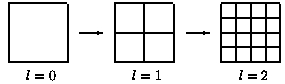
Fig. 1: Sequence of nested grids

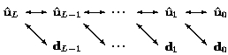
Fig. 2: multi resolution transformation

Step 2: Thresholding. It can be shown that the detail coefficients become small with increasing refinement level when the underlying function is locally smooth. This motivates us to discard all detail coefficients $d_{l,{k}}$ whose absolute values fall below a level-dependent threshold value $\varepsilon_{l}=2^{l-L}\varepsilon$ in order to compress the original data. Let ${\mathcal{D}}_{L,\varepsilon}$ be the set of significant details. The ideal strategy would be to determine the threshold value $\varepsilon$ such that the discretization error of the reference scheme, i.e., the difference between exact solution and reference scheme, and the perturbation error, i.e., the difference between the reference scheme and the adaptive scheme, are balanced, see [10].

Step 3: Prediction and grading. Since the flow field evolves in time, grid adaptation is performed after each evolution step to provide the adaptive grid at the new time level. In order to guarantee the adaptive scheme to be reliable in the sense that no significant future feature of the solution is missed, we have to predict all significant details at the new time level $n+1$ by means of the details at the old time level $n$. Let ${\tilde{\mathcal{D}}}^{m}_{L,\varepsilon}\supset{\mathcal{D}}^{m}_{L,\varepsilon}\cup{\mathcal{D}}^{m}_{L,\varepsilon}$ be the prediction set. The prediction strategy is detailed in [10]. In view of the grid adaptation step this set is additionally inflated such that it corresponds to a graded tree, i.e., the number of levels between two neighboring cells differs at most by 1.

Step 4: Grid adaptation. By means of the set ${\tilde{\mathcal{D}}}^{m}_{L,\varepsilon}$ a locally refined grid is determined. For this purpose, we recursively check (proceeding levelwise from coarse to fine) whether there exists a significant detail on a cell. If there is one, then we refine the respective cell. We finally obtain the locally refined grid with hanging nodes represented by the index set ${\mathcal{G}}_{L,\varepsilon}$, see for example Figure 9.

6.3 Grid generation.

The computational domain in our test configuration is bounded by curvilinear boundaries. For this domain we compute a parametric grid mapping ${x}:[0,1]^{2}\to\Omega$. Then a hierarchy of Cartesian grids for the parameter domain is mapped to a grid hierarchy of curvilinear meshes in the computational domain. The grid mapping is realized efficiently by a sparse B-Spline representation, cf. [6, 26]. Then the locally refined grids are determined by evaluation of this mapping. In our computations the underlying discretization is always a hierarchy of curvilinear grids.

6.4 Newton method for the nonlinear system.

The 2D Euler equations are discretized with the finite volume method on an adaptive grid. The resulting system of nonlinear equations is discretized by a Newton method in each timestep. Two delicate aspects of the Newton method are the choice of the initial value and the choice of the break condition. In our computations we choose the solution of the old timestep as initial value for the Newton iterations. The resulting system of linear equations is solved using GMRES [35] with an incomplete LU factorization (ILU) preconditioning, see [5]. The break condition for the Newton method is coupled with the threshold value of the multi resolution method: If the defect of the Newton method is below the threshold of the multi resolution representation, we will stop the iteration process.

Remark 6.1.

There are also other strategies to terminate the Newton iterations. If we assume, that in each iteration (both the nonlinear and the linear) the residuals will drop, we could choose as break condition how many times the residual has to decrease. Additionally we can set an absolute value of the number of iterations, if no other breaking condition holds. There are two main problems, which may occur. The first one is, that in the case where the solution is stationary, no iteration will decrease the error. The other problem is, that if the timestep sizes are large, and the residual is very large in the beginning and will drop down fast, the Newton iteration will stop, but will not lead to a good solution, with a small residuum. In the numerical examples we observe that the coupling with the multi resolution representation leads to very efficient results. Alternative strategies to control the timestepping could be based on the residual or the defect of the Newton-method, the boundary conditions, the $C\!F\!L$ number. For such a strategy it is obvious that we have many parameters which have to be chosen and optimized, see [32].

6.5 Computation of the dual problem

The conservative dual problem (42) is a system of $d\!\cdot\!m$ conservation laws, where $m$ is the number of equations of the forward problem and $d$ the number of space dimensions. Since for the backward solver robustness is more important than accuracy we solve (41)–(42) with a finite volume method using Lax-Friedrichs numerical flux and $C\!F\!L<1$.

7 Setup of the numerical experiment

An nonstationary variant of a classical stationary 2D Euler transonic flow, considered in [33], is investigated to illustrate the efficiency of the adaptive method.

7.1 Steady state configuration

First we consider the classical setup in the stationary case. The computational domain is a channel of $3m$ length and $2m$ height with an arc bump of $l=1m$ secant length and $h=0.024m$ height cut out, see Figure 3. At the inflow boundary, the Mach number is 0.85 and a homogeneous flow field characterized by the free-stream quantities is imposed. At the outflow boundary, characteristic boundary conditions are used. We apply slip boundary conditions across the solid walls, i.e., the normal velocity is set to zero. In the numerical examples in Section 8 the height of the channel is $2m$ and the length $6m$.

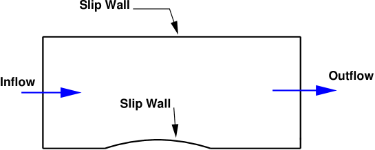
Fig. 3: Circular arc bump configuration of the computational domain $\Omega$.

Fig. 4: Adaptive grid $L=5$, to steady state solution in Figure 5 of the circular arc bump configuration.

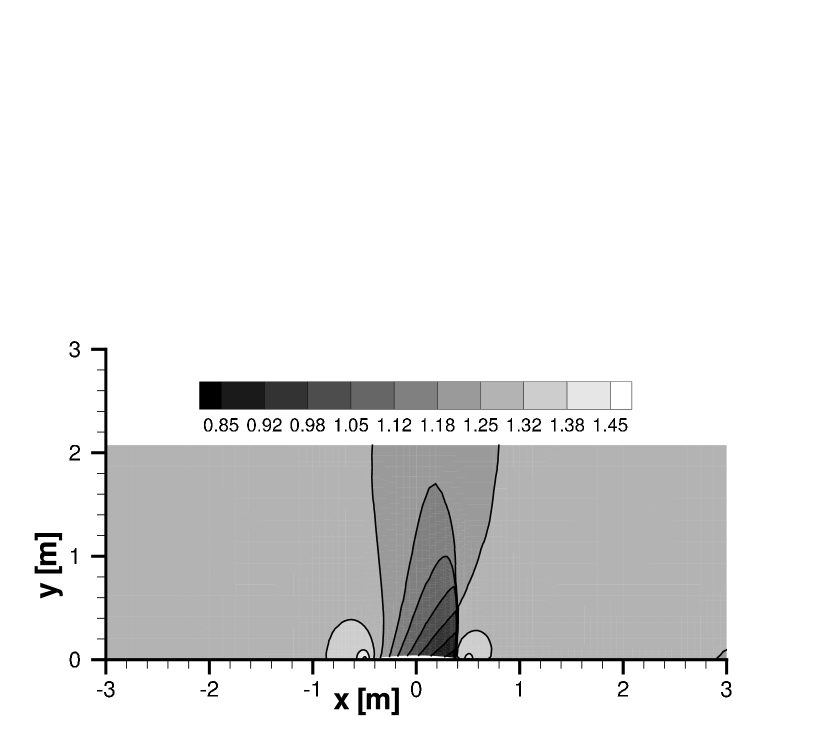
Fig. 5: Steady state solution of the circular arc bump configuration: Isolines of the density, $L=5$.

The threshold value in the grid adaptation step $\varepsilon=1\times 10^{-3}$ and computations are done on adaptive grids with finest level $L=2$ and $L=5$ respectively. In general, a smaller threshold value results in more grid refinement whereas a larger value gives locally coarser grids.

In the stationary case at Mach 0.85 there is a compression shock separating a supersonic and a subsonic domain. the stagnation areas are highly resolved, see Figures 5 and 9.

We will use this steady state solution as initial data for the nonstationary test case.

7.2 nonstationary test case

Now we define our nonstationary test case prescribing a time-dependent perturbation coming in at the inflow boundary. First we keep the boundary conditions fixed, and prescribe the corresponding stationary solution as initial data. Then we introduce, for a short time period $[t_{b},t_{e}]$, a perturbation $\alpha$ of the pressure at the left boundary, see (52). We will impose two perturbations of the inflow boundary conditions, at time $t_{b}^{1}=0.004s$ until $t_{e}^{1}=0.005s$ and at $t_{b}^{2}=0.022s$ until $t_{e}^{2}=0.023s$. These perturbations increase and decrease in a short time period of $\tau=0.00005s$. The first perturbation is about 20 percent of the pressure at the inflow boundary and the second 2 percent. The perturbations imposed move through the domain and leave it at the right boundary. Then the solution is stationary again. The total time is $t=0.029s$.

The perturbations are given by:

$$w_{p}^{i}(t)=\left\{\begin{array}[]{ccc}\left(\frac{t-t_{b}^{i}}{\tau}\right)^{2}&\mathrm{for}&t_{b}^{i}<t\leq t_{b}^{i}+\tau\\ 1&\mathrm{for}&t_{b}^{i}+\tau<t\leq t_{e}^{i}-\tau\\ \left(\frac{t-t_{e}^{i}}{\tau}\right)^{2}&\mathrm{for}&t_{e}^{i}-\tau<t\leq t_{e}^{i}\end{array}\right.,$$

$$p_{in}(t)=p_{\infty}w_{p}(t)=p_{\infty}\left\{\begin{array}[]{ccc}1&\mathrm{for}&t\leq t_{b}^{1}\\ 1+\alpha^{1}w_{p}^{1}(t)&\mathrm{for}&t_{b}^{1}<t\leq t_{e}^{1}\\ 1&\mathrm{for}&t_{e}^{1}<t\leq t_{b}^{2}\\ 1+\alpha^{2}w_{p}^{2}(t)&\mathrm{for}&t_{b}^{2}<t\leq t_{e}^{2}\\ 1&\mathrm{for}&t_{e}^{2}<t\end{array}\right.$$ (52)

with perturbation parameters listed in Table 1.

$i$	$\alpha^{i}$	$t_{b}^{i}[s]$	$t_{e}^{i}[s]$	$\tau^{i}[s]$
1	0.2	0.004	0.005	0.00005
2	0.02	0.022	0.023	0.00005

Table 1: Parameters of the perturbations $w_{p}^{i},i=1,2$ at the left boundary to equation (52).

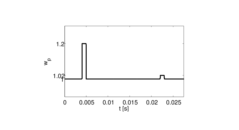
Fig. 6: Weighting function of the perturbation. $p_{in}(t)=p_{\infty}w_{p}(t)$

The first computation is done on an adaptive grid with finest level $L=2$. We also compute the dual solution and the error representation on this level. Using the time-space-split error representation (38) we derive a new timestep distribution aiming at an equidistribution of the error. Finally this is modified by imposing a $C\!F\!L$ restriction from below.

We aim to equidistribute the error and prescribe a tolerance $\;T\!ol(5)=2^{-3}\bar{\eta}_{k}^{ref}\,$, where $\bar{\eta}_{k}^{ref}$ is the temporal error from the computation on level $L=2$.

For this set-up we will show that the adaptive spatial refinement together with the time-adaptive method will lead to an efficient computation. The multi resolution method provides a well-adapted spatial representation of the solution, and the dual solution will detect time-domains where the solution is stationary. In these domains, the equidistribution strategy will choose large timesteps.

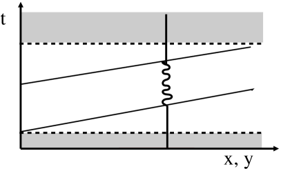
Fig. 7: Schematic illustration of the nonstationary test case. Left: perturbation at the left boundary. Right: nonstationary (white) and stationary (grey) time domains of the solution

7.3 Target functional

Now we set up the target functional. The functional $J(U)$ is chosen as a weighted average of the normal force component exerted on the bump and at the boundaries before and behind the bump:

$$J(U)=\sum_{i=1}^{7}\int_{0}^{T}\int_{\kappa_{i}}p\,\psi_{i}(x,y)ds$$ (53)

with

$$\kappa_{i} =\left\{(x,y)\in\Gamma\,:\,x\in[x_{i}-0.25,x_{i}+0.25]\right\}$$

$$\psi_{i}(x) =(x-(x_{i}-0.25))^{2}(x+(x_{i}+0.25))^{2}/0.25^{4},\quad x\in\kappa_{i}.$$

Here $\Gamma$ is only the bottom part of $\Gamma$. In all computations presented in this section the functional (53) is chosen, which is the pressure averaged at several points at the bump in front and behind the bump. The $x$-coordinates of these points at the bottom are $x_{i}$ = -3, -2, -1, 0, 1, 2, 3. At each of these points $x_{i}$ a smooth function $\psi_{i}$ is given with support $x_{i}-0.25,x_{i}+0.25$. This functional measures the pressure locally.

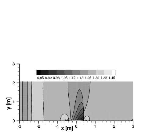
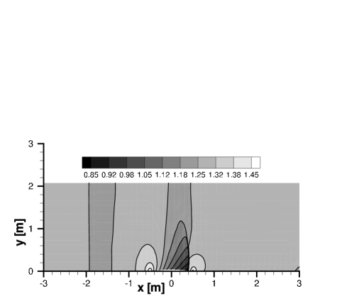
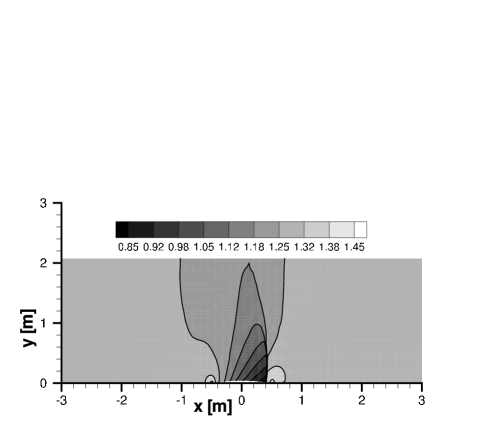
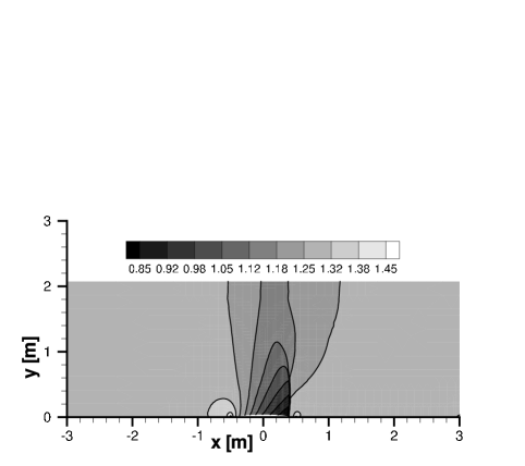
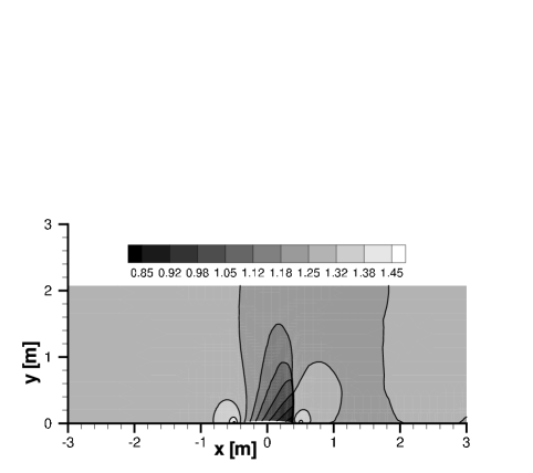
Fig. 8: nonstationary solution of the circular arc bump configuration, uniform timestep $C\!F\!L=1$, level $L=5$, isolines of the density, perturbation entering on the left and leaving on the right side of the computational domain, from top to bottom: $t$ = 0.0057s, 0.00912s, 0.01254s, 0.01596s, 0.01938s.

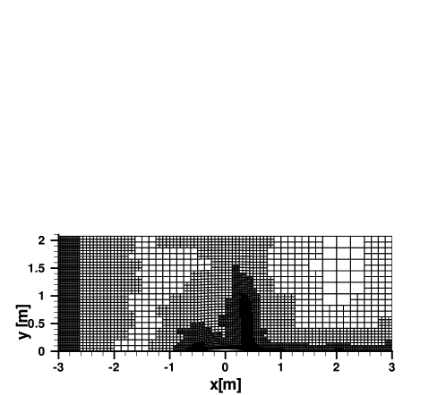
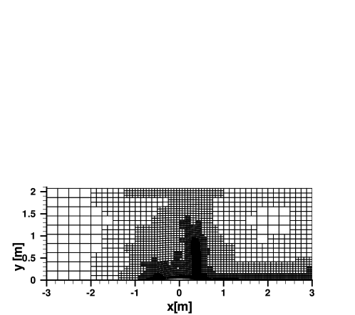
Fig. 9: nonstationary solution of the circular arc bump configuration: adaptive grid $L=5$ for the computation Figure 8, perturbation entering on the left side and leaving on the right side of the computational domain, from top to bottom: $t$ = 0.0057s, 0.00912s, 0.01254s, 0.01596s, 0.01938s.

Remark 7.1.

(i) Our experience is that the averaged pressure is only computed accurately if the whole flow field is well resolved. Therefore our functional-based time adaptation together with the multi resolution spatial adaptation seems to yield a reliable global accuracy both in space and time.

(ii) Note that the functional $J(U)$ is never evaluated because $U$ is not known at all. Instead we compute the localized indicator (46), which involves solving the conservative linearized adjoint problem (41) – (42).

In Figure 8 we show a time-sequence of the nonstationary test case computed with uniform $C\!F\!L=1$ on an adaptive grid with finest level $L=5$. In Figure 9 the corresponding adaptive grids are presented. Note that the perturbation entering at the left boundary and moving through the boundary is resolved very well.

8 Fully implicit computational results

8.1 Numerical strategies

We will present and compare three strategies to demonstrate the efficiency of our space-time adaptive method.

1. Adaptive timesteps via adjoint indicator.
   The first strategy is the one we proposed in [37]: We first compute a forward solution on a coarse grid ($L=2$) and solve the adjoint problem on the adaptive grid of the forward solution. Then we use the information of the error representation based on the dual solution to determine a new sequence of timesteps. This sequence is used in the computation of the forward solution on a grid with finest level $L=5$, where we additionally restrict the $C\!F\!L$ number from below.

2. Adaptive timesteps via ad hoc indicator.
   In the second approach we compare our indicator with ad hoc indicators, which do not require the solution of an adjoint problem. To get these indicators we first do a computation on a coarse grid ($L=2$), and compute residuals in time of the approximate solution.

3. Uniform timesteps.
   In a third approach we will set-up uniform timestep distributions with the same number of timesteps as in the adaptive case of strategy one. We compare the results with our timestep distribution and a uniform in time computation with $C\!F\!L=1$ and $C\!F\!L=10$.

We want to compare these strategies with respect to the following main aspects:

• What is the quality and what are the costs determining the adaptive timestep sequence from computations on the coarse grid?

• Is the predicted adaptive timestep sequence well-adapted to the solution on the fine grid?

• Do ad hoc indicators without computing a dual solution lead to comparable results?

• How is the solution affected if we use uniform timesteps larger than the predicted adaptive timestep sequence?

In order to quantify the results we have to compare with a reference solution. Since the exact solution is not available we perform a computation with $L=5$ refinement levels using implicit timestepping with $C\!F\!L=1$. This is a very expensive approximation for the nonstationary case. For all of the above issues we will discuss the quality of the solution, the computational costs (time and memory) and the efficiency.

8.2 Adaptive timesteps via adjoint indicator

Now we use the error representation on finest level $L=2$ for a new time adaptive computation on finest level $L=5$.

Fig. 10: Time component of the error representation $\bar{\eta}_{k}^{m}$(top) and new timesteps with $C\!F\!L$ restriction from below $C\!F\!L(t_{n})$ (bottom).

The first computation is done on a mesh with finest level $L=2$. We compute until time $T=0.0285s$, which takes 1000 timesteps with $C\!F\!L=1$. We use the results of the error representation of this computation to compute a new timestep distribution. The forward problem takes $329s$ and the dual problem including the evaluation of the error representation $619s$ on an Opteron 8220 processor at 2.86 GHz. The total computational costs are $948s$, and in memory we have to save 1000 solutions (each timestep) of the forward problem which corresponds to 48 MB (total). This gives us a new sequence of adaptive timesteps for the computation of level $L$ = 5. The error indicator and the new timesteps are presented in Figure 10. In time intervals where the solution is stationary, i.e., at the beginning, and after the perturbations have left the computational domain, the timesteps are large. In time intervals where the solution is nonstationary we get well-adapted small timesteps.

Then we use the adaptive timestep sequence for a computation on level $L=5$ and compare it with a uniform in time computation using $C\!F\!L=1$. The uniform computation needs 8000 timesteps and the computational time is $21070s$. The time adaptive solution is computed with 2379 timesteps and this computation takes 9142$s$.

In Figure 12 we show a sequence of plots of the uniform, $C\!F\!L=1$ computation on an adaptive spatial grid with finest level $L=5$. In Figure 13 we compare the pressure distribution at the bottom boundary of the uniform solution and the time adaptive solution at several times. The two solutions on level $L=5$ match very well.

8.3 Adaptive timesteps via ad hoc indicator

Here we replace the adjoint indicator by an ad hoc indicator, which estimates the variation of the solution from one timestep to the following,

$$ind({m})=\sum_{i}|U_{i}^{m}-U_{i}^{m-1}|_{1}|{V_{i}^{m}}|\approx\|U_{h}(\cdot,t^{m})-U_{h}(\cdot,t^{m-1})\|_{L^{1}({\Omega})}.$$ (54)

Clearly this indicates whether the solution is stationary or not. Even though we do not know any theoretically justified global decay rates of $ind$, and much less of the error, as the timestep is refined, it is reasonable to assume that the local variation in time decays linearly with the timestep. Similarly as for the adjoint error control, we do a first computation on a coarse grid with finest level $L=2$, where we compute the indicator, see Figure 11. Then we redistribute the timesteps.

The indicator (54) compares as follows to adjoint error indicator (see Figure 11): Both indicators detect stationary and nonstationary time intervalls. The temporal distribution is very similar, but the variation indicator $ind$ leads to considerably more timesteps than the error indicator from the dual approach (3640 vs. 2379). In particular, most timesteps are smaller than in the case with adaptation via adjoint problems. Since the timesteps are restricted from below, it leads to computations which are in general more expensive but not more accurate. Results are not displayed. One advantage may be that we do not need to compute a dual solution, which makes the computation of the variation indicator less expensive. But this is only a small advantage, since we compute the error indicators on a coarse mesh, which takes $619s$ on level $L=2$ for the adjoint approach. If we use the timesteps which we compute from $ind({m})$ and do a time adaptive computation on a grid with finest level $L=5$ then we will not get equally distributed indicators. This holds also true if we do not apply the timestep restriction from below.

We have also implemented some variations of the discrete variation indicator, which lead to similar results. Another approach was to choose the maximum jump of the solution in one cell, both weighted and not weighted with the size of the cell. This was an approximation to the $L^{\infty}$-norm. This indicator is not very useful, since it turned out to be highly oscillating. Therefore we do not present results for this indicator.

Fig. 11: Comparison of error indicators (top) and timestep sequences (bottom) derived from error representation via dual problem (dashed line) and from variation indicator $ind$ (bold line).

8.4 Uniform timesteps

In many nonstationary computations where no a priori information is known, one reasonable choice is to use uniform $C\!F\!L$ numbers. Therefore we will compare the computation with adaptive implicit timesteps with implicit computations using uniform $C\!F\!L$ numbers. In Section 8.2 we have already done a computation with uniform $C\!F\!L$ number, $C\!F\!L=1$, on a grid with $L=2$, to get timestep sizes for an adaptive computation on a grid with $L=5$. As a reference solution we also computed with uniform $C\!F\!L$ number, $C\!F\!L=1$, a solution of the problem on a grid with $L=5$. Now we compare these computations with computations using higher uniform $C\!F\!L$ numbers.

Fig. 12: Reference solution for 2D Euler equations: adaptive spatial grid (finest level $L=5$), uniform time steps ($C\!F\!L=1$). Pressure $p$ at bottom boundary at times $t$=0.005002, 0.007125, 0.009990, 0.011975, from top to bottom.

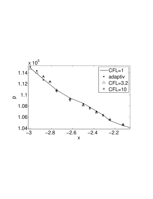
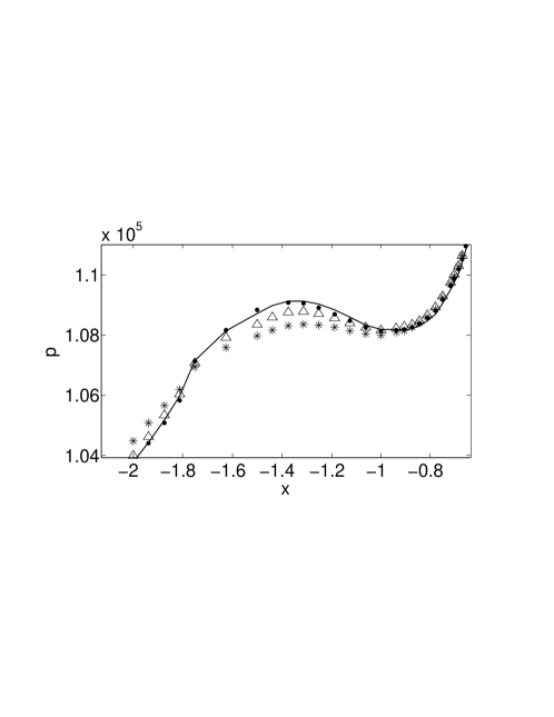
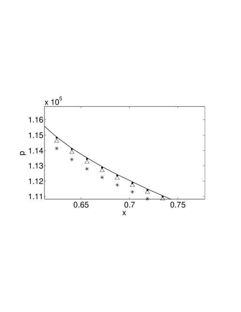
Fig. 13: Zoom tracing the perturbations in Figure 12 at times $t$=0.005002, 0.007125, 0.009990, 0.011975, from top to bottom. Comparison of uniform timesteps with $C\!F\!L=1,\;3.2,\;10$ and time-adaptive strategy.

First we choose a uniform $C\!F\!L$ number of approximately 3.2, which corresponds to 2500 timesteps. This equals roughly the number of timesteps in the adaptive method, and hence it should give a fair comparison. The uniform computation takes about $11509s$, more than the $9142s$ of the adaptive computation (see Table 2). In the uniform computation most of the timesteps are more expensive, since they need more Newton steps, and more steps for solving the linear problems. This shows that the understanding of the dynamics of the solution pays directly in the nonlinear and linear solvers. Moreover, it can be seen from Figure 13 that the quality of the solution is considerably worse than for the adaptive computation.

Another computation with $C\!F\!L$ number 10 takes only $3290s$. However, as can be seen from Figure 13 the solution is badly approximated: In the beginning of the computation the solutions of the different methods match very well, which means that the inflow at the boundary is well-resolved. As time goes on, the solutions differ more and more. After the perturbation has passed the bump, the perturbations differ strongly. Only the time-adaptive method approximates the reference solution ($C\!F\!L=1$) closely.

8.5 Newton iterations and linear iterations

In Figure 14 we show the number of Newton iterations in each timestep for the computations in Section 8.2, 8.3 and 8.4. The number of Newton iterations depend on the $C\!F\!L$ number and is larger, where the solution is nonstationary and smaller, where the solution is stationary. The time-adaptive computation gives the smallest total number of Newton iterations, see Table 2, since most timesteps are solved with one Newton iteration.

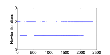
(a) adaptive $C\!F\!L$

(b) $C\!F\!L=1$

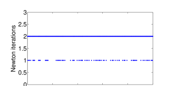
(c) $C\!F\!L\approx$3.2

(d) $C\!F\!L=10$

Fig. 14: Number of Newton iterations for fully implicit time-adaptive computation and computations with uniform $C\!F\!L$ number

Figure 15 shows the total number of linear iterations in each timestep for the same computations, i.e., the sum of the linear iterations in each timestep for all Newton iterations. The number of linear iterations also depends on the $C\!F\!L$ number, for larger $C\!F\!L$ number, we observe more linear iterations.

(a) adaptive $C\!F\!L$

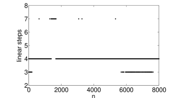
(b) $C\!F\!L=1$

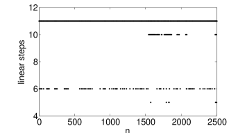
(c) $C\!F\!L\approx$3.2

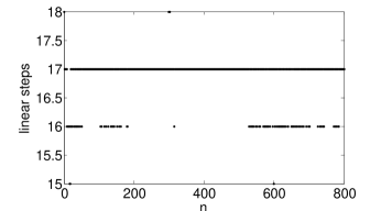
(d) $C\!F\!L=10$

Fig. 15: Number of linear iterations for fully implicit time-adaptive computation and computations with uniform $C\!F\!L$ number

Table 2 gives an overview of the CPU time and the number of Newton iterations and linear iterations for the computations. The costs for the computation of the indicators, both the dual and the ad hoc indicator, on level $L=2$ are very low compared to the costs of computations on level $L=5$. An adaptive computation including the computation of the indicator, i.e., $329s+619s+9142s$, is cheaper than the computation using uniform $C\!F\!L$ number, e.g., $C\!F\!L=1$, that needs 21070$s$. Even the computation with $C\!F\!L=3.2$ is more expensive than the time-adaptive computation, but leads to worse results, see Figure 13.

Table 2 shows that the CPU time is roughly proportional to the number of Newton iterations and not to the number of timesteps or linear solver steps. The CPU time is about $2.5s$ per Newton iteration. This means that we have to minimize the number of Newton iterations in total to accelerate the computation. This is done very efficiently by the time-adaptive approach. For a large range of $C\!F\!L$ numbers from 1 to more than 100, it needs only one or two Newton iterations per timestep, without sacrificing the accuracy.

In this example, the stationary time intervalls are not very large compared to the overall computation. If the stationary time intervalls were larger, the advantage of the time adaptive scheme would be even more significant.

	CPU [s]	timesteps	Newton steps	linear steps
adaptive timesteps	9142	2379	3303	16875
uniform $C\!F\!L=1$	21070	8000	8282	32630
uniform $C\!F\!L=3.2$	11509	2500	4904	26895
uniform $C\!F\!L=10$	3290	800	1600	13500

Table 2: Performance for computations on $L=5$ using different fully implicit timestepping strategies.

9 Explicit-implicit computational results

Now we modify the fully implicit timestepping strategy and introduce a mixed explicit-implicit approach. The reason is that implicit timesteps with $C\!F\!L<5$ are not efficient, since we have to solve a nonlinear system of equations at each timestep. Thus, for $C\!F\!L<5$, the new explicit-implicit strategy switches to the cheaper and less dissipative explicit method with $C\!F\!L=0.5$. The timestep sequence is shown in Figure 16. Of course, we could choose variants of the thresholds $C\!F\!L=0.5$ and 5.

As we can see in Table 3, the new strategy requires 5802 timesteps, where $95\%$ are explicit. The CPU time of $7730s$ easily beats the fully explicit solver ($18702s$), and is also superior to the fully implicit adaptive scheme ($9142s$, see Table 2). The computational results are presented in Figure 17. The results of the combined explicit-implicit strategy are very close to the results of the fully explicit method, and far superior to all fully implicit methods. Note that the explicit scheme serves as reference solution, since it is well-known that it gives the most accurate solution for an nonstationary problem.

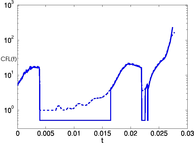
Fig. 16: 2D Euler equations, comparison of timestep sequence derived from error representation for implicit computation (dashed line) and for mixed explicit-implicit computation (bold line).

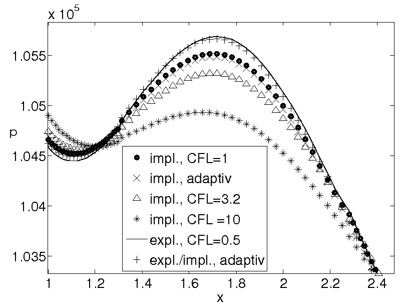
Fig. 17: 2D Euler equations, comparison of solutions in time on adaptive grid with finest level $L=5$, pressure $p$ at the bottom boundary, zoom of the perturbation at time $t$=0.011975

	CPU [s]	timesteps	timesteps
		(total)	(implicit)
explicit $C\!F\!L=0.5$	18702	16000	-
adaptive expl.-impl.	7730	5802	259

Table 3: Performance for computations on $L=5$ using fully explicit timesteps and the time-adaptive explicit-implicit strategy.

10 Conclusion

In this work, explicit and implicit finite volume solvers on adaptively refined quadtree meshes have been coupled with adjoint techniques to control the timestep sizes for the solution of weakly nonstationary compressible inviscid flow problems.

For the 2D Euler equations we have presented a test case for which the time-adaptive method does reach its goals: it separates stationary time intervalls and perturbations cleanly and chooses just the right timestep for each of them. The adaptive method leads to considerable savings in CPU time and memory while reproducing the reference solution almost perfectly.

We have compared the adjoint error representation with several variation-based indicators. Our prime choice is the adjoint approach, since it has the best theoretical justification and needs only half the number of timesteps.

In Theorem 2 and Corollary 3 we state a complete error representation for nonlinear initial-boundary-value problems with characteristic boundary conditions for hyperbolic systems of conservation laws, which includes boundary and linearization errors. Besides building upon well-established adjoint techniques, we also add a new ingredient which simplifies the computation of the dual problem [37]. We show that it is sufficient to compute the spatial gradient of the dual solution, $w=\nabla\varphi$, instead of the dual solution $\varphi$ itself. This gradient satisfies a conservation law instead of a transport equation, and it can therefore be computed with the same algorithm as the forward problem. For discontinuous transport coefficients, the new conservative algorithm for $w$ is more robust than transport schemes for $\varphi$, see [37]. Here we also derive characteristic boundary conditions for the conservative dual problem, which we use in the numerical examples in Sections 8 and 9.

In order to compute the adjoint error representation one needs to compute a forward and a dual problem and to assemble the space-time scalar product (46). Together, this costs about three times as much as the computation of a single forward problem. In our application, the error representation is computed on a coarse mesh ($L=2$), and therefore it presents only a minor computational overhead compared with the fine grid solution ($L=5$). In other applications, the amount of additional storage and CPU time may become significant. In such cases, checkpointing strategies might help (see, e.g., [38]).

We have implemented and tested both a fully implicit and a mixed explicit-implicit timestepping strategy. The explicit-implicit approach switches to an explicit timestep with $C\!F\!L=0.5$ in case the adaptive strategy suggests an implicit timestep with $C\!F\!L<5$. Clearly, the mixed explicit-implicit strategy is the most accurate and efficient, beating the adaptive fully implicit in accuracy and efficiency, the implicit approach with fixed $C\!F\!L$ numbers in accuracy, and the fully explicit approach in efficiency.

Finally, we would like to stress that the computational cost in each timestep is nearly constant, no matter if the $C\!F\!L$ number is of order 1 or order 100. In all cases, the solver needs only 1 or 2 Newton iterations per timestep to reach the (rather strict) break condition, which is related to the multi resolution decomposition. This seems to be another major benefit of the adaptive timestep control.

References

- [1] T.J. Barth and M.G. Larson, A posteriori error estimates for higher order Godunov finite volume methods on unstructured meshes, in Finite volumes for complex applications, III (Porquerolles, 2002), Hermes Sci. Publ., Paris, 2002, pp. 27–49.
- [2] R. Becker and R. Rannacher, A feed-back approach to error control in finite element methods: basic analysis and examples, East-West J. Numer. Math., 4 (1996), pp. 237–264.
- [3] , An optimal control approach to a posteriori error estimation in finite element methods, Acta Numer., 10 (2001), pp. 1–102.
- [4] Marsha J. Berger and Joseph Oliger, Adaptive mesh refinement for hyperbolic partial differential equations, J. Comput. Phys., 53 (1984), pp. 484–512.
- [5] Jürgen Bey and Gabriel Wittum, Downwind numbering: robust multigrid for convection—diffusion problems, Appl. Numer. Math., 23 (1997), pp. 177–192.
- [6] F. Bramkamp, Ph. Lamby, and S. Müller, An adaptive multiscale finite volume solver for unsteady and steady state flow computations, J. Comput. Phys., 197 (2004), pp. 460–490.
- [7] J. M. Carnicer, W. Dahmen, and J. M. Peña, Local decomposition of refinable spaces and wavelets, Appl. Comput. Harmon. Anal., 3 (1996), pp. 127–153.
- [8] CLAWPACK, Conservation law package, http://www.amath.washington.edu/ claw/, (1998).
- [9] A. Cohen, I. Daubechies, and J.-C. Feauveau, Biorthogonal bases of compactly supported wavelets, Comm. Pure Appl. Math., 45 (1992), pp. 485–560.
- [10] A. Cohen, S.M. Kaber, S. Müller, and M. Postel, Fully adaptive multiresolution finite volume schemes for conservation laws, Math. Comp., 72 (2003), pp. 183–225 (electronic).
- [11] R. Courant, K. Friedrichs, and H. Lewy, Über die partiellen Differenzengleichungen der mathematischen physik, Math. Ann., 100 (1928), pp. 32–74.
- [12] Clint Dawson and Robert Kirby, High resolution schemes for conservation laws with locally varying time steps, SIAM J. Sci. Comput., 22 (2000), pp. 2256–2281 (electronic).
- [13] C. De Lellis and L. Szekelyhidi, On admissibility criteria for weak solutions of the euler, Preprint 01-08, Universität Zürich, http://arxiv.org/abs/0712.3288, (2008), pp. 1–33.
- [14] M.O. Domingues, S.M. Gomes, O. Roussel, and K. Schneider, An adaptive multiresolution scheme with local time stepping for evolutionary PDEs, J. Comput. Phys., 227 (2008), pp. 3758–3780.
- [15] M.O. Domingues, O. Roussel, and K. Schneider, On space-time adaptive schemes for the numerical solution of PDEs, in CEMRACS 2005—computational aeroacoustics and computational fluid dynamics in turbulent flows, vol. 16 of ESAIM Proc., EDP Sci., Les Ulis, 2007, pp. 181–194.
- [16] K. Eriksson and C. Johnson, Adaptive finite element methods for parabolic problems. IV. Nonlinear problems, SIAM J. Numer. Anal., 32 (1995), pp. 1729–1749.
- [17] L. Ferm and P. Lötstedt, Space-time adaptive solution of first order PDEs, J. Sci. Comput., 26 (2006), pp. 83–110.
- [18] K. O. Friedrichs and P. D. Lax, Boundary value problems for first order operators, Comm. Pure Appl. Math., 18 (1965), pp. 355–388.
- [19] B. Gottschlich-Müller and S. Müller, Adaptive finite volume schemes for conservation laws based on local multiresolution techniques, in Hyperbolic problems: theory, numerics, applications, Vol. I (Zürich, 1998), vol. 129 of Internat. Ser. Numer. Math., Birkhäuser, Basel, 1999, pp. 385–394.
- [20] A. Harten, Multiresolution representation of data: a general framework, SIAM J. Numer. Anal., 33 (1996), pp. 1205–1256.
- [21] R. Hartmann, A posteriori Fehlerschätzung und adaptive Schrittweiten- und Ortsgittersteuerung bei Galerkin-Verfahren für die Wärmeleitungsgleichung, master’s thesis, Universität Heidelberg, 1998.
- [22] R. Hartmann and P. Houston, Adaptive discontinuous Galerkin finite element methods for nonlinear hyperbolic conservation laws, SIAM J. Sci. Comput., 24 (2002), pp. 979–1004.
- [23] , Adaptive discontinuous Galerkin finite element methods for the compressible Euler equations, J. Comput. Phys., 183 (2002), pp. 508–532.
- [24] H.-O. Kreiss and J. Lorenz, Initial-boundary value problems and the Navier-Stokes equations, vol. 47 of Classics in Applied Mathematics, Society for Industrial and Applied Mathematics (SIAM), Philadelphia, PA, 2004. Reprint of the 1989 edition.
- [25] D. Kröner and M. Ohlberger, A posteriori error estimates for upwind finite volume schemes for nonlinear conservation laws in multidimensions, Math. Comp., 69 (2000), pp. 25–39.
- [26] P. Lamby, Parametric Multi-Block Grid Generation and Application to Adaptive Flow Simulations, PhD thesis, RWTH Aachen University, Germany, 2007.
- [27] Peter D. Lax, Development of singularities of solutions of nonlinear hyperbolic partial differential equations, J. Mathematical Phys., 5 (1964), pp. 611–613.
- [28] S. Müller, Adaptive multiscale schemes for conservation laws, vol. 27 of Lecture Notes in Computational Science and Engineering, Springer-Verlag, Berlin, 2003.
- [29] Siegfried Müller and Youssef Stiriba, Fully adaptive multiscale schemes for conservation laws employing locally varying time stepping, J. Sci. Comput., 30 (2007), pp. 493–531.
- [30] M. Ohlberger, A posteriori error estimate for finite volume approximations to singularly perturbed nonlinear convection-diffusion equations, Numer. Math., 87 (2001), pp. 737–761.
- [31] O. A. Oleĭnik, Discontinuous solutions of non-linear differential equations, Amer. Math. Soc. Transl. (2), 26 (1963), pp. 95–172.
- [32] B. Pollul, Iterative Solvers in Implicit Time Integration for Compressible Flows, PhD thesis, RWTH Aachen University, Germany, 2008.
- [33] A. Rizzi and H. Viviand, eds., Numerical methods for the computation of inviscid transonic flows with shock waves, vol. 3 of Notes on Numerical Fluid Mechanics, Friedr. Vieweg & Sohn, Braunschweig, 1981.
- [34] P. L. Roe, Approximate Riemann solvers, parameter vectors, and difference schemes, J. Comput. Phys., 43 (1981), pp. 357–372.
- [35] Youcef Saad and Martin H Schultz, Gmres: a generalized minimal residual algorithm for solving nonsymmetric linear systems, SIAM J. Sci. Stat. Comput., 7 (1986), pp. 856–869.
- [36] Thomas C. Sideris, Formation of singularities in solutions to nonlinear hyperbolic equations, Arch. Rational Mech. Anal., 86 (1984), pp. 369–381.
- [37] C. Steiner and S. Noelle, On adaptive timestepping for weakly instationary solutions of hyperbolic conservation laws via adjoint error control, Comm. Numer. Meth. Eng., doi:10.1002/cnm.1183, (2008).
- [38] J. Sternberg and A. Griewank, Reduction of storage requirement by checkpointing for time-dependent optimal control problems in ODEs, in Automatic differentiation: applications, theory, and implementations, vol. 50 of Lect. Notes Comput. Sci. Eng., Springer, Berlin, 2006, pp. 99–110.
- [39] E. Süli, A posteriori error analysis and adaptivity for finite element approximations of hyperbolic problems, in An introduction to recent developments in theory and numerics for conservation laws (Freiburg/Littenweiler, 1997), vol. 5 of Lect. Notes Comput. Sci. Eng., Springer, Berlin, 1999, pp. 123–194.
- [40] E. Süli and P. Houston, Adaptive finite element approximation of hyperbolic problems, in Error estimation and adaptive discretization methods in computational fluid dynamics, vol. 25 of Lect. Notes Comput. Sci. Eng., Springer, Berlin, 2003, pp. 269–344.
- [41] E. Tadmor, Local error estimates for discontinuous solutions of nonlinear hyperbolic equations, SIAM J. Numer. Anal., 28 (1991), pp. 891–906.