Band gaps in the relaxed linear micromorphic continuum

Abstract

In this note we show that the relaxed linear micromorphic model recently proposed by the authors can be suitably used to describe the presence of band-gaps in metamaterials with microstructures in which strong contrasts of the mechanical properties are present (e.g. phononic crystals and lattice structures). This relaxed micromorphic model only has 6 constitutive parameters instead of 18 parameters needed in Mindlin- and Eringen-type classical micromorphic models. We show that the onset of band-gaps is related to a unique constitutive parameter, the Cosserat couple modulus $\mu_{c}$ which starts to account for band-gaps when reaching a suitable threshold value. The limited number of parameters of our model, as well as the specific effect of some of them on wave propagation can be seen as an important step towards indirect measurement campaigns.

1. Université de Lyon-INSA, 20 Av. Albert Einstein, 69100 Villeurbanne Cedex, France.

2. Lehrstuhl für Nichtlineare Analysis und Modellierung, Fakultät für Mathematik, Universität Duisburg-Essen, Campus Essen, Thea-Leymann Str. 9, 45127 Essen, Germany.

3. Dep. of Mathematics, University “A.I. Cuza”, 11 Blvd. Carol I, Ia̧si; Octav Mayer Institute of Mathematics, Romanian Academy, Ia̧si; Institute of Solid Mechanics, Romanian Academy, Bucharest, Romania.

4. Università Telematica Internazionale Uninettuno, Corso V. Emanuele II 39, 00186 Roma, Italy.

5. Laboratoire Modélisation Multi Echelle, MSME UMR 8208 CNRS, Université Paris-Est, 61 Avenue du Géneral de Gaulle, Créteil Cedex 94010, France.

6. International Research Center for the Mathematics and Mechanics of Complex Systems (M&MoCS), Università dell’Aquila, Palazzo Caetani, 04012 Cisterna di Latina, Italia

1 Introduction

Micromorphic models were originally proposed by Mindlin [23] and Eringen [5] in order to study materials with microstructure while remaining in the simplified framework of macroscopic continuum theories. Nevertheless, the huge number of material parameters (18 in the linear-isotropic case) limited up to now the application of these powerful theories to describe the behavior of real metamaterials (see e.g. [25]). In this paper, we propose to use the newly developed relaxed micromorphic model presented in [6, 26] to study wave propagation in microstructured materials which exhibit frequency band-gaps. In the present paper we want to focus on a new and fascinating development in generalized continuum models applied to band-gaps wave phenomena. In a companion paper [15] we have detailed how the proposed relaxed model can be compared with classical micromorphic and with second gradient and Cosserat models. Here, we mainly summarize our results concerning the description of frequency band-gaps in relaxed micromorphic continua and we detail how the effect of the Cosserat couple modulus $\mu_{c}$ is essential for their description.

The proposed relaxed model only counts six constitutive parameters and is fully able to account for the effect of microstructure on the macroscopic mechanical behavior of the considered media. The request of positive-definiteness for the proposed relaxed model is weaker with respect to the classical Mindlin-Eringen model (positive-definiteness of the energy with the whole gradient term). This weaker request allows the relaxed model to account for weaker connections at the microscopic level compared to those which are possible in classical micromorphic theories. For this reason the proposed relaxed model allows the description of band gaps while the classical approach does not.

It is known that some materials like phononic crystals and lattice structures (see e.g. [30]), granular assemblies with defects (see e.g. [11, 19, 20, 21]) and composites ([4, 31]) can inhibit wave propagation in particular frequency ranges (band-gaps). The aim of this note is to show that the proposed relaxed model allows for describing frequency band-gaps by “switching on” a unique constitutive parameter which is known as Cosserat couple modulus $\mu_{c}$ (see e.g. [9, 10, 24, 27, 28]). The limited number of constitutive parameters makes possible the future conception of direct and indirect measurements on real materials exhibiting frequency band-gaps. On the other hand, the generality of the proposed relaxed model can also be seen as a tool to aid the engineering design of new metamaterials with improved band-gap capabilities. Materials of this type could be used as an alternative to piezoelectric materials which are used today for vibration control and which are for this reason extensively studied in the literature (see e.g. [1, 3, 17, 18, 29, 32]). Because of the possible interest of our findings in a linear modelling framework, we summarize in this communication the main novel results on band gaps related to our relaxed micromorphic model.

2 Equations of motion in strong form

As shown in [26] the equations of motion of the considered linear relaxed isotropic and homogeneous micromorphic continuum, when neglecting body loads, read

$$\rho\,\mathbf{u}_{tt}= \mathrm{Div}\left[2\,\mu_{e}\,\mathrm{sym}\left(\nabla\mathbf{u}-\mathbf{P}\right)+\lambda_{e}\mathrm{tr}\left(\nabla\mathbf{u}-\mathbf{P}\right)\mathds{1}+2\,\mu_{c}\,\mathrm{skew}\left(\nabla\mathbf{u}-\mathbf{P}\right)\right]$$

$$\eta\,\mathbf{P}_{tt}= -\alpha_{c}\,\mathrm{\mathrm{Cur}l}\left(\mathrm{\mathrm{Cur}l}\,\mathbf{P}\right)+2\,\mu_{e}\,\mathrm{sym}\left(\nabla\mathbf{u}-\mathbf{P}\right)+\lambda_{e}\mathrm{tr}\left(\nabla\mathbf{u}-\mathbf{P}\right)\mathds{1}$$

$$-2\,\mu_{h}\,\mathrm{sym}\,\mathbf{P}-\lambda_{h}\mathrm{tr}\,\mathbf{P}\>\mathds{1}+2\,\mu_{c}\,\mathrm{skew}\left(\nabla\mathbf{u}-\mathbf{P}\right),$$

where $\mathbf{u}\in\mathbb{R}^{3}$ is the displacement field, $\mathbf{P}\in\mathbb{R}^{3\times 3}$ is the microdeformation tensor (basic kinematical fields), $\rho$ and $\eta$ are the macro and micro mass densities respectively and all other quantities are the constitutive parameters of the model. As for the operators appearing in (LABEL:eq:bulk-mod-3), we use the following notations

$$\mathrm{sym}\,\mathbf{X}=\frac{\mathbf{X}+\mathbf{X}^{T}}{2}\qquad\mathrm{skew}\,\mathbf{X}=\frac{\mathbf{X}-\mathbf{X}^{T}}{2},\qquad\mathrm{tr}\,\mathbf{X}=X_{ii},$$

$$(\mathrm{Div}\,\mathbf{X})_{i}=X_{ij,j},\qquad\left(\nabla\mathbf{u}\right)_{ij}=u_{i,j},\qquad(\mathrm{Curl}\>\mathbf{X}_{ij}=X_{ia,b}\epsilon_{jab}),$$

where $\epsilon_{jab}$ is the classical Levi-Civita symbol, $X_{ij}$ denote the components of the tensor $\mathbf{X}$, the subscript $t$ indicates a time deivative, the subscript $j$ indicates the derivative with respect to the $j$-th component of the space variable and the Einstein summation convention over repeated indices has been adopted. It can be checked that when considering a completely one-dimensional case, the term $\mathrm{\mathrm{Cur}l}\left(\mathrm{\mathrm{Cur}l}\,\mathbf{P}\right)$ vanishes and no characteristic length related to microstructure can be accounted for by our model. We need at least the case of plane waves (all the components of $\mathbf{u}$ and $\mathbf{P}$ are non-vanishing, but all depend on one space variable $X$ which is also the direction of propagation of considered wave) to disclose all the characteristic features of the proposed relaxed model. On the other hand, the Mindlin-Eringen models allow to account for characteristic lengths even when considering complete one-dimensional cases (all components of the kinematical fields in the plane orthogonal to the direction of propagation are vanishing). This is shown e.g. in [2, 16] in which these fully 1D equations are derived by the standard internal variable theory. We also remark that, in general, the relaxed term $\mathrm{\mathrm{Cur}l}\left(\mathrm{\mathrm{Cur}l}\,\mathbf{P}\right)$ in the second of Eqs. (LABEL:eq:bulk-mod-3) is much weaker than the full term $\Delta\mathbf{P}$ appearing in Mindlin- and Eringen-type models. Despite this weaker formulation, we claim that the proposed relaxed model is fully able to account for the presence of microstructure on the overall mechanical behavior of the considered continua. In particular, our relaxed model is able to account for the description of frequency band-gaps, while the classical Mindlin- and Eringen-type models are not.

In [26] it is also proved that positive definiteness of the strain energy density associated to Eqs.(LABEL:eq:bulk-mod-3) implies

$$\mu_{e}>0,\quad\mu_{c}\geq 0,\quad 3\lambda_{e}+2\mu_{e}>0,\quad\mu_{h}>0,\quad 3\lambda_{h}+2\mu_{h}>0,\quad\alpha_{c}>0$$ (2)

In this note we will only consider non-vanishing, positive values of the Cosserat couple modulus $\mu_{c}$ which is seen as a trigger of the band-gap phenomenon.

We limit ourselves to the case of plane waves travelling in an infinite domain, i.e. we suppose that the space dependence of all the introduced kinematical fields is limited only to the space component $X$ which we also suppose to be the direction of propagation of the considered wave. We introduce the new variables

$$P^{S}:=\frac{1}{3}\left(P_{11}+P_{22}+P_{33}\right),\quad P^{D}:=\left(\mathrm{dev\>sym}\,\mathbf{P}\right)_{11},$$

$$P_{(1\xi)}:=\left(\mathrm{sym}\>\mathbf{P}\right)_{1\xi},\quad P_{\left[1\xi\right]}:=\left(\mathrm{skew}\>\mathbf{P}\right)_{1\xi},\quad\xi=1,2.$$

It is immediate that, according to the Cartan-Lie-algebra decomposition (see e.g. [26]), the component $P_{11}$ of the tensor $\mathbf{P}$ can be rewritten as $P_{11}=P^{D}+P^{S}$. We also define the additional variables

$$P^{V}=P_{22}-P_{33},\qquad P_{(1\xi)}=\left(\mathrm{sym}\>\mathbf{P}\right)_{1\xi},\qquad P_{\left[1\xi\right]}=\left(\mathrm{skew}\>\mathbf{P}\right)_{1\xi},\quad\xi=1,2.$$ (4)

We rewrite the equations of motion (LABEL:eq:bulk-mod-3) in terms of the new variables (LABEL:SpherDev), (4) and, of course, of the displacement variables. Before doing so, we introduce the quantities

$$c_{m}=\sqrt{\frac{\alpha_{c}}{\eta}},\qquad c_{s}=\sqrt{\frac{\mu_{e}+\mu_{c}}{\rho}},\qquad c_{p}=\sqrt{\frac{\lambda_{e}+2\mu_{e}}{\rho}},$$

$$\omega_{s}=\sqrt{\frac{2\left(\mu_{e}+\mu_{h}\right)}{\eta}},\quad\omega_{p}=\sqrt{\frac{\left(3\lambda_{e}+2\mu_{e}\right)+\left(3\lambda_{h}+2\mu_{h}\right)}{\eta}},\quad\omega_{r}=\sqrt{\frac{2\mu_{c}}{\eta}},$$ (5)

$$\omega_{l}=\sqrt{\frac{\lambda_{h}+2\mu_{h}}{\eta}},\quad\omega_{t}=\sqrt{\frac{\mu_{h}}{\eta}}.$$

With the proposed new choice of variables and recalling that we are considering the case of planar waves, we are able to rewrite the governing equations (LABEL:eq:bulk-mod-3) as different uncoupled sets of equations, namely:

• A set of three equations only involving longitudinal quantities (left) and two sets of three equations only involving transverse quantities in the $k$-th direction:

$$\begin{cases}\ddot{u}_{1}=c_{p}^{2}u_{1,11}-\frac{2\mu_{e}}{\rho}\,P_{,1}^{D}-\frac{3\lambda_{e}+2\mu_{e}}{\rho}\,P_{,1}^{S},\\ \\ \ddot{P}^{D}=\frac{4}{3}\,\frac{\mu_{e}}{\eta}u_{1,1}+\frac{1}{3}c_{m}^{2}P_{,11}^{D}-\frac{2}{3}c_{m}^{2}P_{,11}^{S}-\omega_{s}^{2}P^{D},\\ \\ \ddot{P}^{S}=\frac{3\lambda_{e}+2\mu_{e}}{3\eta}u_{1,1}-\frac{1}{3}c_{m}^{2}P_{,11}^{D}+\frac{2}{3}c_{m}^{2}P_{,11}^{S}-\omega_{p}^{2}P^{S},\end{cases}$$

$$\begin{cases}\ddot{u}_{\xi}=c_{s}^{2}u_{\xi,11}-\frac{2\mu_{e}}{\rho}\,P_{\left(1\xi\right),1}+\frac{\eta}{\rho}\omega_{r}^{2}P_{\left[1\xi\right],1},\\ \\ \ddot{P}_{\left(1\xi\right)}=\frac{\mu_{e}}{\eta}u_{\xi,1}+\frac{1}{2}c_{m}^{2}P_{(1\xi)}{}_{,11}+\frac{1}{2}c_{m}^{2}P_{\left[1\xi\right],11}-\omega_{s}^{2}P_{(1\xi)},\\ \\ \ddot{P}_{\left[1\xi\right]}=-\frac{1}{2}\omega_{r}^{2}u_{\xi,1}+\frac{1}{2}c_{m}^{2}P_{(1\xi),11}+\frac{1}{2}c_{m}^{2}P_{\left[1\xi\right]}{}_{,11}-\omega_{r}^{2}P_{\left[1\xi\right]},\end{cases}$$

, with $\xi=2,3$.

• Three uncoupled equations only involving the variables $P_{\left(23\right)}$, $P_{\left[23\right]}$ and $P^{V}$ respectively

$$\ddot{P}_{\left(23\right)}=-\omega_{s}^{2}P_{\left(23\right)}+c_{m}^{2}P_{\left(23\right),11},\quad\ddot{P}_{\left[23\right]}=-\omega_{r}^{2}P_{\left[23\right]}+c_{m}^{2}P_{\left[23\right],11},$$

$$\ddot{P}^{V}=-\omega_{s}^{2}P^{V}+c_{m}^{2}P_{,11}^{V}.$$

These 12 scalar differential equations will be used to study wave propagation in our relaxed micromorphic media.

3 Plane wave propagation

We now look for a wave form solution of the previously derived equations of motion. We start from the uncoupled Eqs. (LABEL:Shear) and assume that the involved unknown variables take the harmonic form

$$P_{\left(23\right)}=Re\left\{\beta_{\left(23\right)}e^{i(kX-\omega t)}\right\},\quad P_{\left[23\right]}=Re\left\{\beta_{\left[23\right]}e^{i(kX-\omega t)}\right\},$$

$$P^{V}=Re\left\{\beta^{V}e^{i(kX-\omega t)}\right\},$$

where $\beta_{\left(23\right)}$, $\beta_{\left[23\right]}$ and $\beta^{V}$ are the amplitudes of the three introduced waves. Replacing this wave form in Eqs. (LABEL:Shear) and simplifying one obtains the following dispersion relations respectively:

$$\omega(k)=\sqrt{\omega_{s}^{2}+k^{2}c_{m}^{2}},\qquad\omega(k)=\sqrt{\omega_{r}^{2}+k^{2}c_{m}^{2}},\qquad\omega(k)=\sqrt{\omega_{s}^{2}+k^{2}c_{m}^{2}}.$$ (9)

We notice that for a vanishing wave number ($k=0$) the dispersion relations for the three considered waves give non-vanishing frequencies so that these waves are so-called optic waves with cutoff frequencies $\omega_{s}$, $\omega_{r}$ and $\omega_{s}$ respectively.

We now introduce the unknown vectors $\mathbf{v}_{1}=\left(u_{1},P^{D},P^{S}\right)$ and $\mathbf{v}_{\xi}=\left(u_{\xi},P_{(1\xi)},P_{[1\xi]}\right),\ \xi=2,3$ and look for wave form solutions of equations (LABEL:Longitudinal) in the form

$$\mathbf{v}_{1}=Re\left\{\boldsymbol{\beta}e^{i(kX-\omega t)}\right\},\qquad\mathbf{v}_{\xi}=Re\left\{\boldsymbol{\gamma}^{\xi}e^{i(kX-\omega t)}\right\},\ \xi=2,3,$$ (10)

where $\boldsymbol{\beta}=(\beta_{1},\beta_{2},\beta_{3})^{T}$ and $\boldsymbol{\gamma}^{\xi}=(\gamma_{1}^{\xi},\gamma_{2}^{\xi},\gamma_{3}^{\xi})^{T}$ are the unknown amplitudes of the considered waves. Replacing this expressions in Eqs. (LABEL:Longitudinal) one gets respectively

$$\mathbf{A}_{1}\cdot\boldsymbol{\beta}=0,\qquad\qquad\mathbf{A}_{\xi}\cdot\boldsymbol{\gamma}^{\xi}=0,\qquad\qquad\xi=2,3,$$ (11)

where

$$\mathbf{A}_{1}=\left(\begin{array}[]{ccc}-\omega^{2}+c_{p}^{2}\,k^{2}&\,i\>k\>2\mu_{e}/\rho&i\>k\>\left(3\lambda_{e}+2\mu_{e}\right)/\rho\\ \\ -i\>k\,\frac{4}{3}\,\mu_{e}/\eta&-\omega^{2}+\frac{1}{3}k^{2}c_{m}^{2}+\omega_{s}^{2}&-\frac{2}{3}\,k^{2}c_{m}^{2}\\ \\ -\frac{1}{3}\,i\,k\>\left(3\lambda_{e}+2\mu_{e}\right)/\eta&-\frac{1}{3}\,k^{2}\,c_{m}^{2}&-\omega^{2}+\frac{2}{3}\,k^{2}\,c_{m}^{2}+\omega_{p}^{2}\end{array}\right),$$

$$\mathbf{A}_{2}=\mathbf{A}_{3}=\left(\begin{array}[]{ccc}-\omega^{2}+k^{2}c_{s}^{2}&\,i\,k\,2\mu_{e}/\rho&-i\,k\,\frac{\eta}{\rho}\omega_{r}^{2},\\ \\ -\,i\,k\,2\mu_{e}/\eta,&-2\omega^{2}+k^{2}c_{m}^{2}+2\omega_{s}^{2}&k^{2}c_{m}^{2}\\ \\ i\,k\,\omega_{r}^{2}&k^{2}c_{m}^{2}&-2\omega^{2}+k^{2}c_{m}^{2}+2\omega_{r}^{2}\end{array}\right).$$

In order to have non-trivial solutions of the algebraic systems (11), one must impose that

$$\mathrm{det}\,\mathbf{A}_{1}=0,\qquad\qquad\mathrm{det}\,\mathbf{A}_{2}=0,\qquad\qquad\mathrm{det}\,\mathbf{A}_{3}=0,$$ (12)

which are the so-called dispersion relations $\omega=\omega\left(k\right)$ for the longitudinal and transverse waves in the relaxed micromorphic continuum.

4 Numerical results

In this section, following Mindlin [23, 5], we will show the dispersion relations $\omega=\omega(k)$ associated to our relaxed micromorphic model.

Parameter	Value	Unit	Description
$\lambda$	$82.5$	$MPa$	Macroscopic Lamé modulus
$\mu$	$66.7$	$MPa$	Macroscopic Lamé modulus
$\rho$	$2500$	$Kg/m^{3}$	Macroscopic mass density
$\rho^{\prime}$	$2500$	$Kg/m^{3}$	Microscopic mass density
$\mu_{e}$	$200$	$MPa$	Isotropic scale transition parameter
$\lambda_{e}=2\mu_{e}$	400	$MPa$	Isotropic scale transition parameter
$\lambda_{h}$	$100$	$MPa$	Microscopic Lamé modulus
$\mu_{h}$	100	$MPa$	Microscopic Lamé modulus
$d$	$2$	$mm$	Characteristic size of inclusions
$L_{c}$	$3$	$mm$	Internal length
$\eta=d^{2}\,\rho^{\prime}$	$10^{-2}$	$Kg/m$	Micro-inertia
$\alpha_{c}=\mu_{e}L_{c}^{2}$	$1.8\times 10^{-3}$	$MPa\>m^{2}$	Microscopic stiffness

Table 1: Values of the parameters of the relaxed model used in the numerical simulations.

We start by showing in Tab. 1 the values of the parameters of the relaxed model used in the performed numerical simulations. In order to make the obtained results better exploitable, we also recall that in [26, 25] the following homogenized formulas were obtained which relate the parameters of the relaxed model to the macroscopic Lamé parameters $\lambda$ and $\mu$ which are usually measured by means of standard mechanical tests

$$\mu_{e}=\frac{\mu_{h}\,\mu}{\mu_{h}-\mu},\qquad 2\mu_{e}+3\lambda_{e}=\frac{(2\mu_{h}+3\lambda_{h})\left(2\mu+3\lambda\right)}{(2\mu_{h}+3\lambda_{h})-\left(2\mu+3\lambda\right)}.$$ (13)

These relationships imply that the following inequalities are satisfied: $\mu_{h}>\mu$, $3\lambda_{h}+2\mu_{h}>3\lambda+2\mu$. It is clear that, once the values of the parameters of the relaxed models are known, the standard Lamé parameters can be calculated by means of formulas (13), which is what was done in Tab. 1. The table also includes the values of two characteristic lengths $L_{c}$ and $d$ which can be respectively associated to the characteristic length corresponding to the relaxed micromorphic coefficient $\alpha_{c}$ and to the characteristic size of microscopic inclusions. Indeed, while the parameter $d$ can be directly associated to the size of microstructure (see also [23]), the physical meaning of the parameter $L_{c}$ is more difficult to be visualized. This latter can be indeed associated to the characteristic size of the region of interactions of a Representative Elementary Volume with the surrounding ones. The characteristic length $L_{c}$ can be hence associated, for example, to the size of some particular boundary layers which can be observed in the deformation patterns of micro-structured materials subjected to particular types of loading and/or boundary conditions. Finally, it should be noted that the micro inertia $\eta$ is calculated using the microscopic mass density $\rho$, which is the density of inclusions, as suggested by Mindlin [22].

The numerical values of the parameters listed in Tab. 1 have been chosen in the set of all possible values in order to let band-gaps clearly appear in a frequency range which can be considered to be of physical interest. Indeed, the band gaps which are shown in this paper range between $80$ and $200\,kHz$, which are values proposed for band gaps in phononic crystals (see e.g.[12]). The Young’s modulus of the homogenized material considered in the present paper corresponds to the one of a rather soft material. Nevertheless, stiffer materials can also be considered which still show frequency band-gaps by slightly changing the other involved parameters.

It is evident (see Eqs. (5)) that, in general, the relative positions of the horizontal asymptotes $\omega_{l}$ and $\omega_{t}$ as well as of the cutoff frequencies $\omega_{s}$, $\omega_{r}$ and $\omega_{p}$ can vary depending on the values of the constitutive parameters (see (5)). It can also be checked that, in the case in which $\lambda_{e}>0$ and $\lambda_{h}>0$ one always has $\omega_{p}>\omega_{s}>\omega_{t}$ and $\omega_{l}>\omega_{t}$: we will keep this hypothesis in the remainder of the paper. The relative position of $\omega_{l}$ and of $\omega_{s}$ can vary depending on the values of the parameters $\lambda_{h}$ and $\mu_{h}$. It can be finally recognized that, in order to have a global band-gap, i.e. a frequency range in which no one of the considered types of waves can propagate, the following conditions must be simultaneously satisfied: $\omega_{s}>\omega_{l}$ and $\omega_{r}>\omega_{l}$. In terms of the constitutive parameters of the relaxed model, we can say that global band-gaps can exist, in the case in which one considers positive values for the parameters $\lambda_{e}$ and $\lambda_{h}$ , if and only if we have simultaneously

$$0<\mu_{e}<+\infty,\qquad\qquad 0<\lambda_{h}<2\mu_{e},\qquad\qquad\mu_{c}>\frac{\lambda_{h}+2\text{$\mu$}_{h}}{2}=:\mu_{c}^{0}.$$ (14)

As far as negative values for $\lambda_{e}$ and $\lambda_{h}$ are allowed, the conditions for band gaps are not so straightforward as (14), but we do not consider this possibility in this note. In the numerical simulations presented in this note we choose to test three characteristic values of the Cosserat couple modulus as listed in Tab. 2.

Case	Value	Unit
1	$\mu_{c}=\mu_{c}^{0}=1.5$	$MPa$
2	$\mu_{c}=2\mu_{c}^{0}=3$	$MPa$
3	$\mu_{c}=3\mu_{c}^{0}=4.5$	$MPa$

Table 2: Characteristic values of the Cosserat couple modulus $\mu_{c}$ chosen for the numerical simulations (the values of the parameters $\lambda_{h}$ et $\mu_{h}$ are given in Tab. 1).

The choice of these characteristic values allows to show how the Cosserat couple modulus is indeed the parameter which is responsible for the onset of band-gaps in the considered generalized continuum.

Figure 1 shows the dispersion relations for the considered relaxed micromorphic continuum for the lower bound $\mu_{c}=\mu_{c}^{0}$.

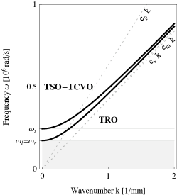
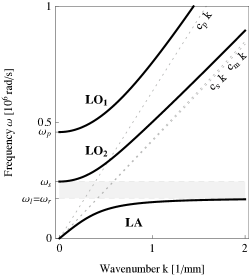
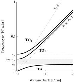
(a)	(b)	(c)

Figure 1: Dispersion relations $\omega=\omega(k)$ for $\mu_{c}=\mu_{c}^{0}$: uncoupled waves (a), longitudinal waves (b) and transverse waves (c). TRO: transverse rotational optic, TSO: transverse shear optic, TCVO: transverse constant-volume optic, LA: longitudinal acoustic, LO₁-LO₂: first and second longitudinal optic, TA: transverse acoustic, TO₁-TO₂: first and second transverse optic.

It can be immediately seen that we cannot identify a frequency band in which overall wave propagation is forbidden. More precisely, for any value of frequency, at least on wave exists (longitudinal, transverse or uncoupled) which propagates inside the considered medium. Things become different as soon as the value of the Cosserat couple modulus increases. In Fig. 2 we show the dispersion relations for the relaxed micromorphic model corresponding to $\mu_{c}=2\,\mu_{c}^{0}$.

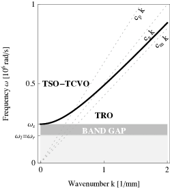
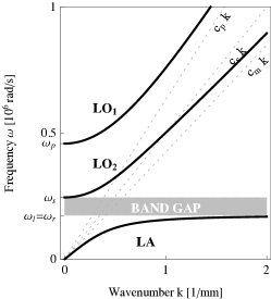
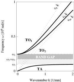
(a)	(b)	(c)

Figure 2: Dispersion relations $\omega=\omega(k)$ for $\mu_{c}=2\>\mu_{c}^{0}$: uncoupled waves (a), longitudinal waves (b) and transverse waves (c). TRO: transverse rotational optic, TSO: transverse shear optic, TCVO: transverse constant-volume optic, LA: longitudinal acoustic, LO₁-LO₂: first and second longitudinal optic, TA: transverse acoustic, TO₁-TO₂: first and second transverse optic.

It can be remarked that in this case any type of wave can propagate in the frequency range $[\omega_{l},\omega_{s}]$, so that we can state that a band-gap can be observed which is actually triggered by the increasing value of the Cosserat couple modulus. In this frequency range the wavenumber becomes imaginary and only standing waves exist. For the sake of completeness, we also show in Fig. 3 a third value for the Cosserat couple modulus, namely $\mu_{c}=3\,\mu_{c}^{0}$.

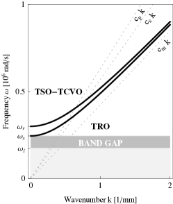
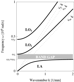
(a)	(b)	(c)

Figure 3: Dispersion relations $\omega=\omega(k)$ for $\mu_{c}=3\,\mu_{c}^{0}$: (a), longitudinal waves (b) and transverse waves (c). TRO: transverse rotational optic, TSO: transverse shear optic, TCVO: transverse constant-volume optic, LA: longitudinal acoustic, LO₁-LO₂: first and second longitudinal optic, TA: transverse acoustic, TO₁-TO₂: first and second transverse optic.

It can be easily noticed from Fig. 3 that the frequency band gap remains unchanged with respect to the previous case, even if the global behavior of the system is much more complicated (two cutoff frequencies for the uncoupled and transverse waves instead than one). We can hence confirm that the presence of band-gaps is actually triggered by the Cosserat couple modulus and we can observe that the wider extension of such band-gaps is reached for $\mu_{c}=2\,\mu_{c}^{0}$.

As shown by Eq. (LABEL:eq:bulk-mod-3), the Cosserat couple modulus is a homogenized elastic coefficient which allows to account for the relative rotation of the microscopic inclusions with respect to the macroscopic matrix. Even if no length scale is associated to this parameter, the fact that the considered microstructure can rotate with respect to the matrix in which it is embedded, actually appears to be a crucial point in order to have the onset of frequency band gaps at the macroscopic level. In[24] it has been demonstrated that the Cosserat couple modulus is zero for continuous materials. Therefore, a positive Cosserat couple modulus accounts for the discreteness of the considered meta-material.

Wave propagation in complex media exhibiting acoustic and optic branches generating frequency band-gaps can be compared to wave propagation in discrete media such as phononic crystals and diatomic chains. The method proposed in this paper allows to account for a homogenized behavior of the considered material, so that the forecasted band-gaps are not directly related to a precise microstructure via a rigorous homogenization procedure. Indeed, the method proposed in the present pape, allows to forecast frequency band gaps in precise ranges of frequency which have been directly associated to particular microstructures (see e.g. [10]). For this reason, the macroscopic method presented here could be of great interest for describing systems with complex microstructures with a very limited number of constitutive parameters.

It is worth noticing that in our relaxed micromorphic model the observed forbidden range of frequency is valid for every plane wave solution (compression and shear). In the papers of Grekova and co-workers [14, 7] the reduced Cosserat medium is analyzed. The reduced Cosserat model can be obtained by our relaxed micromorphic model by setting $\alpha_{c}=0$ and $\mu_{h}\rightarrow\infty$. It is shown that if the reduced Cosserat model is analyzed, the bulk plane compression wave does not change compared with the classical case and band-gaps associated to these waves are not observed, due to the presence of a compressive acoustic wave. On the other hand, the shear wave is strongly influenced by the presence of rotational degrees of freedom and a forbidden range of frequency exists. Seismological observations [8, 13] confirm these theoretical investigations and tell us that near earthquake centers often there are zones absorbing shear waves of a certain band of frequencies. The micromorphic model proposed in the present paper can be considered to be more general with respect to other continuum models which are available in the literature in the sense that global band gaps (compression and shear) can be forecasted.

For what concerns the complete Cosserat model, it can be obtained from our relaxed micromorphic model by simply setting $\mu_{h}\rightarrow\infty$. In this case, no band gaps can be observed at all due to the presence of an acoustic wave both for the compression and for the shear waves.

We conclude by saying that the relaxed micromorphic model proposed in [6, 26] is able to describe the presence of frequency band-gaps in which no wave propagation can occur. The presence of band-gaps is intrinsically related to a critical value of the Cosserat couple modulus $\mu_{c}$ (see [9, 10, 24, 27, 28] for its interpretation) which must be greater than a threshold value in order to let band-gaps appear. This parameter can hence be seen as a discreteness quantifier which starts accounting for lattice discreteness as soon as it reaches the threshold value specified in Eq.(14). This fact is a novel feature of the introduced relaxed model: we claim that neither the classical micromorphic continuum model nor the Cosserat and the second gradient ones are able to predict such band-gap phenomena.

References

- [1] U. Andreaus, F. dell’Isola, and M. Porfiri. Piezoelectric passive distributed controllers for beam flexural vibrations. Journal of Vibration and Control, 10(5):625–659, 2004.
- [2] A. Berezovski, J. Engelbrecht, and G.A. Maugin. One-dimensional microstructure dynamics. Mechanics of Microstructured Solids. Lecture Notes in Applied and Computational Mechanics, 46:21–28, 2009.
- [3] F. dell’Isola and S. Vidoli. Continuum modelling of piezoelectromechanical truss beams: An application to vibration damping. Archive of Applied Mechanics, 68(1):1–19, 1998.
- [4] E.N. Economoau and M. Sigalabs. Stop bands for elastic waves in periodic composite materials. J. Acoust. Soc. Am., 95(4):1734–1740, 1994.
- [5] A.C. Eringen. Microcontinuum field theories I. Foundations and Solids. Springer-Verlag, New York, 1999.
- [6] I.D. Ghiba, P. Neff, A. Madeo, L. Placidi, and G. Rosi. The relaxed linear micromorphic continuum: existence, uniqueness and continuous dependence in dynamics. Mathematics and Mechanics of Solids, arXiv:1308.3762v1 [math.AP], doi: 10.1177/1081286513516972, 2014.
- [7] E.F. Grekova. Small perturbations of the spherical prestressed state in a nonlinear isotropic elastic reduced Cosserat medium: waves and instabilities. In Proceedings of the International Conference Days on Diffraction, pages 78–82, 2011.
- [8] E.F. Grekova. Nonlinear isotropic elastic reduced Cosserat continuum as a possible model for geomedium and geomaterials. spherical prestressed state in the semilinear material. Journal of Seismology, 16(4):695–707, 2012.
- [9] J. Jeong and P. Neff. Existence, uniqueness and stability in linear Cosserat elasticity for weakest curvature conditions. Math. Mech. Solids, 15(1):78–95, 2010.
- [10] J. Jeong, H. Ramezani, I. Münch, and P. Neff. A numerical study for linear isotropic Cosserat elasticity with conformally invariant curvature. Z. Angew. Math. Mech., 89(7):552–569, 2009.
- [11] M. Kafesaki, M.M. Sigalas, and N. García. Frequency modulation in the transmittivity of wave guides in elastic-wave band-gap materials. Physical Review Letters, 85(19):4044–4047, 2000.
- [12] A. Khelif, B. Djafari-Rouhani, J.O. Vasseur, and P.A. Deymier. Transmission and dispersion relations of perfect and defect-containing waveguide structures in phononic band gap materials. Physical Review B, 68:024302, 2003.
- [13] Y.F. Kopnichev and I.N. Sokolova. Characteristics of the seismicity and absorption field of s-waves in the source region of the Sumatra earthquake of december 26, 2004. Doklady Earth Sciences, 423(1):1257–1261, 2008.
- [14] M.A. Kulesh, E.F. Grekova, and I.N. Shardakova. The problem of surface wave propagation in a reduced Cosserat medium, acoustics of structurally inhomogeneous solid media. Geological acoustics, Acoustical Physics, 55(2):218–226, 2009.
- [15] A. Madeo, P. Neff, I.D. Ghiba, L. Placidi, and G. Rosi. Wave propagation in relaxed micromorphic continua: modeling metamaterials with frequency band-gaps. Continuum Mechanics and Thermodynamics, doi: 10.1007/s00161-013-0329-2:1–20, 2014.
- [16] G. Maugin. Nonlinear waves in elastic crystals. Oxford University Press, 1999.
- [17] C. Maurini, F. dell’Isola, and J. Pouget. On models of layered piezoelectric beams for passive vibration control. Journal de Physique, 115:307–316, 2004.
- [18] C. Maurini, J. Pouget, and F. dell’Isola. Extension of the Euler-Bernoulli model of piezoelectric laminates to include 3d effects via a mixed approach. Computers and Structures, 84(22-23):1438–1458, 2006.
- [19] A. Merkel and V. Tournat. Dispersion of elastic waves in three-dimensional noncohesive granular phononic crystals: Properties of rotational modes. Pysical Review E, 82, 031305, 2010.
- [20] A. Merkel and V. Tournat. Experimental evidence of rotational elastic waves in granular phononic crystals. Physical Review Letters, 107:225502, 2011.
- [21] A. Merkel, V. Tournat, and V. Gusev. Elastic waves in noncohesive frictionless granular crystals. Ultrasonics, 50:133–138, 2010.
- [22] R.D. Mindlin. Influence of couple-stresses on stress concentrations. Experimental Mechanics, 3(1):1–7, 1963.
- [23] R.D. Mindlin. Micro-structure in linear elasticity. Arch. Rat. Mech. Analysis, 16(1):51–78, 1964.
- [24] P. Neff. The Cosserat couple modulus for continuous solids is zero viz the linearized Cauchy-stress tensor is symmetric. Z. Angew. Math. Mech., 86:892–912, 2006.
- [25] P. Neff and S. Forest. A geometrically exact micromorphic model for elastic metallic foams accounting for affine microstructure. Modelling, existence of minimizers, identification of moduli and computational results. J. Elasticity, 87:239–276, 2007.
- [26] P. Neff, I.D. Ghiba, A. Madeo, L. Placidi, and G. Rosi. A unifying perspective: the relaxed linear micromorphic continuum. Continuum Mechanics and Thermodynamics, DOI: 10.1007/s00161-013-0322-9, 2013.
- [27] P. Neff and J. Jeong. A new paradigm: the linear isotropic Cosserat model with conformally invariant curvature energy. Z. Angew. Math. Mech., 89(2):107–122, 2009.
- [28] P. Neff, J. Jeong, and A. Fischle. Stable identification of linear isotropic Cosserat parameters: bounded stiffness in bending and torsion implies conformal invariance of curvature. Acta Mechanica, 211(3-4):237–249, 2010.
- [29] M. Porfiri, F. dell’Isola, and E. Santini. Modeling and design of passive electric networks interconnecting piezoelectric transducers for distributed vibration control. International Journal of Applied Electromagnetics and Mechanics, 21(2):69–87, 2005.
- [30] J.O. Vasseur, P.A. Deymier, B. Chenni, B. Djafari-Rouhani, L. Dobrzynsk, and D. Prevost. Experimental and theoretical evidence for the existence of absolute acoustic band gaps in two-dimensional solid phononic crystals. Pysical Review Letters,, 86(14):3012–3015, 2001.
- [31] J.O. Vasseur, P.A Deymier, G. Frantziskonisx, G. Hongx, B. Djafari-Rouhaniy, and L. Dobrzynskiy. Experimental evidence for the existence of absolute acoustic band gaps in two-dimensional periodic composite media. J. Phys. Condens. Matter, 10:6051, 1998.
- [32] S. Vidoli and F. dell’Isola. Vibration control in plates by uniformly distributed PZT actuators interconnected via electric networks. European Journal of Mechanics, A/Solids, 20(3):435–456, 2001.