Adiabatic Monte Carlo

Abstract

A common strategy for inference in complex models is the relaxation of a simple model into the more complex target model, for example the prior into the posterior in Bayesian inference. Existing approaches that attempt to generate such transformations, however, are fragile and can be difficult to implement effectively in practice. Leveraging the geometry of equilibrium thermodynamics, I introduce a principled and robust approach to deforming measures that presents a powerful new tool for inference.

Bayesian inference provides an elegant approach to inference by summarizing information about a system in a probabilistic model and formalizing inferential queries as expectations with respect to that model. Although conceptually straightforward, this approach was long limited in practice due to the computational burden of computing these expectations, especially for the high-dimensional distributions of practical interest.

Markov Chain Monte Carlo RobertEtAl:1999 ; BrooksEtAl:2011 , revolutionized the practice of Bayesian inference by using localized information from the model to estimate expectations. Provided that the model is itself localized, Markov Chain Monte Carlo then yields computationally efficient estimates. When the model features more complex global structure such as multimodality, however, those estimates become much less satisfactory. This is particularly evident in Hamiltonian Monte Carlo DuaneEtAl:1987 ; Neal:2011 ; BetancourtEtAl:2014 where multimodality manifests as a nontrivial topological structure (Figure 1).

One approach to improving the validity of Markov Chain Monte Carlo estimates in these situations is to deform the complicated model into a simpler, more well-behaved model. In particular, a measure-preserving bijection will map easily-generated samples from the simple distribution into the desired samples from the complex distribution. This approach has motivated a variety of statistical algorithms in the literature that, while successful in some applications, are ultimately limited by their own construction.

In this paper I present a principled means of constructing measure-preserving deformations of a simple distribution into an arbitrarily complicated one by leveraging the geometry of equilibrium thermodynamic processes, namely contact manifolds. After discussing the limitations of existing approaches I introduce contact Hamiltonian flows, discuss their application to probabilistic systems, and demonstrate their utility as a Markovian transition on a simple example.

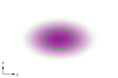
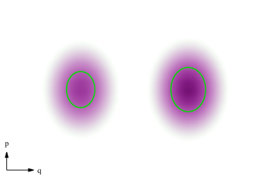
Figure 1: Hamiltonian Monte Carlo generates trajectories that efficiently explore level sets of constant probability, and hence the target distribution itself. (a) The level sets of unimodal target distributions are simply-connected and can be explored with a single trajectory using only local information of the target distribution. (b) On the other hand, the level sets of multimodal target distributions are disconnected, requiring multiple trajectories and global information of the target distribution to ensure comprehensive exploration. Deforming the multimodal target distribution into a unimodal one, however, warps the disconnected level sets into connected ones and dramatically eases sampling.

I Thermodynamic Algorithms

An immediate strategy for deforming a complex distribution into a simpler one is the moderation of the density between the two distributions.

Consider a topological sample space, $Q$, its usual Borel $\sigma$-algebra, $\mathcal{B}\!\left(Q\right)$, and a potentially-complex target distribution, $\pi$. Assuming absolute continuity, we can construct the target distribution from a unimodal and otherwise well-behaved base measure, $\pi_{B}$, and a density incorporating any complicated, possibly multimodal structure,

$$\pi =\frac{\mathrm{d}\pi}{\mathrm{d}\pi_{B}}\pi_{B}$$

$$\equiv e^{-\Delta V}\pi_{B}.$$

We can then generate a continuum of distributions between $\pi_{B}$ and $\pi$ by exponentiating the density,

$$\pi_{\beta} =\frac{1}{Z\!\left(\beta\right)}\left(\frac{\mathrm{d}\pi}{\mathrm{d}\pi_{B}}\right)^{\beta}\pi_{B}$$

$$=\frac{e^{-\beta\,\Delta V}\pi_{B}}{Z\!\left(\beta\right)},$$

where

$$Z\!\left(\beta\right)=\int_{Q}\mathrm{d}\pi_{B}\,e^{-\beta\,\Delta V}.$$

The desired deformation now takes the form of a bijection between any two intermediate distributions,

$$f: \,Q\times\mathbb{R}\rightarrow Q\times\mathbb{R}$$

$$\left(q,\beta\right)\mapsto\left(q^{\prime},\beta^{\prime}\right),$$

which ideally maintains equilibrium,

$$f_{*}\pi_{\beta}=\pi_{\beta^{\prime}}.$$ (1)

Methods traversing this spectrum of distributions are often analogized with thermodynamics, where $\beta$ takes the role of an inverse temperature and $Z\!\left(\beta\right)$ the partition function.

In simulated annealing KirkpatrickEtAl:1983 ; Cerny:1985 ; Neal:1993 a deformation is generated by deterministically pushing $\beta$ along a rigid partition known as a schedule, with the state stochastically evolved in between temperature updates using a Markov chain targeting the current $\pi_{\beta}$. The performance of simulated annealing depends crucially on the sensitivity of $\pi_{\beta}$ to $\beta$ – because the temperature is changed with the state held constant there is no guarantee that the state will remain in equilibrium with respect to the new $\pi_{\beta}$.

Simulated tempering MarinariEtAl:1992 ; Neal:1993 appeals to the same rigid partition but ensures equilibrium by applying a Metropolis correction to each move along the partition. Formally, this generates a Markov chain with transitions proposing the exchange of states at temperatures $\beta$ and $\beta\pm\delta\beta$ with acceptance probability

$$p\!\left(\mathrm{accept}\right)=\min\!\left(1,\frac{\pi_{\beta}\!\left(q_{1}\right)}{\pi_{\beta\pm\delta\beta}\!\left(q_{1}\right)}\frac{\pi_{\beta\pm\delta\beta}\!\left(q_{2}\right)}{\pi_{\beta}\!\left(q_{2}\right)}\right).$$

The cost of maintaining equilibrium is that the random exploration of the temperature partition proceeds only slowly, especially when $\pi_{\beta}$ rapidly varies with $\beta$.

Ultimately both approaches are limited by their dependence on a rigid partition of temperatures. When $\pi_{\beta}$ is highly-sensitive to $\beta$ the probability mass rapidly changes with temperature, frustrating equilibrization in simulated annealing and intensifying random walk behavior in simulated tempering. Formally, the sensitivity can be quantified with the Kullback-Leibler divergence between any neighboring distributions,

$$\mathrm{KL}\!\left(\pi_{\beta}||\pi_{\beta+\delta\beta}\right) =-\int_{Q}\mathrm{d}\pi_{\beta}\log\frac{\mathrm{d}\pi_{\beta+\delta\beta}}{\mathrm{d}\pi_{\beta}}$$

$$=-\int_{Q}\mathrm{d}\pi_{\beta}\log e^{-\delta\beta\,\Delta V}$$

$$\quad-\int_{Q}\mathrm{d}\pi_{\beta}\log\frac{Z\!\left(\beta\right)}{Z\!\left(\beta+\delta\beta\right)}$$

$$=-\delta\beta\int_{Q}\mathrm{d}\pi_{\beta}\left(-\Delta V\right)$$

$$\quad-\log\frac{Z\!\left(\beta\right)}{Z\!\left(\beta+\delta\beta\right)}\int_{Q}\mathrm{d}\pi_{\beta}$$

$$=-\delta\beta\frac{1}{Z\!\left(\beta\right)}\frac{\partial Z}{\partial\beta}\!\left(\beta\right)$$

$$\quad-\log\frac{Z\!\left(\beta\right)}{Z\!\left(\beta+\delta\beta\right)}.$$

Without any dynamic adaptation, the optimal performance of both algorithms is achieved when the deformation is constant across the partition,

$$\mathrm{KL}\!\left(\pi_{\beta}||\pi_{\beta+\delta\beta}\right)\approx\mathrm{const}.$$

Because the partition function is rarely known a priori, however, determining an effective gradation is usually impossible and the algorithms must instead rely on adaptation schemes that themselves are sensitive to the details of the target distribution and its evolution along the partition.

II Adiabatic Monte Carlo

This fragility of simulated annealing and simulated tempering to the temperature schedule arises because proposed moves across the partition do not themselves preserve the intermediate distributions as in (1). Truly measure-preserving processes, however, arise naturally in the thermodynamic analogy as adiabatic processes, which mathematically correspond to special flows on contact manifolds Geiges:2008 ; Lee:2013 . By mapping a given probability space into a contact manifold we can canonically construct these flows, both in theory and in practice, which are capable of exactly mapping samples from $\pi_{B}$ into $\pi$.

II.1 Contact Hamiltonian Flows and Adiabatic Processes

A contact manifold is a $\left(2n+1\right)$-dimensional manifold, $\mathcal{R}$, endowed with a contact form, $\alpha$, satisfying

$$\Omega_{C}=\alpha\wedge\left(\mathrm{d}\alpha\right)^{n}\neq 0;$$

because of this non-degeneracy condition $\Omega_{C}$ serves as a canonical volume form and orients the manifold. A given contact form and a contact Hamiltonian, $H_{C}:\mathcal{R}\rightarrow\mathbb{R}$, uniquely identify a contact vector field by

$$\alpha\!\left(\vec{X}_{H_{C}}\right) =H_{C}$$

$$\left.\mathrm{d}\alpha\!\left(\vec{X}_{H_{C}},\cdot\right)\right|_{\xi} =\left.-\mathrm{d}H_{C}\right|_{\xi},$$

where $\xi$ is the contact structure,

$$\xi=\left\{v\in T\mathcal{R}:\alpha\!\left(v\right)=0\right\}.$$

Locally any contact manifold decomposes into the product of a symplectic manifold and $\mathbb{R}$, yielding the canonical coordinates $\left(q^{i},p_{i},\gamma\right)$. In these canonical coordinates the contact form becomes

$$\alpha=\mathrm{d}\gamma+\theta,$$

where $\theta$ is the local primitive of the symplectic form, $\mathrm{d}\theta=-\Omega$. Any contact vector field then factors into three components,

$$\vec{X}_{H_{C}}= +\left(H_{C}-p_{i}\frac{\partial H_{C}}{\partial p_{i}}\right)\frac{\partial}{\partial\gamma}$$

$$+\left(\frac{\partial H_{C}}{\partial p_{i}}\frac{\partial}{\partial q^{i}}-\frac{\partial H_{C}}{\partial q^{i}}\frac{\partial}{\partial p_{i}}\right)$$

$$+\;\;\,\frac{\partial H_{C}}{\partial\gamma}p_{i}\frac{\partial}{\partial p_{i}}:$$

the first term is a Reeb vector field generating a change in the contact coordinate, $\gamma$; the second term is a symplectic vector field convolving the symplectic coordinates; and the final term is a Liouville vector field that scales the $p$.

Unlike a Hamiltonian flow on a symplectic manifold, a contact Hamiltonian flow does not foliate the contact manifold. In fact the largest integrable submanifolds consistent with a given contact structure,

$$\mathcal{S}\subset\mathcal{R},T\mathcal{S}\subset\xi,$$

are the $n$-dimensional Legendrean submanifolds, and only the flowout of $H_{C}^{-1}\!\left(0\right)$ is constrained to such a submanifold. Thermodynamically, the image of $H_{C}^{-1}\!\left(0\right)$ along a corresponding contact Hamiltonian flow is exactly an adiabatic process Mrugala:1978 .

The statistical utility of adiabatic processes lies in the fact that they preserve both the contact Hamiltonian,

$$\left.\mathcal{L}_{\vec{X}_{H_{C}}}H_{C}\right|_{H_{C}^{-1}\left(0\right)} =\left.\mathrm{d}H\!\left(\vec{X}_{H}\right)\right|_{H_{C}^{-1}\left(0\right)}$$

$$=\left.H_{C}\frac{\partial H_{C}}{\partial\gamma}\right|_{H_{C}^{-1}\left(0\right)}$$

$$=0,$$

and the contact form

$$\left.\mathcal{L}_{\vec{X}_{H}}\alpha\right|_{H_{C}^{-1}\left(0\right)} =\left.\mathcal{L}_{\vec{X}_{H}}\alpha\right|_{\xi}$$

$$=\left.\left(\mathrm{d}\alpha\!\left(\vec{X}_{H},\cdot\right)+\mathrm{d}\left(\alpha\!\left(\vec{X}_{H}\right)\right)\right)\right|_{\xi}$$

$$=\left.\left(\mathrm{d}\alpha\!\left(\vec{X}_{H},\cdot\right)+\mathrm{d}H\right)\right|_{\xi}$$

$$=0.$$

Consequently adiabatic processes also preserve the canonical measure, $\pi_{H_{C}}=e^{-H_{C}}\Omega_{C}$,

$$\left.\mathcal{L}_{\vec{X}_{H_{C}}}\left(\pi_{H_{C}}\right)\right|_{H_{C}^{-1}\left(0\right)}=0,$$

or

$$\left.\left(\phi^{H_{C}}_{t}\right)_{*}\left(\pi_{H_{C}}\right)\right|_{H_{C}^{-1}\left(0\right)}=\pi_{H_{C}}.$$

Recognizing heat in thermodynamics as probability, this measure-preservation corresponds to the property that adiabatic processes exchange no heat with the environment.

One concern with adiabatic processes is that, unlike their symplectic counterparts, contact Hamiltonian flows may have fixed points which prevent the corresponding adiabatic process from being a bijection, and hence preserving the canonical measure, for all $t$.

II.2 Constructing Contact Hamiltonian Systems

For these measure-preserving flows to be the basis of a useful statistical algortihm, we first require a canonical way of manipulating a given probabilistic system into a contact Hamiltonian system. Following the geometric construction of Monte Carlo BetancourtEtAl:2014 , we do this by first mapping the probabilistic system into a Hamiltonian system which we then contactize into a contact Hamiltonian system.

In order to construct a Hamiltonian system we first lift the base measure, $\pi_{B}$, to a measure on the cotangent bundle of the sample space, $\varpi:T^{*}Q\rightarrow Q$, with the choice of a disintegration, $\xi$,

$$\pi_{H}=\varpi^{*}\pi_{B}\wedge\xi=e^{-H}\Omega,$$

where

$$H=-\log\frac{\mathrm{d}\pi_{H}}{\mathrm{d}\Omega}.$$

In canonical coordinates, $\left(q^{i},p_{i}\right)$, we have the decompositions

$$\pi_{B} =e^{-V_{B}}\mathrm{d}^{n}q$$

$$\xi =e^{-T}\mathrm{d}^{n}p+\text{horizontal}\;n\text{-forms},$$

in which case the Hamiltonian becomes

$$H=T+V_{B}.$$

We can now contactize the cotangent bundle by affixing a contact coordinate, $\gamma\in\mathbb{R}$,

$$\mathcal{R}=T^{*}Q\times\mathbb{R},$$

with the corresponding contact form $\alpha=\mathrm{d}\gamma+\theta$, where $\theta$ is the tautological one-form on the cotangent bundle. Finally, we lift $\pi_{H}$ to $\mathcal{R}$ by introducing the density, $\mathrm{d}\pi/\mathrm{d}\pi_{B}$, and some constant, $H_{0}$,

$$\pi_{H_{C}} =\frac{1}{Z\!\left(\beta(\gamma)\right)}\left(\frac{\mathrm{d}\pi}{\mathrm{d}\pi_{B}}\right)^{\beta\left(\gamma\right)}e^{-H_{0}}\alpha\wedge\pi_{H}$$

$$=e^{-H_{C}}\Omega_{C},$$

where $H_{C}$ is the resulting contact Hamiltonian,

$$H_{C}=T+V_{B}+\beta\!\left(\gamma\right)\,\Delta V+\log Z\!\left(\beta(\gamma)\right)+H_{0}.$$

with $Z\!\left(\beta(\gamma)\right)$ the partition function,

$$Z\!\left(\beta(\gamma)\right)=\int_{T^{*}Q}\left.\left(e^{-\left(T+V_{B}+\beta(\gamma)\,\Delta V+H_{0}\right)}\Omega_{C}\right)\right|_{\beta(\gamma)}.$$

In practice $H_{0}$ is chosen to ensure that the initial point lies in the zero level set, $H^{-1}_{C}\!\left(0\right)$.

Now given a particular value of $\gamma$, the distribution $\pi_{H_{C}}$ restricts to a canonical distribution on the cotangent bundle,

$$\pi_{H_{\beta(\gamma)}} =\left.\pi_{H_{C}}\right|_{\beta(\gamma)}$$

$$=e^{-\left.H_{C}\right|_{\beta(\gamma)}}\Omega$$

$$\equiv e^{H_{\beta(\gamma)}}\Omega,$$

which then projects down to a distribution on the target sample space,

$$\pi_{\beta(\gamma)} =\varpi^{*}\pi_{H_{\beta(\gamma)}}$$

$$=\frac{1}{Z\!\left(\beta(\gamma)\right)}\left(\frac{\mathrm{d}\pi}{\mathrm{d}\pi_{B}}\right)^{\beta\left(\gamma\right)}\pi_{B}.$$

In order to map $\gamma\in\mathbb{R}$ into the interval $\beta\in\left[0,1\right]$, I will assume the relationship

$$\beta\!\left(\gamma\right)=\frac{1}{1+e^{-\gamma}}$$ (2)

through the rest of the paper.

Adiabatic processes are then generated by contact Hamiltonian flowout of $H_{C}^{-1}\!\left(0\right)$,

$$\left.\vec{X}_{H_{C}}\right|_{H_{C}^{-1}(0)}= -p_{i}\frac{\partial H_{C}}{\partial p_{i}}\frac{\partial}{\partial\gamma}$$

$$+\left(\frac{\partial H_{C}}{\partial p_{i}}\frac{\partial}{\partial q^{i}}-\frac{\partial H_{C}}{\partial q^{i}}\frac{\partial}{\partial p_{i}}\right)$$

$$+\left(\Delta V-\mathbb{E}_{\pi_{H_{\beta}}}\!\left[\Delta V\right]\right)\beta\left(1-\beta\right)p_{i}\frac{\partial}{\partial p_{i}}.$$

Because the contact Hamiltonian flow preserves the lift of the target distribution by construction, it features all of the properties we were lacking in simulated annealing and simulated tempering.

The Reeb component generates dynamic updates to the temperature, avoiding the need for a pre-defined partition. These updates are coherent and avoid the random exploration that can limit simulated tempering – for example, when the disintegration is constructed from a Riemannian metric, $g$, GirolamiEtAl:2011 ; BetancourtEtAl:2014 ,

$$T\!\left(q,p\right) =A\cdot F\!\left(g^{-1}\!\left(p,p\right)\right)$$

$$\quad+\frac{1}{2}\log\left|g\!\left(q\right)\right|+\mathrm{const},$$ (3)

the updates are monotonic.

Between temperature updates, the symplectic and Liouville components maintain the equilibrium that simulated annealing lacks. The Liouville component of the flow can also be thought of as a perfect thermostat, in comparison to the approximate thermostats, such as the Nosé–Hoover thermostat EvansEtAl:1985 , common to molecular dynamics.

In other words, adiabatic processes gives us the directed temperature exploration of simulated annealing, the equilibrium maintenance of simulated tempering, and a dynamic temperature partition that neither enjoy (Figure 2).

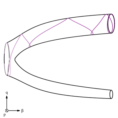
Figure 2: Contact Hamiltonian flow generates trajectories that move through a continuum of Hamiltonian systems between the Hamiltonian system corresponding to the simple base distribution at $\beta=0$ and the Hamiltonian system corresponding to the potentially complex target distribution at $\beta=1$. The trajectories corresponding to adiabatic processes dynamically adapt to maintain equilibrium at each temperature.

An additional benefit of adiabatic processes is immediate recovery of the partition function $Z\!\left(\beta\right)$ at any time along the flow. Because the contact Hamiltonian vanishes on the zero level set, the partition function is given at any point by

$$-\log Z\!\left(\beta\right)=T+V_{B}+\beta\,\Delta V+H_{0},$$ (4)

provided that the densities are all properly normalized. Unlike most thermodynamic integration methods GelmanEtAl:1998 , this is an instantaneous result and does not require any quadrature.

Unfortunately, the contact Hamiltonian systems produced in this construction are not immune to fixed points. For example, if we take a Riemannian disintegration (3) then fixed points arise when the target parameters settle into a minimum of the effective potential energy, $V_{B}+\beta\,\Delta V$, the momenta fall to zero, and the flow along $\gamma$ stops (Figure 3). These fixed points correspond to metastable states in thermodynamics; cooling metastabilities are accessed by flowing from $\beta=0$ to $\beta=1$ while heating metastabilities are accessed by flowing from $\beta=1$ to $\beta=0$ (Figure 4).

Metastable states obstruct the flow from being an bijection between $\beta=0$ and $\beta=1$. For example, consider a cooling transition from $\beta=0$ to $\beta=1$, or, recalling (2), $\gamma=-\infty$ to $\gamma=\infty$. Cooling metastabilities restrict the preimage of the flow and obstruct its surjectivity, while heating metastabilities restrict the image of the flow and obstruct its injectivity.

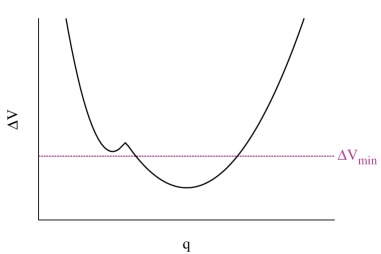
Figure 3: Metastable equilibria occur when the Liousville component of the contact Hamiltonian flow forces the momenta to zero too rapidly. Consequently the flow relaxes into a local minimum such as $\Delta V_{\mathrm{min}}$ and the temperature ceases to update.

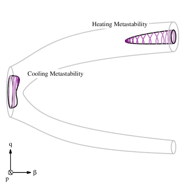
Figure 4: A potential pathology of contact Hamiltonian flow are fixed points, or metastable states. Cooling metastabilities arise when a trajectory originating from $\beta=0$ stalls, while heating metastabilities arise when a trajectory originating from $\beta=1$ stalls. When a contact Hamiltonian flow suffers from metastabilities it is not an bijection between the two temperatures and samples from one distribution are not necessarily mapped to samples from the other.

II.3 Implementing Adiabatic Monte Carlo

Once a disintegration has been chosen, in theory Adiabatic Monte Carlo proceeds similar to Hamiltonian Monte Carlo. A sample from the base distribution,

$$q_{i}\sim\pi,$$

is first lifted to the cotangent bundle by sampling from the local fiber,

$$q_{i}\mapsto z_{i}=(q_{i},p_{i}),\,p_{i}\sim\iota_{q_{i}}^{*}\xi,$$

and then to the contact manifold by setting $\beta=0$. The constant $H_{0}$ is chosen such that the initial point falls on $H_{C}^{-1}\!\left(0\right)$ and the system is evolved backwards in time until $\beta=1$ via a cooling transition,

$$\left(z_{f},\beta=1\right)=\phi^{H_{C}}_{-t}\!\left(z_{i},\beta=0\right),$$

and then projected back down to the sample space,

$$q_{f}=\varpi\!\left(z_{f}\right).$$

Implementing this algorithm in practice, however, is significantly more complicated. In addition to simulating the contact Hamiltonian flow, which requires not only an accurate numeral integrator but also the accurate estimation of intermediate expectations and possibly temperature-dependent adaptation, we must also overcome possible fixed points in the contact Hamiltonian flow.

II.3.1 Simulating Contact Hamiltonian Flow

Typically the contact Hamiltonian flow will not be solvable in practice and we must instead rely on a numerical approximation. Fortunately, contact Hamiltonian flow admits an accurate and robust numerical approximation in the same way that symplectic integrators approximate Hamiltonian flow.

Following the geometric construction of a symplectic integrator HairerEtAl:2006 , we can approximate the contact Hamiltonian flow by first splitting the contact Hamiltonian into three scalar functions,

$$H_{C} =\underbrace{T}_{H_{1}}+\underbrace{V_{B}}_{H_{2}}+\underbrace{\beta\Delta V+\log Z\!\left(\beta\right)}_{H_{3}}+H_{0}.$$

This gives three vector fields along the contact structure,

$$\vec{X}_{H_{1}} =\frac{\partial T}{\partial p_{i}}\left(\frac{\partial}{\partial q^{i}}-p_{i}\frac{\partial}{\partial\beta}\right)-\frac{\partial T}{\partial q^{i}}\frac{\partial}{\partial p_{i}}$$

$$\vec{X}_{H_{2}} =-\frac{\partial V_{B}}{\partial q^{i}}\frac{\partial}{\partial p_{i}}$$

$$\vec{X}_{H_{3}} =\left[-\beta\frac{\partial\Delta V}{\partial q^{i}}+\left(\Delta V-\mathbb{E}_{\pi_{H_{\beta}}}\!\left[\Delta V\right]\right)p_{i}\right]\frac{\partial}{\partial p_{i}},$$

and three corresponding contact Hamiltonian flows, $\phi_{t}^{H_{1}}$, $\phi_{t}^{H_{2}}$, and $\phi_{t}^{H_{3}}$. If the intermediate expectations $\mathbb{E}_{\pi_{H_{\beta}}}\!\left[\Delta V\right]$ are known then each of these flows can be solved immediately and their symmetric composition gives a reversible, second-order approximation to the exact flow (Algo II.3.1),

$$\phi_{\tau}^{H_{C}} =\left(\phi_{\epsilon/2}^{H_{1}}\circ\phi_{\epsilon/2}^{H_{2}}\circ\phi_{\epsilon}^{H_{3}}\circ\phi_{\epsilon/2}^{H_{2}}\circ\phi_{\epsilon/2}^{H_{1}}\right)^{\tau/\epsilon}$$

$$\quad+\mathcal{O}\!\left(\epsilon^{2}\right).$$

Because each component is a contact Hamiltonian flow, their composition is also a contact Hamiltonian flow. Consequently the numerical integration exactly preserves the contact volume form with only a small error in the contact Hamiltonian itself that can be controlled by manipulating the integrator step size, $\epsilon$.

Assuming that the expectations $\mathbb{E}_{\pi_{H_{\beta}}}\!\left[\Delta V\right]$ are known, a second-order and reversible contact integrator is readily constructed by simulating flows from component contact Hamiltonians.

Initialize $\beta=0$, $q\sim\pi_{\beta}$, $p\sim\iota^{*}_{q}\xi$

$H_{0}\leftarrow-\left(T\!\left(q,p\right)+V\!\left(q\right)\right)$

while  $\beta<1$  do

   $\beta\leftarrow\beta-\left(-\epsilon/2\right)p\cdot\partial T/\partial p$ $\phi^{H_{1}}_{-\epsilon/2}$

   $q\leftarrow q+\left(-\epsilon/2\right)\quad\,\,\partial T/\partial p$

   

   $p\leftarrow p-\left(-\epsilon/2\right)\partial V_{B}/\partial q$ $\phi^{H_{2}}_{-\epsilon/2}$

   $p\leftarrow p-\left(-\epsilon\right)\beta\,\partial\Delta V/\partial q$ $\phi^{H_{3}}_{-\epsilon}\;\,$

   $\quad\quad\quad\;\;+\left(-\epsilon\right)\left(\Delta V-\mathbb{E}_{\pi_{H_{\beta}}}\!\left[\Delta V\right]\right)p$

   

   $p\leftarrow p-\left(-\epsilon/2\right)\partial V_{B}/\partial q$ $\phi^{H_{2}}_{-\epsilon/2}$

   $\beta\leftarrow\beta-\left(-\epsilon/2\right)p\cdot\partial T/\partial p$ $\phi^{H_{1}}_{-\epsilon/2}$

   $q\leftarrow q+\left(-\epsilon/2\right)\quad\,\,\partial T/\partial p$

end while

Proper normalization of $\Delta V$ required

$-\log Z\!\left(\beta\right)=T\!\left(q,p\right)+V\!\left(q\right)+\beta\Delta V\!\left(q\right)+H_{0}$

In order to exactly compensate for the error in the approximate integration of the contact Hamiltonian flow we can appeal to the same Metropolis acceptance procedure often used in Hamiltonian Monte Carlo, although with some slight modifications. If there are no metastabilties, for example, then a proposal targeting $\pi_{H_{\beta=1}}$ can be constructed by composing a heating transition with a momentum resampling and finally a cooling transition. Given an initial state, $\left(q_{i},p_{i}\right)$, the final state $\left(q_{f},p_{f}\right)$ can then be accepted with probability

$$p\!\left(\mathrm{accept}\right) =$$

$$\min\!\left[1,\exp\!\left(H_{\beta=1}\!\left(p_{i},q_{i}\right)-H_{\beta=1}\!\left(p_{f},q_{f}\right)\right)\right].$$

Care must be taken with such a Metropolis correction, however, when the contact Hamiltonian flow is subject to metastabilities and hence is not a proper bijection.

II.3.2 Estimating Expectations

Of course in any practical problem the expectations $\mathbb{E}_{\pi_{H_{\beta}}}\!\left[\Delta V\right]$ will not be known a priori and we must instead estimate them online. An immediate strategy is to use Hamiltonian Monte Carlo initialized at the current state, which should already be in local equilibrium.

Running Hamiltonian Monte Carlo at each step of the contact integrator can quickly become computationally limiting, and ensuring exact reversibility of the resulting contact trajectories is a delicate problem. A more robust approach is to run an ensemble of initial trajectories that estimate the expectations at each step. These intermediate expectations can be smoothed with a nonparametric estimator, such as a Gaussian process, and then used to implement accurate, fast, and exactly reversible trajectories.

When targeting multimodal distributions we have to be more careful still as each initial trajectory will be able to estimate the expectations with respect to only the local mode. In order to construct an accurate global expectation we have to weight the local expectations by the local partition functions, which are conveniently provided by the contact Hamiltonian flow at no additional cost.

Finally, if we want to use the partition function then we must consider how the error in any such estimation scheme propagates to deviations in the contact Hamiltonian.

II.3.3 Adapting to Temperature-Dependent Curvature

One of the powerful features of Hamiltonian Monte Carlo is that the disintegration can be tuned to optimize the performance of a symplectic integrator in a certain coordinate system.

For example, Euclidean Hamiltonian Monte Carlo utilizes a Gaussian disintegration given by

$$T=\frac{1}{2}M^{-1}\!\left(p,p\right)+\frac{1}{2}\log\left|M\right|;$$ (5)

when the inverse Euclidean Metric, $M^{-1}$, is aligned with the global covariance of the coordinates, symplectic integrators can be run with larger step sizes, lower costs, and fewer pathologies. Similarly, Riemannian Hamiltonian Monte Carlo utilizes a position-dependent metric aligned with the local covariance of the target distribution.

Tuning the kinetic energy in Adiabatic Monte Carlo is more subtle given that the curvature of $\pi_{\beta}$ can vary sharply with $\beta$. In practice this may require a temperature-dependent disintegration and a resultantly more complicated contact Hamiltonian flow. One of the advantages of a Riemannian Hamiltonian Monte Carlo with the SoftAbs metric Betancourt:2013b is that an optimal temperature-dependent tuning is given implicitly by the metric itself.

II.3.4 Overcoming Metastabilities

As noted above, the contact Hamiltonian flow may exhibit fixed points which manifest as metastable states obstructing and obstruct the flow from being a bijection.

Fortunately both cooling and heating metastabilities can be overcome by simply resampling the momentum often enough – resampling near a cooling metastability kicks the flow out of the local minimum ensuring subjectivity while resampling after a heating metastability allows the flow to access all final states and recovers injectivity. Moreover, if $H_{0}$ is incremented with the difference in kinetic energies before and after the resampling,

$$H_{0}\rightarrow H_{0}+T_{\mathrm{before}}-T_{\mathrm{after}},$$

then the partition function can still be recovered from (4).

The implementation challenge is in exactly when to interrupt the contact Hamiltonian flow with a momentum resampling. Because the temperature evolution slows as the flow approaches a cooling metastability, resampling the momentum at uniform time intervals is sufficient to avoid the metastability itself. Recovering from heating metastabilities, however, is more challenging because the metastability has no immediate impact on the flow. Instead we can only assume the presence of heating metastabilities and resample often as the flow approaches $\beta=1$. Additionally, if we want to apply a Metropolis correction then any resampling scheme must also be reversible.

III Beta-Binomial Example

In order to demonstrate the power of adiabatic processes without concerning ourselves with metstabilties, let us a examine a simple one-dimensional and univariate example. In particular, consider the Beta distribution taking the role of both the target and base distributions with a Binomial density between them,

$$\pi_{\beta} \propto\left(\mathrm{Bi}\!\left(k|n\right)\right)^{\beta}\mathrm{Be}\!\left(a,b\right)$$

$$=\mathrm{Be}\!\left(\beta\,k+a,\beta\left(n-k\right)+b\right).$$

In this case we can analytically compute both the partition function,

$$Z\!\left(\beta\right) =\left[\frac{\Gamma\!\left(n+1\right)}{\Gamma\!\left(k+1\right)\Gamma\!\left(n-k+1\right)}\right]^{\beta}\frac{\Gamma\!\left(a+b\right)}{\Gamma\!\left(a\right)\Gamma\!\left(b\right)}$$

$$=\quad\times\frac{\Gamma\!\left(\beta\,k+a\right)\Gamma\!\left(\beta\left(n-k\right)+b\right)}{\Gamma\!\left(\beta\,n+a+b\right)},$$

and its derivative,

$$\frac{1}{Z\!\left(\beta\right)}\frac{\partial Z\!\left(\beta\right)}{\partial\beta} =\;\;\,\log\!\left(\frac{\Gamma\!\left(n+1\right)}{\Gamma\!\left(k+1\right)\Gamma\!\left(n-k+1\right)}\right)$$

$$\quad+k\,\psi\!\left(\beta\,k+a\right)$$

$$\quad+\left(n-k\right)\psi\!\left(\beta\left(n-k\right)+b\right)$$

$$\quad-n\,\psi\!\left(\beta\,n+a+b\right).$$

In the following I take $a=9$, $b=0.75$, $k=115$, and $n=550$ such that the target and base distributions have only small overlap (Figure 5, 5) and a rapidly changing partition function (Figure 5).

Given these analytic results we can readily investigate the performance of simulated annealing, simulated tempering, and then Adiabatic Monte Carlo. Note that with the preponderance of analytic results in this example, both simulated annealing and simulated tempering can be tuned to achieve reasonable performance. Our goal here is not to demonstrate that the existing algorithms fail in this simple case but rather to exemplify the kinds of pathologies that become unavoidable when targeting complex distributions in high dimensions.

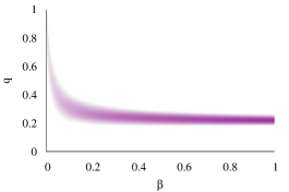
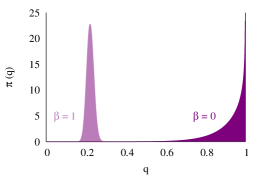
Figure 5: Emulative of the difficult models encountered in practice, the target and base distributions in the experiments have little overlap which exposes the weakness of simulated annealing and simulated tempering. Here (a, b) the probability mass rapidly slides from one boundary towards the other as the inverse temperature, $\beta$ increases from 0 to 1. Consequently, (c) the partition function is also extremely sensitive to the inverse temperature.

III.1 Simulated Annealing

Here I implemented simulated annealing with two Random Walk Metropolis RobertEtAl:1999 transitions in between temperature updates. At each temperature I tuned the proposal scale to achieve the optimal acceptance probability for a one-dimensional target distribution RobertsEtAl:1997 .

I ran simulated annealing three times, each with a different partition of the inverse temperature: a coarse partition consisting of 25 evenly spaced intervals, a fine partition consisting of 100 evenly spaced intervals, and an optimally-tuned partition consisting of 25 intervals such that the Kullback-Leibler divergence between each partition is constant.

The coarse partition is not well-tuned to the local variations in $\pi_{\beta}$; the state rapidly falls out of equilibrium and then converges only well after the target distribution stops changing with temperature (Figure 6). Only with much smaller (Figure 6) and optimally-tuned (Figure 6) partitions does the state remain in equilibrium throughout the entire transition.

The biggest weakness of simulated annealing is not so much that the state can fall out of equilibrium but rather that falling out of equilibrium can be extremely difficult to diagnose in practice. As the target distribution becomes more complex, especially as it grows in dimensionality, the potential for falling out of equilibrium and not re-converging becomes greater and greater. Consequently, simulated annealing is not a particularly robust choice for statistical applications.

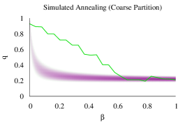
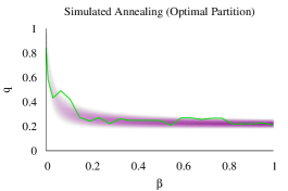
Figure 6: Even for this one-dimensional target distribution simulated annealing can (a) rapidly fall out of equilibrium for coarse partitions. Only with (b) very fine and (c) optimally-tuned partitions can equilibrium be maintained.

III.2 Simulated Tempering

As above, I implemented simulated tempering three times, using Random Walk Metropolis optimally tuned to the coarse, fine, and tuned partitions. After 25 warmup transitions at $\beta=0$ the chain evolves by jumping between neighboring temperatures in the partition.

In all three cases simulated tempering is able to maintain equilibrium as expected. When using the coarse (Figure 7) and fine (Figure 7) partitions, however, the active state explores inefficiently never reaches $\beta=1$. Only with the tuned partition can information propagate between $\beta=0$ and $\beta=1$ in a reasonable amount of time (Figure 7).

More complex transitions between temperatures offer some hope of improving the inefficient exploration but in practice they are difficult to tune, especially when considering the high dimensional target distributions of interest.

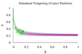
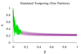
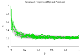
Figure 7: Although simulated tempering maintains the equilibrium that simulated annealing is prone to losing, the efficacy of its temperature exploration depends critically on the configuration of the partition. Both (a) the course partition and (b) the fine partition suffer from amplified random walk behavior. (c) Only the tuned partition admits reasonably efficient exploration.

III.3 Adiabatic Monte Carlo

I implemented Adiabatic Monte Carlo with the Gaussian Euclidean disintegration (5) and the resulting integrator as described in Algorithm II.3.1. The expectation $\mathbb{E}_{\pi_{H_{\beta}}}\!\left[\Delta V\right]$ was estimated at each temperature using Hamiltonian Monte Carlo seeded at the current position of the chain. For both the contact Hamiltonian flow and the intermediate Hamiltonian Monte Carlo runs the step size was set to $\epsilon=0.01$, and the integration time for Hamiltonian Monte Carlo was randomly sampled as $\tau\sim U\left[0,2\varpi\right)$.

Without requiring any temperature partition, Adiabatic Monte Carlo is able to maintain equilibrium while efficiently exploring all temperatures by effectively determining a partition dynamically (Figure 8). As desired, the temperature changes dynamically slow as the trajectory deviates away from equilibrium and increases only once the trajectory has returned to the bulk of the probability mass (Figure 8). Moreover, without any additional computation the trajectory also provides an accurate estimate of the partition function (Figure 9).

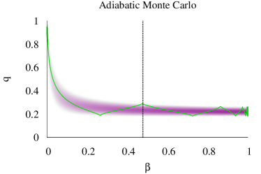
Figure 8: (a) Adiabatic Monte Carlo utilizes a contact Hamiltonian flow to transition between temperatures while maintaining equilibrium. (b) Because the temperature is a dynamic component of the flow, the evolution effectively determines an optimal temperature partition dynamically. As the trajectory moves away from the probability mass, for example at the dotted line, the temperature evolution slows to give the trajectory time to return to equilibrium.

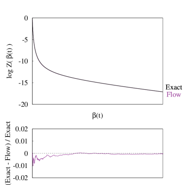
Figure 9: A convenient byproduct of contact Hamiltonian flow is an accurate estimate of the partition function at each inverse temperature, $\beta$. The error in the estimate is too small to be seen in the upper panel even as the true partition function varies across 8 orders of magnitude.

IV Conclusion

By leveraging the geometry of contact Hamiltonian systems, Adiabatic Monte Carlo admits a uniquely powerful approach to exploring the complex and multimodal target distributions that confound Markov Chain Monte Carlo algorithms. Moreover, this foundational geometry not only identifies potential pathologies, such as metastabilities, but also guides the construction of the implementations robust to those pathologies. Algorithms incorporating this guidance are currently under development with the ultimate goal an implementation in Stan Stan:2014 .

V Acknowledgements

I thank Tarun Chitra, Andrew Gelman, Mark Girolami, Matt Johnson, and Stephan Mandt for thoughtful comments and Chris Wendl for illuminating contact geometries. This work was supported by EPSRC grant EP/J016934/1.

References

- (1) C. P. Robert and G. Casella, Monte Carlo Statistical Methods (Springer New York, 1999).
- (2) S. Brooks, A. Gelman, G. L. Jones, and X.-L. Meng, editors, Handbook of Markov Chain Monte Carlo (CRC Press, New York, 2011).
- (3) S. Duane, A. Kennedy, B. J. Pendleton, and D. Roweth, Physics Letters B 195, 216 (1987).
- (4) R. Neal, MCMC using Hamiltonian dynamics, in Handbook of Markov Chain Monte Carlo, edited by S. Brooks, A. Gelman, G. L. Jones, and X.-L. Meng, CRC Press, New York, 2011.
- (5) M. Betancourt, S. Byrne, S. Livingstone, and M. Girolami, ArXiv e-prints 1410.5110 (2014).
- (6) S. Kirkpatrick et al., Science 220, 671 (1983).
- (7) V. Černøy, Journal of Optimization Theory and Applications 45, 41 (1985).
- (8) R. Neal, Department of Computer Science, University of Toronto Report No. CRG-TR-93-1, 1993 (unpublished).
- (9) E. Marinari and G. Parisi, Europhysics Letters 19, 451 (1992).
- (10) H. Geiges, An Introduction to Contact Topology (Cambridge Univ. Press, 2008).
- (11) J. M. Lee, Introduction to Smooth Manifolds (Springer, 2013).
- (12) R. Mrugała, Reports on Mathematical Physics 14, 419 (1978).
- (13) M. Girolami and B. Calderhead, Journal of the Royal Statistical Society: Series B (Statistical Methodology) 73, 123 (2011).
- (14) D. J. Evans and B. L. Holian, The Journal of Chemical Physics 83, 4069 (1985).
- (15) A. Gelman and X.-L. Meng, Statistical science , 163 (1998).
- (16) E. Hairer, C. Lubich, and G. Wanner, Geometric Numerical Integration: Structure-Preserving Algorithms for Ordinary Differential Equations (Springer, New York, 2006).
- (17) M. Betancourt, A general metric for Riemannian Hamiltonian Monte Carlo, in First International Conference on the Geometric Science of Information, edited by F. Nielsen and F. Barbaresco, , Lecture Notes in Computer Science Vol. 8085, Springer, 2013.
- (18) G. O. Roberts et al., The annals of applied probability 7, 110 (1997).
- (19) Stan Development Team, Stan: A C++ library for probability and sampling, version 2.5, 2014.