Numerical approximation of phase field based shape and topology optimization for fluids

Abstract

We consider the problem of finding optimal shapes of fluid domains. The fluid obeys the Navier–Stokes equations. Inside a holdall container we use a phase field approach using diffuse interfaces to describe the domain of free flow. We formulate a corresponding optimization problem where flow outside the fluid domain is penalized. The resulting formulation of the shape optimization problem is shown to be well-posed, hence there exists a minimizer, and first order optimality conditions are derived.

For the numerical realization we introduce a mass conserving gradient flow and obtain a Cahn–Hilliard type system, which is integrated numerically using the finite element method. An adaptive concept using reliable, residual based error estimation is exploited for the resolution of the spatial mesh.

The overall concept is numerically investigated and comparison values are provided.

Key words. Shape optimization, topology optimization, diffuse interfaces, Cahn–Hilliard, Navier–Stokes, adaptive meshing.

AMS subject classification. 35Q35, 35Q56, 35R35, 49Q10, 65M12, 65M22, 65M60, 76S05.

1 Introduction

Shape and topology optimization in fluid mechanics is an important mathematical field attracting more and more attention in recent years. One reason therefore is certainly the wide application fields spanning from optimization of transport vehicles like airplanes and cars, over biomechanical and industrial production processes to the optimization of music instruments. Due to the complexity of the emerging problems those questions have to be treated carefully with regard to modelling, simulation and interpretation of the results. Most approaches towards shape optimization, in particular in the field of shape optimization in fluid mechanics, deal mainly with numerical methods, or concentrate on combining reliable CFD methods to shape optimization strategies like the use of shape sensitivity analysis. Anyhow, it is a well-known fact that well-posedness of problems in optimal shape design is a difficult matter where only a few analytical results are available so far, see for instance [9, 10, 30, 34, 39, 40]. In particular, classical formulations of shape optimization problems lack in general existence of a minimizer and hence the correct mathematical description has to be reconsidered. Among first approaches towards well-posed formulations in this field we mention in particular the work [6], where a porous medium approach is introduced in order to obtain a well-posed problem at least for the special case of minimizing the total potential power in a Stokes flow. As discussed in [17, 18] it is not to be expected that this formulation can be extended without further ado to the stationary Navier–Stokes equations or to the use of different objective functionals.

In this work we propose a well-posed formulation for shape optimization in fluids, which will turn out to even allow for topological changes. Therefore, we combine the porous medium approach of [6] and a phase field approach including a regularization by the Ginzburg-Landau energy. This results in a diffuse interface problem, which can be shown to approximate a sharp interface problem for shape optimization in fluids that is penalized by a perimeter term. Perimeter penalization in shape optimization problems was already introduced by [2] and has since then been applied to a lot of problems in shape optimization, see for instance [8]. Also phase field approximations for the perimeter penalized problems have been discussed in this field, and we refer here for instance to [5, 8, 11]. But to the best of our knowledge, neither a perimeter penalization nor a phase field approach has been applied to a fluid dynamical setting before.

Here we use the stationary incompressible Navier–Stokes equations as a fluid model, but we briefly describe how the Stokes equations could also be used here. The resulting diffuse interface problem is shown to inherit a minimizer, in contrast to most formulations in shape optimization. The resulting formulation turns out to be an optimal control problem with control in the coefficients, and hence one can derive optimality conditions in form of a variational inequality. Thus, we can formulate a gradient flow for the corresponding reduced objective functional and arrive in a Cahn–Hilliard type system. Similar to [29], we use a Moreau–Yosida relaxation in order to handle the pointwise constraints on the design variable. We formulate the finite element discretization of the resulting problem using a splitting approach for the Cahn–Hilliard equation. The Navier–Stokes system is discretized with the help of Taylor–Hood elements and both variables in the Cahn–Hilliard equation are discretized with continuous, piecewise linear elements. In addition, we introduce an adaptive concept using residual based error estimates and a Dörfler marking strategy, see also [28, 29].

The proposed approach is validated by means of several numerical examples. The first one shows in particular that even topological changes are allowed during the optimization process. The second example is the classical example of optimizing the shape of a ball in an outer flow. We obtain comparable results as in the literature and discuss the results for different Reynolds numbers and penalization parameters. For this example, comparison values for further investigations are provided. As a third example and outlook, we briefly discuss the optimal embouchure of a bassoon, which was already examined by an engineering group at the Technical University of Dresden, see [25]. Besides, the behaviour of the different parameters of the model and their influence on the obtained solution in the above-mentioned numerical examples are investigated.

2 Shape and topology optimization for Navier–Stokes flow

We study the optimization of some objective functional depending on the shape, geometry and topology of a region which is filled with an incompressible Navier–Stokes fluid. We use a holdall container $\Omega\subset\mathbb{R}^{d}$ which is fixed throughout this work and fulfills

• $\Omega\subseteq\mathbb{R}^{d}$, $d\in\{2,3\}$, is a bounded Lipschitz domain with outer unit normal $\boldsymbol{n}$ such that $\mathbb{R}^{d}\setminus\overline{\Omega}$ is connected.

Requiring the complement of $\overline{\Omega}$ to be connected simplifies certain aspects in the analysis of the Navier–Stokes system but could also be dropped, cf. [27, Remark 2.7]. As we do not want to prescribe the topology or geometric properties of the optimal fluid region in advance, we state the optimization problem in the general framework of Caccioppoli sets. Thus, a set is admissible if it is a measurable subset of $\Omega$ with finite perimeter. Additionally, we impose a volume constraint by introducing a constant $\beta\in\left(-1,1\right)$ and optimize over the sets with volume equal to $0.5(\beta+1)\left|\Omega\right|$. Since an optimization problem in this setting lacks in general existence of minimizers, see for instance [3], we introduce moreover a perimeter regularization. Thus the perimeter term, multiplied by some weighting parameter $\gamma>0$ and a constant $c_{0}=\frac{\pi}{2}$ arising due to technical reasons, is added to the objective functional that we want to minimize. The latter is given by $\int_{\Omega}f\left(x,\boldsymbol{u},\mathrm{D}\boldsymbol{u}\right)\,\mathrm{d}x$, where $\boldsymbol{u}\in\boldsymbol{U}:=\{\boldsymbol{u}\in\boldsymbol{H}^{1}(\Omega)\mid\,\mathrm{div}\,\boldsymbol{u}=0,\boldsymbol{u}|_{\partial\Omega}=\boldsymbol{g}\}$ denotes the velocity of the fluid, and we assume

• the functional $f:\Omega\times\mathbb{R}^{d}\times\mathbb{R}^{d\times d}\to\mathbb{R}$ is given such that

  $$F:\boldsymbol{H}^{1}(\Omega)\to\mathbb{R},$$

  $$F\left(\boldsymbol{u}\right):=\int_{\Omega}f\left(x,\boldsymbol{u}(x),\mathrm{D}\boldsymbol{u}(x)\right)\,\mathrm{d}x$$

  is continuous, weakly lower semicontinuous, radially unbounded in $\boldsymbol{U}$, which means

  $$\lim_{k\to\infty}\left\|\boldsymbol{u}_{k}\right\|_{\boldsymbol{H}^{1}(\Omega)}=+\infty\implies\lim_{k\to\infty}F\left(\boldsymbol{u}_{k}\right)=+\infty$$ (1)

  for any sequence $\left(\boldsymbol{u}_{k}\right)_{k\in\mathbb{N}}\subseteq\boldsymbol{U}$. Additionally, $F|_{\boldsymbol{U}}$ has to be bounded from below.

Here and in the following we use the following function space:

$$\boldsymbol{V}:=\left\{\boldsymbol{v}\in\boldsymbol{H}^{1}_{0}(\Omega)\mid\,\mathrm{div}\,\boldsymbol{u}=0\right\}.$$

Additionally, we denote for some $\varphi\in BV\left(\Omega,\left\{\pm 1\right\}\right)$ the set $E^{\varphi}:=\{\varphi\equiv 1\}$ and introduce

$$\boldsymbol{U}^{\varphi}:=\left\{\boldsymbol{u}\in\boldsymbol{U}\mid\boldsymbol{u}=\boldsymbol{0}\text{ a.e. in }\Omega\setminus E^{\varphi}\right\},\quad\boldsymbol{V}^{\varphi}:=\left\{\boldsymbol{v}\in\boldsymbol{V}\mid\boldsymbol{v}=\boldsymbol{0}\text{ a.e. in }\Omega\setminus E^{\varphi}\right\},$$

where we remark, that we denote $\mathbb{R}^{d}$-valued functions and function spaces of vector valued functions by boldface letters.

Remark 1.

For the continuity of $F:\boldsymbol{H}^{1}(\Omega)\to\mathbb{R}$, required in Assumption (A2), it is sufficient, that $f:\Omega\times\mathbb{R}^{d}\times\mathbb{R}^{d\times d}\to\mathbb{R}$ is a Carathéodory function, i.e. $f$ fulfills for a.e. $x\in\Omega$ a growth condition of the form

$$\left|f\left(x,\boldsymbol{v},\boldsymbol{A}\right)\right|\leq a(x)+b_{1}(x)|\boldsymbol{v}|^{p}+b_{2}(x)|\boldsymbol{A}|^{2},\quad\forall\boldsymbol{v}\in\mathbb{R}^{d},\boldsymbol{A}\in\mathbb{R}^{d\times d}$$

for some $a\in L^{1}(\Omega)$, $b_{1},b_{2}\in L^{\infty}(\Omega)$ and some $p\geq 2$ for $d=2$ and $2\leq p\leq\nicefrac{{2d}}{{d-2}}$ for $d=3$.

For the fluid mechanics, we use Dirichlet boundary conditions on $\partial\Omega$, thus there may be some inflow or some outflow, and we allow additionally external body forces on the whole domain $\Omega$.

• Here, $\boldsymbol{f}\in\boldsymbol{L}^{2}(\Omega)$ is the applied body force and $\boldsymbol{g}\in\boldsymbol{H}^{\frac{1}{2}}\left(\partial\Omega\right)$ is some given boundary function such that $\int_{\partial\Omega}\boldsymbol{g}\cdot\boldsymbol{n}\,\mathrm{d}s=0$,

which are assumed to be given and fixed throughout this paper.

A typical objective functional used in this context is the total potential power, which is given by

$$f\left(x,\boldsymbol{u},\mathrm{D}\boldsymbol{u}\right):=\frac{\mu}{2}\left|\mathrm{D}\boldsymbol{u}\right|^{2}-\boldsymbol{f}(x)\cdot\boldsymbol{u}.$$ (2)

In particular, we remark that this functional fulfills Assumption (A2).

To formulate the problem, we introduce an one-to-one correspondence of Caccioppoli sets and functions of finite perimeter by identifying $E\subset\Omega$ with $\varphi:=2\chi_{E}-1\in BV\left(\Omega,\left\{\pm 1\right\}\right)$ and notice that for any $\varphi\in BV\left(\Omega,\left\{\pm 1\right\}\right)$ the set $E^{\varphi}:=\left\{\varphi=1\right\}$ is the corresponding Caccioppoli set describing the fluid region. We shall write $P_{\Omega}(E)$ for the perimeter of $E\subseteq\Omega$ in $\Omega$. For a more detailed introduction to the theory of Caccioppoli sets and functions of bounded variations we refer for instance to [16, 24].

Altogether we arrive in the following optimization problem:

$$\min_{\left(\varphi,\boldsymbol{u}\right)}J_{0}\left(\varphi,\boldsymbol{u}\right):=\int_{\Omega}f\left(x,\boldsymbol{u},\mathrm{D}\boldsymbol{u}\right)\,\mathrm{d}x+\gamma c_{0}P_{\Omega}\left(E^{\varphi}\right)$$ (3)

subject to

$$\varphi\in\Phi_{ad}^{0}:=\left\{\varphi\in BV\left(\Omega,\left\{\pm 1\right\}\right)\mid\int_{\Omega}\varphi\,\mathrm{d}x=\beta\left|\Omega\right|,\boldsymbol{U}^{\varphi}\neq\emptyset\right\}$$

and

$$-\mu\Delta\boldsymbol{u}+\left(\boldsymbol{u}\cdot\nabla\right)\boldsymbol{u}+\nabla p =\boldsymbol{f} \text{in }E^{\varphi},$$ (4a)

$$-\,\mathrm{div}\,\boldsymbol{u} =0 \text{in }\Omega,$$ (4b)

$$\boldsymbol{u} =\boldsymbol{0} \text{in }\Omega\setminus E^{\varphi},$$ (4c)

$$\boldsymbol{u} =\boldsymbol{g} \text{on }\partial\Omega.$$ (4d)

We point out that the velocity of the fluid is not only defined on the fluid region $E^{\varphi}$, for some $\varphi\in\Phi_{ad}^{0}$, but rather on the whole of $\Omega$, where in $E^{\varphi}$ it is determined by the stationary Navier-Stokes equations, and on the remainder we set it equal to zero. And so for an arbitrary function $\varphi\in BV(\Omega,\left\{\pm 1\right\})$ the condition $\boldsymbol{u}=\boldsymbol{0}$ a.e. in $\Omega\setminus E^{\varphi}$ and the non-homogeneous boundary data $\boldsymbol{u}=\boldsymbol{g}$ on $\partial\Omega$ may be inconsistent. To exclude this case we impose the condition $\boldsymbol{U}^{\varphi}\neq\emptyset$ on the admissible design functions in $\Phi_{ad}^{0}$. The state constraints (4) have to be fulfilled in the following weak sense: find $\boldsymbol{u}\in\boldsymbol{U}^{\varphi}$ such that it holds

$$\int_{\Omega}\mu\nabla\boldsymbol{u}\cdot\nabla\boldsymbol{v}+\left(\boldsymbol{u}\cdot\nabla\right)\boldsymbol{u}\cdot\boldsymbol{v}\,\mathrm{d}x=\int_{\Omega}\boldsymbol{f}\cdot\boldsymbol{v}\,\mathrm{d}x\quad\forall\boldsymbol{v}\in\boldsymbol{V}^{\varphi}.$$

Even though this shape and topology optimization problem gives rise to a large class of possible solutions, numerics and analysis prefer more regularity for handling optimization problems. One common approach towards more analytic problem formulations is a phase field formulation. It is a well-known fact, see for instance [33], that a multiple of the perimeter functional is the $L^{1}(\Omega)$-$\Gamma$-limit for $\varepsilon\searrow 0$ of the Ginzburg-Landau energy, which is defined by

$$\mathcal{E}_{\varepsilon}\left(\varphi\right):=\begin{cases}\int_{\Omega}\frac{\varepsilon}{2}\left|\nabla\varphi\right|^{2}+\frac{1}{\varepsilon}\psi\left(\varphi\right)\,\mathrm{d}x,&\text{if }\varphi\in H^{1}(\Omega),\\ +\infty,&\text{otherwise.}\end{cases}$$

Here $\psi:\mathbb{R}\to\overline{\mathbb{R}}$ is a potential with two global minima and in this work we focus on a double obstacle potential given by

$$\psi(\varphi):=\begin{cases}\psi_{0}\left(\varphi\right),&\text{if }\left|\varphi\right|\leq 1,\\ +\infty,&\text{otherwise,}\end{cases}\quad\psi_{0}\left(\varphi\right):=\frac{1}{2}\left(1-\varphi^{2}\right).$$

Thus replacing the perimeter functional by the Ginzburg-Landau energy in the objective functional, we arrive in a so-called diffuse interface approximation, where the hypersurface between fluid and non-fluid region is replaced by a interfacial layer with thickness proportional to some small parameter $\varepsilon>0$. Then the design variable $\varphi$ is allowed to have values in $\left[-1,1\right]$ instead of only $\pm 1$. To make sense of the state equations in this setting, we introduce an interpolation function $\alpha_{\varepsilon}:\left[-1,1\right]\to\left[0,\overline{\alpha}_{\varepsilon}\right]$ fulfilling the following assumptions:

• Let $\alpha_{\varepsilon}:\left[-1,1\right]\to\left[0,\overline{\alpha}_{\varepsilon}\right]$ be a decreasing, surjective and twice continuously differentiable function for $\varepsilon>0$.

  It is required that $\overline{\alpha}_{\varepsilon}>0$ is chosen such that $\lim_{\varepsilon\searrow 0}\overline{\alpha}_{\varepsilon}=+\infty$ and $\alpha_{\varepsilon}$ converges pointwise to some function $\alpha_{0}:[-1,1]\to[0,+\infty]$. Additionally, we impose $\alpha_{\delta}(x)\geq\alpha_{\varepsilon}(x)$ if $\delta\leq\varepsilon$ for all $x\in\left[-1,1\right]$, $\lim_{\varepsilon\searrow 0}\alpha_{\varepsilon}(0)<\infty$ and a growth condition of the form $\overline{\alpha}_{\varepsilon}=\hbox{o}\left(\varepsilon^{-\frac{2}{3}}\right)$.

Remark 2.

We remark, that for space dimension $d=2$ we can even choose $\overline{\alpha}_{\varepsilon}=\hbox{o}\left(\varepsilon^{-\kappa}\right)$ for any $\kappa\in(0,1)$.

By adding the term $\alpha_{\varepsilon}(\varphi)\boldsymbol{u}$ to (4a) we find that the state equations (4) then “interpolate” between the steady-state Navier–Stokes equations in $\left\{\varphi=1\right\}$ and some Darcy flow through porous medium with permeability $\overline{\alpha}_{\varepsilon}^{-1}$ at $\left\{\varphi=-1\right\}$. Thus simultaneously to introducing a diffuse interface approximation, we weaken the condition of non-permeability through the non-fluid region. This porous medium approach has been introduced for topology optimization in fluid flow by [6]. To ensure that the velocity vanishes outside the fluid region in the limit $\varepsilon\searrow 0$ we add moreover a penalization term to the objective functional and finally arrive in the following phase field formulation of the problem:

$$\begin{split}\min_{\left(\varphi,\boldsymbol{u}\right)}J_{\varepsilon}\left(\varphi,\boldsymbol{u}\right)&:=\int_{\Omega}\frac{1}{2}\alpha_{\varepsilon}\left(\varphi\right)\left|\boldsymbol{u}\right|^{2}\,\mathrm{d}x+\int_{\Omega}f\left(x,\boldsymbol{u},\mathrm{D}\boldsymbol{u}\right)\,\mathrm{d}x\\ &+\frac{\gamma\varepsilon}{2}\int_{\Omega}\left|\nabla\varphi\right|^{2}\,\mathrm{d}x+\frac{\gamma}{\varepsilon}\int_{\Omega}\psi\left(\varphi\right)\,\mathrm{d}x\end{split}$$ (5)

subject to

$$\varphi\in\Phi_{ad}:=\left\{\varphi\in H^{1}(\Omega)\mid\left|\varphi\right|\leq 1\text{ a.e. in }\Omega,\int_{\Omega}\varphi\,\mathrm{d}x=\beta\left|\Omega\right|\right\},$$ (6)

and

$$\alpha_{\varepsilon}(\varphi)\boldsymbol{u}-\mu\Delta\boldsymbol{u}+\left(\boldsymbol{u}\cdot\nabla\right)\boldsymbol{u}+\nabla p =\boldsymbol{f} \text{in }\Omega,$$ (7a)

$$-\,\mathrm{div}\,\boldsymbol{u} =0 \text{in }\Omega,$$ (7b)

$$\boldsymbol{u} =\boldsymbol{g} \text{on }\partial\Omega.$$ (7c)

Considering the state equations (7), we find the following solvability result:

Lemma 1.

For every $\varphi\in L^{1}(\Omega)$ such that $\left|\varphi\right|\leq 1$ a.e. in $\Omega$ there exists some $\boldsymbol{u}\in\boldsymbol{U}$ such that (7) is fulfilled in the following sense:

$$\int_{\Omega}\alpha_{\varepsilon}\left(\varphi\right)\boldsymbol{u}\cdot\boldsymbol{v}+\mu\nabla\boldsymbol{u}\cdot\nabla\boldsymbol{v}+\left(\boldsymbol{u}\cdot\nabla\right)\boldsymbol{u}\cdot\boldsymbol{v}\,\mathrm{d}x=\int_{\Omega}\boldsymbol{f}\cdot\boldsymbol{v}\,\mathrm{d}x\quad\forall\boldsymbol{v}\in\boldsymbol{V}.$$ (8)

Besides, if there exists a solution $\boldsymbol{u}\in\boldsymbol{U}$ of (8) such that it holds

$$\left\|\nabla\boldsymbol{u}\right\|_{\boldsymbol{L}^{2}(\Omega)}<\frac{\mu}{K_{\Omega}},\quad K_{\Omega}:=\begin{cases}\nicefrac{{2}}{{3}}\sqrt{2}|\Omega|^{\frac{2}{3}},&\text{if }d=3,\\ 0.5\sqrt{\left|\Omega\right|},&\text{if }d=2,\end{cases}$$ (9)

then this is the only solution of (8).

Proof.

The existence proof is based on the theory on pseudo-monotone operators and the uniqueness statement follows similar to classical results concerning stationary Navier–Stokes equations, see for instance [20, 27]. ∎

Remark 3.

Standard results infer from (8) that there exists a pressure $p\in L^{2}(\Omega)$ associated to $\boldsymbol{u}\in\boldsymbol{U}$ such that (7) is fulfilled in a weak sense, see [20]. But as we are not considering the pressure dependency in the optimization problem, we drop those considerations in the following. For details on how to include the pressure in the objective functional in this setting we refer to [27].

Using this result, one can show well-posedness of the optimal control problem in the phase field formulation stated above by exploiting the direct method in the calculus of variations.

Theorem 2.

There exists at least one minimizer $(\varphi_{\varepsilon},\boldsymbol{u}_{\varepsilon})$ of (5)–(7).

The proof is given in [27].

To derive first order necessary optimality conditions for a solution $(\varphi_{\varepsilon},\boldsymbol{u}_{\varepsilon})$ of (5)–(7) we introduce the Lagrangian $\mathcal{L}_{\varepsilon}:\Phi_{ad}\times\boldsymbol{U}\times\boldsymbol{V}\to\mathbb{R}$ by

$$\mathcal{L}_{\varepsilon}\left(\varphi,\boldsymbol{u},\boldsymbol{q}\right):=J_{\varepsilon}(\varphi,\boldsymbol{u})-\int_{\Omega}\alpha_{\varepsilon}\left(\varphi\right)\boldsymbol{u}\cdot\boldsymbol{q}+\mu\nabla\boldsymbol{u}\cdot\nabla\boldsymbol{q}+\left(\boldsymbol{u}\cdot\nabla\right)\boldsymbol{u}\cdot\boldsymbol{q}-\boldsymbol{f}\cdot\boldsymbol{q}\,\mathrm{d}x.$$

The variational inequality is formally derived by

$$\begin{split}\mathrm{D}_{\varphi}\mathcal{L}_{\varepsilon}\left(\varphi_{\varepsilon},\boldsymbol{u}_{\varepsilon},\boldsymbol{q}_{\varepsilon}\right)\left(\varphi-\varphi_{\varepsilon}\right),\geq 0\quad\forall\varphi\in\Phi_{ad}\end{split}$$ (10)

and the adjoint equation can be deduced by

$$\mathrm{D}_{\boldsymbol{u}}\mathcal{L}_{\varepsilon}\left(\varphi_{\varepsilon},\boldsymbol{u}_{\varepsilon},\boldsymbol{q}_{\varepsilon}\right)\left(\boldsymbol{v}\right)=0\quad\forall\boldsymbol{v}\in\boldsymbol{V}.$$

Even though those calculations are only formally, we obtain therefrom a first order optimality system, which can be proved to be fulfilled for a minimizer of the optimal control problem stated above, see [27]:

Theorem 3.

Assume $\left(\varphi_{\varepsilon},\boldsymbol{u}_{\varepsilon}\right)\in\Phi_{ad}\times\boldsymbol{U}$ is a minimizer of (5)–(7) such that $\left\|\nabla\boldsymbol{u}_{\varepsilon}\right\|_{\boldsymbol{L}^{2}(\Omega)}<\nicefrac{{\mu}}{{K_{\Omega}}}$. Then the following variational inequality is fulfilled:

$$\begin{split}\left(\frac{1}{2}\alpha^{\prime}_{\varepsilon}\left(\varphi_{\varepsilon}\right)\left|\boldsymbol{u}_{\varepsilon}\right|^{2}+\frac{\gamma}{\varepsilon}\psi^{\prime}_{0}\left(\varphi_{\varepsilon}\right)-\alpha^{\prime}_{\varepsilon}\left(\varphi_{\varepsilon}\right)\boldsymbol{u}_{\varepsilon}\cdot\boldsymbol{q}_{\varepsilon}+\lambda_{\varepsilon},\varphi-\varphi_{\varepsilon}\right)_{L^{2}(\Omega)}\\ +\left(\gamma\varepsilon\nabla\varphi_{\varepsilon},\nabla\left(\varphi-\varphi_{\varepsilon}\right)\right)_{\boldsymbol{L}^{2}(\Omega)}\geq 0\quad\forall\varphi\in\overline{\Phi}_{ad},\end{split}$$ (11)

with

$$\overline{\Phi}_{ad}:=\left\{\varphi\in H^{1}(\Omega)\mid\left|\varphi\right|\leq 1\,\text{ a.e. in }\Omega\right\},$$

where $\boldsymbol{q}_{\varepsilon}\in\boldsymbol{V}$ is the unique weak solution to the following adjoint system:

$$\alpha_{\varepsilon}\left(\varphi_{\varepsilon}\right)\boldsymbol{q}_{\varepsilon}-\mu\Delta\boldsymbol{q}_{\varepsilon}+\left(\nabla\boldsymbol{u}_{\varepsilon}\right)^{T}\boldsymbol{q}_{\varepsilon}-\left(\boldsymbol{u}_{\varepsilon}\cdot\nabla\right)\boldsymbol{q}_{\varepsilon}+\nabla\pi_{\varepsilon} =\alpha_{\varepsilon}\left(\varphi_{\varepsilon}\right)\boldsymbol{u}_{\varepsilon}$$

$$+\mathrm{D}_{2}f\left(\cdot,\boldsymbol{u}_{\varepsilon},\mathrm{D}\boldsymbol{u}_{\varepsilon}\right)-\,\mathrm{div}\,\mathrm{D}_{3}f\left(\cdot,\boldsymbol{u}_{\varepsilon},\mathrm{D}\boldsymbol{u}_{\varepsilon}\right) \text{in }\Omega,$$ (12a)

$$-\,\mathrm{div}\,\boldsymbol{q}_{\varepsilon} =0 \text{in }\Omega,$$ (12b)

$$\boldsymbol{q}_{\varepsilon} =\boldsymbol{0} \text{on }\partial\Omega.$$ (12c)

Here, we denote by $\mathrm{D}_{i}f\left(\cdot,\boldsymbol{u}_{\varepsilon},\mathrm{D}\boldsymbol{u}_{\varepsilon}\right)$ with $i=2$ and $i=3$ the differential of $f:\Omega\times\mathbb{R}^{d}\times\mathbb{R}^{d\times d}$ with respect to the second and third component, respectively. Besides, $\boldsymbol{u}_{\varepsilon}$ solves the state equations $\eqref{e:StatNSStrong}$ corresponding to $\varphi_{\varepsilon}$ in the weak sense and $\lambda_{\varepsilon}\in\mathbb{R}$ is a Lagrange multiplier for the integral constraint. Additionally, $\pi_{\varepsilon}\in L^{2}(\Omega)$ can as in Remark 3 be obtained as pressure associated to the adjoint system.

Under certain assumptions on the objective functional it can be verified that a minimizer $(\varphi_{\varepsilon},\boldsymbol{u}_{\varepsilon})$ of (5)–(7) fulfills $\left\|\nabla\boldsymbol{u}_{\varepsilon}\right\|_{\boldsymbol{L}^{2}(\Omega)}<\nicefrac{{\mu}}{{K_{\Omega}}}$. This implies by Lemma 1 that $\boldsymbol{u}_{\varepsilon}$ is the only solution of (7) corresponding to $\varphi_{\varepsilon}$, see [27]. In particular, for minimizing the total potential power, see (2), this condition is equivalent to stating “smallness of data or high viscosity” as can be found in classical literature. For details and the proof of Theorem 3 we refer the reader to [27].

Hence it is not too restrictive to assume from now on that in a neighborhood of the minimizer $\varphi_{\varepsilon}$ the state equations (7) are uniquely solvable, such that we can introduce the reduced cost functional $j_{\varepsilon}(\varphi):=J_{\varepsilon}(\varphi,\boldsymbol{u})$ where $\boldsymbol{u}$ is the solution to (7) corresponding to $\varphi$. The optimization problem (5)–(7) is then equivalent to $\min_{\varphi\in\Phi_{ad}}j_{\varepsilon}(\varphi)$.

Following [29], we consider a Moreau–Yosida relaxation of this optimization problem

$$\min_{\varphi\in\Phi_{ad}}j_{\varepsilon}(\varphi) \hat{P}_{\infty}$$ ()

in which the primitive constraints $|\varphi|\leq 1$ $a.e.$ in $\Omega$ are replaced (relaxed) through an additional quadratic penalization term in the cost functional. The optimization problem then reads

$$\min_{\varphi\in H^{1}(\Omega),\int_{\Omega}\varphi\,\mathrm{d}x=\beta|\Omega|}j_{\varepsilon}^{s}(\varphi), \hat{P}_{s}$$ ()

where

$$j_{\varepsilon}^{s}(\varphi):=j_{\varepsilon}(\varphi)+\frac{s}{2}\int_{\Omega}\left|\max\left(0,\varphi-1\right)\right|^{2}\,\mathrm{d}x+\frac{s}{2}\int_{\Omega}\left|\min\left(0,\varphi+1\right)\right|^{2}\,\mathrm{d}x.$$ (13)

Here, $s\gg 1$ plays the role of the penalization parameter. The associated Lagrangian $\mathcal{L}_{\varepsilon}^{s}$ reads then correspondingly

$$\begin{split}\mathcal{L}_{\varepsilon}^{s}\left(\varphi,\boldsymbol{u},\boldsymbol{q}\right)&:=J_{\varepsilon}(\varphi,\boldsymbol{u})+\frac{s}{2}\int_{\Omega}\left|\max\left(0,\varphi-1\right)\right|^{2}\,\mathrm{d}x+\frac{s}{2}\int_{\Omega}\left|\min\left(0,\varphi+1\right)\right|^{2}\,\mathrm{d}x\\ &-\int_{\Omega}\alpha_{\varepsilon}\left(\varphi\right)\boldsymbol{u}\cdot\boldsymbol{q}+\mu\nabla\boldsymbol{u}\cdot\nabla\boldsymbol{q}+\left(\boldsymbol{u}\cdot\nabla\right)\boldsymbol{u}\cdot\boldsymbol{q}-\boldsymbol{f}\cdot\boldsymbol{q}\,\mathrm{d}x.\end{split}$$ (14)

Similar analysis as above yields the gradient equation

$$\begin{split}&\mathrm{D}_{\varphi}\mathcal{L}_{\varepsilon}^{s}\left(\varphi_{\varepsilon},\boldsymbol{u}_{\varepsilon},\boldsymbol{q}_{\varepsilon}\right)\varphi=\left(\frac{1}{2}\alpha^{\prime}_{\varepsilon}\left(\varphi_{\varepsilon}\right)\left|\boldsymbol{u}_{\varepsilon}\right|^{2}+\frac{\gamma}{\varepsilon}\psi^{\prime}_{0}\left(\varphi_{\varepsilon}\right)-\alpha^{\prime}_{\varepsilon}\left(\varphi_{\varepsilon}\right)\boldsymbol{u}_{\varepsilon}\cdot\boldsymbol{q}_{\varepsilon}+\lambda_{s}(\varphi_{\varepsilon}),\varphi\right)_{L^{2}(\Omega)}\\ &+\left(\gamma\varepsilon\nabla\varphi_{\varepsilon},\nabla\varphi\right)_{\boldsymbol{L}^{2}(\Omega)}=0,\end{split}$$ (15)

which has to hold for all $\varphi\in H^{1}(\Omega)$ with $\int_{\Omega}\varphi\,\mathrm{d}x=0$. Here we use $\lambda_{s}(\varphi_{\varepsilon})=\lambda_{s}^{+}(\varphi_{\varepsilon})+\lambda_{s}^{-}(\varphi_{\varepsilon})$ with $\lambda_{s}^{+}(\varphi_{\varepsilon}):=s\max\left(0,\varphi_{\varepsilon}-1\right)$ and $\lambda_{s}^{-}(\varphi_{\varepsilon}):=s\min\left(0,\varphi_{\varepsilon}+1\right)$, and $\boldsymbol{q}_{\varepsilon}\in\boldsymbol{V}$ is the adjoint state given as weak solution of (12). The functions $\lambda_{s}^{+}(\varphi_{\varepsilon})$ and $\lambda_{s}^{-}(\varphi_{\varepsilon})$ can also be interpreted as approximations of Lagrange multipliers for the pointwise constraints $\varphi\leq 1$ a.e. in $\Omega$ and $\varphi\geq-1$ a.e. in $\Omega$, respectively.

It can be shown, that the sequence of minimizers $\left(\varphi_{\varepsilon},\boldsymbol{u}_{\varepsilon}\right)_{\varepsilon>0}$ of (5)–(7) has a subsequence that converges in $L^{1}(\Omega)\times\boldsymbol{H}^{1}(\Omega)$ as $\varepsilon\searrow 0$. If the sequence $\left(\varphi_{\varepsilon}\right)_{\varepsilon>0}$ converges of order $\mathcal{O}\left(\varepsilon\right)$ one obtains that the limit element actually is a minimizer of (3)–(4). In these particular cases, one can additionally prove that the first order optimality conditions given by Theorem 3 are an approximation of the classical shape derivatives for the shape optimization problem (3)–(4). For details we refer the reader to [27].

Remark 4.

The same analysis and considerations can be carried out in a Stokes flow. For the typical example of minimizing the total potential power (2) it can then even be shown, that the reduced objective functional corresponding to the phase field formulation $\Gamma$-converges in $L^{1}(\Omega)$ to the reduced objective functional of the sharp interface formulation. Moreover, the first order optimality conditions are much simpler since no adjoint system is necessary any more. For details we refer to [27].

3 Numerical solution techniques

To solve the phase field problem (5)–(7) numerically, we use a steepest descent approach. For this purpose, we assume as above that in a neighborhood of the minimizer $\varphi_{\varepsilon}$ the state equations (7) are uniquely solvable, and hence the reduced cost functional $j_{\varepsilon}(\varphi):=J_{\varepsilon}(\varphi,\boldsymbol{u})$, with $\boldsymbol{u}$ the solution to (7) corresponding to $\varphi$, is well-defined. In addition, we introduce an artificial time variable $t$. Our aim consists in finding a stationary point in $\Phi_{ad}$ of the following gradient flow:

$$\left\langle\partial_{t}\varphi,\zeta\right\rangle=-\mathrm{grad}j_{\varepsilon}^{s}(\varphi)(\zeta)=-\mathrm{D}j_{\varepsilon}^{s}(\varphi)(\zeta)\quad\forall\zeta\in H^{1}(\Omega),\int_{\Omega}\zeta\,\mathrm{d}x=0,$$ (16)

with some inner product $\left\langle\cdot,\cdot\right\rangle$, where $j_{\varepsilon}^{s}$ is the Moreau–Yosida relaxed cost functional defined in (13). This flow then decreases the cost functional $j_{\varepsilon}^{s}$.
Now a stationary point $\varphi_{\varepsilon}\in\Phi_{ad}$ of this flow fulfills the necessary optimality condition (15). Obviously, the resulting equation depends on the choice of the inner product. Here, we choose an $H^{-1}$-inner product which is defined as

$$\left(v_{1},v_{2}\right)_{H^{-1}(\Omega)}:=\int_{\Omega}\nabla\left(-\Delta\right)^{-1}v_{1}\cdot\nabla\left(-\Delta\right)^{-1}v_{2}\,\mathrm{d}x,$$

where $y=(-\Delta)^{-1}v$ for $v\in\left(H^{1}(\Omega)\right)^{\star}$ with $\left<v,1\right>=0$ is the weak solution of $-\Delta y=v$ in $\Omega$, $\partial_{\nu}y=0$ on $\partial\Omega$. The gradient flow (16) with this particular choice of $\left\langle\cdot,\cdot\right\rangle=\left(\cdot,\cdot\right)_{H^{-1}(\Omega)}$ reads as follows:

$$\partial_{t}\varphi =\Delta w \quad\text{in }\Omega,$$

$$\left(-w,\xi\right)_{L^{2}(\Omega)} =-\mathrm{D}j_{\varepsilon}^{s}(\varphi)(\xi) \quad\forall\xi\in H^{1}(\Omega),\int_{\Omega}\xi\,\mathrm{d}x=0,$$

together with homogeneous Neumann boundary conditions on $\partial\Omega$ for $\varphi$ and $w$. The resulting problem can be considered as a generalised Cahn–Hilliard system. It follows from direct calculations that this flow preserves the mass, i.e. $\int_{\Omega}\varphi(t,x)\,\mathrm{d}x=\int_{\Omega}\varphi(0,x)\,\mathrm{d}x$ for all $t$. In particular, no Lagrange multiplier for the integral constraint is needed any more. After fixing some initial condition $\varphi_{0}\in H^{1}(\Omega)$ such that $\left|\varphi_{0}\right|\leq 1$ a.e. and $\int_{\Omega}\varphi_{0}\,\mathrm{d}x=\beta\left|\Omega\right|$, and some final time $T>0$ this results in the following problem:

Cahn–Hilliard System:

Find sufficiently regular $\left(\varphi,w,\boldsymbol{u}\right)$ such that

$$\partial_{t}\varphi =\Delta w \text{in }\Omega\times(0,T),$$ (17a)

$$-\gamma\varepsilon\Delta\varphi+\lambda_{s}(\varphi)+\frac{\gamma}{\varepsilon}\psi^{\prime}_{0}(\varphi)+\alpha^{\prime}_{\varepsilon}(\varphi)\left(\frac{1}{2}\left|\boldsymbol{u}\right|^{2}-\boldsymbol{u}\cdot\boldsymbol{q}\right) =w \text{in }\Omega\times(0,T),$$ (17b)

$$\varphi(0) =\varphi_{0} \text{in }\Omega,$$ (17c)

$$\partial_{\nu}\varphi=0,\,\partial_{\nu}w =0 \text{on }\partial\Omega\times\left(0,T\right),$$ (17d)

where $\boldsymbol{u}(t)$ fulfills the state equations (7) corresponding to $\varphi(t)$, and $\boldsymbol{q}(t)$ is the adjoint variable defined by (12).

3.1 Numerical implementation

For a numerical realization of the gradient flow method for finding (locally) optimal topologies we discretize the systems (7), (12) and (17) in time and space.

For this let $0=t_{0}<t_{1}<\ldots<t_{k}<t_{k+1}<\ldots$ denote a time grid with step sizes $\tau_{k}=t_{k}-t_{k-1}$. For ease of presentation we use a fixed step size and thus set $\tau_{k}\equiv\tau$, but we note, that in our numerical implementation $\tau$ is adapted to the gradient flow in direction $\nabla w$, see Section 4.1.

Next a discretization in space using the finite element method is performed. For this let $\mathcal{T}^{k}$ denote a conforming triangulation of $\Omega$ with closed simplices $T\subset\overline{\Omega}$. For simplicity we assume that $\overline{\Omega}$ is exactly represented by $\mathcal{T}^{k}$, i.e. $\overline{\Omega}=\bigcup_{T\in\mathcal{T}^{k}}T$. The set of faces of $\mathcal{T}^{k}$ we denote by $\mathcal{E}^{k}$, while the set of nodes we denote by $\mathcal{N}^{k}$. For each simplex $T\in\mathcal{T}^{k}$ we denote its diameter by $h_{T}$, and for each face $E\in\mathcal{E}^{k}$ its diameter by $h_{E}$. We introduce the finite element spaces

$$\mathcal{V}^{1}(\mathcal{T}^{k}) =\{v\in C(\overline{\Omega})\,|\,v|_{T}\in P_{1}(T),\,\forall T\in\mathcal{T}^{k}\},$$

$$\boldsymbol{\mathcal{V}}^{2}_{\boldsymbol{g}_{h}}(\mathcal{T}^{k}) =\{v\in C(\overline{\Omega})^{d}\,|\,v|_{T}\in P_{2}(T)^{d},\,\forall T\in\mathcal{T}^{k},\,v|_{\partial\Omega}=\boldsymbol{g}_{h}\},$$

where $P_{k}(T)$ denotes the set of all polynomials up to order $k$ defined on the triangle $T$. The boundary data $\boldsymbol{v}|_{\partial\Omega}=\boldsymbol{g}$ is incorporated by a suitable approximation $\boldsymbol{g}_{h}$ of $\boldsymbol{g}$ on the finite element mesh.

Now at time instance $t_{k}$ we by $\boldsymbol{u}_{h}\in\boldsymbol{\mathcal{V}}^{2}_{\boldsymbol{g}_{h}}(\mathcal{T}^{k+1})$ denote the fully discrete variant of $\boldsymbol{u}$ and by $\boldsymbol{q}_{h}\in\boldsymbol{\mathcal{V}}^{2}_{0}(\mathcal{T}^{k+1})$ the fully discrete variant of $\boldsymbol{q}$. Accordingly we proceed with the discrete variants $\varphi_{h},w_{h},p_{h},\pi_{h}\in\mathcal{V}^{1}(\mathcal{T}^{k})$ of $\varphi,w,p$, and $\pi$, where $\int_{\Omega}p_{h}\,\mathrm{d}x=\int_{\Omega}\pi_{h}\,\mathrm{d}x=0$ is required.

Let $\boldsymbol{q}^{k}$ and $\varphi^{k}$ denote the adjoint velocity and the phase field variable from the time step $t_{k}$, respectively. At time instance $t_{k+1}$ we consider

$$\alpha_{\varepsilon}(\varphi^{k})\boldsymbol{u}_{h}-\mu\Delta\boldsymbol{u}_{h}+\left(\boldsymbol{u}_{h}\cdot\nabla\right)\boldsymbol{u}_{h}+\nabla p_{h} =\boldsymbol{f},$$ (18a)

$$\,\mathrm{div}\,\boldsymbol{u}_{h} =0,$$ (18b)

$$\alpha_{\varepsilon}(\varphi^{k})\boldsymbol{q}_{h}-\mu\Delta\boldsymbol{q}_{h}-\left(\boldsymbol{u}_{h}\cdot\nabla\right)\boldsymbol{q}_{h}+\nabla\pi_{h} =\alpha_{\varepsilon}(\varphi^{k})\boldsymbol{u}_{h}+\mathrm{D}_{2}f(\cdot,\boldsymbol{u}_{h},\mathrm{D}\boldsymbol{u}_{h})$$ (19a)

$$-\,\mathrm{div}\,\mathrm{D}_{3}f\left(\cdot,\boldsymbol{u}_{h},\mathrm{D}\boldsymbol{u}_{h}\right)-\left(\nabla\boldsymbol{u}_{h}\right)^{T}\boldsymbol{q}^{k},$$ (19b)

$$\,\mathrm{div}\,\boldsymbol{q}_{h} =0,$$ (19c)

$$\tau^{-1}(\varphi_{h}-\varphi^{k})-\Delta w_{h} =0,$$ (20a)

$$-\gamma\varepsilon\Delta\varphi_{h}+\lambda_{s}(\varphi_{h})+\frac{\gamma}{\varepsilon}\psi_{0}^{\prime}(\varphi^{k})+\alpha_{\varepsilon}^{\prime}(\varphi_{h})\left(\frac{1}{2}|\boldsymbol{u}_{h}|^{2}-\boldsymbol{u}_{h}\cdot\boldsymbol{q}_{h}\right) =w_{h},$$ (20b)

as discrete counterpart to (7), (12) and (17), respectively.

The weak form of (20) using $\psi_{0}^{\prime}(\varphi^{k})=-\varphi^{k}$ reads

$$F^{1}((\varphi_{h},w_{h}),v) =\tau^{-1}(\varphi_{h}-\varphi^{k},v)_{L^{2}(\Omega)}+\left(\nabla w_{h},\nabla v\right)_{\boldsymbol{L}^{2}(\Omega)}=0, \forall v\in\mathcal{V}^{1}(\mathcal{T}^{k+1}),$$ (21a)

$$F^{2}((\varphi_{h},w_{h}),v) =\gamma\varepsilon(\nabla\varphi_{h},\nabla v)_{\boldsymbol{L}^{2}(\Omega)}+(\lambda_{s}(\varphi_{h}),v)_{L^{2}(\Omega)}-\frac{\gamma}{\varepsilon}(\varphi^{k},v)_{L^{2}(\Omega)}$$

$$+\left(\alpha_{\varepsilon}^{\prime}(\varphi_{h})\left(\frac{1}{2}|\boldsymbol{u}_{h}|^{2}-\boldsymbol{u}_{h}\cdot\boldsymbol{q}_{h}\right),v\right)_{L^{2}(\Omega)}-(w_{h},v)_{L^{2}(\Omega)}=0, \forall v\in\mathcal{V}^{1}(\mathcal{T}^{k+1}).$$ (21b)

The time discretization is chosen to obtain a sequential coupling of the three equations of interest. Namely to obtain the phase field on time instance $t_{k+1}$ we first solve (18) for $\boldsymbol{u}_{h}$ using the phase field $\varphi^{k}$ from the previous time step. With $\boldsymbol{u}_{h}$ and $\varphi^{k}$ at hand we then solve (19) to obtain the adjoint velocity $\boldsymbol{q}_{h}$ which then together with $\boldsymbol{u}_{h}$ is used to obtain a new phase field $\varphi^{k+1}$ from (20).

Remark 5.

It follows from the structure of (18)–(20), that $\varphi_{h}$ and $\boldsymbol{u}_{h},\boldsymbol{q}_{h}$ could be discretized on different spatial grids. In the numerical part we for simplicity use one grid for all variables involved.

To justify the discretization (18)–(20) we state the following assumptions.

• The interpolation function $\alpha_{\varepsilon}:[-1,1]\to[0,\overline{\alpha_{\varepsilon}}]$ is extended to $\tilde{\alpha}_{\varepsilon}:\mathbb{R}\to\mathbb{R}$ fulfilling Assumption (A4), so that there exists $0\leq\delta<\infty$ such that $\tilde{\alpha}_{\varepsilon}(\varphi)\geq-\delta$ for all $\varphi\in\mathbb{R}$, with $\delta$ sufficiently small. For convenience we in the following do not distinguish $\alpha_{\varepsilon}$ and $\tilde{\alpha}_{\varepsilon}$.

• For given $\varphi^{k}\in\mathcal{V}^{1}(\mathcal{T}^{k})$ let $\boldsymbol{u}_{h}$ denote the solution to (18) and $\boldsymbol{q}_{h}$ denote the corresponding solution to (19). Then there holds

  $$\frac{1}{2}|\boldsymbol{u}_{h}|^{2}-\boldsymbol{u}_{h}\cdot\boldsymbol{q}_{h}\geq 0.$$

• Additional to Assumption (A4), we assume that $\alpha_{\varepsilon}$ is convex.

Remark 6.

Assumption (A5) is required to ensure existence of unique solutions to (18) and (19) if $\delta$ is sufficiently small.

Assumption (A6) is fulfilled in our numerics for small Reynolds numbers but can not be justified analytically. This assumption might be neglected if $\alpha_{\varepsilon}^{\prime}$ is discretized explicitly in time in (20b). Due to the large values that $\alpha_{\varepsilon}^{\prime}$ takes, we expect a less robust behaviour of the numerical solution process if we discretize $\alpha_{\varepsilon}^{\prime}$ explicitly in time.

Using Assumption (A5) and Assumption (A6) the existence of a unique solution to (20) follows from [29].

For a general $\alpha_{\varepsilon}$ one can use a splitting $\alpha_{\varepsilon}=\alpha_{\varepsilon}^{+}+\alpha_{\varepsilon}^{-}$ where $\alpha_{\varepsilon}^{+}$ denotes the convex part of $\alpha_{\varepsilon}$ and $\alpha_{\varepsilon}^{-}$ denotes the concave part. Then $\alpha_{\varepsilon}^{+}$ is discretized implicitly in time as in (20b), and $\alpha_{\varepsilon}^{-}$ is discretized explicitly in time to obtain a stable discretization, see e.g. [19, 21].

The system (18) is solved by an Oseen iteration, where at step $j+1$ of the iteration the transport $\boldsymbol{u}_{h}^{j}$ in the nonlinear term $(\boldsymbol{u}_{h}^{j}\cdot\nabla)\boldsymbol{u}_{h}^{j+1}$ is kept fix and the resulting linear Oseen equation is solved for $(\boldsymbol{u}_{h}^{j+1},p_{h}^{j+1})$. The existence of solutions to the Oseen equations for solving (18) and the Oseen equation (19) are obtained from [23, Th. II 1.1] using Assumption (A5).

In (19) we use the adjoint variable from the old time instance for discretizing $\left(\nabla\boldsymbol{u}\right)^{T}\boldsymbol{q}$ in time. In this way (19) yields a discretized Oseen equation for which efficient preconditioning techniques are available.

As mentioned above, the nonlinearity in system (18) is solved by an Oseen fixed-point iteration. The resulting linear systems are solved by a preconditioned gmres iteration, see [38]. The restart is performed depending on the parameter $\mu$ and yields a restart after 10 to 40 iterations. The employed preconditioner is of upper triangular type, see e.g. [4], including the $F_{p}$ preconditioner from [31]. The block arising from the momentum equation (18a) is inverted using umfpack [14]. Since (19) is an Oseen equation the same procedure is used for solving for $\boldsymbol{q}_{h}$.

The gradient equation (20) is solved by Newton’s method, see [29] for details in the case of the pure Cahn–Hilliard equation. For applying Newton’s method to (20) Assumption (A6) turns out to be numerically essential. The linear systems appearing in Newton’s method are solved directly using umfpack [14]. Here we also refer to [7] concerning iterative solvers and preconditioners for the solution of the Cahn–Hilliard equation with Moreau–Yosida relaxation.

The simulation of the gradient flow is stopped as soon as $\|\nabla w_{h}\|_{L^{2}(\Omega)}\leq tol_{abs}+tol_{rel}\|w^{0}\|_{L^{2}(\Omega)}$ holds. Typically we use $tol_{abs}=10^{-6}$ and $tol_{rel}=10^{-12}$.

3.1.1 The adaptive concept

For resolving the interface which separates the fluid and the porous material we adapt the adaptive concept provided in [28, 29] to the present situation. We base the concept only upon the gradient flow structure, thus the Cahn–Hilliard equation, and derive a posteriori error estimates up to higher order terms for the approximation of $\nabla\varphi$ and $\nabla w$.

We define the following errors and residuals:

$$e_{\varphi} =\varphi_{h}-\varphi, e_{w} =w_{h}-w,$$

$$r_{h}^{(1)} =\varphi_{h}-\varphi^{k}, r_{h}^{(2)} =\alpha_{\varepsilon}^{\prime}(\varphi_{h})\left(\frac{1}{2}|\boldsymbol{u}_{h}|^{2}-\boldsymbol{u}_{h}\cdot\boldsymbol{q}_{h}\right)+\lambda_{s}(\varphi_{h})-\frac{\gamma}{\varepsilon}\varphi^{k}-w_{h},$$

$$\eta_{T_{E}}^{(1)} =\sum_{E\subset T}\!\!h_{E}^{1/2}\|\!\left[\!\nabla w_{h}\!\right]_{E}\!\|_{\boldsymbol{L}^{2}(E)}, \eta_{T_{E}}^{(2)} =\sum_{E\subset T}\!\!h_{E}^{1/2}\|\!\left[\!\nabla\varphi_{h}\!\right]_{E}\!\|_{\boldsymbol{L}^{2}(E)},$$

$$\eta_{N}^{(1)} =h_{N}^{2}\|r_{h}^{(1)}-R_{N}^{(1)}\|_{L^{2}(\omega_{N})}^{2}, \eta_{N}^{(2)} =h_{N}^{2}\|r_{h}^{(2)}-R_{N}^{(2)}\|_{L^{2}(\omega_{N})}^{2}.$$

The values $\eta_{N}^{(i)},\,i=1,2$ are node-wise error values, while $\eta_{T_{E}}^{(i)},\,i=1,2$ are edgewise error contributions, where for each triangle $T$ the contributions over all edges of $T$ are summed up. For a node $N\in\mathcal{N}^{k+1}$ we by $\omega_{N}$ denote the support of the piecewise linear basis function located at $N$ and set $h_{N}:=\mbox{diam}(\omega_{N})$. The value $R_{N}^{(i)}\in\mathbb{R},\,i=1,2$ can be chosen arbitrarily. Later they represent appropriate means. By $[\cdot]_{E}$ we denote the jump across the face $E$ in normal direction $\nu_{E}$ pointing from simplex with smaller global number to simplex with larger global number. $\nu_{E}$ denotes the outer normal at $\Omega$ of $E\subset\partial\Omega$.

To obtain a residual based error estimator we follow the construction in [29, Sec. 7.1]. We further use [12, Cor. 3.1] to obtain lower bounds for the terms $\eta_{N}^{(1)}$ and $\eta_{N}^{(2)}$. For convenience of the reader we state [12, Cor. 3.1] here.

Theorem 4 ([12, Cor. 3.1]).

There exists a constant $C>0$ depending on the domain $\Omega$ and on the regularity of the triangulation $\mathcal{T}$ such that

$$\int_{\Omega}R(u-\mathcal{I}u)\,\mathrm{d}x+ \int_{\mathcal{E}}J(u-\mathcal{I}u)\,\mathrm{d}s$$

$$\leq C\|\nabla u\|_{\boldsymbol{L}^{p}(\Omega)}\left(\sum_{N\in\mathcal{N}}h_{N}^{q}\|R-R_{N}\|_{L^{p}(\omega_{N})}^{q}+\sum_{T\in\mathcal{T}}h_{T}\|J\|_{L^{q}(\mathcal{E}\cap\partial T)}^{q}\right)^{1/q}$$

holds for all $J\in L^{q}(\mathcal{E})$, $R\in L^{q}(\Omega)$, $u\in W^{1,p}(\Omega)$, and arbitrary $R_{N}\in\mathbb{R}$ for $N\in\mathcal{N}$, where $1<p,q<\infty$ satisfy $\frac{1}{p}+\frac{1}{q}=1$.

Here $\mathcal{I}:L^{1}(\Omega)\to\mathcal{V}^{\mathcal{T}}$ denotes a modification of the Clément interpolation operator proposed in [12, 13]. In [13] it is shown, that in general the error contributions arising from the jumps of the gradient of the discrete objects dominate the error contributions arising from triangle wise residuals. In our situation it is therefore sufficient to use the error indicators $\eta_{T_{E}}^{(i)}$, $i=1,2$, in an adaptation scheme to obtain well resolved meshes. let us assume that $R\in H^{1}(\Omega)$ in Corollary 4. Then with $R_{N}=\int_{\omega_{N}}R\,\mathrm{d}x$ we obtain $\|R-R_{N}\|_{L^{2}(\Omega)}\leq C(\omega_{N})\|\nabla R\|_{\boldsymbol{L}^{2}(\Omega)}$, and $C(\omega_{N})\leq\mbox{diam}(\omega_{N})\pi^{-1}$, cf. [36].

Since the construction of the estimator is standard we here only briefly describe the procedure. We use the errors $e_{w}$ and $e_{\varphi}$ as test functions in (21a) and (21b), respectively. Since $e_{w},e_{\varphi}\in H^{1}(\Omega)$ they are valid test functions in (17). Subtracting (21a) and the weak form of (17a), tested by $e_{w}$, as well as subtracting (21b) and the weak form of (17b), tested by $e_{\varphi}$ and adding the resulting equations yields

$$\tau\|\nabla e_{w}\|_{\boldsymbol{L}^{2}(\Omega)}^{2}+\gamma\varepsilon\|\nabla e_{\varphi}\|^{2}_{\boldsymbol{L}^{2}(\Omega)}$$

$$+\left(\lambda_{s}(\varphi_{h})-\lambda_{s}(\varphi),e_{\varphi}\right)_{L^{2}(\Omega)}+\left(\left[\alpha_{\varepsilon}^{\prime}(\varphi_{h})-\alpha_{\varepsilon}^{\prime}(\varphi)\right]\left(\frac{1}{2}|\boldsymbol{u}_{h}|^{2}-\boldsymbol{u}_{h}\cdot\boldsymbol{q}_{h}\right),e_{\varphi}\right)_{L^{2}(\Omega)}$$

$$\leq F^{(1)}((\varphi_{h},w_{h}),e_{w})+F^{(2)}((\varphi_{h},w_{h}),e_{\varphi})$$

$$+\left(\alpha_{\varepsilon}^{\prime}(\varphi)\left[\left(\frac{1}{2}|\boldsymbol{u}|^{2}-\boldsymbol{u}\cdot\boldsymbol{q}\right)-\left(\frac{1}{2}|\boldsymbol{u}_{h}|^{2}-\boldsymbol{u}_{h}\cdot\boldsymbol{q}_{h}\right)\right],e_{\varphi}\right)_{L^{2}(\Omega)}.$$

For convenience we investigate the term $F^{(1)}((\varphi_{h},w_{h}),e_{w})$. Since $\mathcal{I}e_{w}\in\mathcal{V}^{1}(\mathcal{T}^{k+1})$ it is a valid test function for (21a). We obtain

$$F^{(1)}((\varphi_{h},w_{h}),e_{w}) =F^{(1)}((\varphi_{h},w_{h}),e_{w}-\mathcal{I}e_{w})$$

$$=\tau^{-1}\int_{\Omega}(\varphi_{h}-\varphi^{k})(e_{w}-\mathcal{I}e_{w})\,\mathrm{d}x+\int_{\Omega}\nabla w_{h}\cdot\nabla(e_{w}-\mathcal{I}e_{w})\,\mathrm{d}x$$

$$+\tau^{-1}\int_{\Omega}r_{h}^{(1)}(e_{w}-\mathcal{I}e_{w})\,\mathrm{d}x+\sum_{E\subset\mathcal{E}}\int_{E}\left[\nabla w_{h}\right]_{E}(e_{w}-\mathcal{I}e_{w})\,\mathrm{d}s.$$

Applying Corollary 4 now gives

$$F^{(1)} ((\varphi_{h},w_{h}),e_{w})$$

$$\leq C\|\nabla e_{w}\|_{\boldsymbol{L}^{2}(\Omega)}\left(\tau^{-2}\sum_{N\in\mathcal{N}}h_{N}^{2}\|r_{h}^{(1)}\|^{2}_{L^{2}(\omega_{N})}+\sum_{T\in\mathcal{T}}h_{T}\|\left[\nabla w_{h}\right]_{E}\|_{L^{2}(\partial T)}^{2}\right)^{1/2}.$$

For $F^{(2)}((\varphi_{h},w_{h}),e_{\varphi})$ a similar result holds. Using Young’s inequality we obtain the following theorem.

Theorem 5.

There exists a constant $C>0$ independent of $\tau,\gamma,\varepsilon,s$ and $h:=\max_{T\in\mathcal{T}}h_{T}$ such that there holds:

$$\tau\|\nabla e_{w}\|^{2}_{\boldsymbol{L}^{2}(\Omega)}+\gamma\varepsilon\|\nabla e_{\varphi}\|^{2}$$

$$+\left(\lambda_{s}(\varphi_{h})-\lambda_{s}(\varphi),e_{\varphi}\right)_{L^{2}(\Omega)}+\left(\left[\alpha_{\varepsilon}^{\prime}(\varphi_{h})-\alpha_{\varepsilon}^{\prime}(\varphi)\right](\frac{1}{2}|\boldsymbol{u}_{h}|^{2}-\boldsymbol{u}_{h}\cdot\boldsymbol{q}_{h}),e_{\varphi}\right)_{L^{2}(\Omega)}$$

$$\leq C\left(\eta_{\Omega}^{2}+\eta_{h.o.t.}^{2}\right),$$

where

$$\eta_{\Omega}^{2}:=\frac{1}{\tau}\sum_{N\in\mathcal{N}^{k+1}}\left(\eta_{N}^{(1)}\right)^{2}+\frac{1}{\gamma\varepsilon}\sum_{N\in\mathcal{N}^{k+1}}\left(\eta_{N}^{(2)}\right)^{2}+\tau\sum_{T\in\mathcal{T}^{k+1}}\left(\eta_{E}^{(1)}\right)^{2}+\gamma\varepsilon\sum_{T\in\mathcal{T}^{k+1}}\left(\eta_{E}^{(2)}\right)^{2},$$

and

$$\eta_{h.o.t.}^{2}:= \frac{1}{\gamma\varepsilon}\sum_{T}\left\|\alpha_{\varepsilon}^{\prime}(\varphi)\left(\left(\frac{1}{2}|\boldsymbol{u}_{h}|^{2}-\boldsymbol{u}_{h}\cdot\boldsymbol{q}_{h}\right)-\left(\frac{1}{2}|\boldsymbol{u}|^{2}-\boldsymbol{u}\cdot\boldsymbol{q}\right)\right)\right\|_{L^{2}(T)}^{2}.$$

Remark 7.

1. Since $\lambda_{s}$ is monotone there holds $\left(\lambda_{s}(\varphi_{h})-\lambda_{s}(\varphi),e_{\varphi}\right)_{L^{2}(\Omega)}\geq 0$.

2. We note that due to Assumption (A6) and the convexity of $\alpha_{\varepsilon}$ we obtain $\left(\left[\alpha_{\varepsilon}^{\prime}(\varphi_{h})-\alpha_{\varepsilon}^{\prime}(\varphi)\right](\frac{1}{2}|\boldsymbol{u}_{h}|^{2}-\boldsymbol{u}_{h}\cdot\boldsymbol{q}_{h}),e_{\varphi}\right)_{L^{2}(\Omega)}\geq 0$.

3. Due to using quadratic elements for both the velocity field $\boldsymbol{u}_{h}$ and the adjoint velocity field $\boldsymbol{q}_{h}$ we expect that the term $\eta_{h.o.t.}$ can be further estimated with higher powers of $h$. It therefore is neglected in our numerical implementation.

4. The values $R_{N}^{(i)},\,i=1,2$ can be chosen arbitrarily in $\mathbb{R}$. By using the mean value $R_{N}^{(i)}=\int_{\omega_{N}}r_{h}^{(i)}\,\mathrm{d}x$ and the Poincaré-Friedrichs inequality together with estimates on the value of its constant ([36]) the terms $\eta_{N}^{(i)},\,i=1,2$ are expected to be of higher order and thus are also are neglected in the numerics.

5. Efficiency of the estimator up to terms of higher order can be shown along the lines of [29, Sec. 7.2] by the standard bubble technique, see e.g. [1].

For the adaptation process we use the error indicators $\eta_{T_{E}}^{(1)}$ and $\eta_{T_{E}}^{(2)}$ in the following Dörfler marking strategy ([15]) as in [28, 29].

The adaptive cycle

We define the simplex-wise error indicator $\eta_{T_{E}}$ as

$$\eta_{T_{E}}=\eta_{T_{E}}^{(1)}+\eta_{T_{E}}^{(2)},$$

and the set of admissible simplices

$$\mathcal{A}=\{T\in\mathcal{T}^{k+1}\,|\,a_{\min}\leq|T|\leq a_{\max}\},$$

where $a_{\min}$ and $a_{\max}$ are the a priori chosen minimal and maximal sizes of simplices. For adapting the computational mesh we use the following marking strategy:

1. Fix constants $\theta^{r}$ and $\theta^{c}$ in $(0,1).$

2. Find a set $\mathcal{M}^{E}\subset\mathcal{T}^{k+1}$ such that

   $$\sum_{T\in\mathcal{M}^{E}}\eta_{T_{E}}\geq\theta^{r}\sum_{T\in\mathcal{T}^{k+1}}\eta_{T_{E}}.$$

3. Mark each $T\in(\mathcal{M}^{E}\cap\mathcal{A})$ for refinement.

4. Find the set $\mathcal{C}^{E}\subset\mathcal{T}^{k+1}$ such that for each $T\in\mathcal{C}^{E}$ there holds

   $$\eta_{T_{E}} \leq\frac{\theta^{c}}{N_{T}}\sum_{T\in\mathcal{T}^{k+1}}\eta_{T_{E}}.$$

5. Mark all $T\in\left(\mathcal{C}^{E}\cap\mathcal{A}\right)$ for coarsening.

Here $N_{T}$ denotes the number of elements of $\mathcal{T}^{k+1}$.

We note that by this procedure a simplex can both be marked for refinement and coarsening. In this case it is refined only. We further note, that we apply this cycle once per time step and then proceed to the next time instance.

4 Numerical examples

In this section we discuss how to choose the values incorporated by our porous material – diffuse interface approach.

We note that there are a several approaches on topology optimization in Navier–Stokes flow, see e.g. [6, 26, 32, 35, 37]. On the other hand it seems, that so far no quantitative values to describe the optimal shapes are available in the literature. All publications we are aware of give qualitative results or quantitative results that seem not to be normalized for comparison with other codes.

In the following we start with fixing the interpolation function $\alpha_{\varepsilon}$ and the parameters $\tau$, $s$, and $\varepsilon$. We thereafter in Section 4.4 investigate how the phase field approach can find optimal topologies starting from a homogeneously distributed porous material.

In Section 4.5 we present numerical experiments for the rugby ball, see als [6], [37] and [39]. Here we provide comparison value for the friction drag of the optimized shape, and as second comparison value we introduce the circularity describing the deviation of the ball from a circle.

As last example, and as outlook, we address the optimal shape of the embouchure of a bassoon in Section 4.6.

In the following numerical examples we always assume the absence of external forces, hence $\boldsymbol{f}\equiv\boldsymbol{0}$. The optimization aim is always given by minimizing the dissipative energy (2), which in the absence of external forces is given by

$$F=\int_{\Omega}\frac{\mu}{2}|\nabla\boldsymbol{u}|^{2}\,\mathrm{d}x.$$

The Moreau–Yosida parameter in all our computations is set to $s=10^{6}$. We do not investigate its couplings to the other parameters involved.

For later referencing we here state the parabolic in-/outlet boundary data that we use frequently throughout this section

$$g(x)=\begin{cases}h\left(1-\left(\frac{x-m}{l/2}\right)^{2}\right)&\mbox{if }|x-m|<l/2,\\ 0&\mbox{otherwise}.\end{cases}$$ (22)

In the following this function denotes the normal component of the boundary data at portions of the boundary, where inhomogeneous Dirichlet boundary conditions are prescribed. The tangential component is set to zero if not mentioned differently.

4.1 Time step adaptation

For a faster convergence towards optimal topologies we adapt the length of the time steps $\tau^{k+1}$. Here we use a CFL-like condition to ensure that the interface is not moving too fast into the direction of the flux $\nabla w_{h}$. With

$$\tau^{*}=\min_{T\in\mathcal{T}^{k}}\frac{h_{T}}{\|\nabla w^{k}\|_{L^{\infty}(T)}}$$

we set

$$\tau^{k+1}=\max(\tau_{\max},\tau^{*}),$$

where $\tau_{\max}$ denotes an upper bound on the allowed step size and typically is set to $\tau_{\max}=10^{4}$. Thus the time step size for the current step is calculated using the variable $w^{k}$ from the previous time instance. We note that especially for $\nabla w^{k}\to 0$ we obtain $t_{k}\to\infty$, and thus when we approach the final state, we can use arbitrarily large time steps. We further note, that if we choose a constant time step the convergence towards a stationary point of the gradient flow in all our examples is very slow and that indeed large time steps close to the equilibrium are required.

4.2 The interfacial width

As discussed in Section 2 the phase field problem can be verified to approximate the sharp interface shape optimization problem as $\varepsilon\searrow 0$ in a certain sense. Hence we assume that the phase field problems yield reasonable approximations of the solution for fixed but small $\varepsilon>0$, and we do not vary its value. Typically, in the following we use the fixed value $\varepsilon=0.005$.

4.3 The interpolation function

We set (see [6])

$$\alpha_{\varepsilon}(\varphi):=\frac{\overline{\alpha}}{2\sqrt{\varepsilon}}(1-\varphi)\frac{q}{(\varphi+1+q)},$$ (23)

with $\overline{\alpha}>0$ and $q>0$. In our numerics we set $\overline{\alpha}=50$. In Figure 1 the function $\alpha_{\varepsilon}$ is depicted in dependence of $q$. We have $\alpha_{\varepsilon}(-1)=\overline{\alpha}_{\varepsilon}=\overline{\alpha}\varepsilon^{-1/2}$ and Assumption (A4) is fulfilled, except that $\lim_{\varepsilon\searrow 0}\alpha_{\varepsilon}(0)<\infty$ holds. Anyhow, the numerical results with this choice of $\alpha_{\varepsilon}$ are reasonable and we expect that this limit condition has to be posed for technical reasons only.

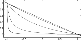
Figure 1: The shape of the interpolation function $\alpha_{\varepsilon}$ for $q=10^{i},i=-2,\ldots 2$ (bottom to top).

To fulfill Assumption (A5) we cut $\alpha_{\varepsilon}$ at $\varphi\equiv\varphi_{c}>1$ and use any smooth continuation yielding $\alpha_{\varepsilon}(\varphi)\equiv\mbox{const}$ for $\varphi\geq\varphi_{c}$.

The parameter $q$ controls the width of the transition zone between fluid and porous material. In [6] the authors typically use a rather small value of $q=0.01$. They also show how different values of $q$ might lead to different local optimal topologies. Since here we also have the parameter $\varepsilon$ for controlling the maximal width of the transition zone we fix $q:=10$.

The fluid material is assumed to be located at $\varphi=1$ where $\alpha(1)=0$ holds. Since we use Moreau–Yosida relaxation we allow $\varphi$ to take values larger then $+1$ and smaller then $-1$. The choice of $q=10$ and $s=10^{6}$ in our setting always guarantees, that $\varphi+1+q\gg 0$ holds, and that the violation of $\alpha_{\varepsilon}(\varphi)\geq 0$ at $\varphi=1$ only is small.

Using an interpolation function that yields a smooth transition to zero at $\varphi=1$, say a polynomial of order 3, in our numerics especially for small values of $\gamma$ yields undesired behaviour of the numerical solvers. We for example obtain that fluid regions disappear resulting in a constant porous material. The reason is, that then $\alpha_{\varepsilon}(\beta)\approx 0$ if $\beta$ is chosen in the flat region of $\alpha_{\varepsilon}$. If $\beta$ can be chosen small enough, the choice of $\varphi\equiv\beta$ yields constant porous material and hence a very small total potential power. Thus, $\varphi\equiv\beta$ is at least a local minimizer.

The benefit of small values of $q$ described in [6] stays valid and for large values of $\gamma$, say $\gamma=1$, small values of $q$ can help finding a valid topology when starting from a homogeneous material. This property is the reason to use this function instead of a linear one, although $\alpha_{\varepsilon}$ can be regarded as linear for the value of $q=10$ that we use here.

4.3.1 The influence of $\overline{\alpha}_{\varepsilon}$ on the interface

The separating effect not only arises from the contribution of the Ginzburg–Landau energy, but also the term $\alpha_{\varepsilon}(\varphi)\left(\frac{1}{2}|\boldsymbol{u}|^{2}-\boldsymbol{u}\cdot\boldsymbol{q}\right)$ yields the demixing of fluid and porous material. Since $\alpha_{\varepsilon}$ scales with $\overline{\alpha}_{\varepsilon}$ we next investigate the relative effect of $\overline{\alpha}$ and $\varepsilon$ concerning the demixing and thus the width of the resulting interface. This is done for several values of the parameter $\gamma$, which weights the two separating forces.

The numerical setup for this test is described in the following. In the computational domain $\Omega=(0,1)^{2}$ we have a parabolic inlet at $x\equiv 0$ with $m=0.5,l=0.2$, and $h=1$. At $x\equiv 1$ we have an outlet with the same values. The viscosity is set to $\mu=1$. We investigate the evolution of the value

$$I=\frac{\int_{\{|\varphi|\leq 1\}}\,\mathrm{d}x}{\int_{\{\varphi=0\}}\,\mathrm{d}s},$$

which is the size of the area of the transition zone between fluid and material, and which is normalized by the length of the interface. This value estimates the thickness of the interfacial region. For this test we fix $\varepsilon\equiv 1$ in (23) and use the interpolation function

$$\alpha(\varphi)=\alpha_{1}(\varphi)=\frac{\overline{\alpha}}{2}(1-\varphi)\frac{q}{(\varphi+1+q)},$$

so that $\overline{\alpha}\equiv\alpha(-1)$.

For fix $\gamma$ we calculate the optimal topology for several combinations of $\varepsilon$ and $\overline{\alpha}$. In Figure 2 we depict the value of $I$ depending on $\overline{\alpha}$ for several $\varepsilon$. We used $\gamma\in\{0.5,0.05,0.005\}$ (left to right).

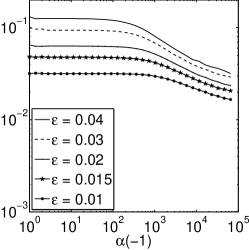
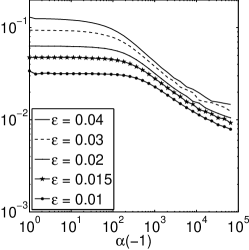
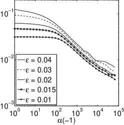
Figure 2: Size of the scaled interfacial area for various combinations of $\overline{\alpha}=\alpha(-1)$ and $\varepsilon$, with $\gamma=0.5$ (left), $\gamma=0.05$ (middle) and $\gamma=0.005$ (right).

We observe that there is a regime of values for $\overline{\alpha}$ where the interfacial width only depends on $\varepsilon$. But we also see, that, depending on $\gamma$ and $\varepsilon$, there is a regime where the interfacial width scales like $\overline{\alpha}^{\kappa}$ with some $\kappa\in\mathbb{R}$ which depends on $\gamma$.

The change in the behaviour of the interfacial width occurs at $\alpha(-1)\approx C(\gamma)\varepsilon^{-1}$, where $C(\gamma)$ is a constant depending linearly on $\gamma$. This is exactly the convergence rate necessary to get analytical convergence results, compare Remark 2 and [27].

We recall that this test is run with constant $\mu=1$ and that the results might differ for different values of $\mu$. In particular the value of $\mu$ also has an influence on the interfacial width through the mixing energy $\frac{1}{2}|\boldsymbol{u}_{h}|^{2}-\boldsymbol{u}_{h}\cdot\boldsymbol{q}_{h}$, see Section 4.5.3.

4.4 A treelike structure

In this first example we investigate how our phase field approach is able to find optimal topologies starting from a homogeneous porous material. This example is similar to an example provided in [22]. The setup is as follows. The computational domain is $\Omega=(0,1)^{2}$. On the boundary we have one parabolic inlet as described in (22) and four parabolic outlets. The corresponding parameters are given in Table 1.

direction	boundary	m	l	h
inflow	$\{x\equiv 0\}$	0.80	0.2	3
outflow	$\{y\equiv 0\}$	0.80	0.1	1
outflow	$\{y\equiv 1\}$	0.65	0.1	1
outflow	$\{x\equiv 1\}$	0.70	0.2	1
outflow	$\{x\equiv 1\}$	0.25	0.2	1

Table 1: Boundary data for the treelike structure.

We use $\gamma=0.01$ and $\mu=0.01$. For $\alpha_{\varepsilon}$ we start with $\overline{\alpha}=5$ and increase it later. The phase field is initialized with a homogeneous porous material $\varphi_{0}=0$. We start with a homogeneous mesh with mesh size $2e-5$ to obtain a first guess of the optimal topology. After the material demixes, i.e. $\|\nabla w^{h}\|_{\boldsymbol{L}^{2}(\Omega)}\leq 2$, we start with adapting the mesh to the resulting structures using the adaptation procedure described in Section 3.1.1. For the adaptive process we use the parameter $a_{\min}=4e-7$, $a_{\max}=0.01$, $\theta^{r}=0.1$, and $\theta^{c}=0.05$. As soon as $\|\nabla w^{h}\|_{\boldsymbol{L}^{2}(\Omega)}\leq 1$ holds we start with increasing $\overline{\alpha}$ to $\overline{\alpha}=50$ and stop the allover procedure as soon as $\overline{\alpha}=50$ and $\|\nabla w^{h}\|_{\boldsymbol{L}^{2}(\Omega)}\leq 1e-5$ holds.

In Figure 3 we depict the temporal evolution of the optimization process. The images are numbered from top left to bottom right. Starting from a homogeneous distribution of porous material, we see that the inlet and the outlets are found after very few time instances and that the main outlets on the right and the inlet are connected after only a few more time steps. At the bottom left of the computational domain we first obtain finger like structures that thereafter vanish. We note that, due to the porous material approach, not all outlets are connected with the inlet during the whole computation. At the final stage of the optimization the evolution slows down and we end with the topology depicted at the bottom right after 188 time steps of simulation.

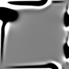
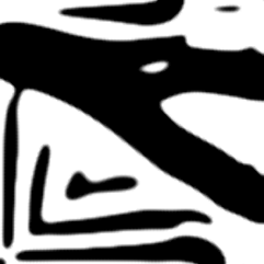
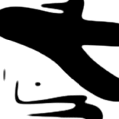
Figure 3: The initial phase field $\varphi_{0}$ for the treelike structure and the phase field after 6, 12, 36, 70, and 188 time steps (top left to bottom right).

4.5 A rugby ball

We next investigate the overall behaviour of the adaptive concept and give an example showing the influence of the parameters $\gamma$ and $\mu$ on the interfacial area. The aim is to optimize the shape of a ball in an outer flow as is investigated in [6, 37, 39].

In the computational domain $\Omega=(0,1)\times(0,5)$ we have a circle located at $M=(0.5,0.5)$ with radius $r=\sqrt{(10\pi)^{-1}}$. On the boundary $\partial\Omega$ we impose Dirichlet data $\boldsymbol{g}\equiv(0,1)^{T}$ for the Navier–Stokes equations. The domain is chosen large enough to neglect the influence of the outflow boundary on the optimized topology.

In [6] it is shown that for Stokes flow the optimal topology equals a rugby ball, while in [37, 39] the authors obtain an airfoil-like shape for Navier–Stokes flow and small values of $\mu$. The parameters used here are $\varepsilon=0.005$ and $\overline{\alpha}=50$. For the adaptive concept we fix $\theta^{r}=0.2$, $\theta^{c}=0.05$, $a_{\min}=10^{-7}$ and $a_{\max}=5\cdot 10^{-4}$. As initial mesh we use a homogeneous mesh with mesh size $a_{\text{init}}=1/1600$ and refine the region $|\varphi_{0}|\leq 1$ to the finest level, where $\varphi_{0}$ denotes the initial phase field.

4.5.1 Optimal shapes for various $\gamma$ and $\mu$

We start with depicting our numerical findings for various values of $\gamma$ and $\mu$. Here we proceed as follows. We optimize the shape for decreasing values of $\gamma\in[10^{-4},10]$ and $\mu=1$. The optimal geometry for $\mu=1$ and $\gamma=10^{-4}$ thereafter is used as initial value for decreasing $\mu\in[500^{-1},1]$ while $\gamma=10^{-4}$ is kept fix. In Figure 4 we depict the optimal shapes for $\mu=1$ and $\gamma\in\{10,0.1,0.01,0.0001\}$, and in Figure 5 we depict the optimal shapes for $\gamma=10^{-4}$ and $\mu\in\{10^{-1},100^{-1},300^{-1},500^{-1}\}$.

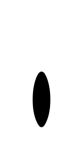
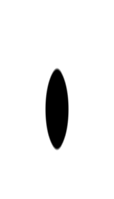
Figure 4: Optimal topologies for the rugby ball example for $\mu=1$ and $\gamma\in\{10,0.1,0.01,0.0001\}$ (left to right).

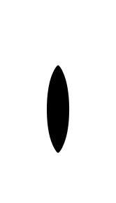
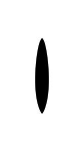
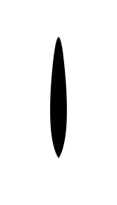
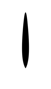
Figure 5: Optimal topologies for the rugby ball example for $\gamma=10^{-4}$ and $\mu\in\{10^{-1},100^{-1},300^{-1},500^{-1}\}$ (left to right).

We see that for large values of $\gamma$ the Ginzburg–Landau energy dominates the minimizing problem and thus we obtain an optimal shape which is close to a circle. With $\gamma$ getting smaller we obtain shapes that resemble rugby balls like shapes as obtained in [6] for the Stokes flow. In particular we see that the top and bottom tip get sharper as we decrease the value of $\gamma$. This can be explained by the Ginzburg–Landau energy. This term penalises the interfacial size and explains why for large values of $\gamma$ the optimal shape is close to a circle. Note that the optimal shape can locate freely in the computational domain and therefore the optimal shape for $\gamma=10^{-4}$ has a slightly larger distance to the bottom boundary than the optimal shapes for larger $\gamma$.

As argued in [37], for $\mu$ taking smaller values, the optimal shape tends to an airfoil. This is what we observe in our numerics, see Figure 5.

For a quantitative description of the optimal shapes we follow [39, Rem. 12] and introduce the friction drag of an obstacle in free flow as

$$F_{D}=\int_{\{\varphi=0\}}-\mu\left(\left(\nu\cdot\nabla\right)\boldsymbol{u}\right)\cdot a+p\nu\cdot a\,\mathrm{d}s.$$ (24)

Here $\nu$ is the unit normal on the boundary of the ball pointing inwards and $a$ is the direction of attack of the flow field. In our example we have $a=(0,1)^{T}$ since the flow is attaining from the bottom. By using the Gauss theorem we write $F_{D}$ as an integral over the ball given by $\varphi<0$ and obtain

$$F_{D}=-\int_{\{\varphi<0\}}\,\mathrm{div}\,\left(-\mu\nabla u_{2}+(0,p)^{T}\right)\,\mathrm{d}x=-\int_{\{\varphi<0\}}-\mu\Delta u_{2}+p_{y}\,\mathrm{d}x.$$ (25)

Note that the normal $\nu$ in (24) points into the rugby ball and thus we obtain the minus sign in (25). Here $u_{2}$ denotes the second component of the velocity field $\boldsymbol{u}$ and $p_{y}$ denotes the derivative of $p$ in $y$-direction.

As second comparison value we define the circularity of the rugby ball. This value is introduced in [41] to describe the deviation of circular objects from a circle. It is defined by

$$\theta=\frac{\mbox{Circumference of circle with same area}}{\mbox{Circumference of object}}=\frac{\sqrt{4\pi\int_{\{\varphi<0\}}\,\mathrm{d}x}}{\int_{\{\varphi=0\}}\,\mathrm{d}s}\leq 1,$$ (26)

where a value of $\theta\equiv 1$ indicates a circle.

In Table 2 we give results for our numerical findings.

$\gamma$	$\mu$	$F$	$\theta$	$F_{D}$
10.0000	1	7.2266	0.9996	21.6140
1.0000	1	6.5317	0.9664	18.5820
0.1000	1	6.1828	0.8005	16.6710
0.0100	1	6.1494	0.7722	16.4640
0.0010	1	6.1480	0.7681	16.4510
0.0001	1	6.1427	0.7674	16.4310

$\gamma$	$\mu$	$F$	$\theta$	$F_{D}$
0.0001	10-1	1.1353	0.7335	2.3596
0.0001	100-1	0.1830	0.6349	0.3244
0.0001	200-1	0.1188	0.5901	0.1910
0.0001	300-1	0.0942	0.5568	0.1395
0.0001	400-1	0.0805	0.5403	0.1114
0.0001	500-1	0.0715	0.5253	0.0930

Table 2: Comparison values for the rugby example. $F$ is the dissipative power, $\theta$ denotes the circularity, and $F_{D}$ the drag force. The optimization aim is the minimization of the dissipative power.

As discussed above for large values of $\gamma$ the Ginzburg–Landau energy dominates the functional under investigation. This results in optimal shapes that are close to circles as can be seen for $\gamma=1$ and $\gamma=1$ where we have $\theta=1$ and $\theta=0.97$ respectively. We further see that for $\gamma=0.01$ the optimal shape is determined by the dissipative power, since the results for $\gamma=0.01$ and $\gamma=0.0001$ are very close together. Concerning the dependence with respect to $\mu$ we see how the dissipative energy, which scales with $\mu$, decreases with decreasing $\mu$. We also obtain that both the circularity and the drag are reduced for smaller values of $\mu$. For the drag we have approximately $F_{D}\sim\mu^{0.84}$.

4.5.2 Behaviour of the adaptive concept

Next we investigate the behaviour of the adaptive concept. Since the error indicators only contain the jumping terms of the gradient, we expect the indicators mainly to be located at the borders of the interface, i.e. the isolines $\varphi=\pm 1$. In Figure 6 we depict the distribution of the error indicator $\eta_{T_{E}}$ for the optimal topology for $\gamma=10^{-4}$ and $\mu=1$.

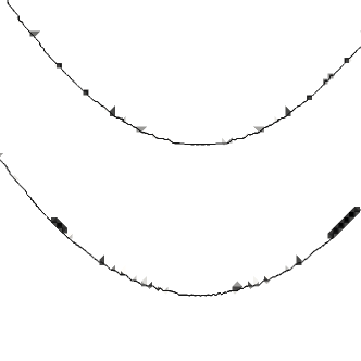
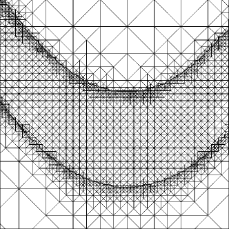
Figure 6: The bottom arc of the rugby ball for $\gamma=10^{-4}$ and $\mu=1$. The distribution of $\eta_{T_{E}}$ across the interface is shown in the left plot, where darker areas indicate larger error. The spatial resolution of the interface is depicted in the right plot. The bold lines indicate the discrete sets $\varphi\equiv\pm 1$.

We observe from the left plot, that the indicator $\eta_{T_{E}}$ is concentrated at the discrete isolines $\varphi=\pm 1$. Here the mesh is refined to the finest level as we see in the right plot. Inside the interface the triangles are only mildly refined. Here the phase field tends to be linear and thus a high spatial resolution is not required to get a well resolved phase field.

4.5.3 A view on mixing energy

From the point of view of Cahn–Hilliard theory, (17) alone for fixed vector fields $\boldsymbol{u},\boldsymbol{q}$ can be regarded as the Cahn–Hilliard system with a free energy $F$ given by

$$F(\varphi)=\frac{\gamma}{\varepsilon}(1-\varphi^{2})+\frac{s}{2}\lambda^{2}(\varphi)+\alpha_{\varepsilon}(\varphi)\left(\frac{1}{2}|\boldsymbol{u}|^{2}-\boldsymbol{u}\cdot\boldsymbol{q}\right).$$ (27)

The term $\frac{1}{2}|\boldsymbol{u}|^{2}-\boldsymbol{u}\cdot\boldsymbol{q}$ is assumed to be non negative. For $F$ we require two distinct minima located at $\approx\pm 1$. If $|\varphi|>1$ holds it is reasonable to assume that $s\lambda^{2}(\varphi)$ is the dominating term and in the ongoing we investigate the distribution of $F$ inside the interface defined by $|\varphi|\leq 1$. We note that this distribution in fact depends on $\gamma,\varepsilon,\overline{\alpha}$, and $\mu$. As in Section 4.2 we fix $\varepsilon$ to be $0.005$. Since both $\overline{\alpha}$ and $\gamma$ give a weighting of the two energy terms we also fix $\overline{\alpha}\equiv 50$ as proposed in Section 4.3. Thus the free parameters in this investigation are $\gamma$ and $\mu$.

In Figure 7 we show the distribution of the terms $\alpha_{\varepsilon}(\varphi)(\frac{1}{2}|\boldsymbol{u}|^{2}-\boldsymbol{u}\cdot\boldsymbol{q})$ and $\frac{\gamma}{\varepsilon}(1-\varphi^{2})$ at the bottom arc of the optimized rugby ball.

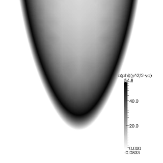
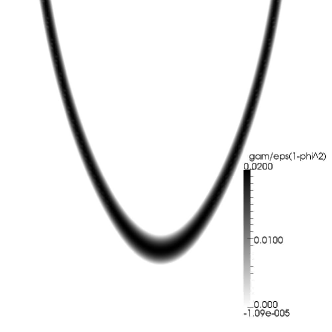
Figure 7: The energies $\alpha_{\varepsilon}(\varphi)(\frac{|\boldsymbol{u}|^{2}}{2}-\boldsymbol{u}\cdot\boldsymbol{q})$ (left plot) and $\frac{\gamma}{\varepsilon}(1-\varphi^{2})$ (right plot) at the bottom of the optimized topology for $\gamma=10^{-4}$ and $\mu=1$.

We see, that the term $\alpha_{\varepsilon}(\varphi)(\frac{1}{2}|\boldsymbol{u}|^{2}-\boldsymbol{u}\cdot\boldsymbol{q})$ is larger then $\frac{\gamma}{\varepsilon}(1-\varphi^{2})$ and thus dominates the demixing. The term admits a maximum inside the interface and takes smaller values outside of the interface. We note that the term $\frac{\gamma}{\varepsilon}(1-\varphi^{2})$ is symmetric across the interface, while $\alpha_{\varepsilon}(\varphi)(\frac{1}{2}|\boldsymbol{u}|^{2}-\boldsymbol{u}\cdot\boldsymbol{q})$ takes its maximum near $\varphi=-1$ and especially also takes large values inside the porous material.

4.6 An optimal embouchure for a bassoon

As outlook we investigate the optimal shape of an embouchure for a bassoon. In the group of Professor Grundmann at the Technische Universität Dresden by experiments an optimized shape was found that has a smaller pressure loss along the pipe, while it only slightly changes the sound of the bassoon, see [25].

We apply our optimization algorithm to the problem of finding an optimal embouchure in order to illustrate possible fields of application of our approach. We note that again we minimize the dissipative energy, and that we do not take further optimization constraints into account.

We proceed as described in Section 4.4 to find optimal shapes in $\Omega=(0,1)^{2}$ for the parameters $\gamma=1e-4$, $\varepsilon=0.005$, $\overline{\alpha}=50$ and $\mu=1e-3$. We start with a constant initial phase field using $\beta=0.1$. The inflow is set to $x\equiv 1$ and we use the parameters $m_{i}=0.5$, $l_{i}=0.1$, $h_{i}=1$ in (22) both for the $x$ and $y$ direction of the boundary velocity field, resulting in an inflow pointing $45\degree$ upwards. We set the outflow to $y\equiv 0$ and consider two scenarios. For the first scenario we use the values $m_{1}=0.8$, $l_{1}=0.2$ and $h_{1}=0.5$ in (22), and for the second example we use $m_{2}=0.3$, $l_{2}=0.2$ and $h_{2}=0.5$.

In Figure 8 we show our numerical finding. We obtain a straight and wide pipe that directly connects inflow and outflow boundary. This corresponds to our optimization aim, i.e. minimizing the dissipative power. Similar trends for the optimized shape of the embouchure were also observed by the group in Dresden.

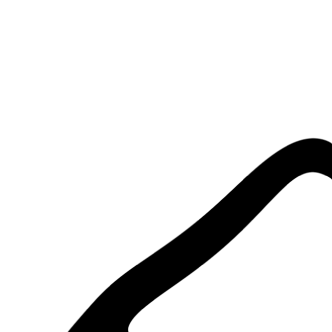
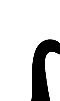
Figure 8: Optimized shapes for the bassoon example for $\mu=1000^{-1}$. First scenario on left side, second scenario on right side. The inflow is on the right side.

References

- [1] M. Ainsworth and J. T. Oden. A Posteriori Error Estimation in Finite Element Analysis. Wiley, September 2000.
- [2] L. Ambrosio and G. Buttazzo. An optimal design problem with perimeter penalization. Calc. Var. Partial Differential Equations, 1(1):55–69, 1993.
- [3] M.P. Bendsøe, R.B. Haber, and C.S. Jog. A new approach to variable-topology shape design using a constraint on perimeter. Struct. Multidiscip. Optim., 11(1-2):1–12, 1996.
- [4] M. Benzi, G.H. Golub, and J. Liesen. Numerical solution of saddle point problems. Acta Numer., 14:1–137, 2005.
- [5] L. Blank, H. Farshbaf-Shaker, H. Garcke, and V. Styles. Relating phase field and sharp interface approaches to structural topology optimization. to appear in ESAIM: COCV, 2014.
- [6] T. Borrvall and J. Petersson. Topology optimization of fluids in Stokes flow. Internat. J. Numer. Methods Fluids, 41(1):77–107, 2003.
- [7] J. Bosch, M. Stoll, and P. Benner. Fast solution of Cahn-Hilliard Variational Inequalities using Implicit Time Discretization and Finite Elements. J. Comput. Phys., 2014.
- [8] B. Bourdin and A. Chambolle. Design-dependent loads in topology optimization. ESAIM Control Optim. Calc. Var., 9:19–48, 8 2003.
- [9] C. Brandenburg, F. Lindemann, M. Ulbrich, and S. Ulbrich. A Continuous Adjoint Approach to Shape Optimization for Navier Stokes Flow. In K. Kunisch, J. Sprekels, G. Leugering, and F. Tröltzsch, editors, Optimal Control of Coupled Systems of Partial Differential Equations, volume 158 of Internat. Ser. Numer. Math., pages 35–56. Birkhäuser, 2009.
- [10] C. Brandenburg, F. Lindemann, M. Ulbrich, and S. Ulbrich. Advanced Numerical Methods for PDE Constrained Optimization with Application to Optimal Design in Navier Stokes Flow. In G. Leugering, S. Engell, A. Griewank, M. Hinze, R. Rannacher, V. Schulz, M. Ulbrich, and S. Ulbrich, editors, Constrained Optimization and Optimal Control for Partial Differential Equations, pages 257–275. Birkhäuser, 2012.
- [11] M. Burger and R. Stainko. Phase-field relaxation of topology optimization with local stress constraints. SIAM J. Control Optim., 45:1447–1466, 2006.
- [12] C. Carstensen. Quasi-interpolation and a-posteriori error analysis in finite element methods. ESAIM Math. Model. Numer. Anal., 33(6):1187–1202, 1999.
- [13] C. Carstensen and R. Verfürth. Edge Residuals Dominate A Posteriori Error Estimates for Low Order Finite Element Methods. SIAM J. Numer. Anal., 36(5):1571–1587, 1999.
- [14] T. A. Davis. Algorithm 832: Umfpack v4.3 - an unsymmetric-pattern multifrontal method. ACM Trans. Math. Software, 30(2):196–199, 2004.
- [15] W. Dörfler. A convergent adaptive algorithm for Poisson’s equation. SIAM J. Numer. Anal., 33(3):1106–1124, 1996.
- [16] L.C. Evans and R.F. Gariepy. Measure Theory and Fine Properties of Functions. Mathematical Chemistry Series. CRC PressINC, 1992.
- [17] A. Evgrafov. The Limits of Porous Materials in the Topology Optimization of Stokes Flows. Appl. Math. Optim., 52(3):263–277, 2005.
- [18] A. Evgrafov. Topology optimization of slightly compressible fluids. ZAMM Z. Angew. Math. Mech., 86(1):46–62, 2006.
- [19] D. J. Eyre. Unconditionally gradient stable time marching the Cahn–Hilliard equation. In Computational and Mathematical Models of Microstructural Evolution, volume 529 of MRS Proceedings, 1998.
- [20] G.P. Galdi. An Introduction to the Mathematical Theory of the Navier-Stokes Equations. Springer, 2011.
- [21] H. Garcke, M. Hinze, and C. Kahle. A stable and linear time discretization for a thermodynamically consistent model for two-phase incompressible flow. arXiv: 1402.6524, 2014.
- [22] A. Gersborg-Hansen. Topology optimization of flow problems. PhD thesis, Technical University of Denmark, 2007.
- [23] V. Girault and P. A. Raviart. Finite Element Methods for Navier–Stokes Equations, volume 5 of Springer series in computational mathematics. Springer, 1986.
- [24] E. Giusti. Minimal surfaces and functions of bounded variation. Notes on pure mathematics. Dept. of Pure Mathematics, 1977.
- [25] R. Grundmann. Das Fagott und die Strömungsmechanik. Forschung, 29(1):16–17, 2004.
- [26] A. G. Hansen, O. Sigmund, and R. B. Haber. Topology optimization of channel flow problems. Struct. Multidis. Optim., 30:181–192, 2005.
- [27] C. Hecht. Shape and topology optimization in fluids using a phase field approach and an application in structural optimization. Dissertation, University of Regensburg, 2014.
- [28] M. Hintermüller, M. Hinze, and C. Kahle. An adaptive finite element Moreau–Yosida-based solver for a coupled Cahn–Hilliard/Navier–Stokes system. J. Comput. Phys., 235:810–827, February 2013.
- [29] M. Hintermüller, M. Hinze, and M.H. Tber. An adaptive finite element Moreau–Yosida-based solver for a non-smooth Cahn–Hilliard problem. Optim. Methods Softw., 25(4-5):777–811, 2011.
- [30] B. Kawohl, A. Cellina, and A. Ornelas. Optimal Shape Design: Lectures Given at the Joint C.I.M./C.I.M.E. Summer School Held in Troia (Portugal), June 1-6, 1998. Lecture Notes in Mathematics / C.I.M.E. Foundation Subseries. Springer, 2000.
- [31] D. Kay, D. Loghin, and A. Wathen. A preconditioner for the steady state Navier–Stokes equations. SIAM J. Sci. Comput., 24(1):237–256, 2002.
- [32] S. Kreissl and K. Maute. Levelset based fluid topology optimization using the extended finite element method. Struct. Multidis. Optim., 46:311–326, 2012.
- [33] L. Modica. The gradient theory of phase transitions and the minimal interface criterion. Arch. Ration. Mech. Anal., 98(2):123–142, 1987.
- [34] B. Mohammadi and O. Pironneau. Shape optimization in fluid mechanics. Annu. Rev. Fluid Mech., 36:255–279, 2004.
- [35] L. H. Olesen, F. Okkels, and H. Bruus. A high-level programming-language implementation of topology optimization applied to steady state Navier-Stokes flow. Internat. J. Numer. Methods Engrg., 65(7):975–1001, 2006.
- [36] L. E. Payne and H. F. Weinberger. An optimal Poincaré inequality for convex domains. Arch. Ration. Mech. Anal., 5(1):286–292, Januar 1960.
- [37] G. Pingen, A. Evgrafov, and K. Maute. Topology optimization of flow domains using the lattice Boltzmann method. Struct. Multidis. Optim., 34:507–524, 2007.
- [38] Y. Saad and M. H. Schultz. GMRES: A generalized minimal residual algorithm for solving nonsymmetric linear systems. SIAM Journal on Scientific and Statistical Computing, 7(3):856–869, July 1986.
- [39] S. Schmidt and V. Schulz. Shape Derivatives for General Objective Functions and the Incompressible Navier–Stokes Equations. Control Cybernet., 39(3):677–713, 2010.
- [40] V. Sv̌erák. On optimal design. J. Maths. Pures Appl., 72:537–551, 1993.
- [41] H. Wadell. Spericity and Roundness of Rock Particles. The Journal of Geology, 41(3):310–331, 1933.