Mining the gap: evolution of the magnitude gap in X-ray galaxy groups from the 3 square degree XMM coverage of CFHTLS

We present a catalog of 129 X-ray galaxy groups, covering a redshift range 0.04$<$z$<$1.23, selected in the $\sim$3 degree² part of the CFHTLS W1 field overlapping XMM observations performed under the XMM-LSS project. We carry out a statistical study of the redshift evolution out to redshift one of the magnitude gap between the first and the second brightest cluster galaxies of a well defined mass-selected group sample. We find that the slope of the relation between the fraction of groups and the magnitude gap steepens with redshift, indicating a larger fraction of fossil groups at lower redshifts. We find that 22.2$\pm$6% of our groups at z$\leq$0.6 are fossil groups. We compare our results with the predictions of three semi-analytic models based on the Millennium simulation. The intercept of the relation between the magnitude of the brightest galaxy and the value of magnitude gap becomes brighter with increasing redshift. This trend is steeper than the model predictions which we attribute to the younger stellar age of the observed brightest cluster galaxies. This trend argues in favor of stronger evolution of the feedback from active galactic nuclei at z$<$1 compared to the models. The slope of the relation between the magnitude of the brightest cluster galaxy and the value of the gap does not evolve with redshift and is well reproduced by the models, indicating that the tidal galaxy stripping, put forward as an explanation of the occurrence of the magnitude gap, is both a dominant mechanism and is sufficiently well modeled.

1 Introduction

Groups and clusters are important environments for the formation and evolution of galaxies, particularly for the very bright galaxies. In the last few decades, several observational and theoretical studies have focused on the group and cluster environments in order to advance our understanding of their galaxy properties (e.g., White & Rees 1978; Yang et al. 2005; Yang et al. 2008; Yang et al. 2009; Zandivarez et al. 2006; Zibetti et al. 2009; Percival et al. 2010; van den Bosch et al. 2013; Hearin et al. 2013; Scoville et al. 2007).

While effects of gravity on galaxy formation have been modeled in great detail (e.g., Zel’dovich 1970; Weinberg 1972; Press & Schechter 1974; Huntley 1980; Barnes 1989; Bekki et al. 2002; Libeskind et al. 2006; Junqueira et al. 2013), processes of the galaxy evolution are also governed by the gas content available for star-formation. For galaxies in groups and clusters, the cold gas content depends on both external (cooling of the intracluster medium (ICM), gas stripping by galactic motion through ICM, observed even for the central galaxy due to sloshing), and internal processes galactic outflows, driven by the feedback from active galactic nuclei (AGN) and supernovae (Croton et al. 2006). In addition, the central galaxy can grow by merging and tidal stripping of satellite galaxies.

Dynamical friction causes massive galaxies in halos with sufficiently low velocity dispersion to merge in a few Gyrs with the central group galaxy, forming a giant elliptical galaxy (Ponman et al. 1994). Within this galaxy-galaxy merger paradigm, luminosity gap may be sensitive to merger rates in groups and clusters of galaxies. To get the insights on the processes associated with the formation of central galaxies, we embark on a study of the occurrence of the magnitude gap.

The magnitude gap is often used to study the formation history and dynamical age of the hosting halo, particularly in fossil groups (Milosavljević et al. 2006; van den Bosch et al. 2007; Dariush et al. 2007). Simulations of D’Onghia et al. (2005) show that early formed groups ( , fossils) have larger magnitude gaps. Tracing fossil groups forward in time, Von Benda-Beckmann et al. (2008) find that their large magnitude gaps can be filled by a recent infall of galaxies. Also, some merger events may not be caught by the gap statistics, as indicated by a study of La Barbera et al. (2012). Thus, to derive conclusions from the gap statistics, a comparison to numerical simulations is required. To date, such a comparison has only been performed on the nearby galaxy groups at z$\sim$0 and massive clusters at z$\sim$0.2 (Dariush et al. 2010; Smith et al. 2010). This paper expands the studies of the cosmic evolution of the magnitude gap to a redshift of 1.1.

To the extremes of the magnitude gap characterization belong the fossil groups, which have L${}_{X}\gtrsim$2.13$\times$10⁴² h^-2erg s^-1 and a magnitude gap above $\Delta M_{1,2}$=2 mag (Jones et al. 2003). Origin and nature of fossil groups are still not completely understood. Identification of these systems is challenging, and further studies and observations (i.e., X-ray and spectroscopic) of fossil groups are of interest. According to Jones et al. (2003), 8 to 20 per cent of all galaxy groups are fossils. Simulations suggest that fossils tend to reside in less dense environments compared to an average group of similar total mass and formation history D’Onghia et al. (2005); Dariush et al. (2007); Díaz-Giménez et al. (2011). This is also observed in the environmental study of a fossil group, ESO 3060170 (Su et al. 2013). Fossil galaxy groups have been shown to exhibit interesting properties such as concentrated dark matter halos (Khosroshahi et al. 2007; Humphrey et al. 2012), disky isophotes of the central galaxies (Khosroshahi et al. 2006; Smith et al. 2010). From the age and metallicity gradients of fossils, in a study based on six galaxies Eigenthaler & Zeilinger (2013) concluded that these systems form by multiple mergers of massive galaxies.

Identification and detection of galaxy groups is also challenging, since the overdensity of galaxies per unit area in a redshift slice is more sensitive to the projection effects by foreground and background galaxies compared to clusters. In addition, to study the galaxy properties it is advantageous to have a group selection that is independent of galaxy properties. Extended X-ray emission from groups and clusters of galaxies offers such a selection (Borgani & Guzzo 2001; Rosati et al. 2002). Deep XMM and Chandra surveys such as Chandra Deep Field South (CDFS; Giacconi et al. 2002), Chandra Deep Field North (CDFN; Bauer et al. 2002), Lockman Hole (Finoguenov et al. 2005), the Cosmic Evolution Survey (COSMOS; Finoguenov et al. 2007), XMM-Large Scale Structure (LSS; Pacaud et al. 2007), the Canadian Network for Observational Cosmology (CNOC2; Finoguenov et al. 2009; Connelly et al. 2012), Subaru-XMM Deep Field (SXDF; Finoguenov et al. 2010), the XMM-Newton-Blanco Cosmology Survey project (XMM-BCS; Šuhada et al. 2012) reveal new capabilities of X-ray selection of groups. Catalogs available from these surveys have already made an important contribution to studies of galaxy formation and evolution (e.g., Tanaka et al. 2008, 2012; Giodini et al. 2009; Silverman et al. 2009; Allevato et al. 2012).

The main goal of this paper is to identify X-ray galaxy groups in the part of the CFHTLS W1 field covered by XMM observations. We carry out a statistical study of the redshift evolution, up to a redshift of 1.1, of the magnitude gap and the volume abundance of the detected X-ray galaxy groups. We combine the observational measurements of the distribution of the luminosity gap of groups and the absolute magnitude of the brightest galaxies, and compare this to predictions of semi-analytic models (SAMs) from Bower et al. (2006, hereafter B06), De Lucia & Blaizot (2007, hereafter DLB07) and Guo et al. (2011, hereafter G11). The study of magnitude gap statistics and X-ray properties of galaxy groups enable us to identify fossil group candidates in our sample. We also report on the redshift evolution of the extent of X-ray detection from galaxy groups.

The structure of this paper is as follows: we present the XMM-Newton and CFHTLS data in §2. §3 gives a brief description of the SAMs we use in this paper, highlighting their differences and similarities. In §4, we describe the group identification technique and present a catalog of galaxy groups. §5 discusses group membership contamination. We present magnitude gap statistics and relation between the magnitude of the first and second brightest group galaxies (BGGs) and the magnitude gap in §6. We summarize our results in §7.

Unless stated otherwise, we adopt a ‘concordance’cosmological model, with ($\Omega_{\Lambda},\Omega_{M}$, h)=(0.75, 0.25, 0.71), where the Hubble constant is characterized as 100 h km s^-1 Mpc^-1 and quote uncertainties on 68% confidence level.

2 Data

2.1 XMM-Newton data

A description of the XMM–Newton observatory is given by Jansen et al. (2001). We use the data collected by the European photon imaging cameras (EPIC): the pn-CCD camera (Strüder et al. 2001) and the MOS-CCD cameras (Turner et al. 2001).

In this paper we analyzed the XMM-Newton observations of the CFHTLS wide (W1) field as a part of the XMM–LSS survey Pierre et al. (2007). The details of observations and data reduction are presented in Bielby et al. (2010). We concentrate on the low-z counterparts of the X-ray sources and use all XMM observations performed till 2009, covering an area of 2.276${}^{\circ}\times$2.276^∘. Altogether, $\sim$3 degrees² of this area is covered by the optical data of the CFHTLS survey. The primary cluster catalog of the XMM-LSS project is published in Adami et al. (2011). The group catalog presented in this paper extends the Adami et al. (2011) work to low-mass systems, as well as presents X-ray flux estimates with contribution from point sources removed. This allows us to self-consistently infer cluster masses, using the calibrations achieved in the COSMOS survey using a similar flux extraction technique (Leauthaud et al. 2010). In our modeling of the survey sensitivity, we account for both the variation in the exposure due to differences in the flare removal, vignetting, and the aperture flux loss for nearby groups.

The modeling of the flux limit is defined by the spatial scales used for the detection and the sensitivities achieved on these scales. The change in the flux limit with redshift occurs at redshifts below 0.2 and is due to the correction for the missing flux, while the aperture flux limit is considered to be redshift independent. The correction for the missing flux is done following the tabulations of Finoguenov et al. (2007).

In Fig. 1 we present the flux limit corresponding to the best 10% (solid red curve) and 90% (dotted blue curve) of the area. In addition to an increase in the flux, very low-z systems are hard to identify in the photometric data due to the projection effects. The volume covered at low-z (e.g., z $<0.05$) is very small, 0.02% of the total survey volume, while formal galaxy group luminosities are below $10^{41}$ ergs s^-1 level, beyond the explored level for galaxy groups. The dashed black horizontal line in Fig.1 illustrates the $10^{-14}$ ergs s^-1 cm ^-2 flux threshold adopted for the C1 XMM-LSS sample (Pacaud et al. 2007). The open black squares with error bars show our flux (ergs s^-1 cm ^-2, 0.5–2 keV band) estimates versus redshift. We show 30 galaxy groups in common with Adami et al. (2011) with filled blue squares. These 30 galaxy groups include one system from C0, all 17 systems from C1 which are within the CFHTLS coverage, five systems from C2 and seven systems from C3 in the XMM-LSS classification. Using simulations, Pacaud et al. (2006) classified extended sources as C1 and C2. The C1 class is a purely X-ray selected cluster (i.e., less than 1% of clusters can be found as miss-classified point-like source). The C2 class allows for the 50% contribution from the miss-classified point-liked sources. The C3 clusters are classified as faint objects with less-well characterized X-ray properties. These objects have been selected mostly by visual inspection of the optical and X-ray data. The C0 class considered as the low mass cluster category without clear X-ray emission. The detailed information is presented in Adami et al. (2011); Pacaud et al. (2007); Pacaud et al. (2006).

In Fig. 2 we compare our flux estimates in the 0.5–2 keV band for the galaxy groups and clusters in common with Adami et al. (2011). As can be seen, our estimates of flux for these groups are generally consistent, but some groups, notoriously all the groups at z$>$0.6 (filled symbols in Fig.2), have lower flux in our analysis. In Fig. 2, we also study the possibility of these differences to stem from the extrapolation of the flux, and find it unlikely, as the values for radii of $R_{500}$ we use are comparable to the 0.5 Mpc radius, used in Adami et al. (2011). All these high-z groups have strong contribution from point sources to the emission, which we detect and remove, which would explain the differences in the flux estimates. Most of these point sources are not aligned with cluster center and can hardly be associated with unresolved cool cores. A previous case of such disagreement in the flux, related to the z=1.6 cluster (compare Tanaka et al. (2010); Papovich et al. (2010)), has been settled by Chandra observation in favor of our flux (Pierre et al. 2012). Our own correction for the removal of cool core flux of high-z groups, based on the Chandra data on COSMOS, included in the analysis of Leauthaud et al. (2010), is 10% on average. This correction is applied when using the scaling relations.

Our modeling of the survey volume, used for refined selection of the mock galaxy catalogs, takes into account the relation between the luminosities we extract from our flux estimates and a total mass, inferred by the weak lensing analysis (Leauthaud et al. 2010) on systems of similar mass and redshift found in the COSMOS field. The two-dimensional information on the sensitivity toward the flux detection and the resulting flux limits as a function of redshift discussed above.

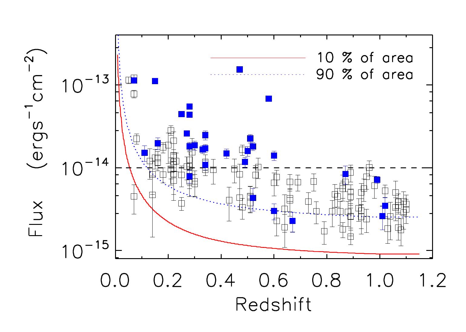
Figure 1: Detected flux (0.5-2 keV band) as a function of redshift for the sample and its modeling. The open black squares with error bars present our identified galaxy groups. The filled blue squares mark the galaxy groups in common with Adami et al. (2011) catalog. Solid red (dotted blue) curve shows the sensitivity achieved at the deepest 10 (90)% area of the survey. The dashed black horizontal line shows the $10^{-14}$ ergs s^-1 cm ^-2 flux threshold adopted for the C1 XMM–LSS sample.

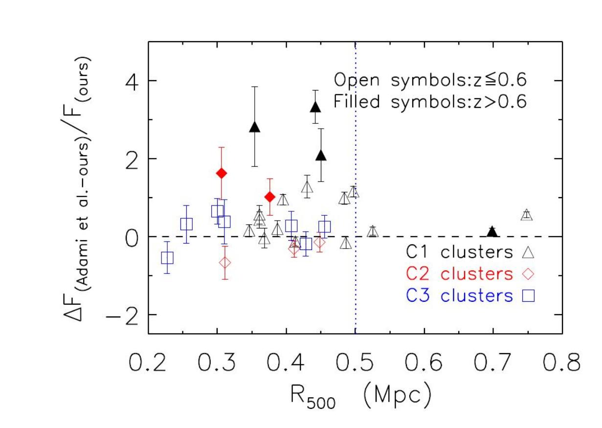
Figure 2: Comparison of the reported flux in the 0.5–2 keV band for galaxy groups and clusters in common between Adami et al. (2011) and our catalog, ($Flux_{(Adami}/Flux_{Ours}-1$) versus $R_{500}$ (Mpc). We illustrate C1 clusters with black triangles, C2 clusters with red diamonds and C3 clusters with blue squares. The filled and open symbols show galaxy groups and clusters at redshift ranges z$>$0.6 and z$\leq$0.6, respectively. The dashed vertical blue line at 0.5 Mpc, marks the fixed radius used for the flux estimates in Adami et al.(2011).

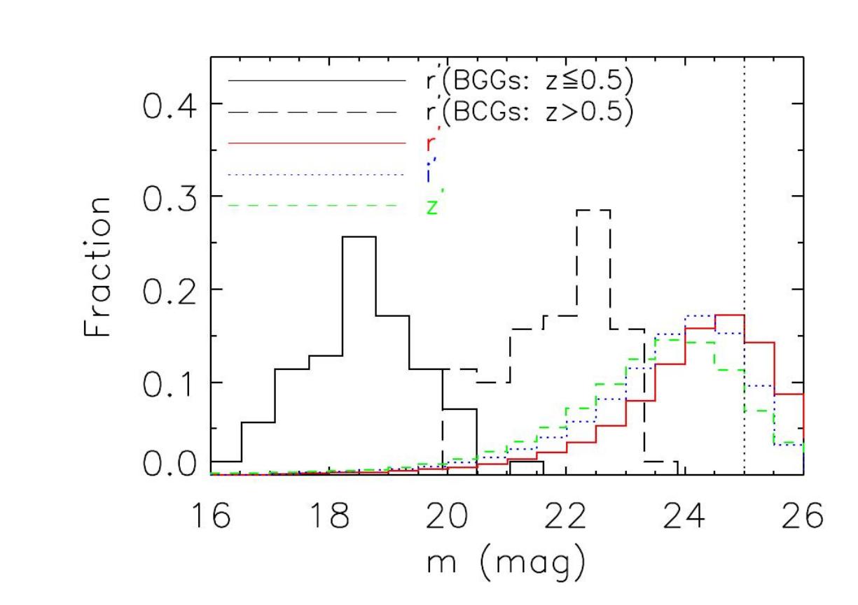
Figure 3: Magnitude distribution of the CFHTLS-W1 photometric data in r^′-, i^′- and z^′ band. The solid and dashed black histograms indicate the r^′-band magnitude distribution of BGGs and BCGs in our catalog in the redshift ranges, z$\leqslant 0.5$ and z$>$0.5, respectively. The dotted black vertical line represents the magnitude completeness of the CFHTLS data in r^′-band.

2.2 Photometric and spectroscopic data

The CFHTLS wide observations have been carried out in the period between 2003 and 2008, covering an effective survey area of $\sim$154 square degrees. The W1 field is the widest field of the CFHTLS survey and covers an area of $\sim$64 square degrees around RA = $02^{h}18^{m}00^{s}$, Dec = $07^{h}00^{m}00^{s}$. The optical images and data of the CFHTLS were obtained with the MegaPrime instrument mounted on the CFHT in the five filters u^∗, g^′, r^′, i^′ and z^′ (e.g., Erben et al. 2013).

The completeness limits and image quality of the photometric survey data are important for the detection of the optical counterparts of the X-ray sources and for the accuracy of the photometric redshift of galaxies (e.g., Mirkazemi et al. 2014; Brimioulle et al. 2008; Bordoloi et al. 2012).

For the purposes of our study the completeness toward the detection of the second brightest galaxies is important for the large magnitude gap systems at high-z.

In Fig. 3 we show the completeness limits, r${}^{\prime}\sim$25 mag (vertical dotted black line), i${}^{\prime}\sim$24.5 mag and z${}^{\prime}\sim$24 mag for the optical data of CFHTLS-W1 field overlapping XMM observations. We also compare the r^′-band magnitude distribution of BGGs in our catalog in two redshift ranges, z$\leq$0.5 (solid black histogram) and z$>$0.5 (dashed black histogram), to the r^′-band completeness limit of the CFHTLS.

This comparison indicates that completeness limit has no effect on the magnitude gap calculation of groups with $\Delta$M${}_{1,2}<$2. However for the z$>0.5$ groups with $\Delta$M${}_{1,2}>2$, the determination of the gap is affected by the completeness. In order to account for this effect in the plots, we assigned all $\Delta$M${}_{1,2}>2$ systems to a single bin (see Fig. 12).

In this paper, we use the photometric redshift catalogs of the CFHTLS survey by Brimioulle et al. (2008); Brimioulle et al. (2013). The XMM-CFHTLS W1 field, has a good spectroscopic coverage of $\sim$ 0.64 degrees² with the VIMOS-VLT Deep Survey (VVDS) (Le Fèvre et al. 2004, 2005) and the targeted cluster follow-up of Adami et al. (2011).

3 Semi-analytic galaxy catalogs

In order to decipher the observational trends it is instructive to compare them to predictions of theory. To this end we have embarked on the semi-analytic galaxy catalogs of B06, DLB07, and G11. All three models implemented on the dark matter halo merging trees obtained from the Millennium simulation which was described in detail in Springel et al. (2005).

The B06 model improves Durham SAMs (GALFORM; e.g., Cole et al. 2000; Benson et al. 2003) notably the black hole growth, AGN feedback (Kauffmann & Haehnelt 2000) and disk instability (Cole et al. 2000; Mo et al. 1998). The DLB07 model is a developed SAM of those presented in Springel et al. (2005), De Lucia et al. (2006) and Croton et al. (2006) models. G11 is an updated version of these models.

To estimate the photometric properties of galaxies, DLB07 and G11 apply the stellar population synthesis model of Bruzual & Charlot (2003) and the initial mass function (IMF) of Chabrier (2003). B06 uses a Kennicutt (1983) IMF with no correction for brown dwarf stars and outputs magnitudes in the Vega system, which we convert to the AB system to match two other models.

G11 refines the definition of a satellite galaxy in halos and treats a galaxy as a satellite, applying the tidal and ram-pressure stripping, only at times when it is located within $R_{vir}$. In two other models a galaxy acts as a satellite when it is ascribed to a larger friends-of-friends halo and its hot gas atmosphere is immediately stripped, leading a reddening in color and a rapid decline in the star formation. Thus, modifications of G11 lead galaxies to retain more gas for star formation.

The merger trees (Harker et al. 2006) used in the B06 model differ from that implemented in DLB07 and G11 (Springel et al. 2005). All three models include star-bursts triggered by major merger, associated with the mass ratio of the merging progenitors in excess of 0.3. When a major merger occurs, all the stellar objects in progenitors are transferred into the bulge of the remnant galaxy. In G11 and DLB07 a fraction of cold gas turns into the bulge stars (Somerville et al. 2001), while in B06 all the cold gas is converted into stars. Among these three models only G11 considers the satellite-satellite mergers, which can reduce the number of satellite galaxies in massive halos (e.g., Kim et al. 2009).

Another relevant physical process for galaxy evolution which has only been taken into account in G11 model is a tidal disruption of the stellar component from merging satellites (e.g., Font et al. 2008; Henriques & Thomas 2010).

Following (e.g., White & Frenk 1991), all three SAMs apply a model for the cooling from hot gas halo. They all define a cooling radius to distinguish between the rapid cooling and static hot halo regimes and compare it with the virial radius (DLB07 and G11) or the free-fall radius (B06). B06 assumes that cooling flows in halos with virial velocities below 50 km s^-1 are suppressed at z$\leq$6 (see B06 and G11). In addition, all the models include the AGN feedback based on the model introduced by Kauffmann & Haehnelt (2000) which suppresses cooling flows in massive halos. The feedback used in B06 is similar to the radio mode feedback considered in Croton et al. (2006), but the details of implementation are different. In B06 AGN feedback is more effective at low-z during the quasi-hydrostatic phase. G11 and DLB07 apply both the radio mode and quasar mode following Croton et al. (2006). In G11 the radio mode feedback and gas cooling are also applied on massive satellite galaxies.

Finally, all three SAMs implement SNe feedback from massive stars, which can heat gas and eject it from the cold disc into the hot halo. G11 uses a model of the SNe feedback which depends on the galaxy circular velocity (V_max) and gives stronger feedback at low-V_max and dwarf galaxies.

In summary, treatments of both minor and major mergers as well as dry and wet mergers, cooling flows, AGN and stellar feedback can affect galaxy evolution and its properties (e.g., stellar mass, luminosity and stellar age). In this paper, we perform a statistical study of the redshift evolution of the magnitude gap out to z=1.1 to compare the galaxy properties in massive halos predicted by different SAMs and examine consistency with observations.

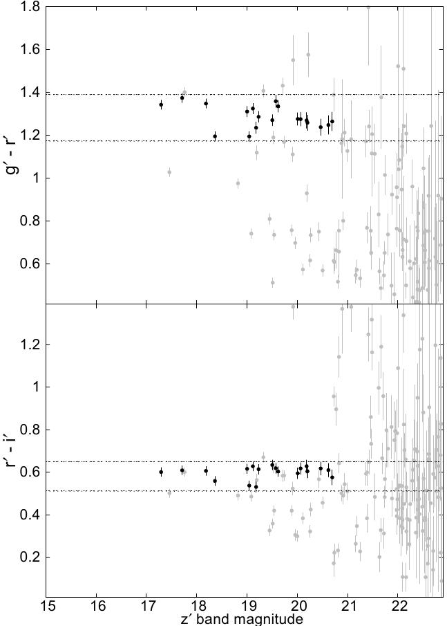
Figure 4: Example of using two color magnitude diagrams to identify the red sequence of a galaxy cluster at z=0.28 (cluster 100320). Top and bottom panels show g^′-r^′ and r^′-i^′ versus z^′-band magnitude, respectively. Gray points are all galaxies within the radius of 0.5 Mpc from the X-ray source center. Black dots are red galaxy group members selected according to the method described in §4.1. The upper and the lower ranges of colors are shown with the horizontal dashed lines.

4 Group Identification

4.1 Red-sequence Method

The full details of our red sequence finder are presented in Mirkazemi et al. (2014), but here we provide an outline of the method. We measure an excess of red sequence galaxies over the background within the 0.5 Mpc radius from the X-ray center. The background is computed using 200 random areas in the CFHTLS survey and repeating the selection of galaxies used in the red sequence. We define the red sequence significance as a ratio of the excess number density of red sequence galaxies to a dispersion in the number density of background galaxies. The redshift at which the red sequence significance reaches its maximum value is taken as the redshift of a cluster. Our red sequence filter is defined as sliding (as a function of redshift) upper and lower limits for galaxy colors and a selection of bright, L$\geq 0.4$ L_∗, galaxies.

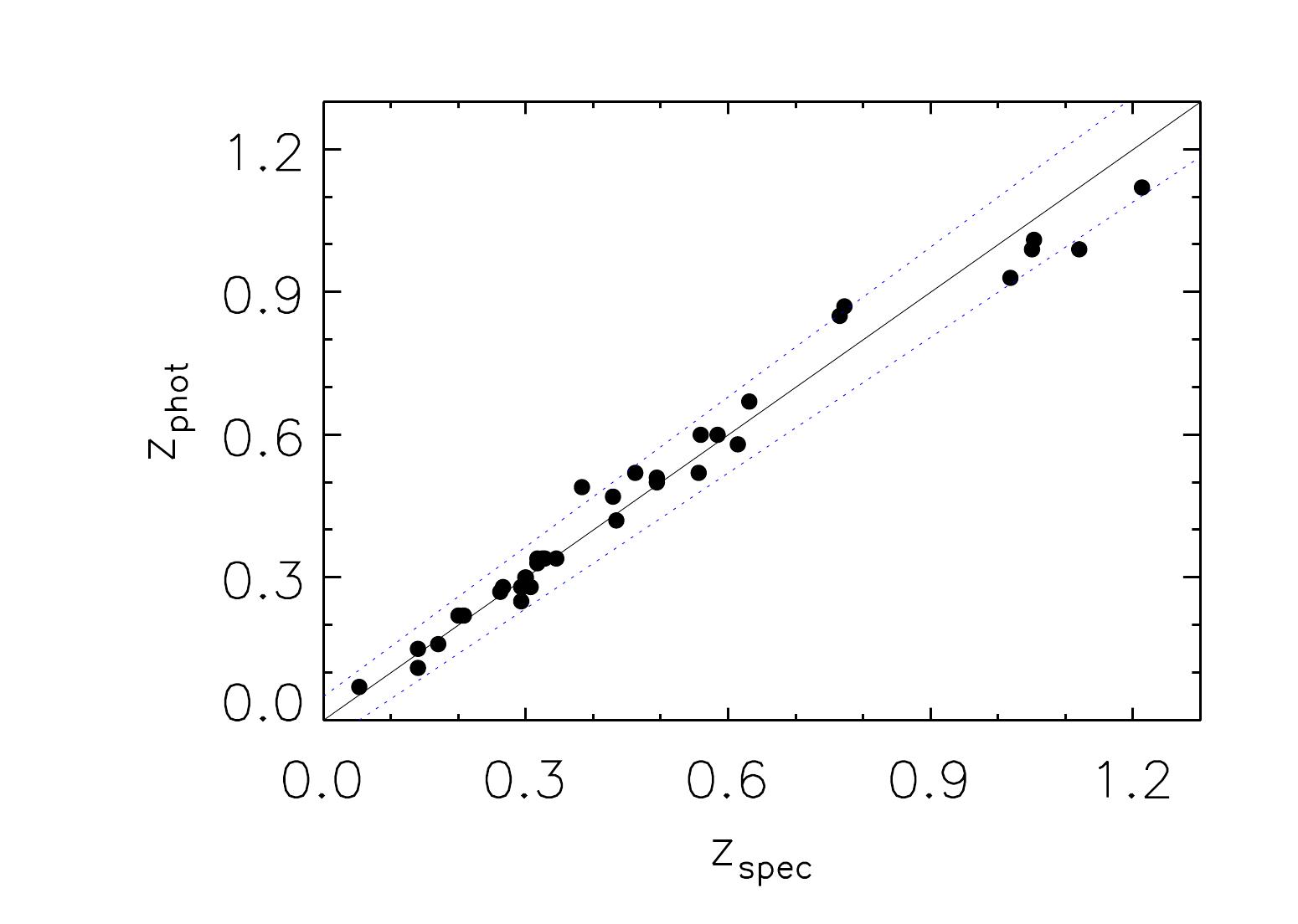
Figure 5: Photometric redshift versus spectroscopic redshift for our sample of galaxy groups. Black line gives the 1:1 relation and the dotted blue lines show the adopted $\pm$0.05(1 + z) uncertainty of our red sequence redshift.

Using Maraston et al. (2009) stellar population models for the red galaxies we derived the characteristic luminosity $L^{\ast}$ for the MegaCam g^′, r^′, i^′ and z^′ filters at each redshift. A model for the colors of red sequence galaxies is derived by a sample of red galaxies with spectroscopic data from the SDSS III (Aihara et al. 2011) and Hectospec (Mirkazemi et al. 2014). This sample of red galaxies gives a model for colors of red galaxies up to a redshift of 0.75. Beyond this redshift, Maraston et al. (2009) stellar population model was used. The upper and lower ranges on colors of red galaxies were defined as $\pm$2$\Delta_{rs}$ around the color model at each redshift. The dispersion $\Delta_{rs}$ has two terms: an intrinsic color dispersion and the measurement uncertainty. The first term is modeled by varying the metallicity in the PEGASE.2 stellar population models (Fioc & Rocca-Volmerange 1999). To compute the second term, we use the error in measuring the magnitudes in the CFHTLS data, as detailed in Bielby et al. (2010).

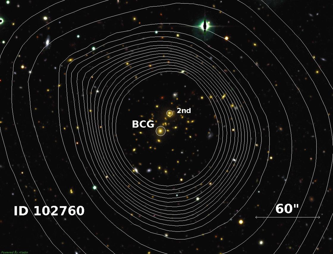
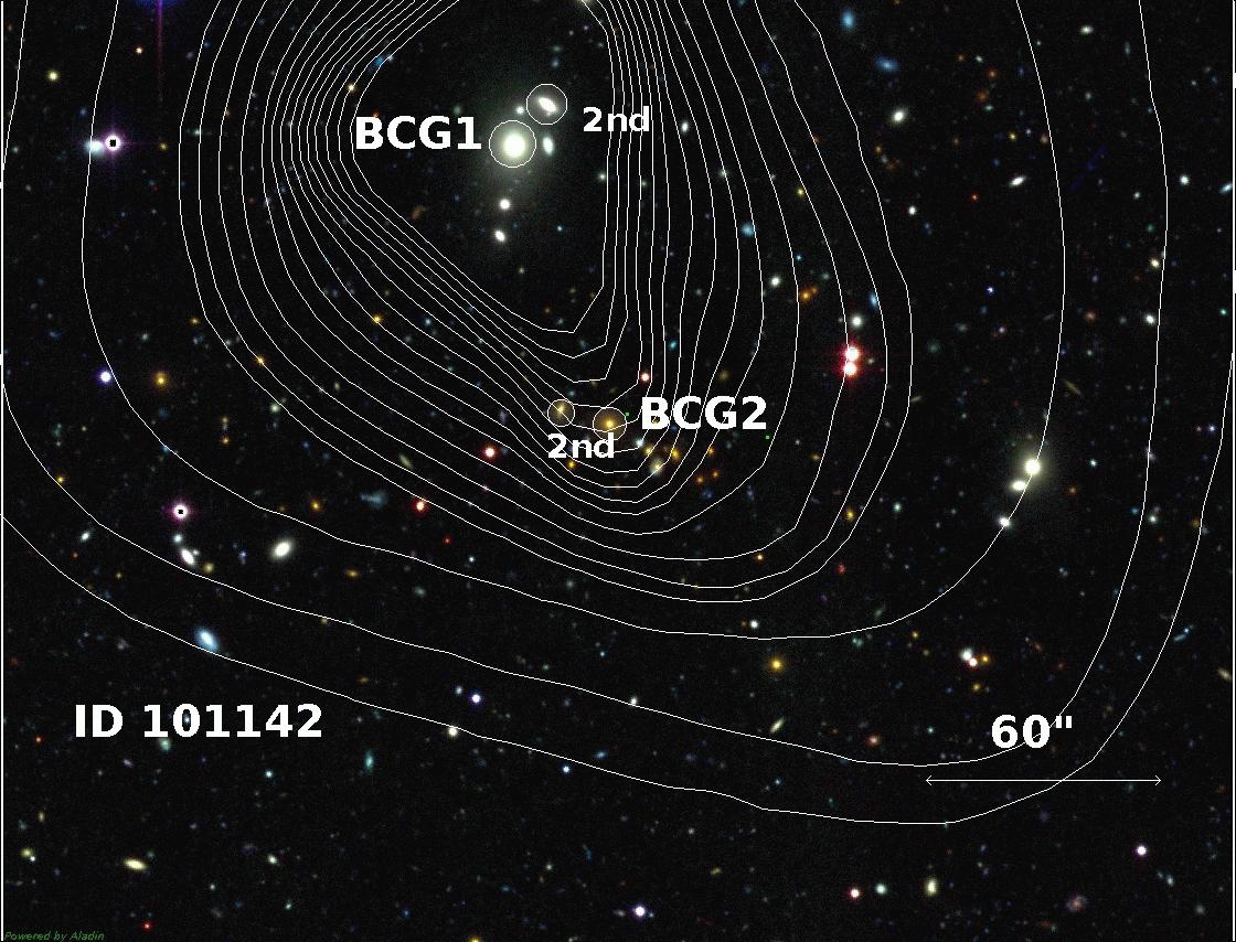
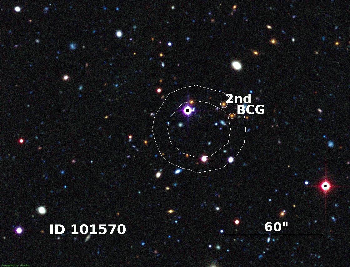
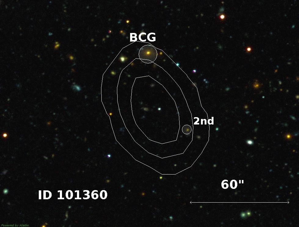
Figure 6: Contours of the extended X-ray emission overlaid on the CFHTLS RGB image in i^′, r^′, g^′ filters. Top left panel shows a spectroscopically confirmed cluster at z=0.47 within the center of X-ray emission and having a single optical counterpart, with a high significance of X-ray flux estimate (flag=1 and flag=3 if without the spectroscopic confirmation). Top right panel, assigned with a flag=2, indicates a presence of two overlapping X-ray sources at z=0.52 and z=0.15. The bottom left image shows the multiple optical counterparts within the X-ray emission with no possibility of separating out their contributions (flag=4). The bottom right panel shows a galaxy group at z=0.60 located at the edge of of X-ray emission (flag=5). The scale bar presented in each image.

We chose the following combination of filters as a function of redshift for the red sequence algorithm:
0.05$\leq$z$\leq$0.66 : g^′, r^′, i^′
0.66$<$z$\leq$1.10 : r^′, i^′, z^′.
Fig. 4 shows the g^′-r^′ and r^′-i^′ colors versus z^′ band magnitude for a cluster at a redshift of 0.28.

For computing the absolute magnitude of red sequence galaxies, we applied a $\chi^{2}$ template-fitting method using the Le Phare package (Arnouts et al. 2002) and templates of Ilbert et al. (2006). We applied the Calzetti et al. (2000) extinction law to the star-forming, irregular and star burst templates. Absolute magnitudes of member galaxies were computed assuming the redshift of their host galaxy group. Similar to Ilbert et al. (2009) and Salvato et al. (2009), we applied the AUTOADAPT mode of the Le Phare code on a sample of galaxies with spectroscopic redshifts from the VVDS survey to reduce the systematic offset between photometric and spectroscopic redshifts by adjusting photometric zero points. Further details of the procedure can be found in Ilbert et al. (2006).

For galaxy groups, located within the VVDS survey, we compute the mean spectroscopic redshift of red sequence galaxies and identify as member the galaxies located within $R_{200}$ from the center of the group and obeying

$$|z_{member}-z_{group}|<3\frac{\sigma_{x}(v)}{c}$$ (1)

We estimate the galaxy velocity dispersion $\sigma_{x}(v)$ using the virial mass of groups (estimated from the X-ray luminosity), as introduced in Erfanianfar et al. (2013). In Tab.1 we present the values of $R_{200}$ and $\sigma_{x}(v)$ for each galaxy group.

We were able to assign a spectroscopic redshift to 15 galaxy groups using the spectroscopic data of the VVDS survey. For further 30 groups and clusters in common with Adami et al. (2011) catalog, spectroscopic redshifts are adopted from that study. For the sample of spectroscopically identified systems, in Fig. 5 we compare the red sequence redshift to the spectroscopic one. The standard deviation between the red sequence and spectroscopic redshifts is 0.04. Black line gives the 1:1 relation and blue dotted lines correspond to the adopted uncertainty in our red sequence redshift determination of $\pm 0.05(1+z)$.

4.2 Visual inspection and identification of group candidates

For identification of galaxy groups, assignment of a photometric redshift and determination of the contamination from several optical groups, we used the red-sequence technique as described in §4.1.

We visually inspected optical counterparts of each X-ray source using the photometric redshift catalog of the CFHTLS (Brimioulle et al. 2008; Brimioulle et al. 2013) and the CFHTLS RGB image in i^′, r^′ and g^′ filters. The visual inspection helps us to assign a redshift to each X-ray source, and to evaluate the correspondence between the galaxy distribution and the X-ray emission. For some sources where we found more than one counterpart and where the shape of X-ray emission allows us to separate the contribution from several counterparts, we specify a new ID in our X-ray source catalog.

We define a flag for each extended X-ray source based on the visual inspection and the position of the over-density of galaxies inside each X-ray source. We use flag values 1 and 3 to mark the best identifications. This requires having both a unique X-ray source with a well-defined center, and a unique optical counterpart with the spectroscopic confirmation for flag=1 or without one – for flag=3. A flag=2 is assigned when a single X-ray source has been split into several sources (e.g., top right panel in Fig.6). A flag=4 indicates a presence of multiple optical counterparts, whose contribution to the observed X-ray emission is not possible to separate or rule out (e.g., bottom left panel in Fig.6).

In cases where the X-ray emission covers a part of the group area and a concentration of galaxies is located at the edge of X-ray emission, we assign a flag=5 (e.g., bottom right panel in Fig 6). Finally, systems with a potentially wrong assignment of optical counterpart are also flagged as 5.

4.3 Catalog of identified groups

We present a catalog of 129 X-ray selected galaxy groups in Tab. 1. Columns 1 and 2 indicate the internal X-ray source ID and our defined group ID. Columns 3 and 4 are the RA (J2000) and Dec (J2000) of the X-ray center. Column 5 shows the group photometric redshift estimated according to the method outlined in §4.1.

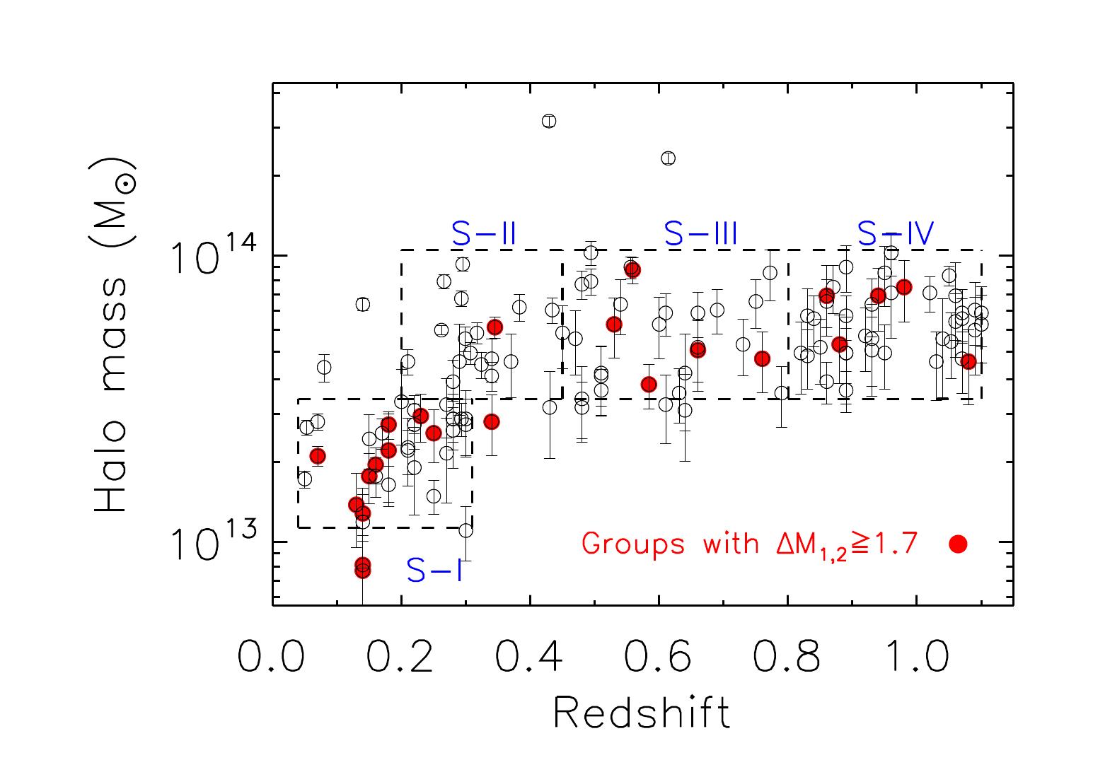
Figure 7: Halo mass versus redshift for the detected X-ray groups. Groups with $\Delta M_{1,2}$$\geq$1.7 have been marked with red filled circles. The dashed boxes show the four subsamples, defined in §4.3.

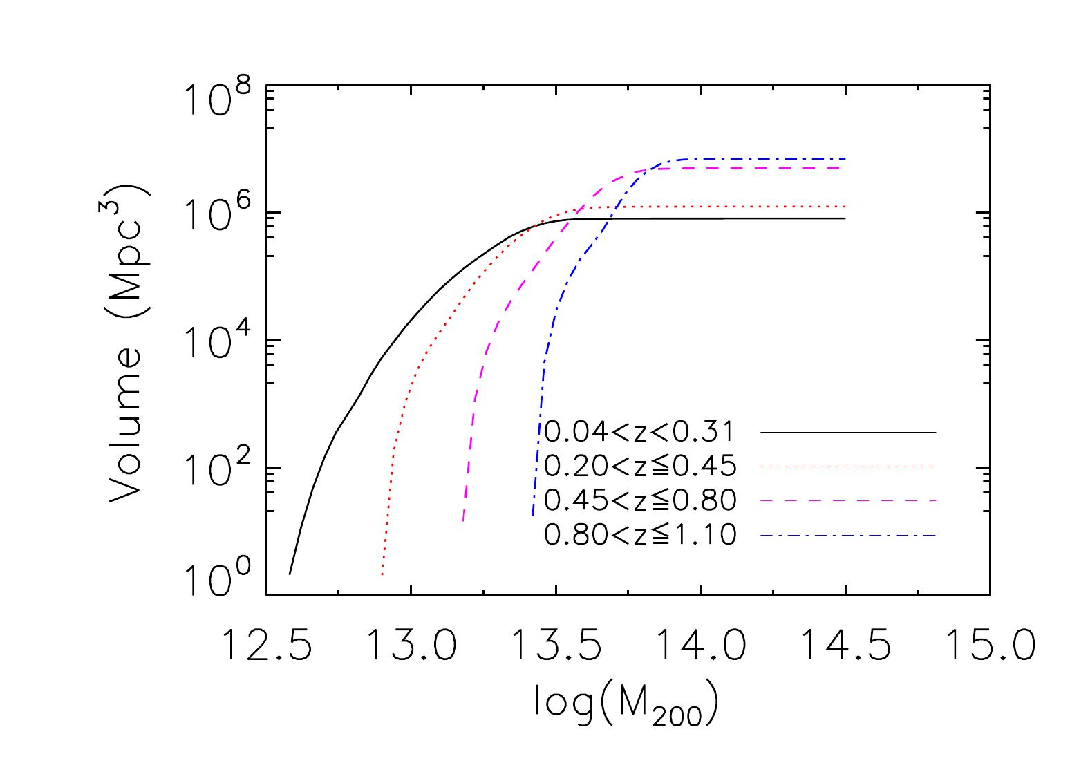
Figure 8: Survey volume as a function of halo mass. Solid black,dotted red, dashed magenta and dashed-dotted blue curves present trends for the four redshift intervals, S-I to S-IV, which are described in §4.3.

Column 6 is the total group mass, $M_{200c}$, in $M_{\odot}$ and a corresponding statistical error, obtained using the $L_{x}-M$ relation of Leauthaud et al. (2010). The systematic uncertainty on inferring $M_{200c}$ using $L_{x}$ is 20% (Allevato et al. 2012). Column 7 lists L_x,0.1-2.4 in the rest-frame 0.1–2.4 keV energy range. Column 8 presents the galaxy velocity dispersion in km s^-1, estimated from $L_{X}$ using the scaling relations (Erfanianfar et al. 2013). Column 9 shows group’s $R_{200c}$ in degrees. Column 10 lists the mean group temperature in keV estimated using L–T relation as in Finoguenov et al. (2007).

The group X-ray flux in the observed 0.5-2 keV band (in units of $10^{-14}$ ergs cm^-2 s${}^{-1})$ and a corresponding $1\sigma$ error is listed in column 11. Column 12 provides the significance of the flux estimate. Column 13 reports the visual flag as defined in §3.1. Column 14 reports the spectroscopic redshift, available for 45 groups. We mark the spectroscopic redshift of groups adopted from with Adami et al. (2011) with ${}^{\prime}*^{\prime}$.

To test the evolution of properties of galaxy groups in observations and SAMs, we define four subsamples using the following redshift and halo mass ranges:

(S–I) 0.0$4<$z$<$0.31 & 13.00$<log(\frac{M_{200}}{M_{\odot}})\leq$13.45

(S–II) 0.20$<$z$\leq$0.45 & 13.45$<log(\frac{M_{200}}{M_{\odot}})\leq$14.02

(S–III) 0.45$<$z$\leq$0.80 & 13.45$<log(\frac{M_{200}}{M_{\odot}})\leq$14.02

(S–IV) 0.80$<$z$\leq$1.10 & 13.45$<log(\frac{M_{200}}{M_{\odot}})\leq$14.02

S–I includes 30 galaxy groups, and other three subsamples, S–II, S–III and S–IV, contain 23, 29 and 41 massive groups, respectively. In Fig. 7, we illustrate subsamples with dashed boxes.

4.4 Abundance of galaxy groups

In order to study the abundance of galaxy groups in our survey, we compute the survey volume using the sensitivity toward the group detection as a function of coordinate in four selected redshift intervals. The components of the calculation consist of the countrate limits as a function of coordinate and a predicted countrate from a galaxy group given its redshift and mass in the $16^{\prime\prime}-128^{\prime\prime}$ aperture defined by the detection scales. The X-ray luminosity of the group is computed for each mass and redshift using the Leauthaud et al. (2010) scaling relation, and the surface brightness profile of the group is computed using the parametrization of Finoguenov et al. (2007). The countrate limits correspond to a four sigma deviation in the background RMS predicted on the scale of the detection, which include the local residual background estimate by the wavelets and the systematic errors on AGN removal. The analysis of the noise of the image on the detection scales has been presented in Connelly et al. (2012) and its negative side is well described by the Gaussian. Fig.8 shows the computed survey volume of the X-ray galaxy groups as a function of the halo mass, M₂₀₀, for different subsamples.

In Fig.9 we compare the number density of galaxy groups as a function of halo mass (solid black histogram with error bar) with that from the SAMs of G11 (red dotted histogram), B06 (dash-dotted blue histogram) and DLB07 (dashed green histogram). Number of observed galaxy groups in each halo mass bin is normalized to the corresponding volume as shown in Fig.8. For the normalization of the number of galaxy groups in the models we use the constant volume of the Millennium simulation, a box of size 500 h^-1Mpc on a side. Halo abundance in models is consistent with the observed trend for S–I (left top panel). For S–II (right top panel ) and S–III (left bottom panel), this consistency becomes worse at high masses, but the agreement reappears at higher redshift traced by the subsample S–IV (right bottom panel).

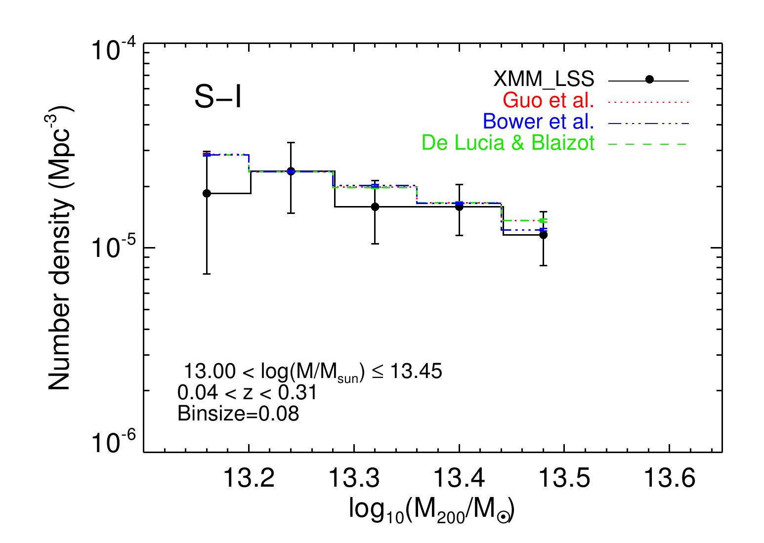
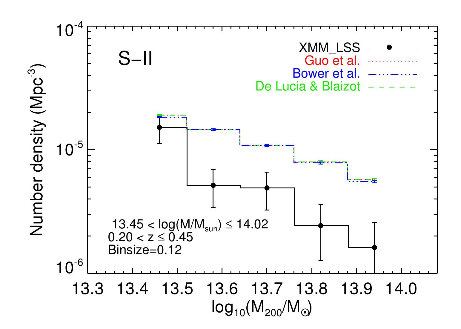
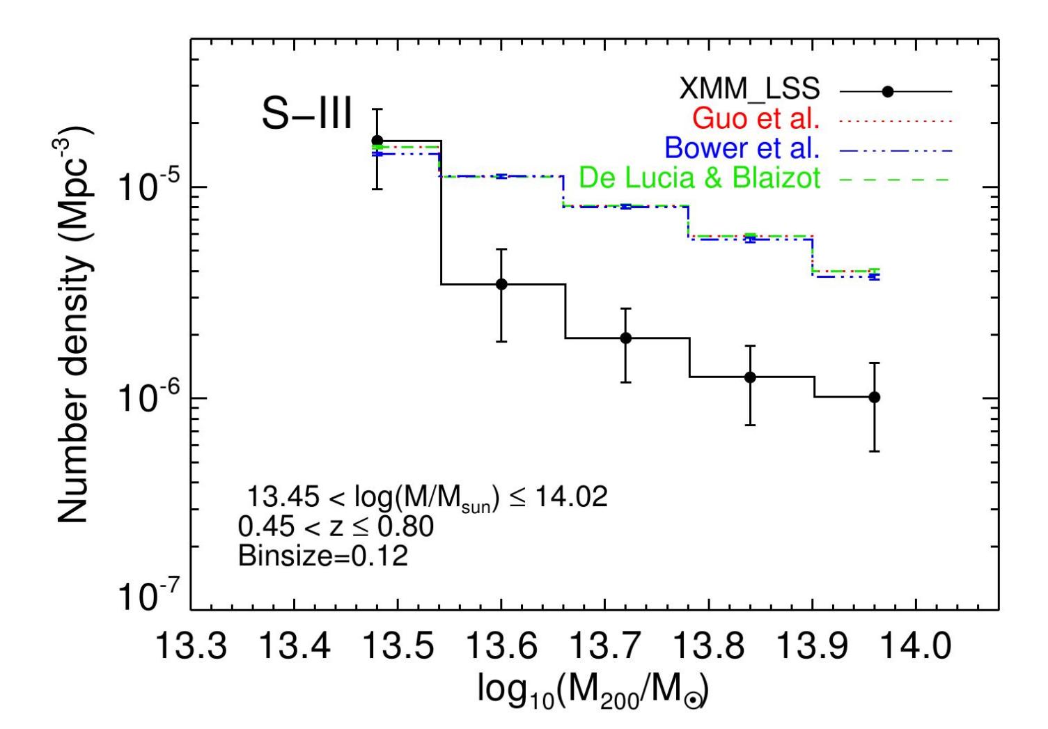
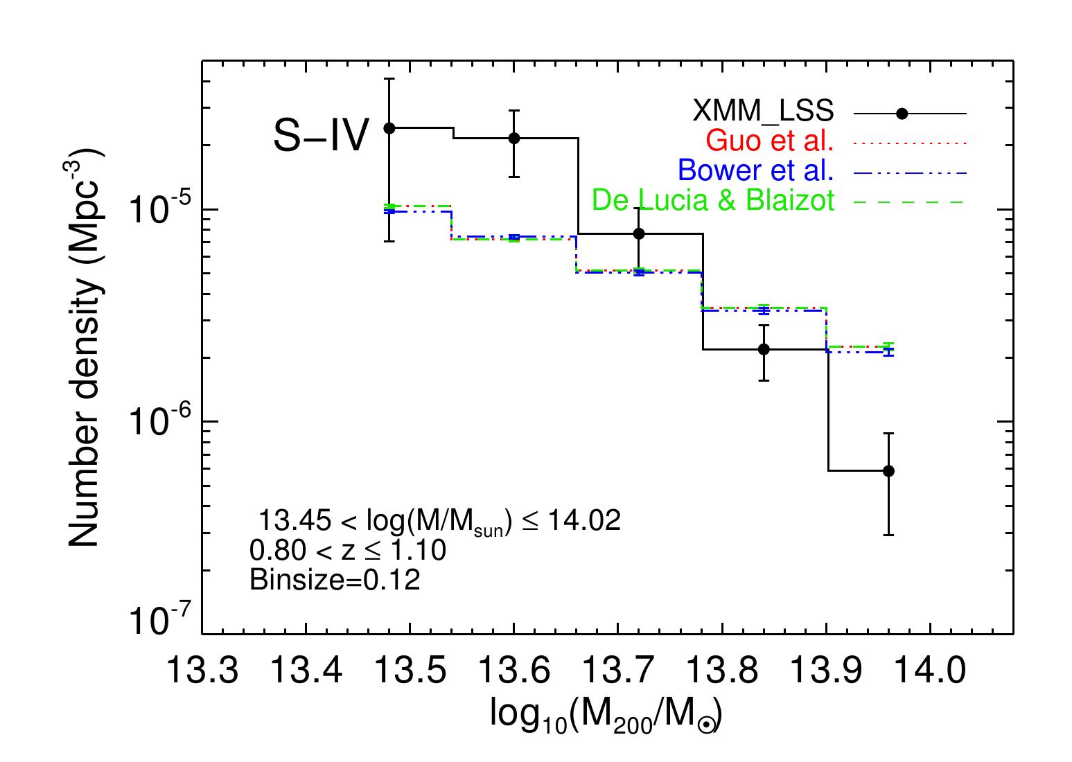
Figure 9: The observed number density of galaxy groups as a function of halo mass (black histogram with error bars) compared to the halo catalogs of B06, DLB07 and G11 for S–I (top left panel), S–II (top right panel), S–III (bottom left panel) and S–IV (bottom right panel). Number density of halos in B06, G11 and DLB07 have been plotted with blue dashed-dotted, red dotted and green dashed histograms and are identical. Halo abundance in simulations is consistent with the observed number density of galaxy groups in S–I, but this consistency is reduced at high masses for S–II and S–III. Subsamples are defined in the legend of each plot.

A detailed assessment of the cosmological importance of the observed halo abundances is outside the scopes of this paper and would need to include the effect of the sample variance at high halo masses. The main conclusion we draw is that for further comparison we should rather use fractions determined separately for the group catalogs in observations and simulations.

5 Membership contamination and magnitude gap calculation

5.1 Contamination of group membership

The purity of the galaxy selection using the red-sequence method is important for calculating the magnitude gap of galaxy groups. In the absence of spectroscopic group membership, the calculation using red sequence galaxies may be contaminated by dusty star forming galaxies (DSFGs).

We examine the impact of contamination of group members by DSFGs using the X-ray galaxy group catalog in the redshift range 0.066$<$z$<$1.544 presented in Erfanianfar et al. (2013) and the data of galaxies in the AEGIS Herschel survey located within a CFHTLS field covering the redshift range 0.05$<$z$<$1.10. We define as DSFGs those galaxies which have star formation rate above $\approx$100 M _⊙ yr^-1 as inferred from FIR observations by Herschel space telescope (Erfanianfar et al. 2014).

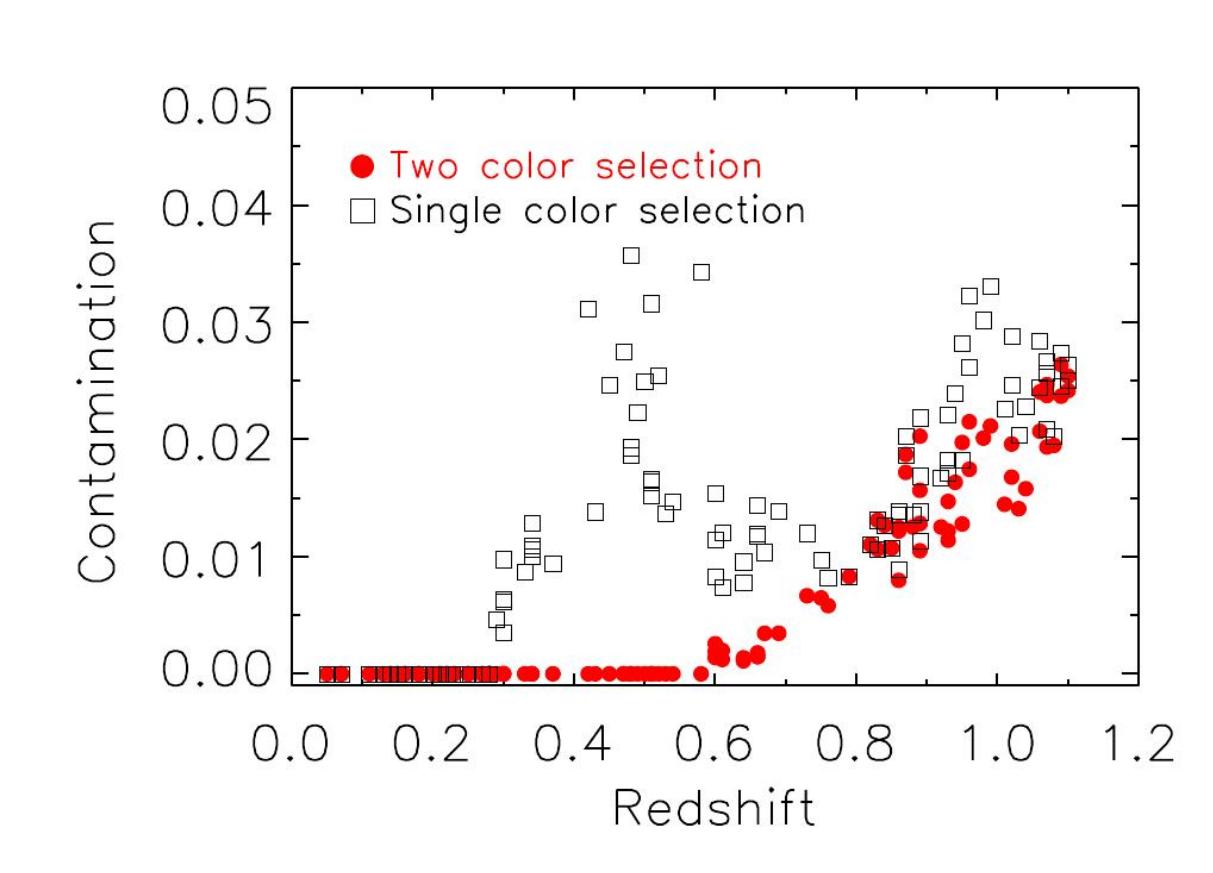
Figure 10: Model prediction for red sequence contamination by dusty star-burst galaxies versus redshift of group. The filled red circles and open black open squares show the contamination for single color and two color selection of group members.

For each group in our CFHTLS catalog we test whether any of DSFGs would be selected as a member. We apply a luminosity cut of L$>$0.4L^∗, and use two red-sequence finders: a single r^′-i^′ color, and our two color selection (§4.1). The contamination for each group is estimated by multiplying the number of DSFGs selected by the red sequence method to the ratio of the area of group which was used to define the magnitude gap (0.5R₂₀₀) and the area of the Herschel data coverage of the AEGIS field, $\sim$0.35 degrees². Fig. 10 shows the expected contamination for each group versus its redshift for the single color and the two color selection of the group members. Two color selection completely removes the contamination at z$<$0.6. The expected contamination by DSFGs at 0.6$<$z$<$1.1 is low, $\lesssim$3%, to significantly affect the magnitude gap measurement.

To examine the effect of the contamination by DSFGs on the magnitude gap calculation, we use data of nine galaxy groups with spectroscopic membership from the AEGIS X-ray groups catalog within the redshift range of 0.65$<$z$<$1.1 (Erfanianfar et al. 2013, 2014). The redshift range of these groups of galaxies covers the range where the contamination by DSFGs is the highest.

Although, the redshifts of these groups do not span the full redshift range of our catalog, they can still give us a good estimate of contamination of the star forming foreground or background galaxies to the red-sequence. For these nine groups, we only find two galaxies as DSFGs which are group members, but they are not selected as a brightest cluster galaxy (BCG) or the second brightest satellite.

Table 1: Catalog of XMM X-ray galaxy groups (for more detail see text in §3.3).

XMM ID	Group ID	RA (J2000)	Dec (J2000)	zphot	$M_{200c}$	$L_{x,(0.1-2.4keV)}$	$\sigma_{v}$	$R_{200}$	kT	Flux	Sig.	Flag	zspec
		degrees	degrees		$10^{13}M_{\odot}$	$10^{42}ergs^{-1}$	kms-1	degree	KeV	$10^{-14}ergs^{-1}cm^{-2}$
(1)	(2)	(3)	(4)	(5)	(6)	(7)	(8)	(9)	(10)	(11)	(12)	(13)	(14)
XMMU J022538.8-050133	100010	36.4119	-5.0261	0.18	3.133 $\pm$0.284	2.41 $\pm$0.35	272.3	0.056	0.8$\pm$0.04	1.757 $\pm$0.255	6.89	3	0.192
XMMU J022330.4-050415	100020	35.877	-5.0708	0.48	3.811 $\pm$0.658	4.875 $\pm$1.38	306.2	0.027	0.98$\pm$0.1	0.334 $\pm$0.094	3.54	5	–
XMMU J022617.1-050447	100030	36.5712	-5.0797	0.07	3.162 $\pm$0.171	2.148 $\pm$0.185	268.6	0.134	0.78$\pm$0.02	12.204 $\pm$1.051	11.61	3	–
XMMU J022402.2-050528	100040	36.0092	-5.0913	0.34	5.248 $\pm$0.439	6.653 $\pm$0.887	332.4	0.04	1.13$\pm$0.06	1.084 $\pm$0.145	7.49	1	0.324*
XMMU J022448.4-050510	100050	36.2019	-5.0863	0.64	3.75 $\pm$0.966	5.998 $\pm$2.588	313.8	0.022	1.02$\pm$0.15	0.191 $\pm$0.082	2.32	5	–
XMMU J022054.0-050610	100060	35.225	-5.1028	0.66	6.237 $\pm$1.161	13.677 $\pm$4.178	373.3	0.026	1.41$\pm$0.16	0.427 $\pm$0.131	3.27	3	–
XMMU J022416.3-050321	100090	36.0682	-5.0559	0.16	2.061 $\pm$0.267	1.222 $\pm$0.256	236.1	0.054	0.64$\pm$0.04	1.158 $\pm$0.242	4.78	3	–
XMMU J022428.9-050545	100100	36.1204	-5.0959	0.51	4.385 $\pm$0.619	6.368 $\pm$1.455	322.8	0.027	1.07$\pm$0.09	0.375 $\pm$0.086	4.37	5	–
XMMU J022846.9-050310	100110	37.1956	-5.0528	0.29	5.37 $\pm$1.503	6.442 $\pm$3.027	331.9	0.045	1.13$\pm$0.19	1.537 $\pm$0.723	2.13	3	–
XMMU J022127.9-050340	100120	35.3663	-5.0613	0.88	6.457 $\pm$1.315	19.907 $\pm$6.683	393.7	0.022	1.56$\pm$0.2	0.294 $\pm$0.099	2.98	5	–
XMMU J022728.1-050319	100130	36.8673	-5.0554	0.13	1.629 $\pm$0.392	0.817 $\pm$0.327	217.2	0.061	0.56$\pm$0.06	1.208 $\pm$0.484	2.49	4	0.143
XMMU J022632.6-050019	100140	36.6359	-5.0055	0.5	10.399 $\pm$0.863	24.155 $\pm$3.206	429.7	0.037	1.86$\pm$0.1	1.59 $\pm$0.211	7.54	1	0.494*
XMMU J022105.9-050012	100150	35.2746	-5.0035	0.16	2.239 $\pm$0.268	1.39 $\pm$0.269	242.6	0.056	0.66$\pm$0.04	1.318 $\pm$0.255	5.17	3	–
XMMU J022628.0-045959	100180	36.6169	-4.9999	0.38	8.492 $\pm$0.718	17.338 $\pm$2.344	400.7	0.035	1.62$\pm$0.09	1.175 $\pm$0.159	7.4	1	0.383*
XMMU J022307.7-045950	100190	35.7821	-4.9974	0.34	4.808 $\pm$0.451	5.794 $\pm$0.871	322.8	0.039	1.07$\pm$0.06	0.945 $\pm$0.142	6.65	3	–
XMMU J022342.5-050203	100200	35.9273	-5.0343	0.89	6.039 $\pm$1.002	18.197 $\pm$4.932	385.8	0.021	1.5$\pm$0.16	0.257 $\pm$0.07	3.69	3	–
XMMU J022609.8-045812	100210	36.5409	-4.97	0.07	3.013 $\pm$0.152	1.991 $\pm$0.159	264.3	0.132	0.76$\pm$0.02	11.337 $\pm$0.904	12.54	1	0.053*
XMMU J022153.1-050132	100220	35.4715	-5.0258	0.27	3.784 $\pm$0.71	3.622 $\pm$1.117	294.3	0.043	0.91$\pm$0.1	1.031 $\pm$0.318	3.24	3	–
XMMU J022740.4-045738	100240	36.9186	-4.9606	0.93	9.057 $\pm$1.556	36.308 $\pm$10.186	444.8	0.023	1.99$\pm$0.22	0.503 $\pm$0.141	3.56	4	–
XMMU J022740.3-045132	100270	36.9181	-4.8591	0.25	8.79 $\pm$0.434	13.183 $\pm$1.03	388.5	0.06	1.52$\pm$0.05	4.444 $\pm$0.347	12.8	1	0.293*
XMMU J022427.8-045014	100300	36.1161	-4.8375	0.48	10.186 $\pm$0.904	22.699 $\pm$3.228	424.9	0.038	1.82$\pm$0.11	1.644 $\pm$0.234	7.03	3	–
XMMU J022803.7-045102	100320	37.0154	-4.8506	0.28	11.535 $\pm$0.514	20.989 $\pm$1.479	427.6	0.06	1.84$\pm$0.05	5.492 $\pm$0.386	14.21	1	0.295*
XMMU J022805.3-045355	100340	37.0222	-4.8988	0.87	10.186 $\pm$1.472	39.995 $\pm$9.397	457.5	0.025	2.1$\pm$0.2	0.675 $\pm$0.159	4.26	3	–
XMMU J022222.7-045314	100370	35.5946	-4.8874	0.37	5.346 $\pm$1.072	7.129 $\pm$2.355	336.1	0.037	1.16$\pm$0.14	0.946 $\pm$0.313	3.03	3	–
XMMU J022500.4-044838	100410	36.2519	-4.8106	0.22	2.259 $\pm$0.575	1.524 $\pm$0.647	245.9	0.043	0.68$\pm$0.09	0.699 $\pm$0.297	2.35	3	–
XMMU J022648.4-044940	100420	36.7019	-4.8279	1.07	5.902 $\pm$1.052	22.699 $\pm$6.637	395.8	0.019	1.58$\pm$0.18	0.19 $\pm$0.056	3.42	5	–
XMMU J022431.6-044815	100430	36.1319	-4.8042	0.98	10.399 $\pm$1.879	48.417 $\pm$14.355	470.2	0.024	2.22$\pm$0.27	0.608 $\pm$0.18	3.37	2	–
XMMU J022236.8-044857	100450	35.6537	-4.816	0.84	7.889 $\pm$1.216	25.704 $\pm$6.457	417.8	0.024	1.76$\pm$0.18	0.449 $\pm$0.113	3.98	5	–
XMMU J022110.4-044206	100480	35.2936	-4.7019	0.75	9.162 $\pm$1.334	28.445 $\pm$6.73	431.7	0.027	1.87$\pm$0.18	0.683 $\pm$0.162	4.23	5	–
XMMU J022525.1-044044	100510	36.3547	-4.679	0.28	10.0 $\pm$0.471	16.788 $\pm$1.25	407.6	0.058	1.67$\pm$0.05	4.364 $\pm$0.325	13.42	1	0.261*
XMMU J022746.4-044523	100520	36.9435	-4.7565	1.04	6.792 $\pm$1.928	27.164 $\pm$12.972	412.7	0.02	1.71$\pm$0.31	0.259 $\pm$0.124	2.09	5	–
XMMU J022422.6-044311	100540	36.0944	-4.7199	0.47	6.561 $\pm$1.303	11.272 $\pm$3.681	366.4	0.033	1.36$\pm$0.17	0.832 $\pm$0.272	3.06	3	–
XMMU J022643.3-044142	100550	36.6805	-4.6952	0.92	7.047 $\pm$1.318	24.21 $\pm$7.43	408.5	0.022	1.68$\pm$0.2	0.325 $\pm$0.1	3.26	1	0.958
XMMU J022222.3-044039	100560	35.593	-4.6777	0.83	8.091 $\pm$1.517	26.363 $\pm$8.110	420.6	0.024	1.78$\pm$0.22	0.479 $\pm$0.148	3.25	4	–
XMMU J022357.3-043526	100570	35.9891	-4.5906	0.51	13.092 $\pm$0.989	35.075 $\pm$4.227	464.6	0.04	2.17$\pm$0.11	2.255 $\pm$0.272	8.3	1	0.494*
XMMU J022438.4-043759	100580	36.1602	-4.6333	0.61	8.241 $\pm$1.072	19.634 $\pm$4.140	405.7	0.03	1.66$\pm$0.14	0.771 $\pm$0.162	4.75	3	–
XMMU J022135.3-044004	100590	35.3973	-4.6679	0.28	3.999 $\pm$0.714	4.009 $\pm$1.175	300.4	0.042	0.94$\pm$0.1	1.044 $\pm$0.306	3.42	5	–
XMMU J022120.6-043729	100600	35.3361	-4.6248	0.14	1.422 $\pm$0.364	0.668 $\pm$0.286	208.0	0.054	0.53$\pm$0.06	0.831 $\pm$0.356	2.34	5	–
XMMU J022830.7-043942	100620	37.1283	-4.6618	0.66	6.039 $\pm$1.312	13.002 $\pm$4.677	369.2	0.026	1.38$\pm$0.19	0.405 $\pm$0.146	2.78	3	–
XMMU J022200.2-043808	100640	35.50081	-4.63559	0.34	3.336 $\pm$ 0.637	3.271$\pm$ 0.102	285.7	0.0341	0.87$\pm$ 0.09	0.534 $\pm$ 0.167	3.18	1	0.317
XMMU J022204.3-043243	100660	35.5179	-4.5453	0.33	6.653 $\pm$0.454	9.484 $\pm$1.033	359.0	0.044	1.31$\pm$0.06	1.665 $\pm$0.181	9.2	1	0.317*
XMMU J022225.5-043741	100690	35.6066	-4.6281	1.1	7.78 $\pm$1.545	36.475 $\pm$11.94	436.5	0.02	1.91$\pm$0.25	0.315 $\pm$0.103	3.06	5	–
Continued on next page

Table 1: Catalog of XMM-CFHTLS X-ray selected galaxy groups, continued from previous page

XMM ID	Group ID	RA(J2000)	Dec (J2000)	zphot	$M_{200c}$	$L_{x,(0.1-2.4keV)}$	$\sigma_{v}$	$R_{200}$	kT	Flux	Sig.	Flag	zspec
		(degrees	(degrees)		$10^{13}M_{\odot}$	$10^{42}ergs^{-1}$	kms-1	degree	KeV	$10^{-14}ergs^{-1}cm^{-2}$
(1)	(2)	(3)	(4)	(5)	(6)	(7)	(8)	(9)	(10)	(11)	(12)	(13)	(14)
XMMU J022700.2-043422	100700	36.751	-4.573	0.05	1.963 $\pm$0.113	0.998 $\pm$0.091	228.4	0.157	0.6$\pm$0.02	11.442 $\pm$1.047	10.93	3	–
XMMU J022303.2-043621	100740	35.7634	-4.6059	1.02	7.834 $\pm$1.23	32.961 $\pm$8.433	431.1	0.021	1.87$\pm$0.19	0.347 $\pm$0.089	3.91	1	1.213*
XMMU J022620.3-043633	100750	36.5849	-4.6092	0.51	4.864 $\pm$1.045	7.465 $\pm$2.655	334.0	0.029	1.14$\pm$0.15	0.442 $\pm$0.157	2.81	5	–
XMMU J022727.0-043223	100760	36.8629	-4.54	0.28	5.715 $\pm$0.406	7.015 $\pm$0.791	338.4	0.048	1.17$\pm$0.05	1.815 $\pm$0.205	8.86	1	0.307*
XMMU J022306.0-043403	100780	35.7751	-4.5677	0.82	6.109 $\pm$1.294	16.711 $\pm$5.861	382.2	0.022	1.47$\pm$0.2	0.298 $\pm$0.104	2.85	5	–
XMMU J022712.9-043536	100792	36.804	-4.5936	0.3	3.334 $\pm$0.687	3.105 $\pm$1.054	283.7	0.038	0.86$\pm$0.1	0.687 $\pm$0.233	2.94	3	0.30
XMMU J022331.5-043439	100810	35.8815	-4.5776	1.07	8.531 $\pm$1.321	40.457 $\pm$10.186	447.7	0.021	2.01$\pm$0.2	0.387 $\pm$0.097	3.97	5	–
XMMU J022148.6-043110	100820	35.4526	-4.5196	0.21	2.582 $\pm$0.368	1.854 $\pm$0.429	256.6	0.047	0.72$\pm$0.05	0.95 $\pm$0.22	4.32	3	–
XMMU J022254.1-043308	100830	35.7255	-4.5524	1.03	5.662 $\pm$1.148	20.137 $\pm$6.730	387.7	0.019	1.52$\pm$0.19	0.184 $\pm$0.062	2.99	5	–
XMMU J022540.0-042841	100860	36.4168	-4.4781	0.22	3.556 $\pm$0.362	3.09 $\pm$0.505	285.9	0.05	0.87$\pm$0.05	1.418 $\pm$0.232	6.11	1	0.203
XMMU J022556.6-042834	100870	36.486	-4.4764	0.89	8.204 $\pm$1.091	29.376 $\pm$6.324	427.4	0.023	1.84$\pm$0.16	0.447 $\pm$0.096	4.65	1	0.979
XMMU J022859.9-042936	100880	37.2499	-4.4935	0.54	8.65 $\pm$1.469	19.143 $\pm$5.321	406.9	0.033	1.67$\pm$0.18	1.022 $\pm$0.284	3.6	5	–
XMMU J022235.9-042854	100910	35.6496	-4.4818	1.08	5.754 $\pm$1.245	22.182 $\pm$7.943	393.4	0.018	1.56$\pm$0.21	0.178 $\pm$0.064	2.79	3	–
XMMU J022132.7-042655	100920	35.3865	-4.4489	0.3	3.184 $\pm$0.59	2.884 $\pm$0.877	279.3	0.037	0.83$\pm$0.09	0.638 $\pm$0.194	3.29	3	–
XMMU J022827.9-042600	100940	37.1163	-4.4335	0.42	8.279 $\pm$0.675	15.066 $\pm$1.963	392.2	0.039	1.55$\pm$0.08	1.489 $\pm$0.194	7.68	1	0.434*
XMMU J022142.0-042739	100950	35.425	-4.4608	0.28	3.062 $\pm$0.65	2.642 $\pm$0.927	274.8	0.039	0.81$\pm$0.09	0.69 $\pm$0.242	2.85	3	–
XMMU J022523.5-042649	100960	36.3482	-4.447	0.52	4.909 $\pm$0.908	7.691 $\pm$2.333	335.7	0.028	1.15$\pm$0.13	0.433 $\pm$0.132	3.29	1	0.462*
XMMU J022610.7-042433	100970	36.545	-4.4094	0.66	8.185 $\pm$1.138	20.941 $\pm$4.721	408.8	0.028	1.68$\pm$0.15	0.676 $\pm$0.152	4.44	3	–
XMMU J022325.6-042721	100980	35.8568	-4.4559	0.61	3.963 $\pm$0.817	6.266 $\pm$2.128	317.9	0.023	1.04$\pm$0.13	0.228 $\pm$0.078	2.94	3	–
XMMU J022332.5-042550	101000	35.8854	-4.4308	0.76	5.728 $\pm$1.04	13.868 $\pm$4.121	369.8	0.023	1.38$\pm$0.16	0.299 $\pm$0.089	3.36	5	–
XMMU J022711.8-425457	101020	36.79945	-4.42938	0.21	1.935$\pm$0.423	1.178 $\pm$ 0.426	233.0	0.042	0.62$\pm$0.07	0.599$\pm$ 0.216	2.76	3	–
XMMU J022433.8-041427	101030	36.1409	-4.2411	0.27	6.871 $\pm$0.195	9.205 $\pm$0.412	359.1	0.052	1.31$\pm$0.02	2.595 $\pm$0.116	22.37	1	0.262*
XMMU J022139.2-042423	101040	35.4136	-4.4066	0.28	3.342 $\pm$0.6	3.027 $\pm$0.891	282.2	0.04	0.85$\pm$0.09	0.79 $\pm$0.233	3.4	4	–
XMMU J022539.8-042255	101060	36.4159	-4.382	0.89	11.995 $\pm$1.687	53.088 $\pm$12.134	484.8	0.026	2.37$\pm$0.22	0.875 $\pm$0.2	4.37	3	–
XMMU J022127.8-042342	101080	35.366	-4.395	1.09	7.396 $\pm$1.675	33.266 $\pm$12.503	428.4	0.02	1.85$\pm$0.27	0.289 $\pm$0.108	2.66	5	–
XMMU J022536.3-042152	101090	36.4013	-4.3645	0.22	2.78 $\pm$0.489	1.928 $\pm$0.555	260.5	0.064	0.74$\pm$0.07	2.117 $\pm$0.609	3.48	1	0.142
XMMU J022208.1-042113	101120	35.534	-4.3536	1.1	8.395 $\pm$1.489	41.115 $\pm$11.967	447.6	0.021	2.01$\pm$0.23	0.364 $\pm$0.106	3.44	3	–
XMMU J022328.3-042132	101130	35.868	-4.3591	0.79	4.315 $\pm$0.794	9.311 $\pm$2.812	338.5	0.02	1.17$\pm$0.13	0.171 $\pm$0.052	3.31	5	–
XMMU J022531.8-041351	101141	36.3825	-4.2311	0.15	8.222 $\pm$0.33	10.495 $\pm$0.667	373.9	0.091	1.41$\pm$0.04	11.144 $\pm$0.707	15.75	1	0.140*
XMMU J022529.0-041540	101142	36.3708	-4.2613	0.52	11.695 $\pm$0.798	29.923 $\pm$3.243	448.5	0.038	2.02$\pm$0.09	1.81 $\pm$0.196	9.21	1	0.556*
XMMU J022506.7-041851	101150	36.2781	-4.3144	0.89	8.892 $\pm$1.186	33.266 $\pm$7.178	438.8	0.024	1.93$\pm$0.17	0.513 $\pm$0.111	4.63	4	–
XMMU J022403.8-041319	101181	36.016	-4.2221	0.99	11.429 $\pm$0.659	56.885 $\pm$5.212	486.2	0.024	2.38$\pm$0.09	0.715 $\pm$0.065	10.92	1	1.050*
XMMU J022406.0-041443	101182	36.0254	-4.2453	0.89	4.487 $\pm$0.551	11.429 $\pm$2.270	349.3	0.019	1.24$\pm$0.09	0.147 $\pm$0.029	5.04	2	–
XMMU J022239.6-041819	101200	35.6651	-4.3055	0.47	4.385 $\pm$0.75	5.998 $\pm$1.679	320.2	0.029	1.06$\pm$0.11	0.436 $\pm$0.122	3.57	3	0.493
XMMU J022519.4-041908	101210	36.331	-4.3191	0.15	2.056 $\pm$0.34	1.205 $\pm$0.326	235.6	0.058	0.63$\pm$0.05	1.318 $\pm$0.356	3.7	3	0.143
XMMU J022220.2-041641	101230	35.5843	-4.2782	0.28	4.487 $\pm$0.689	4.797 $\pm$1.199	312.1	0.044	1.01$\pm$0.09	1.248 $\pm$0.312	4.0	3	–
XMMU J022309.5-041717	101240	35.7899	-4.2883	0.95	6.109 $\pm$1.156	20.23 $\pm$6.295	391.8	0.02	1.55$\pm$0.19	0.24 $\pm$0.075	3.22	3	–
XMMU J022709.6-041810	101250	36.7901	-4.303	1.01	6.683 $\pm$1.297	25.351 $\pm$8.110	408.2	0.02	1.68$\pm$0.21	0.261 $\pm$0.083	3.13	1	1.053*
XMMU J022253.1-041618	101270	35.7213	-4.2718	0.18	1.945 $\pm$0.251	1.146 $\pm$0.238	232.3	0.048	0.62$\pm$0.04	0.828 $\pm$0.172	4.8	3	–
XMMU J022105.7-041831	101280	35.2739	-4.3087	0.93	6.237 $\pm$1.439	20.277 $\pm$7.780	392.9	0.021	1.56$\pm$0.23	0.256 $\pm$0.098	2.61	5	–
XMMU J022643.0-041621	101290	36.6794	-4.2727	0.25	2.951 $\pm$0.506	2.393 $\pm$0.673	270.0	0.042	0.79$\pm$0.07	0.819 $\pm$0.23	3.56	3	–
XMMU J022637.1-041651	101310	36.6548	-4.281	0.93	6.855 $\pm$1.629	23.496 $\pm$9.290	405.4	0.021	1.65$\pm$0.25	0.304 $\pm$0.12	2.53	1	1.018
XMMU J022630.6-041312	101320	36.6278	-4.2201	0.22	3.155 $\pm$0.456	2.559 $\pm$0.603	274.7	0.048	0.81$\pm$0.06	1.179 $\pm$0.277	4.25	1	0.208
Continued on next page

Table 1: Catalogue of XMM-LSS X-ray galaxy groups.

XMM ID	Group ID	RA(J2000)	Dec (J2000)	zphot	$M_{200c}$	$L_{x,(0.1-2.4keV)}$	$\sigma_{v}$	$R_{200}$	kT	Flux	Sig.	Flag	zspec
		(degrees	(degrees)		$10^{13}M_{\odot}$	$10^{42}ergs^{-1}$	kms-1	degree	KeV	$10^{-14}ergs^{-1}cm^{-2}$
(1)	(2)	(3)	(4)	(5)	(6)	(7)	(8)	(9)	(10)	(11)	(12)	(13)	(14)
XMMU J022129.4-041229	101340	35.3727	-4.2082	0.86	9.078 $\pm$1.318	32.961 $\pm$7.762	439.5	0.025	1.94$\pm$0.18	0.559 $\pm$0.132	4.24	3	–
XMMU J022307.4-041309	101350	35.7809	-4.2192	0.67	4.355 $\pm$0.708	7.907 $\pm$2.104	331.8	0.023	1.13$\pm$0.11	0.228 $\pm$0.061	3.76	1	0.631*
XMMU J022725.0-041130	101360	36.8543	-4.1919	0.6	4.592 $\pm$0.627	7.78 $\pm$1.722	333.3	0.025	1.14$\pm$0.09	0.301 $\pm$0.067	4.52	5	0.584*
XMMU J022301.8-040904	101370	35.7578	-4.1511	1.07	8.11 $\pm$1.072	37.411 $\pm$7.998	440.3	0.021	1.95$\pm$0.17	0.351 $\pm$0.075	4.68	2	–
XMMU J022432.2-041001	101380	36.1343	-4.1671	0.25	1.795 $\pm$0.196	1.102 $\pm$0.194	228.8	0.036	0.61$\pm$0.03	0.371 $\pm$0.065	5.68	3	–
XMMU J022447.7-040911	101391	36.1988	-4.1532	0.07	0.953 $\pm$0.21	0.357 $\pm$0.131	181.9	0.047	0.44$\pm$0.04	0.423 $\pm$0.155	2.73	3	0.097
XMMU J022257.6-040709	101400	35.7403	-4.1193	0.28	3.334 $\pm$0.361	3.013 $\pm$0.526	282.6	0.04	0.85$\pm$0.05	0.786 $\pm$0.137	5.73	1	0.293*
XMMU J022419.0-040814	101420	36.0794	-4.1374	0.86	4.797 $\pm$0.605	12.162 $\pm$2.477	355.3	0.02	1.28$\pm$0.1	0.18 $\pm$0.037	4.91	2	–
XMMU J022635.1-040408	101480	36.6465	-4.0691	0.34	7.047 $\pm$0.485	10.52 $\pm$1.151	366.4	0.044	1.36$\pm$0.06	1.716 $\pm$0.188	9.12	1	0.345*
XMMU J022129.7-040543	101490	35.3741	-4.0954	0.94	9.705 $\pm$1.782	40.926 $\pm$12.359	456.0	0.024	2.09$\pm$0.25	0.562 $\pm$0.17	3.31	3	–
XMMU J022201.0-040641	101500	35.5045	-4.1115	0.73	6.471 $\pm$1.096	16.069 $\pm$4.446	383.0	0.024	1.48$\pm$0.16	0.391 $\pm$0.108	3.61	3	–
XMMU J022552.1-040711	101510	36.4675	-4.1199	0.89	6.067 $\pm$1.538	18.365 $\pm$7.745	386.5	0.021	1.51$\pm$0.24	0.26 $\pm$0.11	2.37	5	–
XMMU J022510.0-040148	101530	36.2918	-4.0302	0.16	2.891 $\pm$0.29	2.075 $\pm$0.334	264.3	0.061	0.76$\pm$0.04	1.972 $\pm$0.318	6.21	1	0.17*
XMMU J022529.4-040040	101540	36.3727	-4.0112	0.07	2.366 $\pm$0.159	1.365 $\pm$0.146	243.9	0.121	0.67$\pm$0.02	7.779 $\pm$0.833	9.33	3	–
XMMU J022158.5-040248	101550	35.494	-4.0467	1.06	9.795 $\pm$2.193	49.545 $\pm$18.365	468.0	0.022	2.2$\pm$0.33	0.504 $\pm$0.187	2.69	4	–
XMMU J022702.1-040509	101570	36.7589	-4.0859	0.85	6.281 $\pm$1.227	18.239 $\pm$5.875	387.9	0.022	1.52$\pm$0.19	0.297 $\pm$0.095	3.11	1	0.765
XMMU J022425.6-040057	101580	36.1069	-4.016	1.02	9.84 $\pm$1.045	46.99 $\pm$8.035	465.1	0.023	2.18$\pm$0.15	0.527 $\pm$0.09	5.85	3	–
XMMU J022619.8-040008	101610	36.5827	-4.0024	0.21	5.236 $\pm$0.434	5.585 $\pm$0.738	324.8	0.059	1.09$\pm$0.05	2.827 $\pm$0.374	7.57	3	–
XMMU J022606.9-040315	101620	36.5291	-4.0544	0.2	3.758 $\pm$0.908	3.289 $\pm$1.321	290.3	0.055	0.89$\pm$0.12	1.879 $\pm$0.755	2.49	5	–
XMMU J022222.9-040112	101630	35.5955	-4.02	0.69	8.472 $\pm$1.146	23.014 $\pm$5.058	415.7	0.028	1.74$\pm$0.15	0.67 $\pm$0.147	4.56	3	–
XMMU J022631.6-035640	101720	36.6319	-3.9446	0.34	5.534 $\pm$0.741	7.211 $\pm$1.567	338.2	0.04	1.17$\pm$0.1	1.177 $\pm$0.255	4.61	3	–
XMMU J022406.3-035507	101730	36.0263	-3.9187	0.6	11.535 $\pm$0.94	32.809 $\pm$4.266	453.1	0.034	2.06$\pm$0.11	1.4 $\pm$0.182	7.69	1	0.559*
XMMU J022532.7-035506	101741	36.3864	-3.9184	0.87	11.508 $\pm$1.762	48.417 $\pm$12.078	476.6	0.026	2.29$\pm$0.23	0.839 $\pm$0.209	4.02	1	0.772*
XMMU J022821.2-035223	102090	37.0884	-3.8733	0.28	3.327 $\pm$0.462	2.999 $\pm$0.678	282.4	0.04	0.85$\pm$0.07	0.783 $\pm$0.177	4.43	5	–
XMMU J022229.2-035251	102130	35.622	-3.881	0.23	3.381 $\pm$0.525	2.897 $\pm$0.731	281.7	0.047	0.85$\pm$0.07	1.201 $\pm$0.303	3.96	3	–
XMMU J022303.4-034654	102220	35.7643	-3.7819	0.86	9.506 $\pm$2.0	35.4 $\pm$12.303	446.2	0.025	2.0$\pm$0.28	0.606 $\pm$0.211	2.88	5	–
XMMU J022441.5-034858	102290	36.1732	-3.8163	0.51	4.954 $\pm$0.906	7.674 $\pm$2.307	336.0	0.029	1.16$\pm$0.13	0.455 $\pm$0.137	3.33	3	–
XMMU J022357.5-034311	102570	35.9897	-3.7198	0.95	11.668 $\pm$2.061	55.59 $\pm$16.069	486.0	0.025	2.38$\pm$0.28	0.777 $\pm$0.225	3.46	3	–
XMMU J022644.2-034100	102650	36.6843	-3.6834	0.34	8.872 $\pm$0.693	15.066 $\pm$1.879	395.7	0.047	1.58$\pm$0.08	2.475 $\pm$0.309	8.01	1	0.328*
XMMU J022539.2-034147	102700	36.4133	-3.6966	1.06	7.816 $\pm$1.466	34.834 $\pm$10.715	434.2	0.021	1.89$\pm$0.23	0.332 $\pm$0.102	3.25	3	–
XMMU J022420.5-034135	102750	36.0855	-3.6933	0.64	5.093 $\pm$1.439	9.661 $\pm$4.603	347.5	0.025	1.23$\pm$0.21	0.319 $\pm$0.152	2.1	3	–
XMMU J022145.4-034616	102760	35.4392	-3.7712	0.47	38.019 $\pm$1.164	175.388 $\pm$8.453	658.1	0.06	4.49$\pm$0.1	15.374 $\pm$0.741	20.75	1	0.429*
XMMU J022402.4-034622	102780	36.0103	-3.7728	0.6	7.379 $\pm$1.393	16.331 $\pm$5.058	390.4	0.029	1.54$\pm$0.18	0.659 $\pm$0.204	3.23	3	–
XMMU J022119.1-034451	102810	35.3297	-3.7476	0.43	3.758 $\pm$0.991	4.457 $\pm$1.968	302.1	0.03	0.95$\pm$0.14	0.406 $\pm$0.179	2.27	3	–
XMMU J022752.2-035044	102820	36.9678	-3.8458	0.11	1.517 $\pm$0.203	0.714 $\pm$0.155	211.6	0.069	0.54$\pm$0.03	1.518 $\pm$0.329	4.61	1	0.140*
XMMU J022520.6-034809	102840	36.3359	-3.8026	0.3	6.353 $\pm$0.5	8.472 $\pm$1.064	351.6	0.047	1.26$\pm$0.06	1.864 $\pm$0.234	7.96	1	0.299*
XMMU J022457.1-034905	102900	36.2379	-3.8181	0.58	28.445 $\pm$0.979	130.317 $\pm$7.096	609.7	0.047	3.82$\pm$0.09	6.827 $\pm$0.372	18.38	1	0.614*
XMMU J022246.8-035156	102910	35.6953	-3.8657	0.08	5.07 $\pm$0.452	5.445 $\pm$0.778	322.4	0.054	1.07$\pm$0.06	2.238 $\pm$0.319	7.01	3	–
XMMU J022242.9-035529	102951	35.6789	-3.9249	1.09	8.71 $\pm$1.6	42.954 $\pm$12.942	452.4	0.021	2.06$\pm$0.25	0.393 $\pm$0.119	3.31	3	–
XMMU J022225.2-035701	103010	35.605	-3.9504	0.21	2.618 $\pm$0.57	1.888 $\pm$0.682	257.7	0.047	0.73$\pm$0.08	0.969 $\pm$0.35	2.77	5	–
XMMU J022623.7-034309	103320	36.5988	-3.7194	0.53	7.413 $\pm$1.358	14.825 $\pm$4.457	385.8	0.032	1.5$\pm$0.17	0.817 $\pm$0.246	3.33	3	0.558
XMMU J022134.7-040350	103330	35.3946	-4.0641	0.14	1.012 $\pm$0.404	0.392 $\pm$0.270	185.6	0.048	0.45$\pm$0.07	0.47 $\pm$0.324	1.45	3	–
XMMU J022358.4-045607	103340	35.9936	-4.9355	0.96	13.583 $\pm$1.742	71.285 $\pm$14.791	512.0	0.026	2.65$\pm$0.23	1.006 $\pm$0.209	4.82	5	–

Thus, in this test we also find that the contamination by DSFGs has no effect on the magnitude gap estimate. In addition, one way to inspect the effect of the red sequence selection on the magnitude gap estimate is to compare values of the magnitude gap which are calculated using the photometric membership to that of the spectroscopic membership.

We use the X-ray group catalogs from the AEGIS field (Erfanianfar et al. 2013), the COSMOS field (Finoguenov et al. 2007; George et al. 2011), including all spectroscopic observations, available within the collaboration. We also use all spectroscopic data of groups in our catalog provided by the VVDS data and Adami et al. (2011).

We only consider the $\sim$1 degree² area of the COSMOS survey, that is in common with CFHTLS survey, where a comparison to our red sequence selection using CFHT colors is possible. Altogether, we obtain a catalog of 84 galaxy groups (42 groups from the COSMOS catalog, 26 groups from our catalog and 16 galaxy groups from the AEGIS catalog), having the spectroscopic confirmation of the magnitude gap. These groups span a redshift range of 0.05$<$z$<$1.22, which is similar to the redshift range of our XMM-LSS catalog.

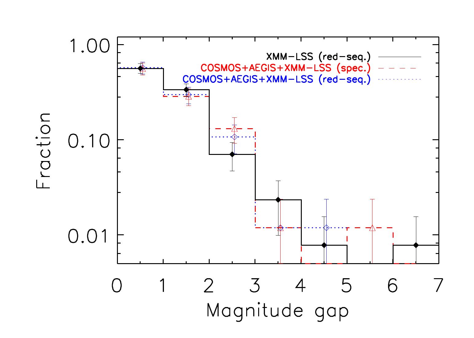
Figure 11: Comparison of the magnitude gap distributions between our X-ray group catalog (XMM-LSS) with the red sequence membership (solid black histogram) and 84 X-ray galaxy groups from the COSMOS+AEGIS+XMM-LSS with the spectroscopic membership (dashed red histogram) and the red sequence membership (dotted blue histogram). The redshift range is 0.05$<$z$<$1.22. A good agreement is seen between the two distributions, implying that the results obtained with the red sequence selection are robust.

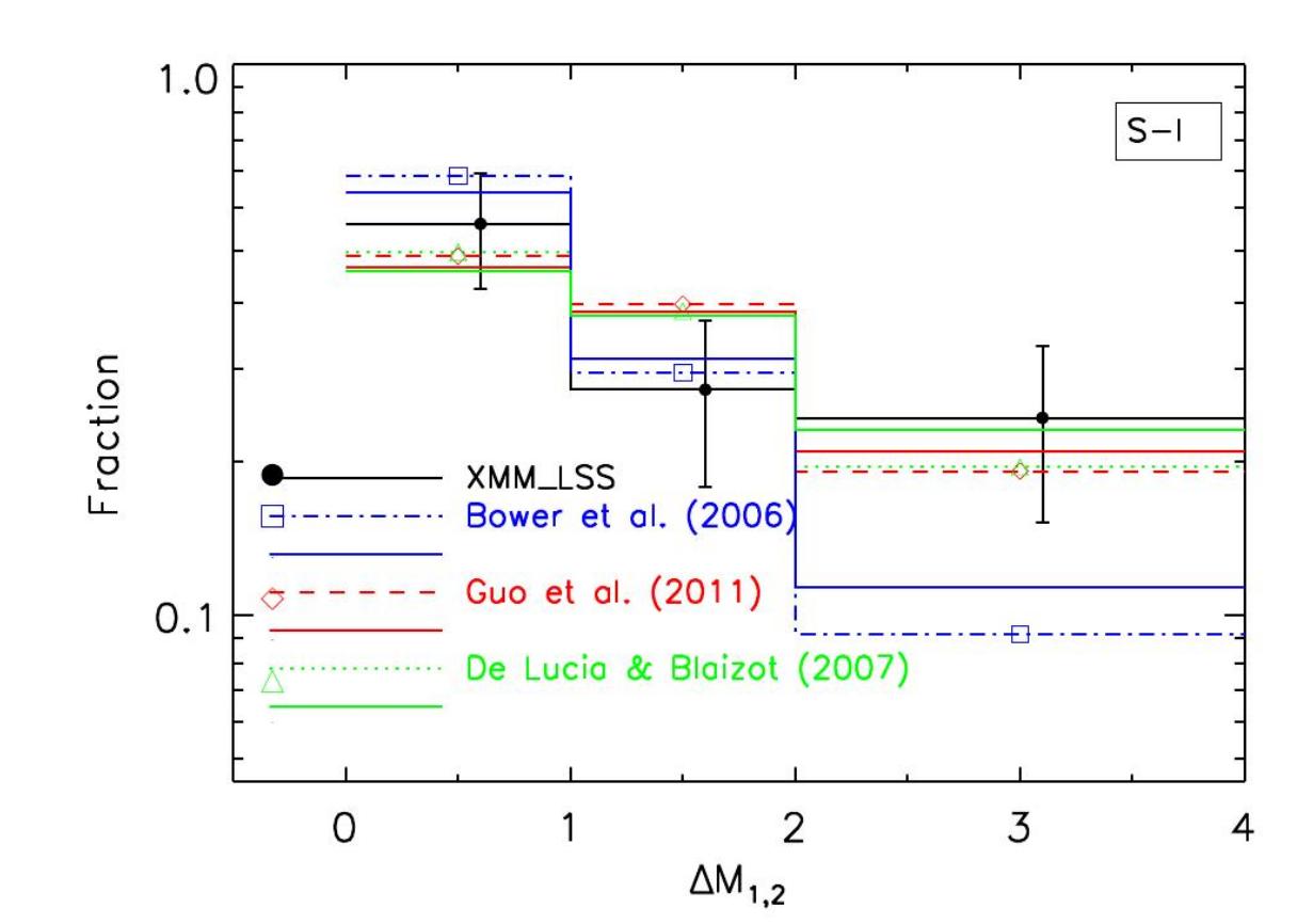
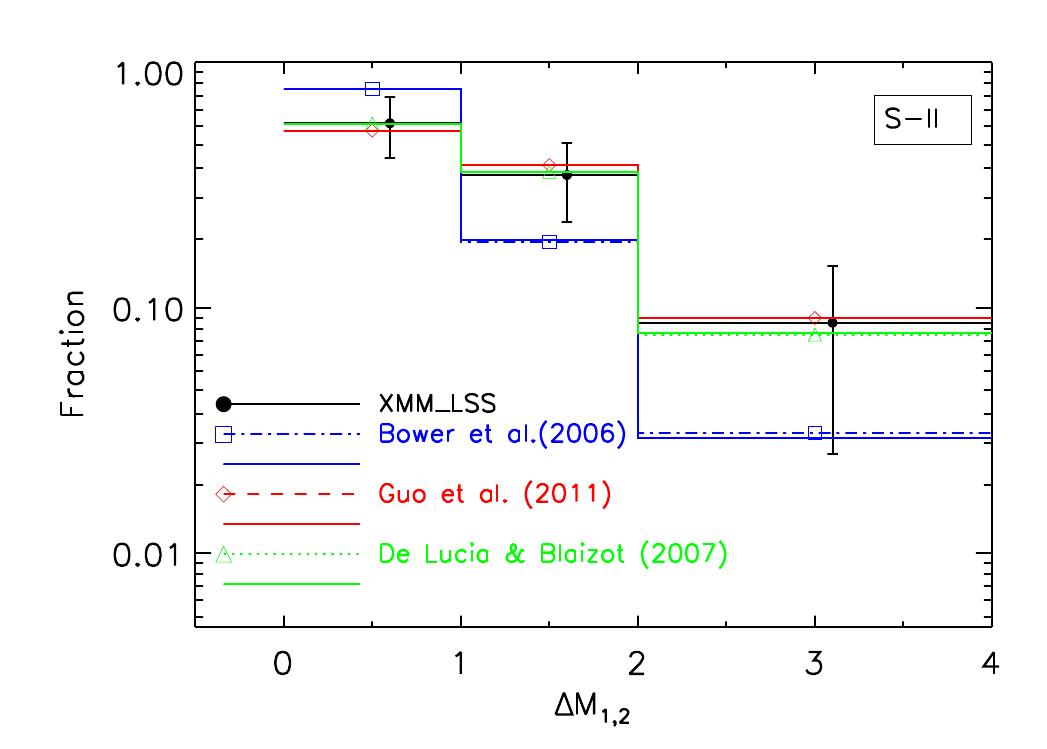
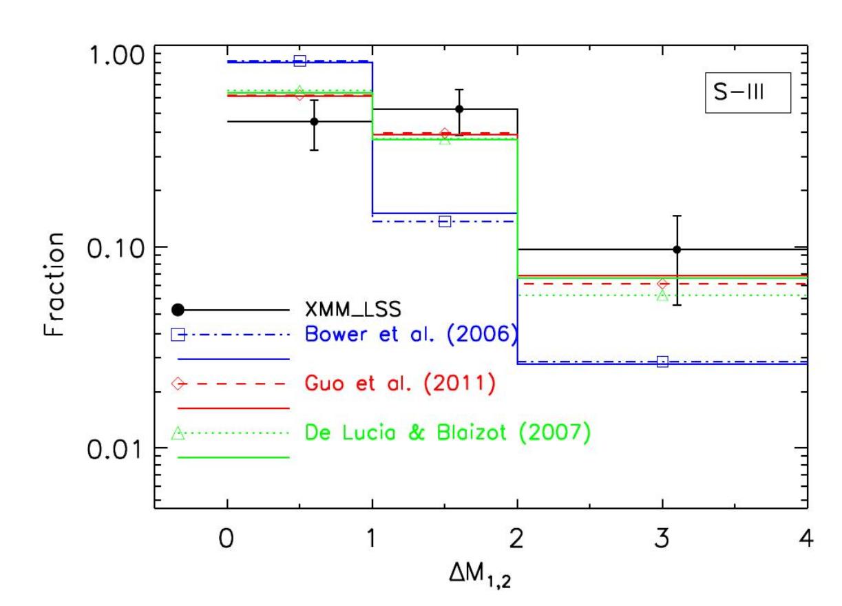
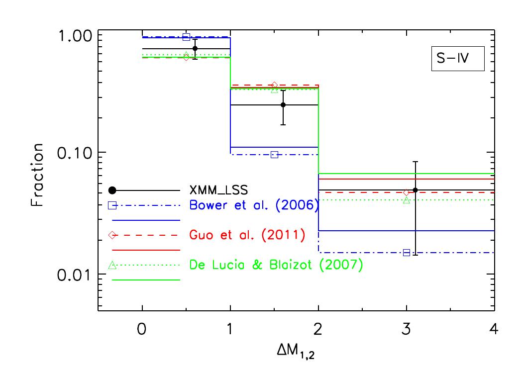
Figure 12: The observed fraction of galaxy groups as a function of their magnitude gap (black points with error bars) compared to the predictions of semi-analytic galaxy formation models, B06 (solid and dashed-dotted blue histograms), DLB07 (solid and dotted green histograms) and G11 (solid and dashed red histograms) for S–I (top left panel), S–II (top right panel), S–III (bottom left panel) and S–IV (bottom right panel). We find that the fraction of groups declines with magnitude gap at all redshifts. Magnitude gap bin sizes are equal to one magnitude for $\Delta M_{1,2}<$2. $\Delta M_{1,2}\geq$2 systems are plotted as a 2 magnitude wide bin.

For this sample of 84 groups (COSMOS+AEGIS+XMM-LSS) we select the red sequence and spectroscopic members of groups according to the approach described in §4.1. We compute the magnitude gap between the first and the second brightest group galaxies using both spectroscopic and photometric group members, separately. The magnitude gaps of the spectroscopic sample range from 0.02 to 5.75.

In Fig.11 we compare the magnitude gap distribution of the COSMOS+AEGIS+XMM-LSS groups for two calculations of gap, one – using red sequence membership (dotted blue histogram) and the other – using the spectroscopic membership (dashed red histogram). It appears that the two distributions do not deviate considerably. In Fig.11 we also compare these distributions to that of our XMM-LSS galaxy groups catalog with red sequence members (solid black histogram).

By comparing the spectroscopic and photometric membership assignment for the COSMOS+AEGIS+XMM-LSS groups, we find that redshifts of the second ranked red sequence galaxies in six groups deviates from the redshift of the hosting galaxy group. The magnitude gaps of these contaminated groups, which have been computed using red sequence galaxies range as follows: three galaxy groups with $\Delta M_{1,2}\geq$1.7 (classified as fossils) and three galaxy groups with $\Delta M_{1,2}\leq$1.28 (classified as non-fossils). Differences between the gap values in two calculations range from 0.05 to 1.2 mag. These deviations do not affect the classification by $\Delta M_{1,2}$ in 5 out of 6 cases. From finding one system to change the classification, we place a 95% confidence limit on the effect of $<6$%, based on the Poisson PDF. We added the uncertainty associated with this to each magnitude bin. Fractionally the effect is strongest for the bin containing the large magnitude gap systems.

5.2 Determination of $\Delta M_{1,2}$ and definition of fossil groups

In a number of studies different fossil group criteria for the magnitude gap and search radius have been used. For instance, La Barbera et al. (2012) defined as fossil groups those elliptical galaxies with no satellite brighter than a given magnitude gap of $\Delta M_{1,2}\geq$1.75, within a search radius of 0.35 Mpc and a maximum redshift difference of 0.001. Voevodkin et al. (2010) classified an object as a fossil group if $\Delta$M${}_{1,2}\geq 1.7$ for galaxies inside 0.7r₅₀₀. Smith et al. (2010) used a fixed projected physical radius of R = 640 kpc ($\sim$ 0.4r₂₀₀) for a sample of massive clusters at z$\sim$0.2 to study the distribution of luminosity gap.

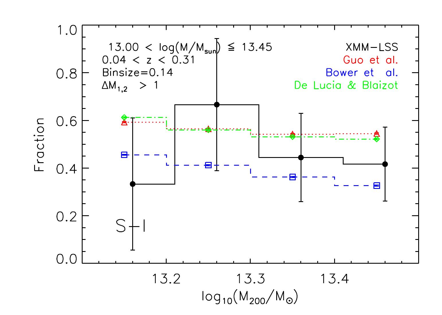
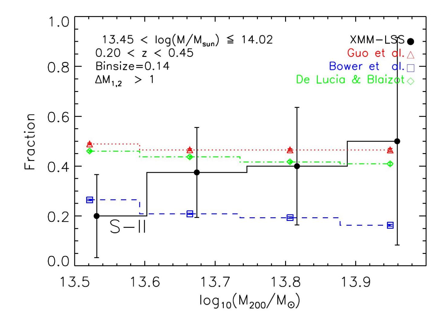
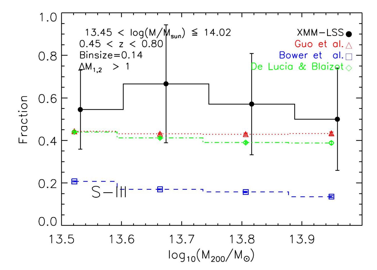
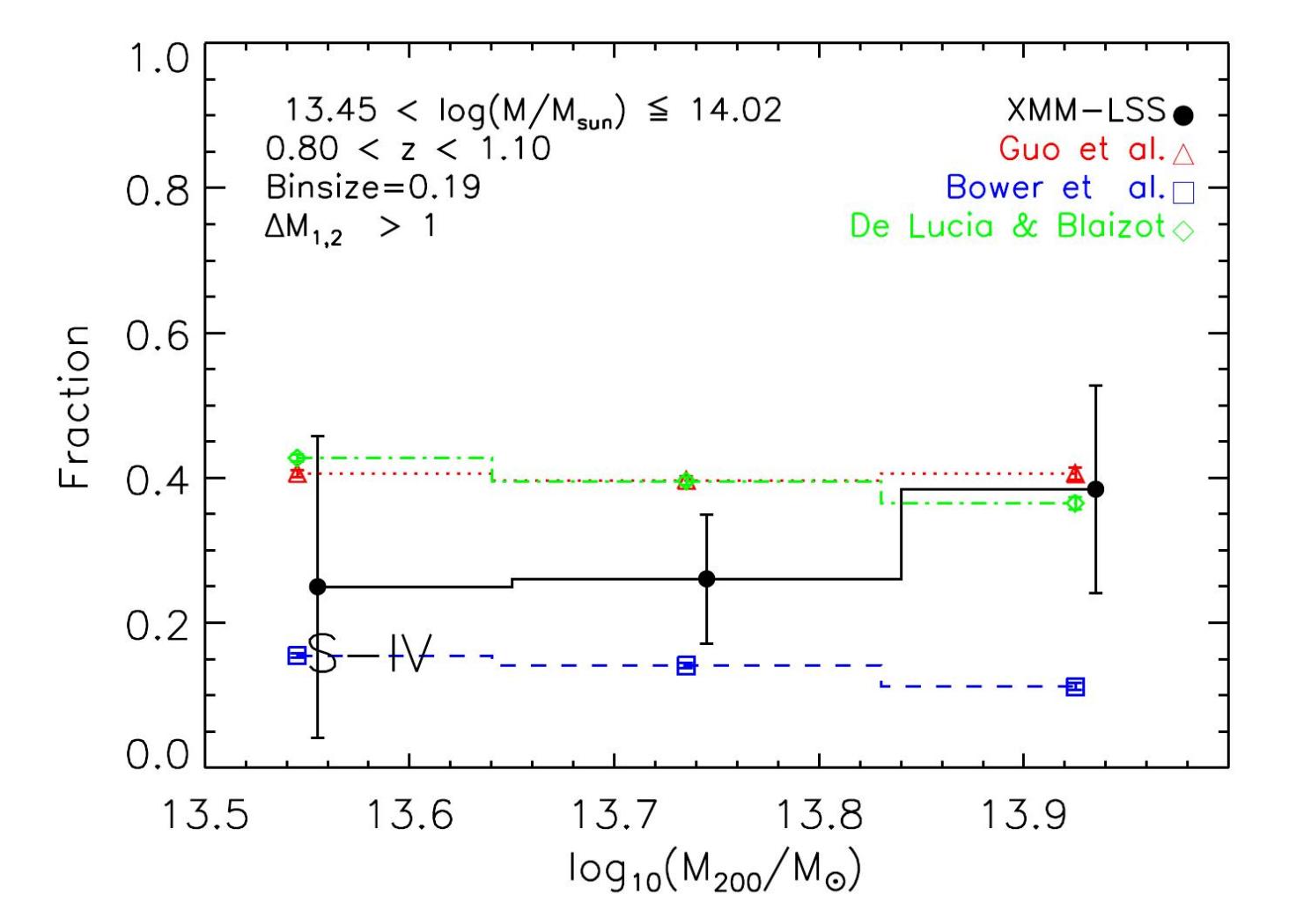
Figure 13: Halo mass dependence of the fraction of groups with $\Delta M_{1,2}>$1. Black points with error bars show the data and dotted red, dashed blue and dash-dotted green histograms present model predictions of G11, B06 and DLB07, respectively for S–I (top left panel), S–II (top right panel), S–III (bottom left panel) and S–IV (bottom right panel). While the data are in agreement with the models, the low statistics of the data prevents us from choosing the best model.

We define the spatial selection of galaxies for the $\Delta M_{1,2}$ calculation in such a way that it allows us to select a subsample of fossil groups candidates. For computing the magnitude gap of a galaxy group, we adopt the coordinates of the BGG as a center of group and measure the magnitude gap, $\Delta M_{1,2}$, using the rest frame absolute r-band magnitude of galaxies between the BGG and the second brightest galaxy within 0.5R₂₀₀, following Jones et al. (2003). The same definition of the magnitude gap has been applied to the SAM catalogs.

We define as a fossil group candidate, the X-ray group of galaxies that has a magnitude gap exceeding $\Delta M_{1,2}\approx$1.7 mag within 0.5R₂₀₀. The low $L_{x}$ cut has been historically done to avoid inclusion of X-ray emitting galaxies. However, by implying this cut one restricts the studies only to massive groups. Since we remove the galactic contribution to the X-ray emission by using only large spatial scales in the flux estimates, we do not have to limit the selection of fossil groups. Our lowest $L_{x}$ group has a luminosity in the rest-frame 0.1–2.4 keV band of (3.6$\pm$1.3)$\times$10⁴¹ ergs s^-1.

6 Results and discussion

6.1 Magnitude gap distribution

We calculate the magnitude gap between the first and the second brightest galaxies in groups and clusters according to the method described in §5.2. For 26 groups in our catalog we calculate the magnitude gap using a spectroscopic membership assignment and for the remaining 102 groups the gaps are calculated using the red-sequence membership assignment.

In Fig.12, we compare the distribution of the magnitude gap between X-ray groups and the predictions of SAMs, G11 , DLB07 and B06. As discussed in §2.2, the completeness limit may affect the magnitude gap calculation of groups with $\Delta$ M${}_{1,2}>$ 2 at z$>$0.5. To account for this effect we define two different bin sizes, with 1 mag for systems with $\Delta M_{1,2}<$2, while assigning all $\Delta M_{1,2}\geq$2 groups to a single bin (see Fig.3). Such a binning scheme is introduced to remove the effect of completeness on the binned fractions.

For SAMs we use both the formal selection of the subsamples (solid histograms) and modeling of the X-ray selection. For the later, we introduce mass-dependent weights, $\frac{V_{obs}(M_{200},z)}{V_{sim}}$. V_obs is the survey volume for detecting groups as a function of $M_{200}$ and z, where V_sim is equal to the (500 Mpc h${}^{-1})^{3}$ volume of the Millennium simulation. We evaluate the total number of groups corresponding to each $\Delta M_{1,2}$ bin by summation of the weighted number of groups. We illustrate the so constructed model magnitude gap distributions with dashed red (G11), dashed-dotted blue (B06) and dotted green (DBL07) histograms in Fig. 12. It can be seen that the differences in the resulting magnitude gap distributions are small compared to our observational errors.

In agreement with the findings of Smith et al. (2010), the fraction of detected groups, $f(\Delta M_{1,2})$, in all histograms of Fig. 12 declines with $\Delta M_{1,2}$. A linear relation provides a good fit to the data. We provide the fit parameters corresponding to each subsample in Tab.2. The slope of the relation is shallower for (S–I) compared to other subsamples, indicating a larger contribution of fossil groups. The trends seen in the data for groups and clusters with $\Delta M_{1,2}\leqslant$3 are well reproduced by both DLB07 and G11 models, while the B06 model predicts the slopes that are too steep. In addition, as previously noticed by Dariush et al. (2010), the B06 model over-predicts the fraction of clusters with $\Delta M_{1,2}\leqslant$1 for S-II to S-IV.

Table 2: Parameters of the linear fit to a distribution of groups over the value of magnitude gap, $\Delta M_{1,2}$.

Subsample	Intercept	slope
S–I	$0.51\pm 0.12$	$-0.11\pm 0.06$
S–II	$0.70\pm 0.01$	$-0.22\pm 0.01$
S–III	$0.57\pm 0.14$	$-0.14\pm 0.07$
S–IV	$0.75\pm 0.17$	$-0.25\pm 0.09$

In Fig. 13, we investigate a mass dependence of the fraction of groups characterized by a large magnitude gap ($\Delta M_{1,2}\geq 1$). The relation reveals a mild dependence on mass, justifying our use of wide mass bins.

Fig. 14 summarizes the trends presented in Fig. 13 and shows the redshift evolution of the mean fraction of large magnitude gap groups/clusters, n(z). We find that n(z) evolves slowly with redshift: n(z)=0.47-0.12$\times$z, in agreement with all models. B06 underestimates fraction of clusters having a large magnitude gap.

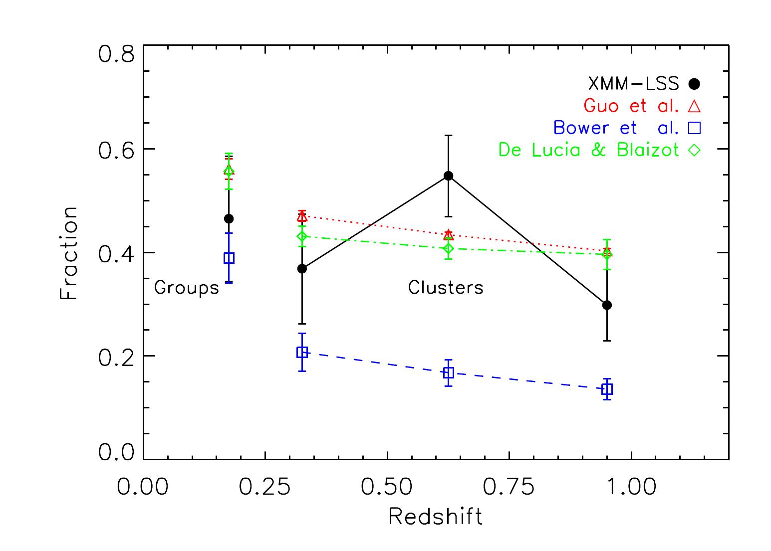
Figure 14: The redshift evolution of the fraction of groups and clusters with $\Delta M_{1,2}>1$. The error bars correspond to the 95% confidence limits of the standard error of the mean.

Behavior of the luminosity gap in groups and clusters can depend on several effects, which we describe below. If a galaxy brighter than the second brightest galaxy falls into the cluster or group, the luminosity gap of the system changes to a lower value, as soon as the infalling galaxy passes into $(0.5R_{200})$, within which the $\Delta M_{1,2}$ is calculated. For the galaxy group members, the dynamical friction causes satellite galaxies to merge together or with the central galaxy. Mergers between satellites can reduce the number of satellite galaxies in SAMs and in massive halos, especially reducing the number of the low-luminosity satellite galaxies; the product of merger is more luminous and massive. Finally, evolution of galaxy properties, most notably the stellar mass and age of the stellar population in both central and satellite galaxies also affects the magnitude gap. This in turn depends on the gas cooling rate, tidal stripping and disruption, AGN and SNe feedback.

The G11 model shows the best agreement with our observational results, possibly due to its advances in modeling the satellite disruption and gas striping due to the tidal and ram-pressure forces and the satellite-satellite merger. These processes are not taken into account in B06 and DLB07, but play an important role in the evolution of the galaxy luminosity in massive halos (Conroy et al. 2007a, b; Henriques & Thomas 2010; Liu et al. 2010).

6.2 Magnitude gap and BCG luminosity relation

6.2.1 $M_{r}$ - $\Delta M_{1,2}$

In Figs. 15 to 19 we plot the absolute magnitudes of the first ($M_{r,1}$) and the second ($M_{r,2}$) brightest galaxies against $\Delta M_{1,2}$. Previously, such butterfly diagrams have been used to quantify the comparison between observations and predictions of the SAMs below the redshift of $\sim$0.3 (Smith et al. 2010; Tavasoli et al. 2011). In this paper, we extend these studies to z$<$ 1.10.

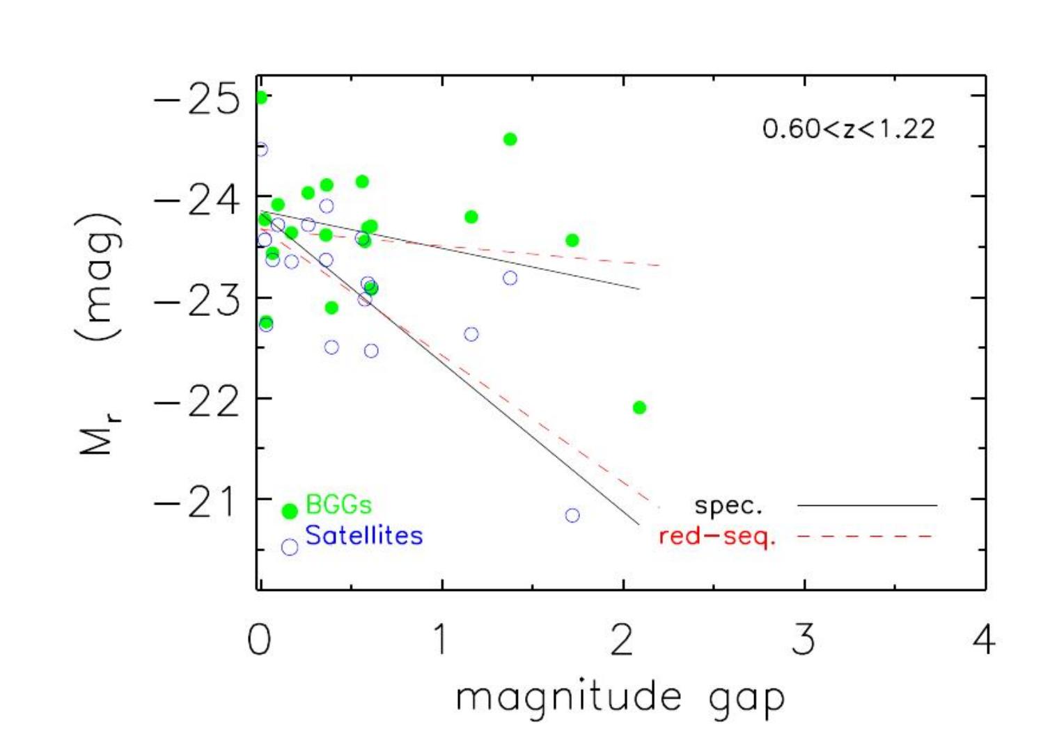
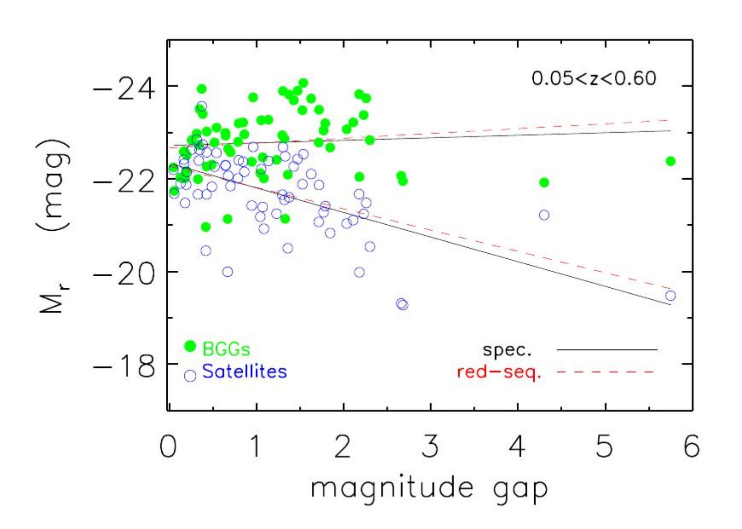
Figure 15: The absolute r-band magnitudes of the first (filled green circles) and the second (open blue circles) brightest galaxies as a function of the magnitude gap for the COSMOS+AEGIS+XMM-LSS sample of groups, having spectroscopic members. The solid black and dashed red lines show linear fits for the spectroscopic and red sequence selections of group membership, respectively. The upper panel and lower panel show the butterfly diagrams for high-z and low-z groups, respectively.

In §5.1 we examined whether contamination can affect the gap computations when the red-sequence method is applied for the selection of group membership versus the spectroscopic selection. In Fig. 15 we examine this effect on the butterfly diagrams, which are constructed using the spectroscopic sample of the COSMOS+AEGIS+XMM-LSS groups at z$<$0.6 (lower panel) and z$>$0.6 (upper panel). The redshift binning is limited by the sample size.

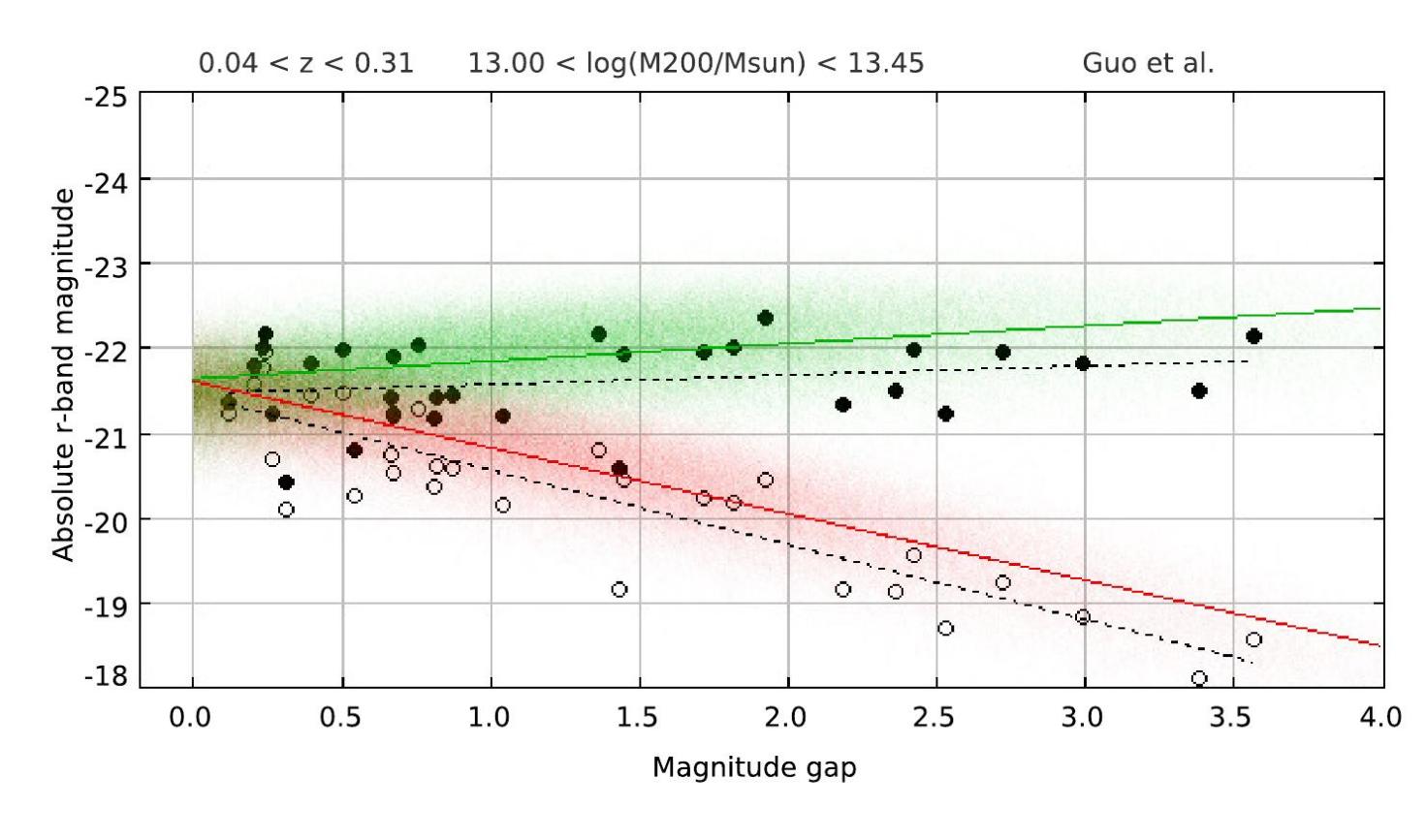
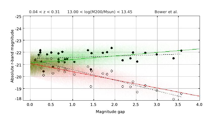
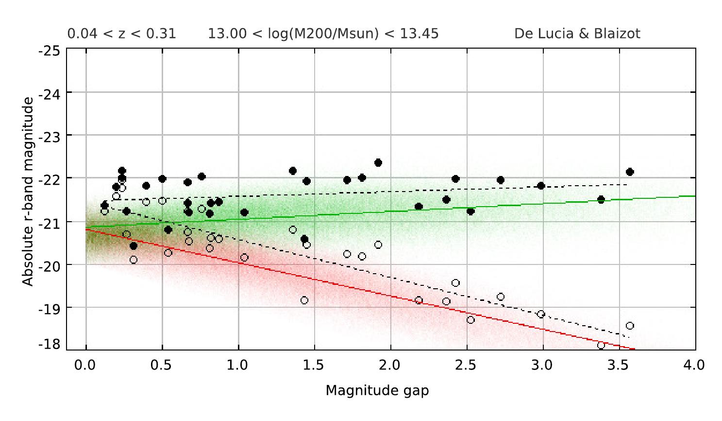
Figure 16: The absolute r-band magnitudes of the first and the second brightest galaxies as a function of the magnitude gap. The S–I data are shown by filled (BCG) and open (2-nd ranked galaxy) black circles with the dashed black lines showing the linear fit. Each panel shows the results of one of the SAMs (G11–top, B06–middle, DLB07–bottom), with green (red) points and a line showing the individual points and the fit to the BCG (2-nd ranked galaxy).

In Fig. 15 the filled green and open blue circles show the absolute r-band magnitudes of the spectroscopically selected BCGs and satellites as a function of $\Delta M_{1,2}$, respectively. These are quantified by linear regressions (solid black lines), $M_{r,1}=a_{1}+b_{1}\Delta M_{1,2}$ and $M_{r,2}=a_{2}+b_{2}\Delta M_{1,2}$. We have compared the results of these linear fits with those for the red-sequence selected BCGs and satellites (dashed red lines). Coefficients of fits are presented in Tab. 3. This comparison shows that the slopes of the red-sequence selection are slightly shallower than those for the spectroscopic membership and the membership contamination is a little more effective for the high-z groups compared to the low-z groups. However, the trends in the $M_{r,1}$ - $\Delta M_{1,2}$ and $M_{r,2}$ - $\Delta M_{1,2}$ relations for both red-sequence and spectroscopic members at z$<$0.6 and z$>$0.6 are similar and differences between the slopes/intercepts lie within the corresponding uncertainties. Thus, we expect that our findings which are derived from butterfly diagrams of our XMM-LSS catalog are valid within observational errors.

In Fig. 16, we compare the observed $M_{r,1}$–$\Delta M_{1,2}$ and $M_{r,2}$–$\Delta M_{1,2}$ relations with model predictions of G11 (top panel), B06 (middle panel) and DLB07 (bottom panel) for S–I. The observed luminosity of the first-ranked galaxy (filled black circles) increases very slowly with $\Delta M_{1,2}$, so the difference in the magnitude is due to the second-ranked galaxies (open black circles), which declines from $M_{r}\sim-21.5$ at $\Delta M_{1,2}\sim$0 to $M_{r}\sim$-18 at $\Delta M_{1,2}\sim$3.5. The values of the linear fit coefficients are given in Tab. 3. For S–I, the galaxies in the G11 model are more luminous than the observed galaxies by $\sim$0.3 mag. In contrast, galaxies in the B06 and DLB07 models tend to be less luminous than the observed galaxies by $\sim$0.5 to 0.7 mag.

For the S–II, a similar comparison is presented in Fig.17. The increase in the absolute magnitude of the BCG with $\Delta M_{1,2}$ is $\approx$3 higher than in S–I, reaching -22.5 at $\Delta M_{1,2}\sim$3.5. The absolute magnitude of the satellite galaxy declines from $M_{r}\sim$-21.5 at $\Delta M_{1,2}\sim$0 to $M_{r}\sim$-19 at $\Delta M_{1,2}\sim$3.5. As in S–I, the galaxies in the G11 model tend to be 0.5 mag more luminous than the observed ones. The B06 model predicts reasonably well the observed luminosity of the first-ranked and second ranked galaxies as a function of $\Delta M_{1,2}$. The predicted luminosities of galaxies in the DLB07 model are less luminous than the observed ones.

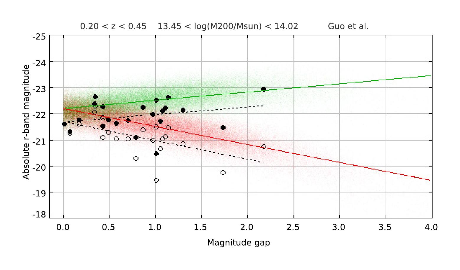
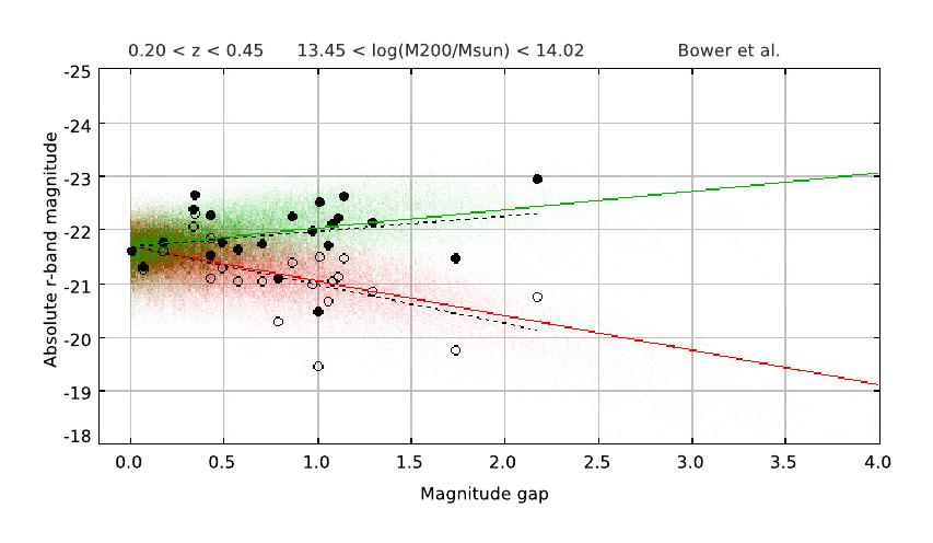
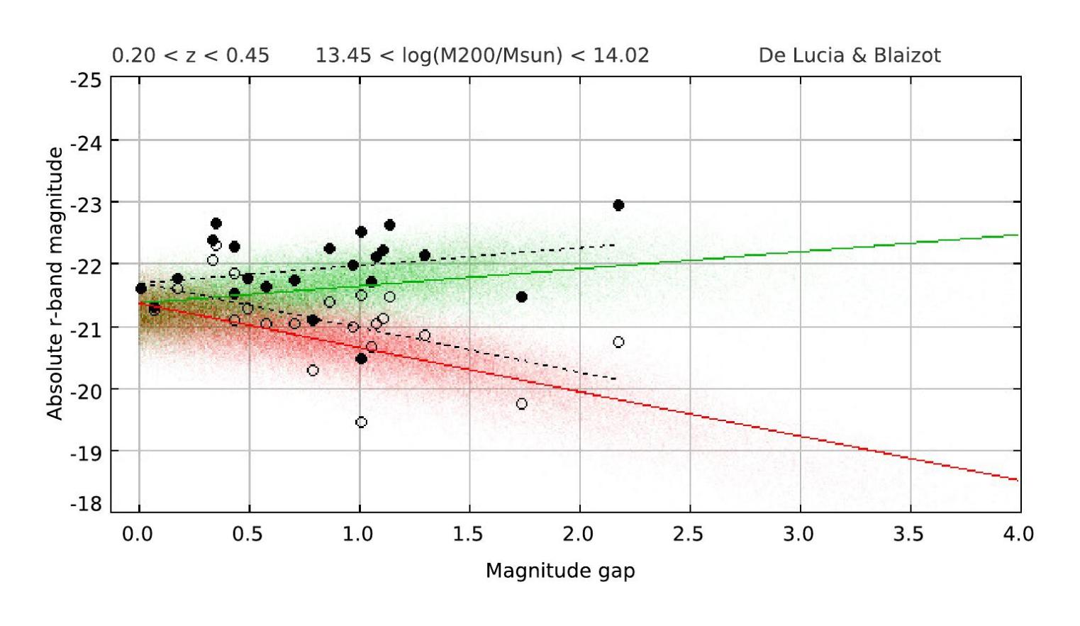
Figure 17: Same as in Fig. 16 , but for the BCGs and second brightest satellites in S–II.

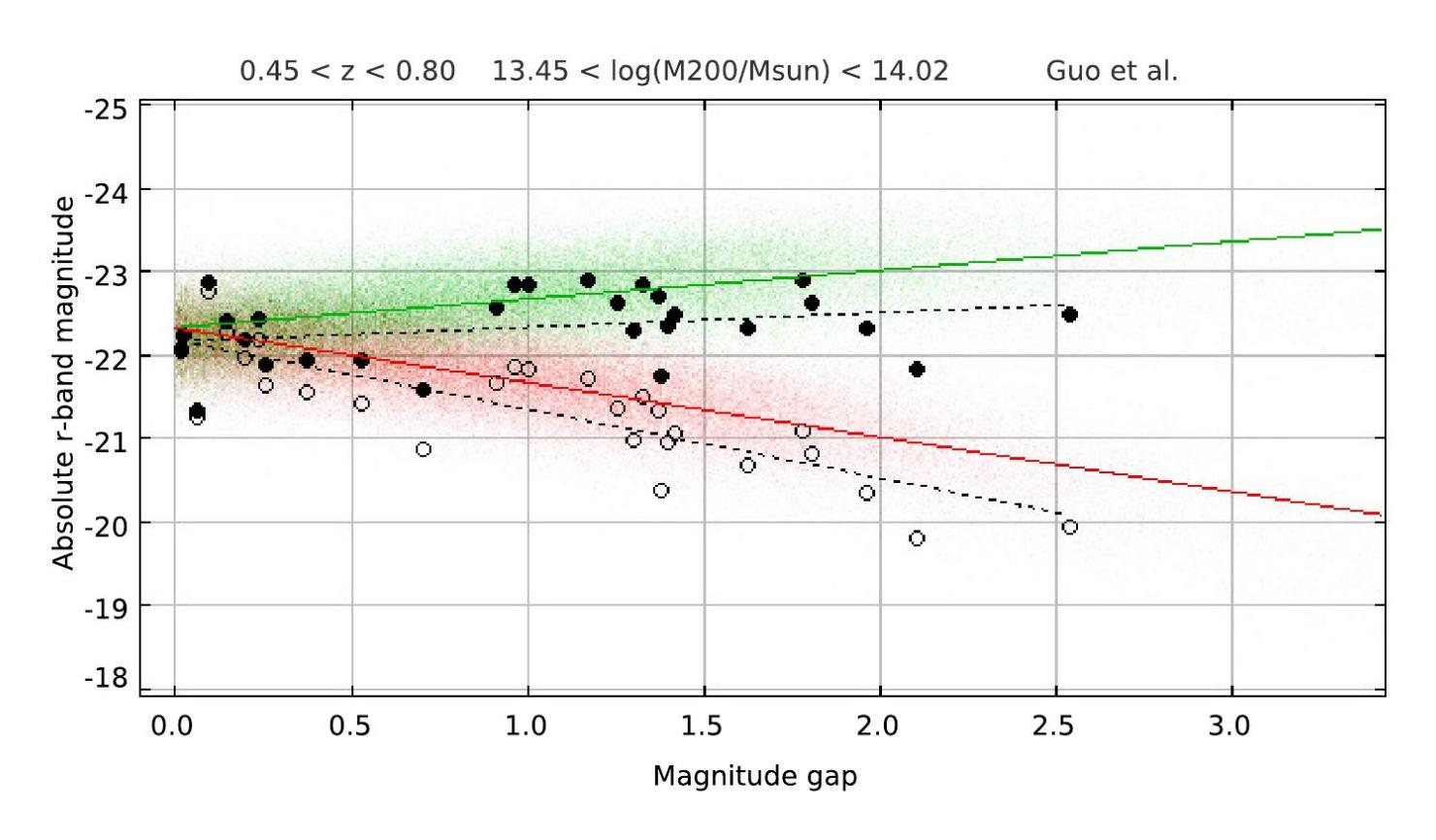
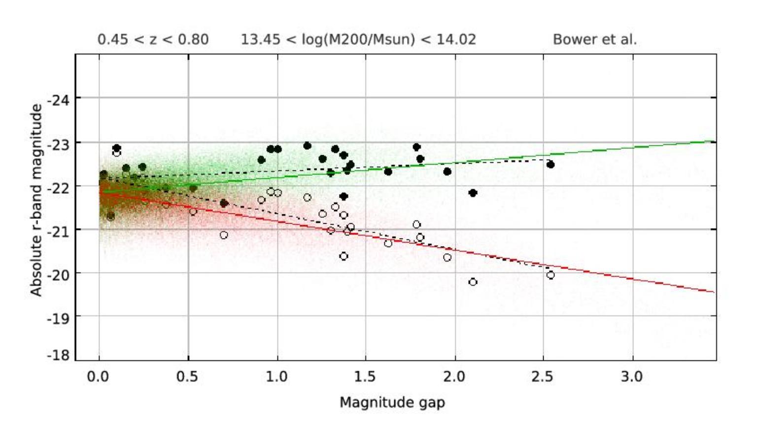
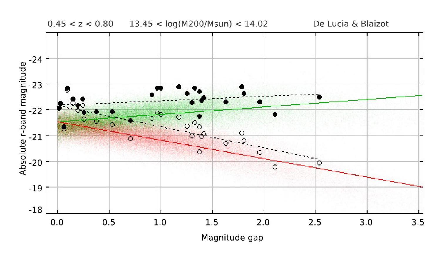
Figure 18: Same as in Fig. 16, but for the BCGs and second brightest satellites in S–III.

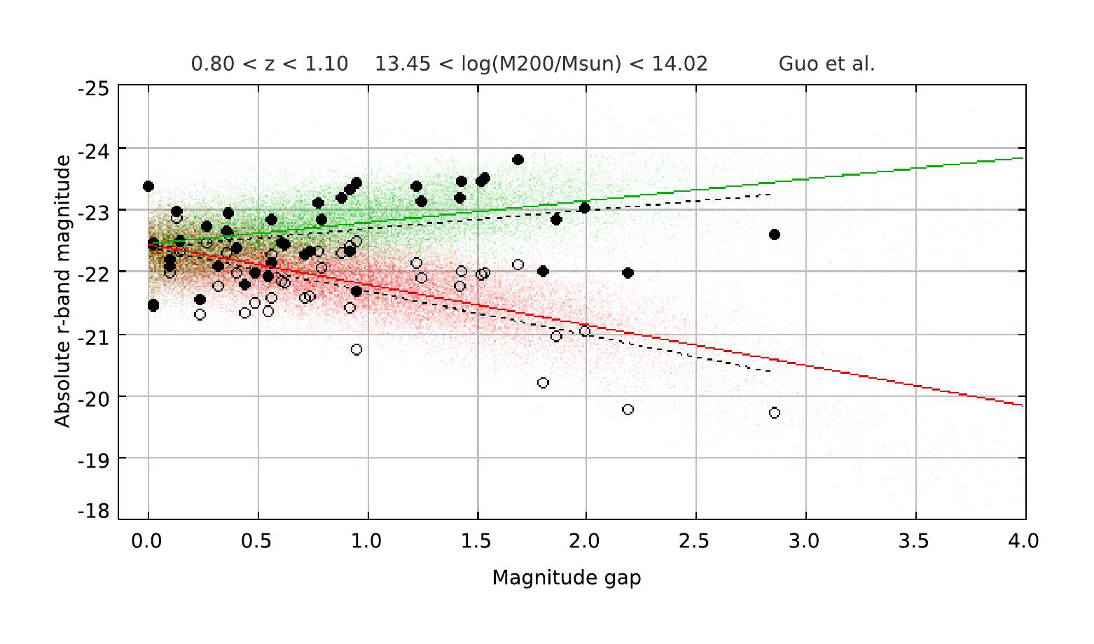
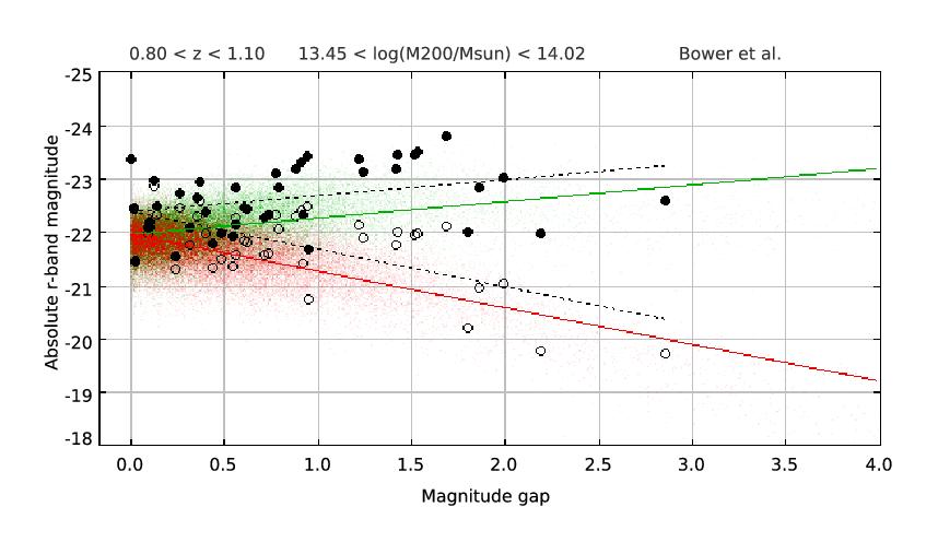
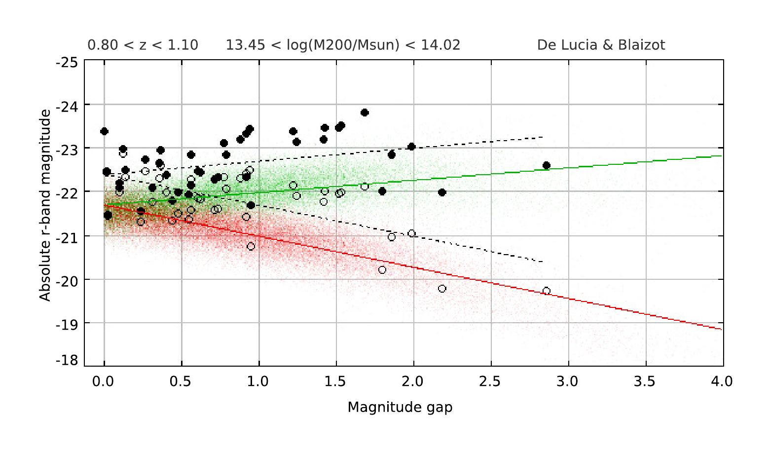
Figure 19: Same as in Fig. 16, but for the BCGs and the second brightest satellites in S–IV.

We show the butterfly diagrams for S–III in Fig. 18. As for the low-z subsamples, the luminosity of the BCG rises very slowly with $\Delta M_{1,2}$, spanning a range of -23$\lesssim M_{r}\lesssim$-21 with $\Delta M_{1,2}$. While, the luminosity of the satellite galaxy decreases from $M_{r}\sim$-22 at $\Delta M_{1,2}\sim$0 to $M_{r}\sim$-19 at $\Delta M_{1,2}\sim$ 3.5.

Finally, Fig. 19 illustrates the luminosities of BCG and 2-nd ranked galaxy as a function of magnitude gap for S–IV. The BCG absolute magnitudes span a range of -24$\lesssim M_{r}\lesssim$-21.5 and increase slowly with $\Delta M_{1,2}$. The luminosity of the second ranked galaxy declines from $M_{r}\sim$-22.5 at $\Delta M_{1,2}\sim$0 to $M_{r}\sim$-20 at $\Delta M_{1,2}\sim$3.5.

Table 3: The Best linear fit to the $M_{1,r}$ and $M_{2,r}$ as a function of $\Delta M_{1,2}$. The four upper rows present coefficients of the linear fit to the butterfly diagrams of our catalog and four lower rows list those for the sample of 84 groups from COSMOS+AEGIS+XMM-LSS.

Subsample	Mean redshift	a1	b1	a2	b2
XMM-LSS (our catalog)
S–I	0.175	$-21.44\pm 0.11$	$-0.11\pm 0.10$	$-21.42\pm 0.17$	$0.88\pm 0.11$
S–II	0.325	$-21.66\pm 0.22$	$-0.28\pm 0.15$	$-21.67\pm 0.22$	$0.72\pm 0.20$
S–III	0.625	$-22.13\pm 0.15$	$-0.19\pm 0.12$	$-22.14\pm 0.15$	$0.82\pm 0.13$
S–IV	0.95	$-22.35\pm 0.15$	$-0.30\pm 0.08$	$-22.35\pm 0.16$	$0.70\pm 0.16$
COSMOS+AEGIS+XMM-LSS
red-sequence selection	0.3	$-22.67\pm 0.15$	$-0.10\pm 0.10$	$-22.28\pm 0.14$	$0.46\pm 0.10$
spectroscopic selection	0.3	$-22.72\pm 0.14$	$-0.05\pm 0.09$	$-22.34\pm 0.14$	$0.53\pm 0.09$
red-sequence selection	0.9	$-23.67\pm 0.23$	$0.16\pm 0.34$	$-23.69\pm 0.23$	$1.26\pm 0.33$
spectroscopic selection	0.9	$-23.86\pm 0.21$	$0.37\pm 0.26$	$-23.83\pm 0.20$	$1.48\pm 0.25$

6.2.2 Redshift evolution of the butterfly diagram

In Fig.20, we compare the redshift evolution of the intercept of $M_{r,1}-\Delta M_{1,2}$ (top panel) and $M_{r,2}-\Delta M_{1,2}$ (bottom panel) relations in our observations and the models. We find a significant negative redshift evolution of the intercepts for BCGs and their satellites by $\sim$0.8 mag for clusters at z$\gtrsim$0.25. All models exhibit a shallower evolution of the intercepts with redshift compared to the data. A steeper negative evolution in the BCG magnitudes in time, is most likely due to younger stellar population age of BCGs, compared to the models. The intercept of the predicted butterfly diagram for S–I at low redshifts tend to be closer to G11 compared to two other models, indicating importance of their advances in the modeling. A possible reason for over-prediction of the BCG or BGG luminosity in G11 is that this model incorporates a disruption mechanism which provides additional gas and metal-rich material for the hot gas atmosphere of BCG, thus increasing the cooling rate and star formation in BCG (see G11). To achieve a good agreement with observations, it may still be needed to increase slightly the strength of AGN feedback in this model.

In Fig. 21, we show a lack of the redshift evolution in the slope of the butterfly diagram. No dependence on the absolute magnitude of BCG and an agreement between all models, indicates that the mechanism for creating large gaps is not strongly affected by the star-formation and feedback, and is due to disruption of galaxies. However, as we discussed above, the models show differences in the fraction of high gap systems, which is controlled by the efficiency of the transformation.

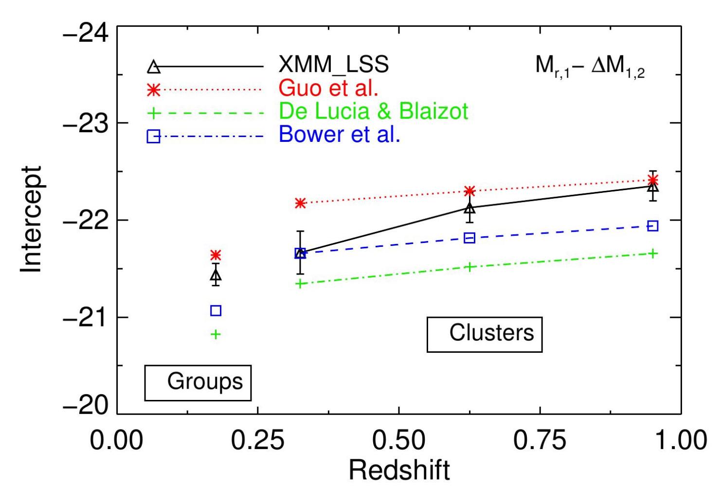
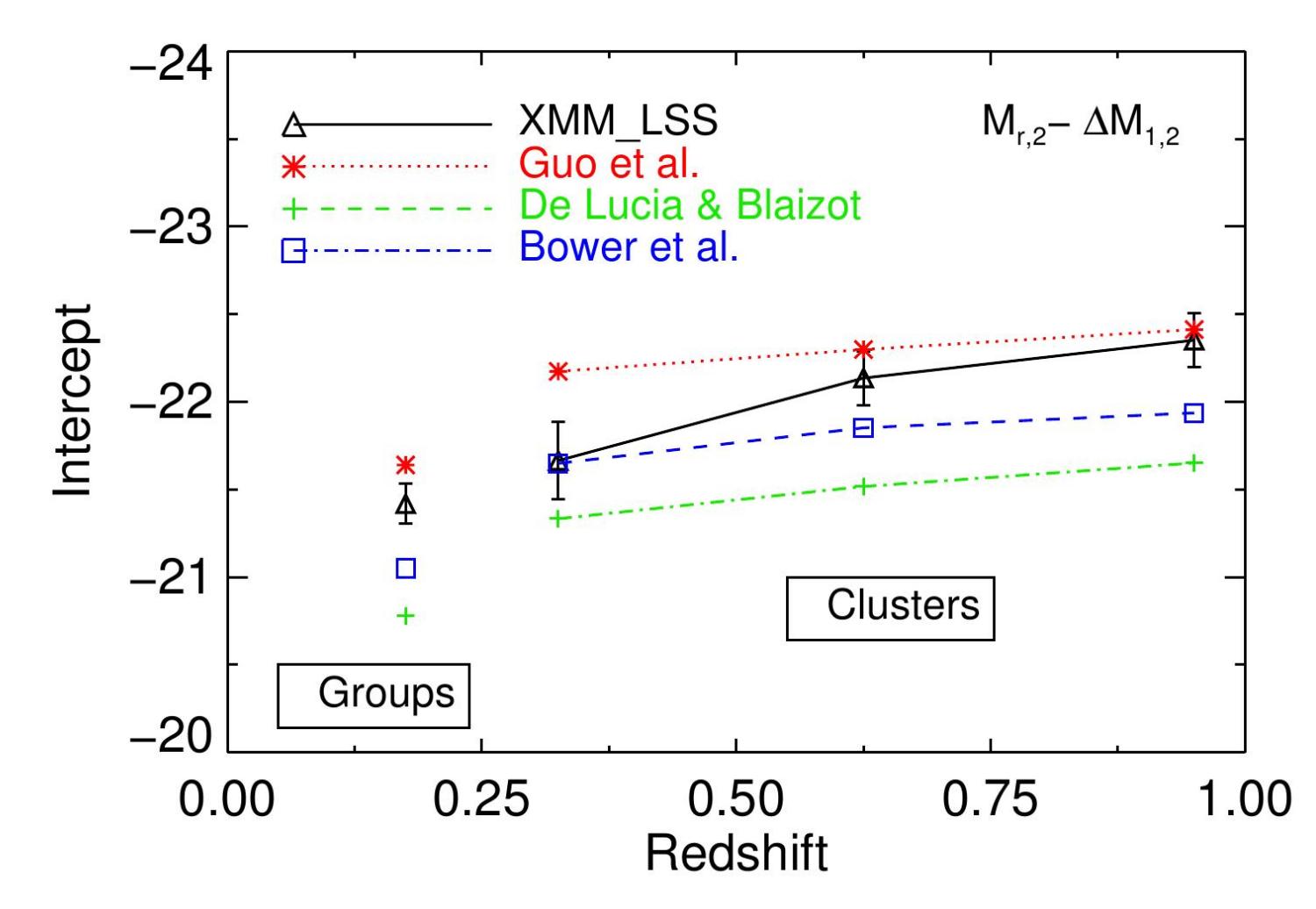
Figure 20: Evolution of the zero point of the $M_{r,1}$–$\Delta M_{1,2}$ (upper panel.) and $M_{r,2}$– $\Delta M_{1,2}$ (bottom panel.) relations with redshift. The solid black curve with error bars represents the data. Dotted red, dashed blue and dash-dotted green curves show the model predictions of G11, B06 and DLB07, respectively. In contrast to the models, we observe a significant evolution with redshift.

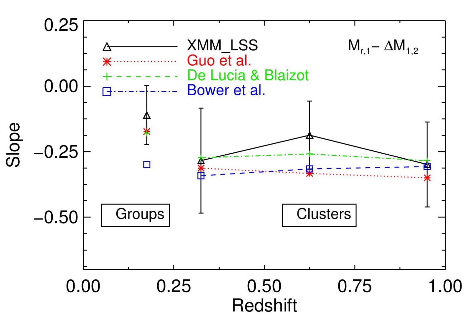
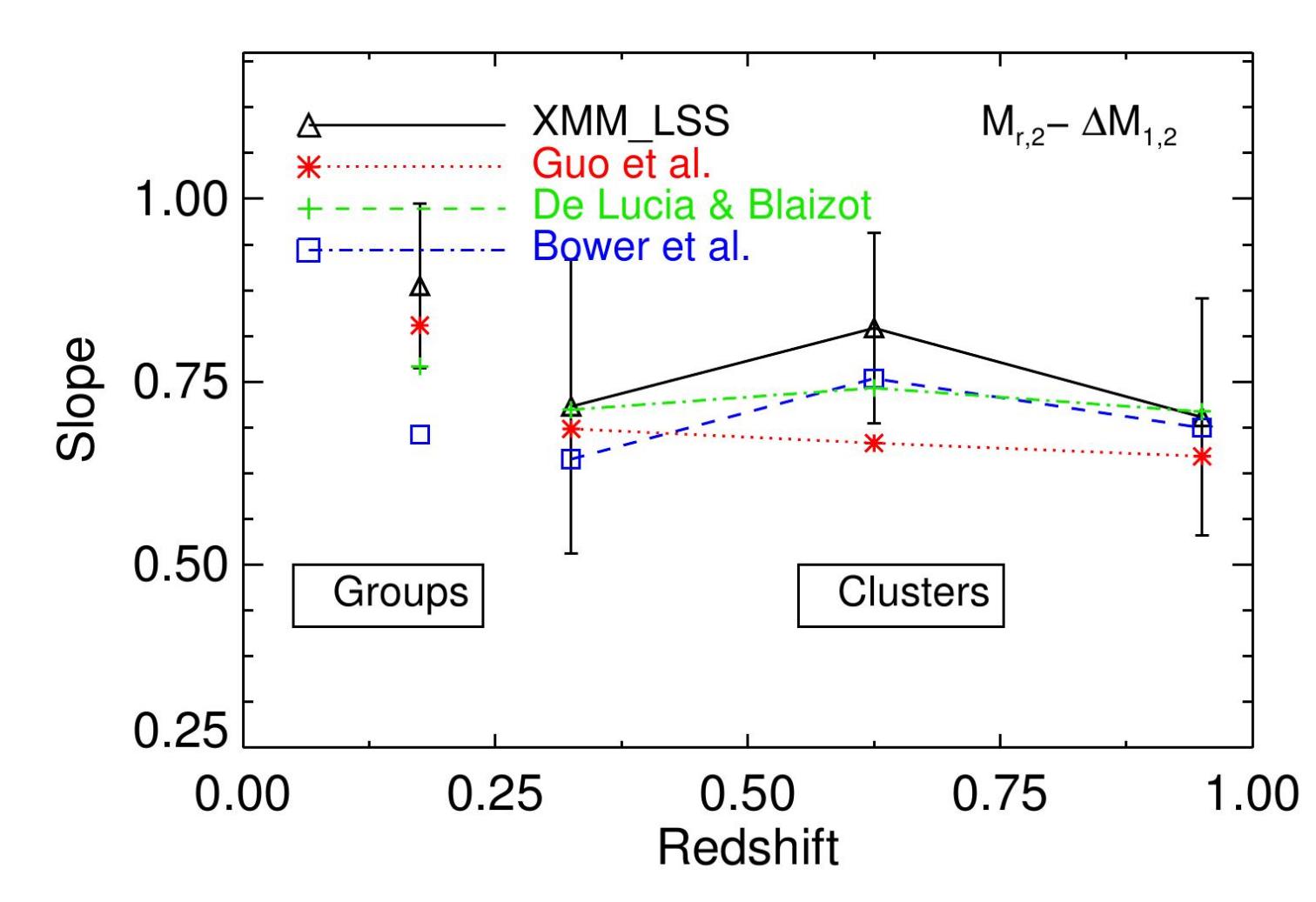
Figure 21: Evolution of the slopes of the $M_{r,1}$–$\Delta M_{1,2}$ (upper panel.) and $M_{r,2}$– $\Delta M_{1,2}$ (bottom panel.) relations with redshift. The models and the data reveal a nearly constant evolution with redshift.

6.3 Fossil groups

Using the magnitude gap, we identify 23 fossil groups in our catalog. The fossil groups constitute 22.2$\pm$6% and 12.3$\pm$7.0% of all identified X-ray groups in our catalog at z$\leq$ 0.6 and z$>$0.6, respectively. In this calculation we include the impact of the contamination (when using the red-sequence method versus the spectroscopic approach to select group membership) and completeness effects on the gap measurements. This misclassification causes the fraction of fossil groups to be underestimated by $\pm 20$% at high-z, which we add to the errors. Although the significance of the redshift evolution of the fraction of the fossil groups is marginal, it is also found in a nearly independent sample of the COSMOS+AEGIS+XMM-LSS groups, which contains 23.1$\pm$7% and 10.5$\pm$8% of all groups as fossil groups at z$\leq$ 0.6 and z$>$0.6, respectively.

We mark the fossil groups in Fig. 7 with red circles to illustrate their occurrence as a function of total mass and redshift. Given the previous results on the prevalence of cool cores among the fossil groups, in the following we verify that we do not have a preferential selection of the fossil groups. Given the limited statistics of the X-ray data, we select the extent of X-ray detection as a parameter of the comparison. If the extends are much smaller, it would indicate that the central part of the emission dominates the detection and the X-ray selection of fossils is different to the bulk of the groups.

We compare the distributions of $\frac{R_{X}}{R_{500}}$ ratio for fossils to non-fossils, selected by implying $\Delta M_{1,2}\leq$0.5 in Fig. 22 (top panel). $R_{X}$ is the detected extent of the X-ray emission, while $R_{500}$ is the extent of X-ray emission anticipated for the given flux of the group. The distribution of $\frac{R_{X}}{R_{500}}$ ratio is skewed toward the lower values for fossils compared to the non-fossil groups, with 1% probability of chance occurrence, based on the K-S test. However, as also shown in Fig. 22, the observed extent of the X-ray emission is a strong function of the redshift of the group. So, for a refined comparison of the extent of X-ray detection for fossil candidates and non-fossils, we separate the groups into two redshift bins: with z$>$0.6 and z$\leq$0.6. We find that fossils exhibit only a marginally lower values of $\frac{R_{X}}{R_{500}}$ ratio compared to non-fossils in both redshift ranges, z$>$0.6 and z$\leq$0.6, which may also be due to residual differences in the redshift distribution. In our method, the cores of groups are removed prior to detection, which as this test shows, reduces the impact of X-ray selection.

In Fig. 23 to Fig. 44 we show the X-ray emission as contours on the CFHTLS RGB images for the fossils candidate groups listed in Tab. 4. We show the color magnitude diagrams of g^′-r^′ and r ^′- i^′ versus z^′ for the fossil candidates at z$<$0.66, and r ^′-i ^′ and i ^′-z^′ versus z^′ for those at z$\geq$0.66. Group members (dark circles) are selected according to the method described in §4.1. We mark the BGG and the second brightest galaxies on each RGB image and all color magnitude diagrams.

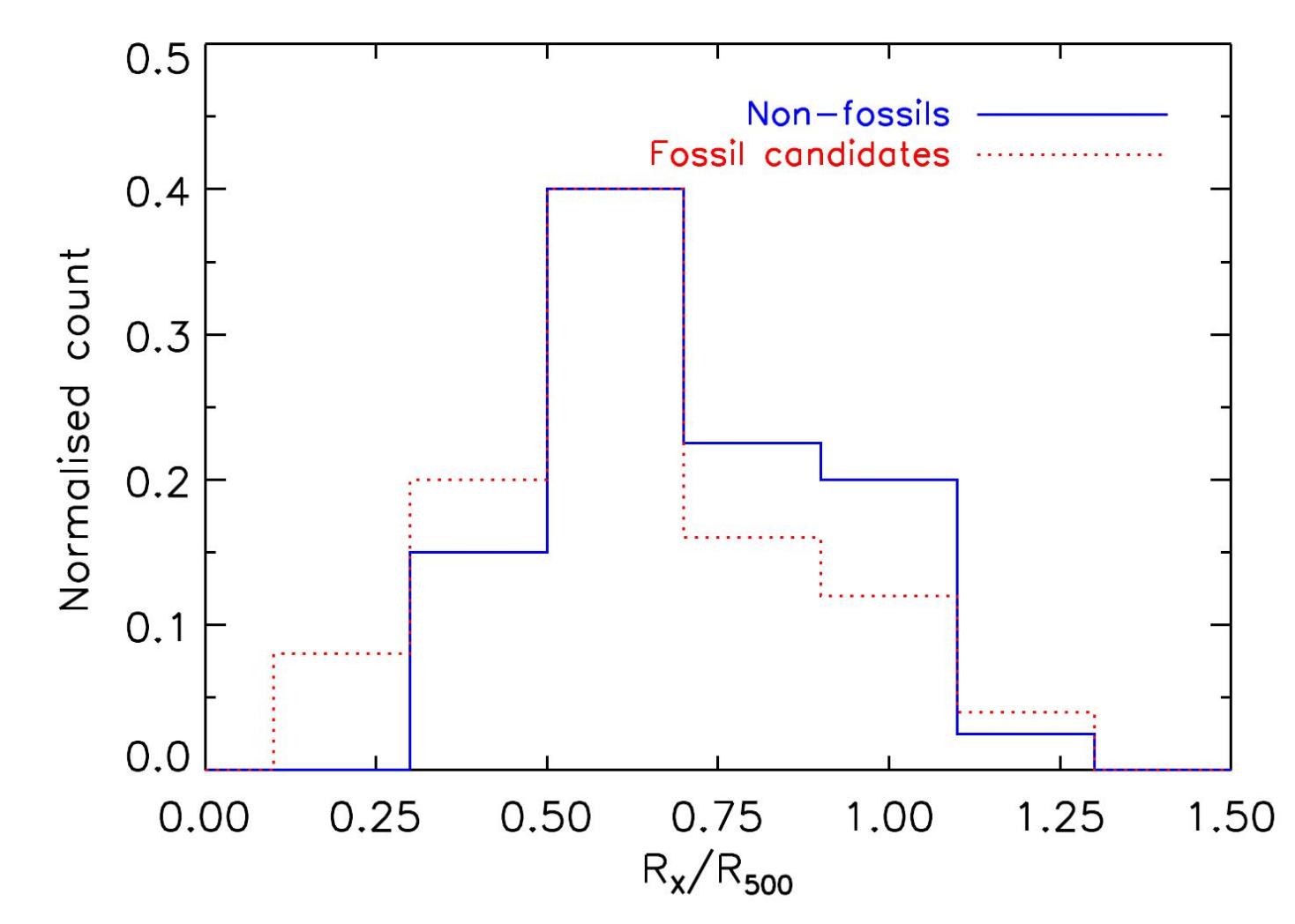
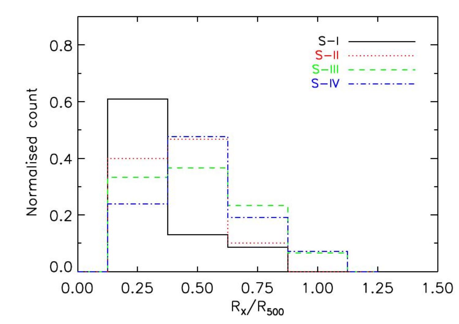
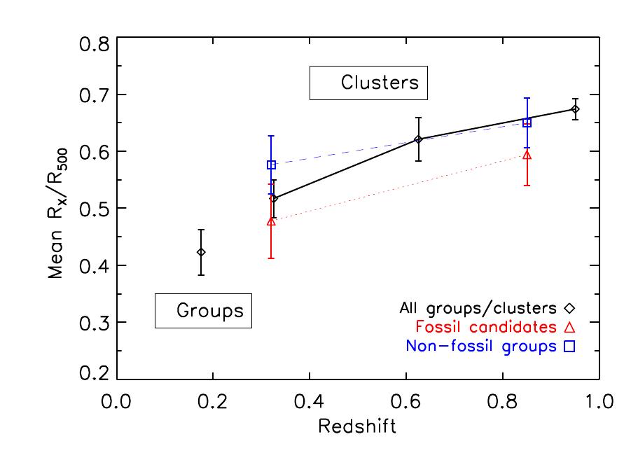
Figure 22: Upper panel. Distribution of the ratio of the X-ray extent of the detection to the total extent of X-ray emission, $\frac{R_{X}}{R_{500}}$ for the fossil group candidates ($\Delta M_{1,2}\geq$1.7) (dotted blue histogram) and non-fossils ($\Delta M_{1,2}\leq$0.5) (solid red histogram) in our X-ray group catalog. The fraction of fossil groups is skewed toward the lower values of $\frac{R_{X}}{R_{500}}$ compared to the non-fossil groups. Middle panel. The $\frac{R_{X}}{R_{500}}$ distribution for X-ray groups in different subsamples. Lower panel. The redshift evolution of the extent of X-ray detection for galaxy groups/clusters. A redshift evolution in the ratio by 0.25 in amplitude is seen for all groups.

7 Summary and conclusions

We search for the extended X-ray emission using the contiguous XMM coverage of the CFHTLS W1 field by the XMM–LSS public data. We provide a catalog of 129 X-ray galaxy groups including 44 groups with a spectroscopic redshift over $\sim$3 degrees², spanning the redshift range 0.04$<$z$<$1.23, characterised by a rest frame 0.1–2.4 keV band luminosity range between $10^{41}$ and $10^{44}$ ergs s^-1. We utilize a two-color red-sequence finder for the photometric selection of group members and to calculate the mean group redshift. For the first time, we perform a statistical analysis on the luminosity gap of groups over the wide redshift range of our catalog. We compare our observational results with predictions of SAMs presented in G11, DLB07 and B06. Our main results are as follows:

(i) We have compared the flux for the groups and clusters in common with the C1 clusters of Adami et al. (2011). We show that clusters at z$>0.6$ have important differences in flux estimates as a consequence of point source contamination.

(ii) We show that two color selection of group members reduces the sample contamination by DSFGs at $\lesssim$0.6 compared to a single color selection. This contamination slightly affects the sample at z$\gtrsim$0.6 (by $\approx$3%).

In addition, to test the effect of a red sequence selection of members on the magnitude gap measurements and the determination of the fraction of fossil or non-fossil groups, we compare the magnitude gap values computed using the spectroscopic and red sequence members for a sample of 84 spectroscopic X-ray groups from our catalogs in the AEGIS, COSMOS and XMM-LSS fields. We find that the systematic effect on the magnitude gap computation is limited to $<6$ % at 95% Poisson confidence level, which is low compared to our statistical uncertainties. We apply this effect on our estimate of the fraction of fossil groups and number of groups in each $\Delta M_{1,2}$ bin in Fig. 12. Using this sample we show that our results which are derived by combining groups with red-sequence and spectroscopic membership are valid and we quantified the corresponding uncertainties.

(iii) We demonstrate that the fraction of groups as a function of $\Delta M_{1,2}$ exhibits a flatter slope for low-z and low-mass groups in S–I compared to higher redshift subsamples, revealing the build-up of high magnitude gap groups at low redshift. We derive a marginally higher fraction of groups with $\Delta M_{1,2}\geq$2 compared to all models for S–I. We find that the B06 model is not able to reproduce the observed trends for $\Delta M_{1,2}$ distributions. On the other hand, G11 and DLB07 models predict reasonably well $\Delta M_{1,2}$ distributions for groups and clusters.

It appears that the magnitude gap distribution of groups with $\Delta M_{1,2}\lesssim$2 is well modeled by these two models. However the consistency between them and observations is reduced for groups and clusters with large magnitude gap, such as fossil groups, indicating that the fraction of these objects have not been understood completely. We report a good agreement between distributions of the magnitude gap for our groups catalog with red sequence selection of group members and that of our spectroscopic sample of 84 groups within the redshift range of 0.05$<$z$<$1.22 (see Fig. 11).

(iv) We show that the model abundance by volume of galaxy groups is in agreement with low-z X-ray groups in S–I. However, at higher redshifts the observed number density of groups with higher halo masses is below the predicted model values which we attribute to cosmic variance and sensitivity of the abundance of high-mass systems to cosmological parameters. We demonstrate that the observed mean fraction of X-ray clusters with $\Delta M_{1,2}\geq$1 evolves slowly with redshift in agreement with all models, with the exception of B06, which under-predicts the fraction of clusters with $\Delta M_{1,2}\leq$1. A larger fraction of groups with $\Delta M_{1,2}\leq$1 is detected at lower redshifts, in agreement with the models.

(v) We investigate the absolute r-band magnitude of the first and the second brightest galaxies as a function of the magnitude gap. We find a significant negative evolution of the intercept ($\sim$0.8 mag) of the $M_{r,1}$ - $\Delta M_{1,2}$ and $M_{r,2}$ - $\Delta M_{1,2}$ relations for clusters at 0.2$\lesssim$z$\lesssim$1.10. In comparison, all the models predict a flatter redshift evolution for the intercepts. We attribute the steeper negative evolution in the BCG magnitudes to a more recent build-up of stellar mass in these galaxies (in agreement with the models), suggestive of a stronger redshift dependence of AGN feedback. The G11 model predicts well the intercepts for low-z and low-mass groups, indicating the importance of the improvements which have been made to this model. Conversely, B06 and DLB07 models under-predict the intercepts for the BGGs and their satellites. The observed slope of the $M_{r,1}-\Delta M_{1,2}$ and $M_{r,2}-\Delta M_{1,2}$ relations for clusters show a nearly constant redshift evolution, consistent with all models. We conclude that the mechanisms for creating magnitude gaps is well modeled in the SAMs. For galaxy groups, we find that the G11 and DLB07 models predict reasonably well the slopes of the butterfly diagrams. We conclude that satellite distribution in galaxy groups is too efficient in the B06 model.

(vi) We have selected 22 fossil group candidates using the magnitude gap criterion. Similar to other studies we find that fossil groups constitute 22.2$\pm$6% of all groups at z$<$0.6. We report a redshift evolution in this fraction which drops to 12.3$\pm$7% at z$>$0.6. These numbers and their evolution are consistent with those of our spectroscopic sample of COSMOS+AEGIS+XMM-LSS groups where we classify 23.1$\pm$7% and 10.5$\pm$8 % of all groups as fossils at z$\leq$0.6 and z$>$0.6, respectively. We show that some fossil group candidates include few galaxies, located outside the 0.5R₂₀₀, which are brighter than the second bright galaxy which used for the magnitude gap estimate, supporting a suggestion of Von Benda-Beckmann et al. (2008) that large magnitude gaps can be refilled by infall.

Finally, this study demonstrates that magnitude gap can be used to differentiate between models. We find that the recent improvements in the SAM of G11 brings it closer to the observations compared to the early version of the SAMs, DBL07 and B06. However, it still fails to reproduce all the results. For current SAMs only a single model output is available. However, in order to improve the understanding further, a grid of model predictions fully sampling the parameter space of amplitude and redshift evolution of the relevant physical mechanisms such as AGN feedback is essential.

8 Acknowledgements

Initial stages of this work have been partially funded by the German Deutsche Forschungsgemeinschaft, DFG Leibniz Prize $(FKZHA1850/28-1)$. This work also has been partially supported by the grant of Finish Academy of Sciences to the University of Helsinki, decision number 266918. We thank Guenther Hasinger, Hannu Koskinen, Kirpal Nandra, Christophe Adami, Birgit Boller, Marguerite Pierre, Peter Johansson and Kimmo Kettula for helpful assistance and comments. We thank the anonymous referee for the patience in reviewing the manuscript and many insightful comments. We used the Millennium Simulation databases in this paper and the web application providing online access to them were constructed as part of the activities of the German Astrophysical Virtual Observatory.

Appendix A Fossil group candidates

In Tab. A1 we present fossil group candidates catalog. Column 1 and column 2 are group id and the photometric redshift of group. Columns 3 and 4 present the BGG coordinate RA.(J2000) and Dec.(J2000) in degrees. Columns 5 and 6 are BGG r^′-band magnitude and $\Delta M_{1,2}$. In Figs. 23-44 we show the X-ray emission as contours overlaid on the CFHTLS RGB image (top panel) and the color magnitude diagrams of g^′ - r^′ and r^′ - i^′ versus z^′ for z $<0.6$ and r^′ - i^′ and i^′- z^′ versus z^′ for z $>0.6$ for fossil group candidates listed in Tab. 4.

In §5.2 we define a fossil group and the search radius used for the magnitude gap calculation. Group members selected using two colors according to the method described in §4.1. We show group members with filled black circles in each color magnitude diagrams. The first and second brightest galaxies are marked by red asterisks. The upper and lower limits of colors in each redshift have been shown with horizontal dotted blue lines.

As it can be seen in the color magnitude diagrams, in some galaxy groups there are galaxies outside the 0.5$R_{200}$ that are brighter than the second galaxy which is used to compute the $\Delta M_{1,2}$. These groups are experiencing the infall of galaxies into search radius. This demonstrates that the magnitude gap estimate and the identification of fossil groups are very sensitive to the adopted search radius for selecting the second bright galaxy.

Table 4: Fossil group candidates.

Group ID	zphot	RA${}_{BGG}(J2000)$	Dec${}_{BGG}(J2000)$	$r^{\prime}$	$\Delta M_{1,2}$
(1)	(2)	(3)	(4)	(5)	(6)
101540	0.07	36.3736	-4.0120	14.219	1.922
101391	0.07	36.1958	-4.1475	16.929	3.297
102820	0.11	36.9687	-3.8552	17.213	2.059
100130	0.13	36.8133	-5.0756	16.367	2.645
103330	0.14	35.3946	-4.038	17.142	6.922
101210	0.15	36.3319	-4.317	16.634	1.747
100150	0.16	35.2821	-4.9992	17.302	2.957
100010	0.22	36.4159	-5.0052	17.241	1.714
102130	0.23	35.6247	-3.8769	18.470	2.232
101290	0.25	36.6974	-4.2531	18.733	2.514
101480	0.34	36.6486	-4.0695	18.025	2.157
100640	0.34	35.5052	-4.6332	18.128	2.022
101200	0.47	35.6688	-4.3064	20.393	4.607
103320	0.53	36.5861	-3.7339	20.354	1.791
101730	0.6	36.0241	-3.9213	20.130	1.955
101360	0.6	36.8554	-4.1823	20.489	2.728
100620	0.66	37.1107	-4.6587	22.320	2.103
101000	0.76	35.8876	-4.4227	21.136	1.727
102220	0.86	35.7790	-3.7906	22.957	2.187
100120	0.88	35.3644	-5.067	22.125	3.080
101490	0.94	35.3728	-4.0977	22.336	1.989
100430	0.98	36.1239	-4.8010	22.342	1.861
101120	1.1	35.5422	-4.3494	21.181	2.808

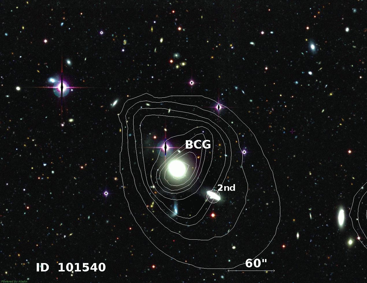
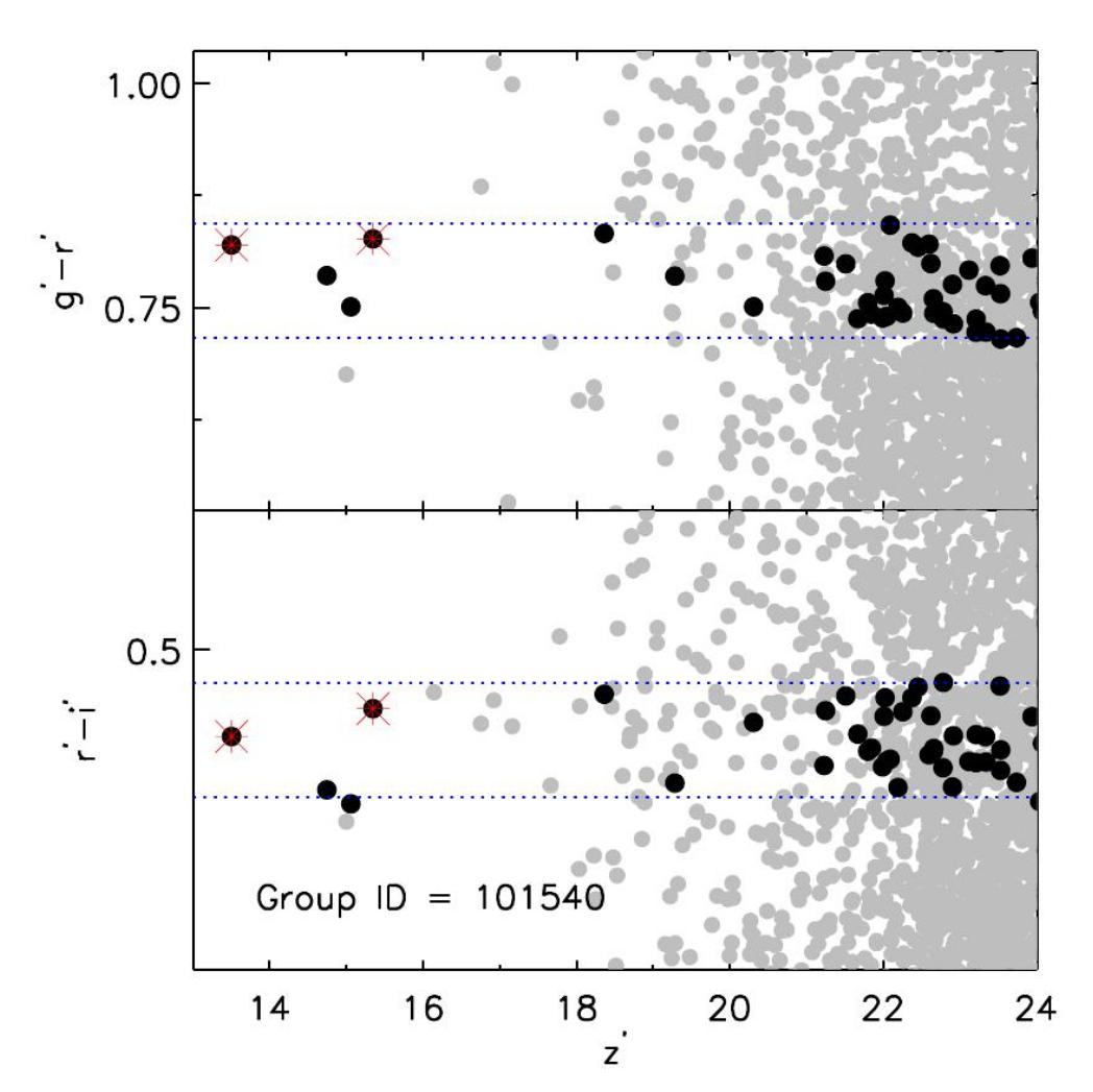
Figure 23: Upper panel. Contours of the extended X-ray emission overlaid on the CFHTLS RGB image of the fossil group 101540 at z=0.07. Middle panel. g^′- r^′ versus z^′. Lower panel. r^′ - i^′ versus z^′. Filled black circles illustrate group members selected by the method described in §4.1. The BGG and second brightest satellite galaxy within $0.5R_{200}$ have been marked with red asterisks within each color magnitude diagram. The upper and lower limits of colors have been shown by horizontal dashed lines.

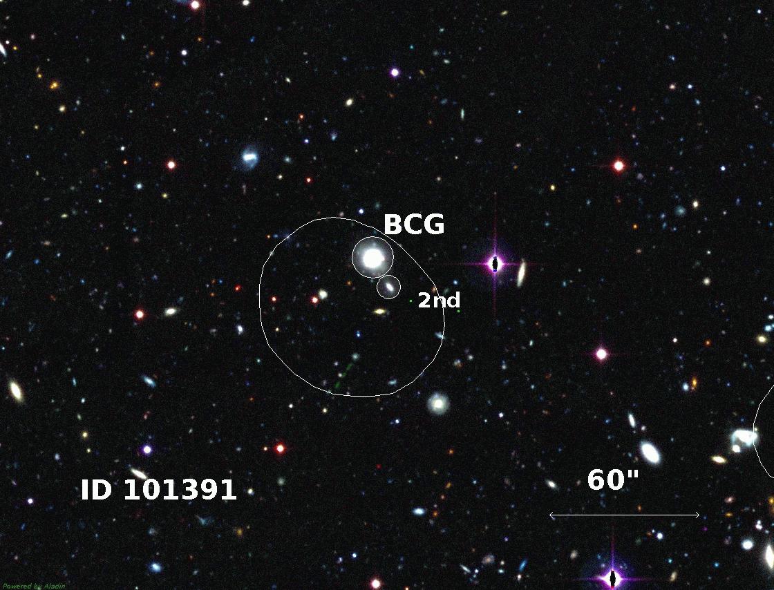
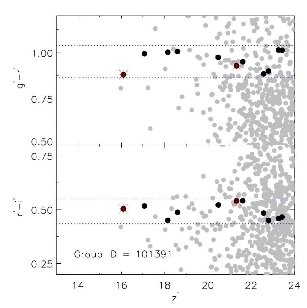
Figure 24: Same as in Fig. 23, but for the group 101391 at z= 0.07.

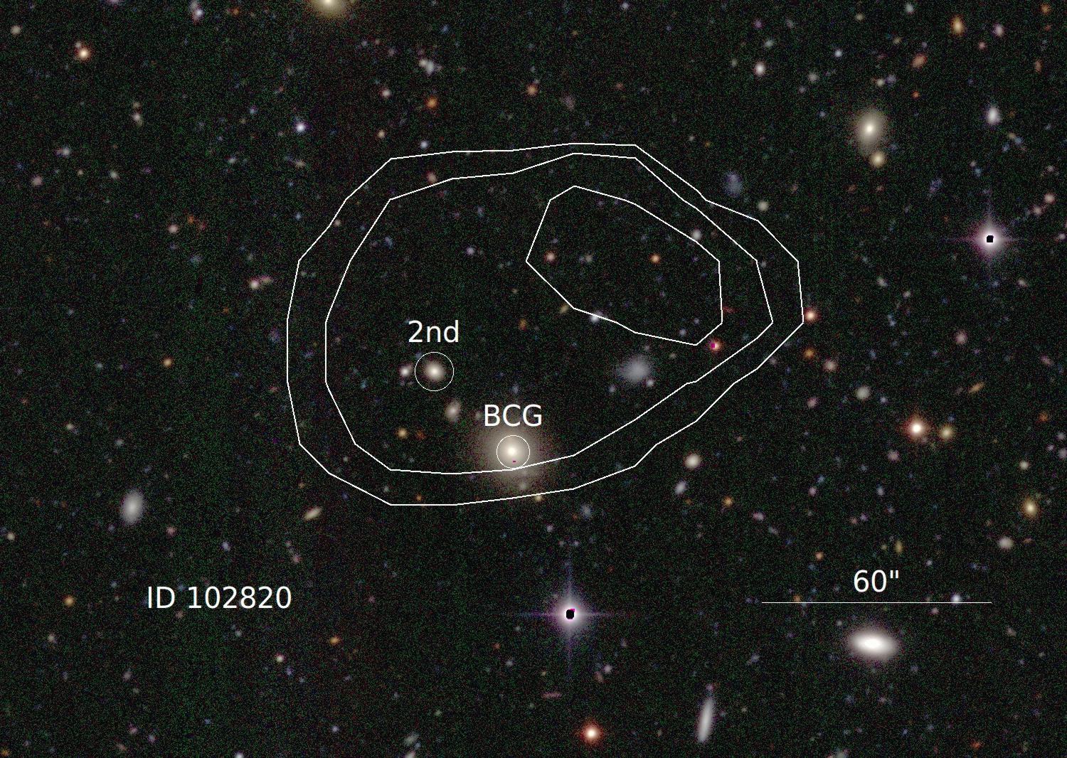
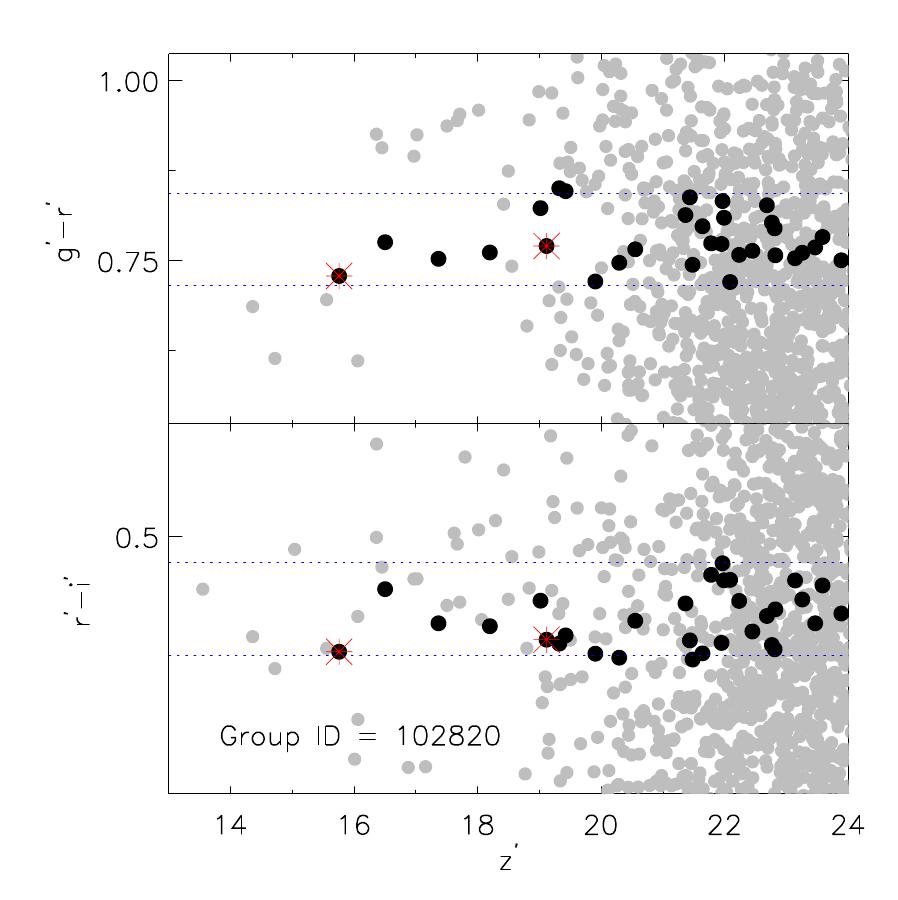
Figure 25: Same as in Fig. 23, but for the group 102820 at z=0.11.

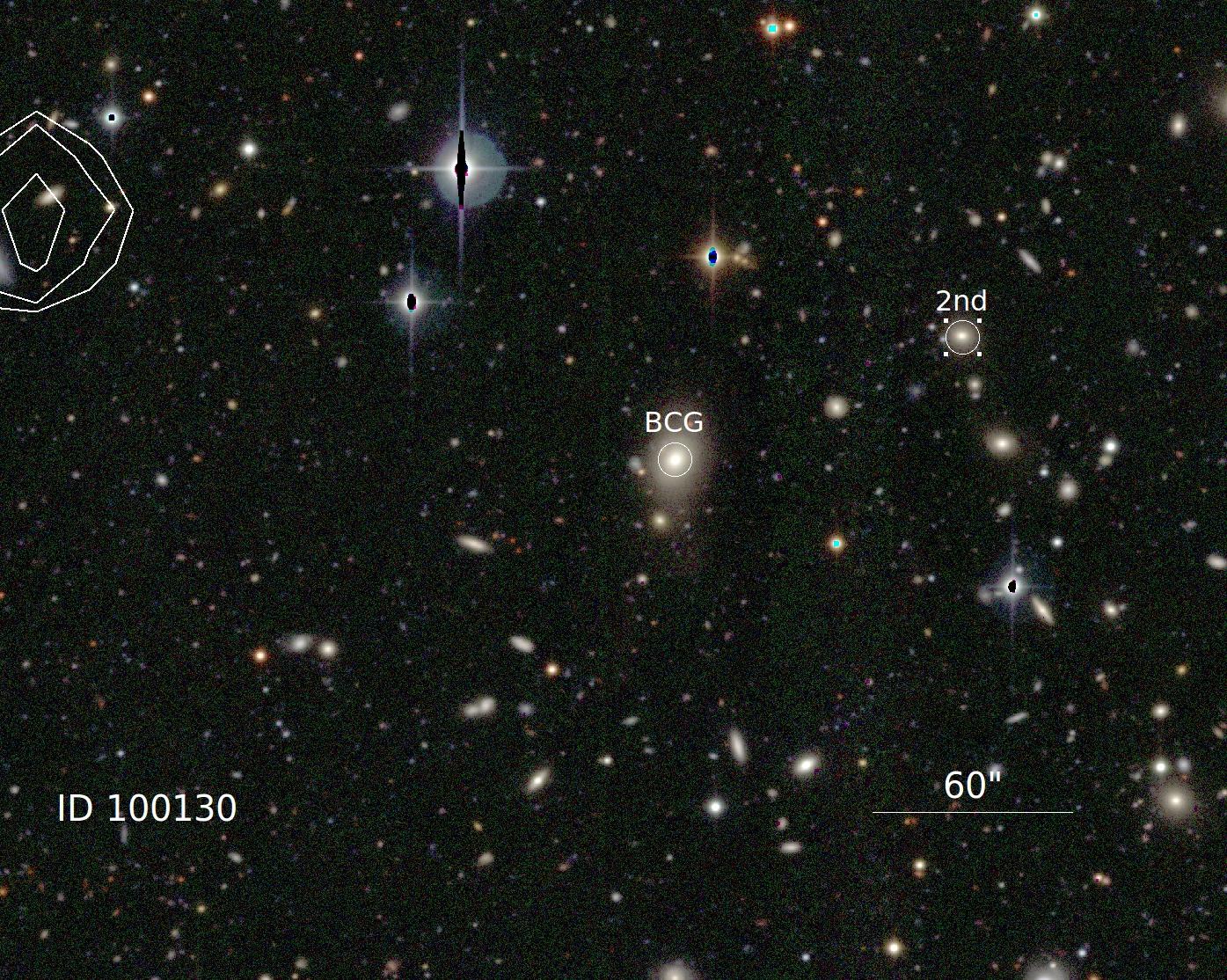
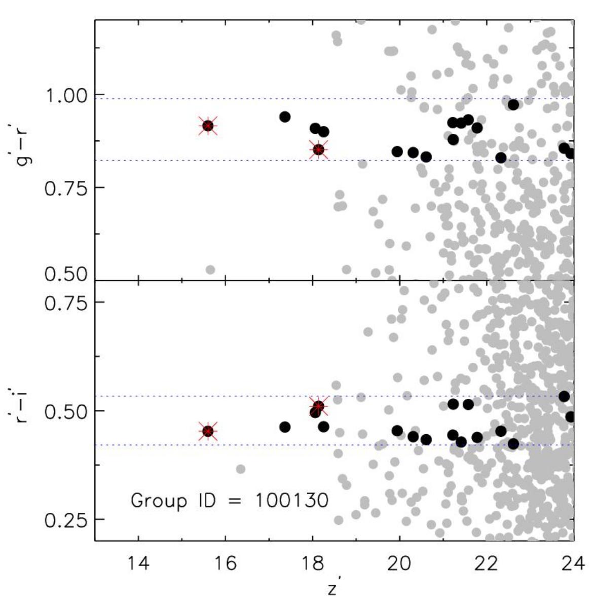
Figure 26: Same as in Fig. 23, but for the group 100130, at z= 0.13.

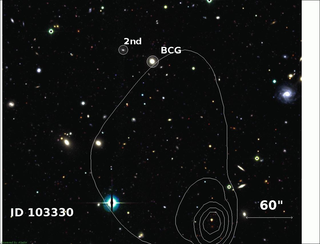
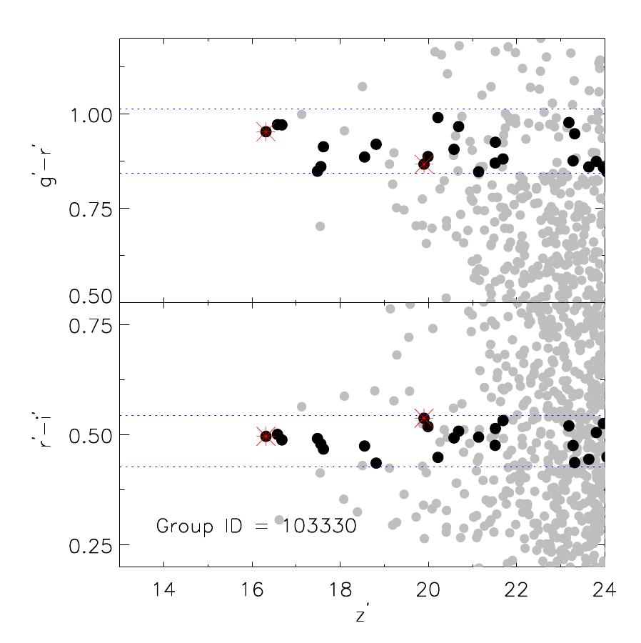
Figure 27: Same as in Fig. 23, but for the group 103330 at z= 0.14.

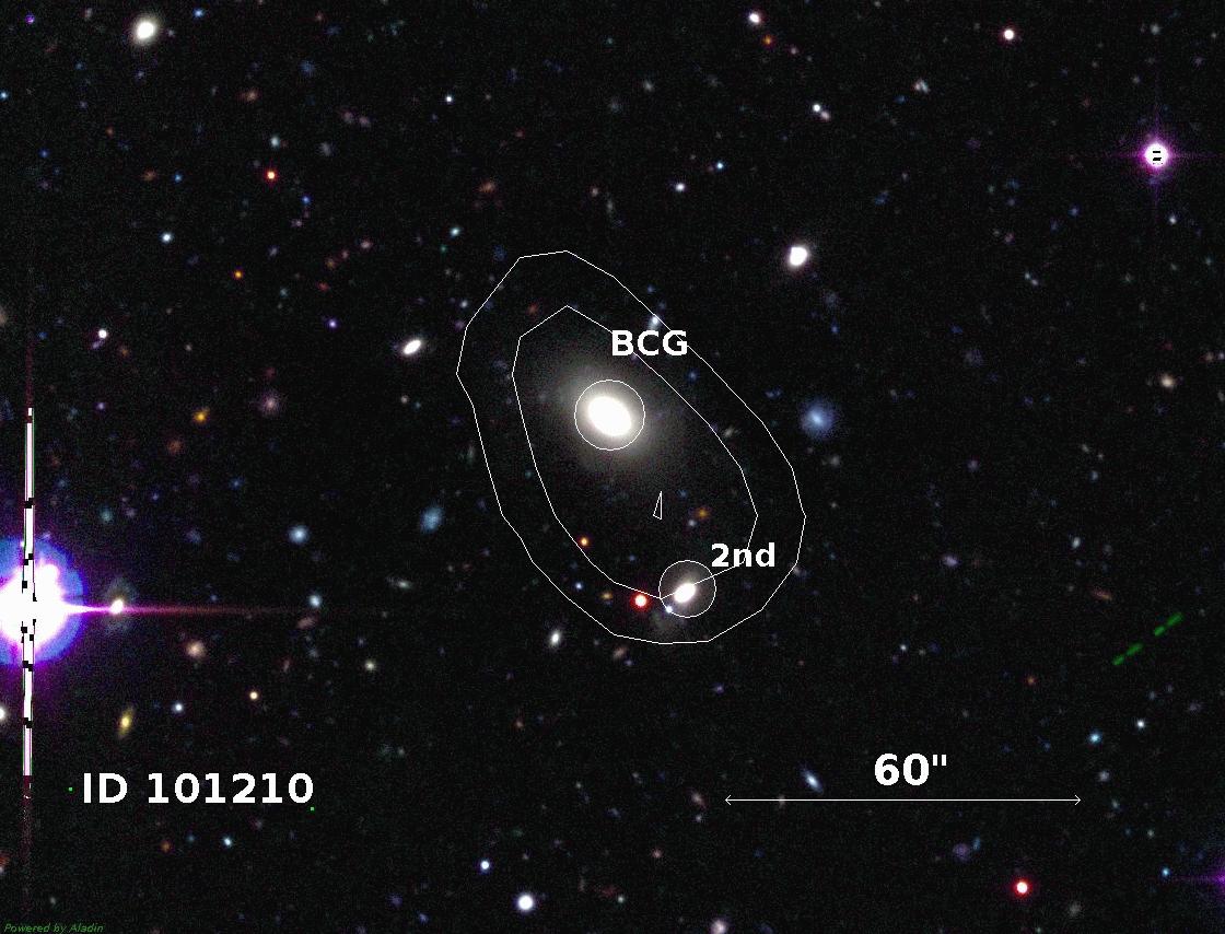
Figure 28: Same as in Fig. 23, but for the group 101210 at z= 0.15.

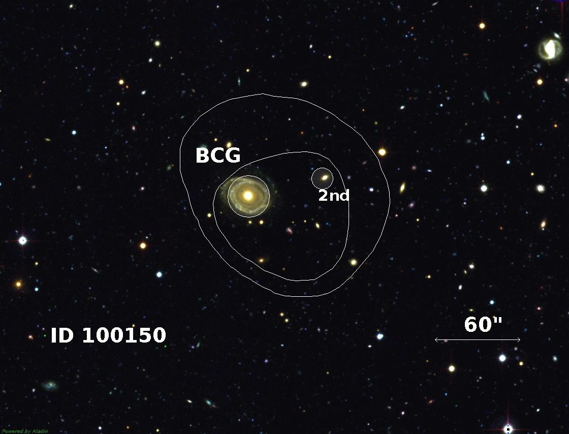
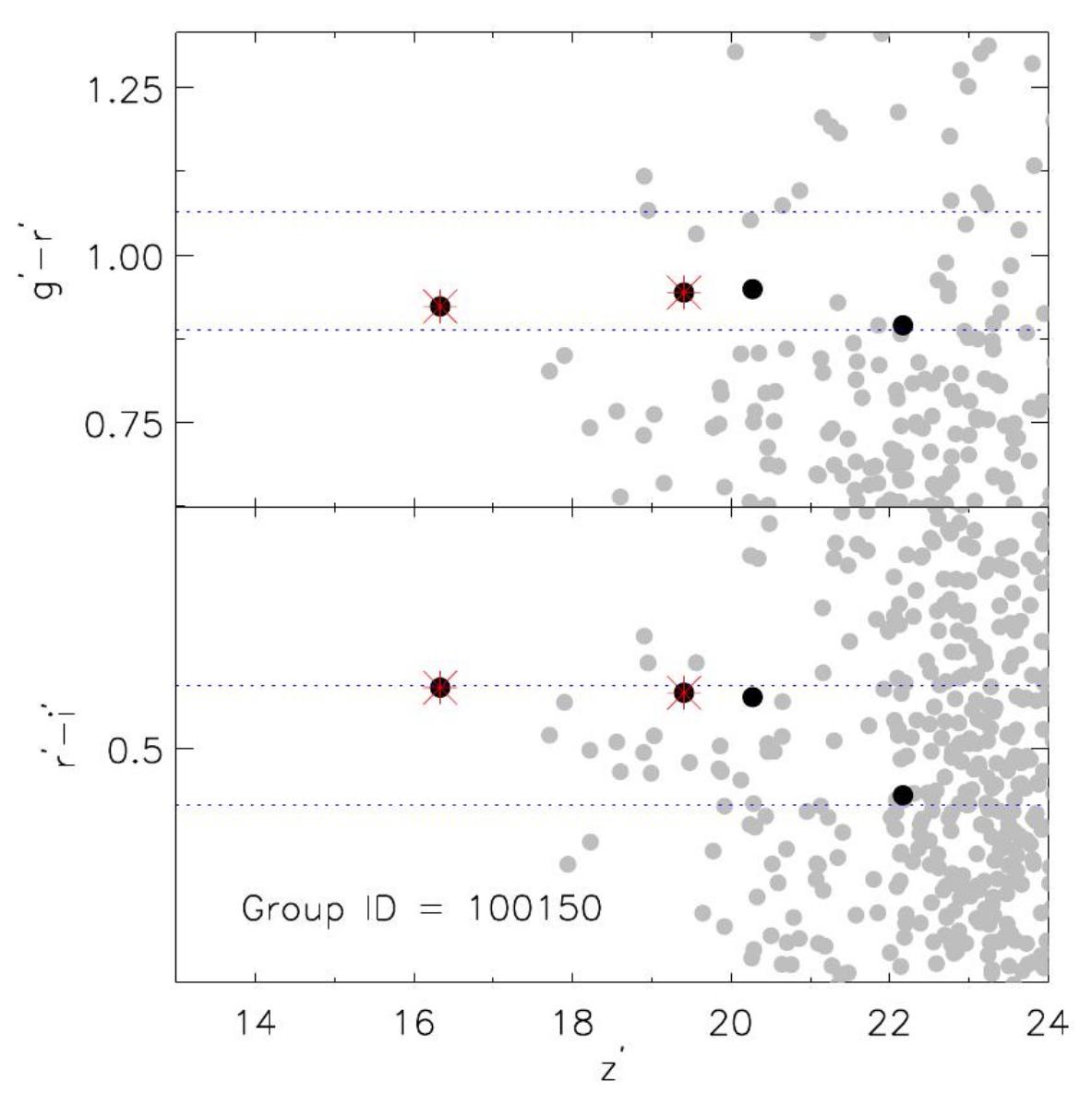
Figure 29: Same as in Fig. 23, but for the group100150 at z= 0.16.

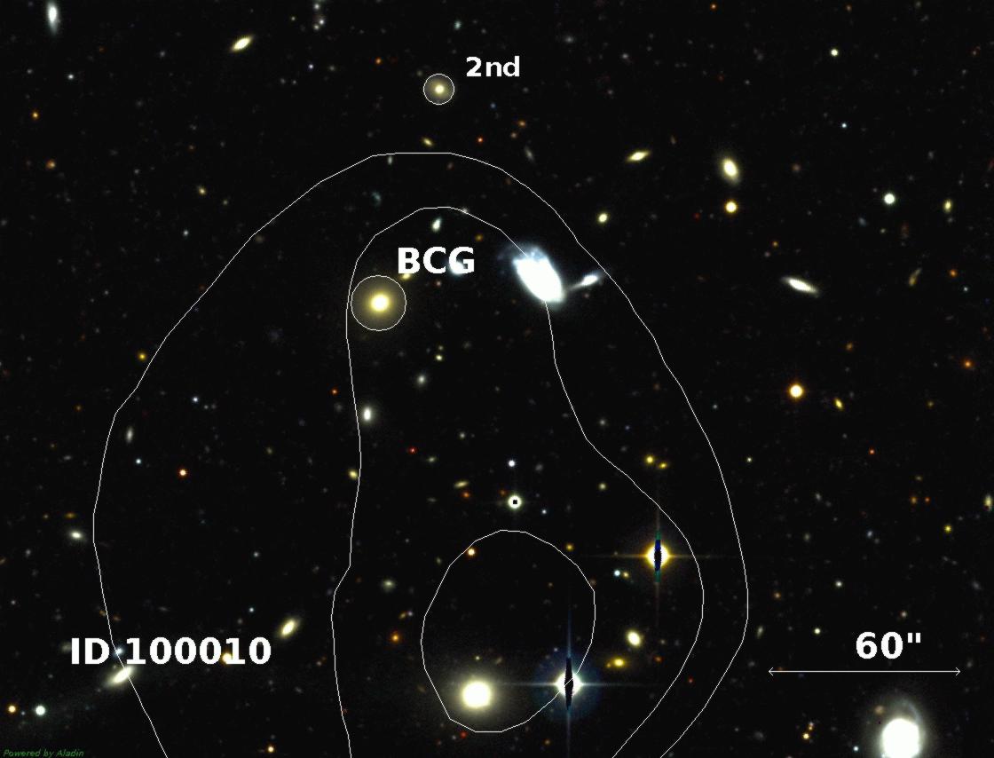
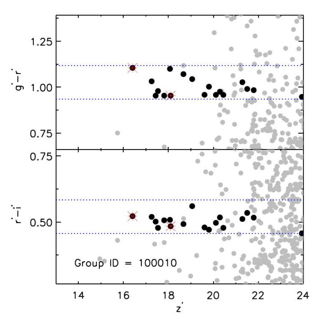
Figure 30: Same as in Fig. 23, but for the group 100010, at z=0.22.

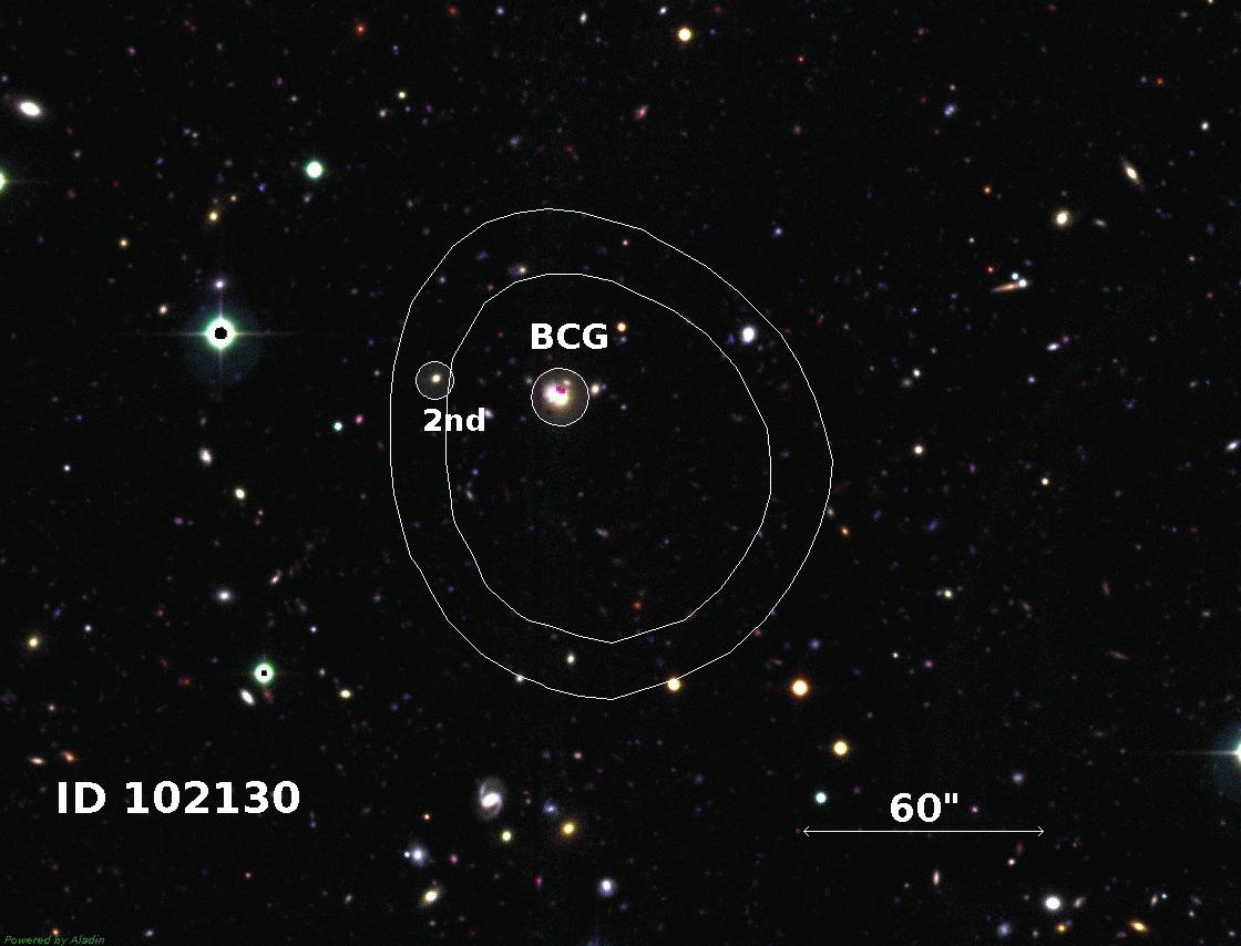
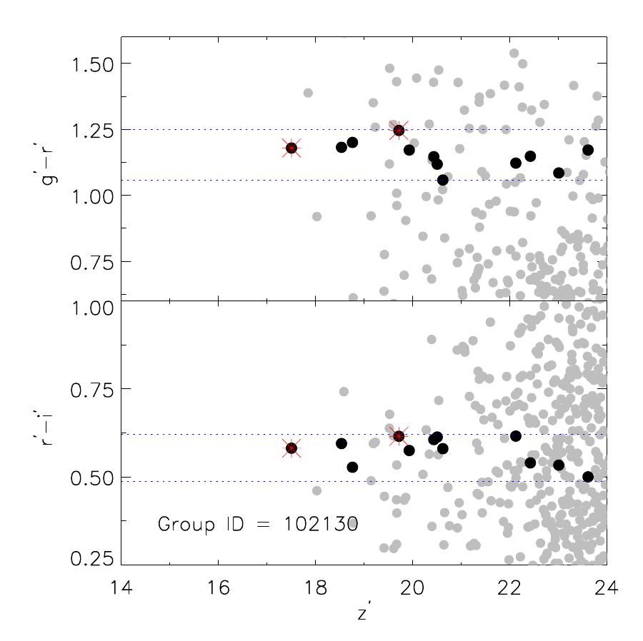
Figure 31: Same as in Fig. 23, but for the group 102130 at z=0.23.

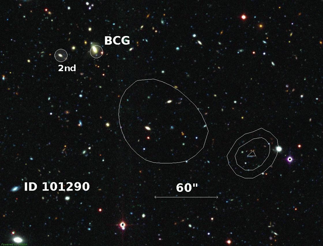
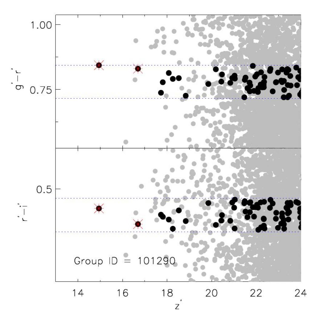
Figure 32: Same as in Fig. 23, but for the group 101290 at z=0.25.

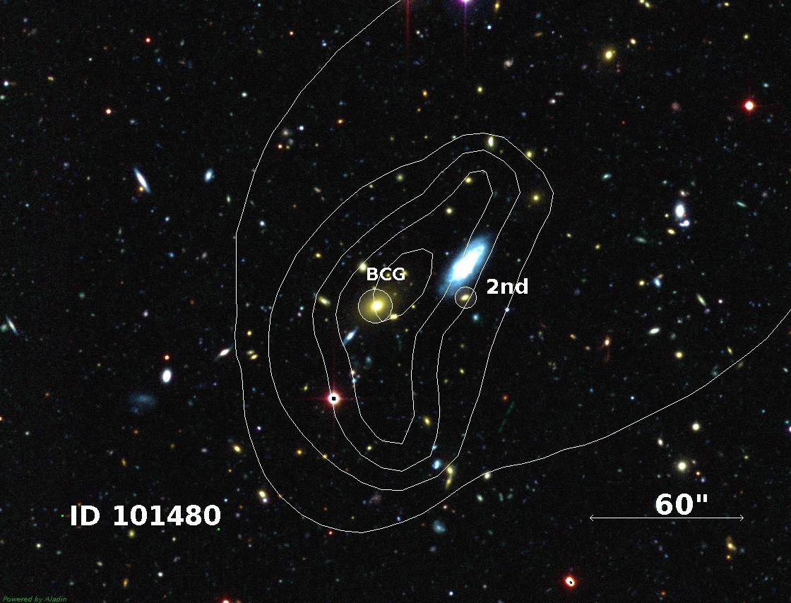
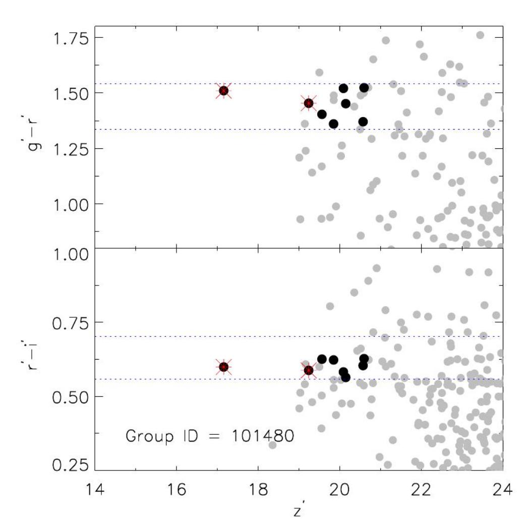
Figure 33: Same as in Fig. 23, but for the group 101480, at z=0.34.

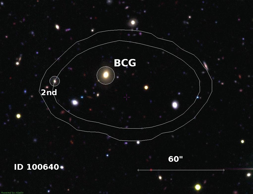
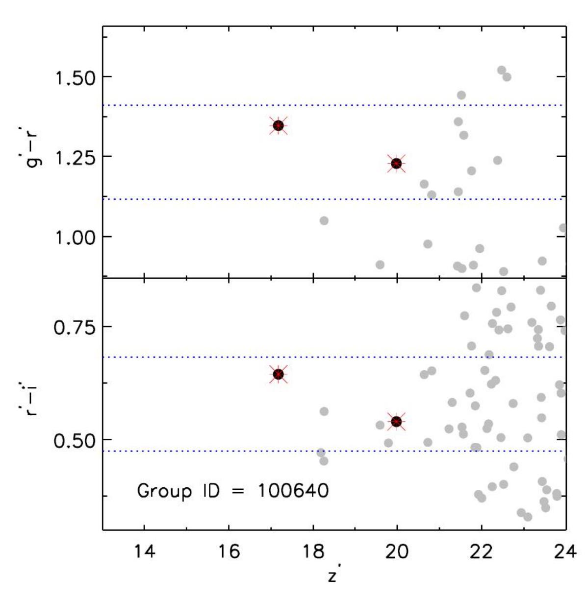
Figure 34: Same as in Fig. 23, but for the group 100640, at z=0.34.

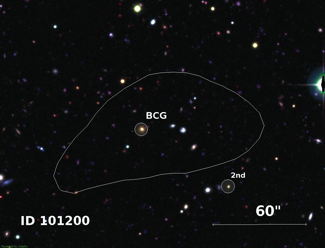
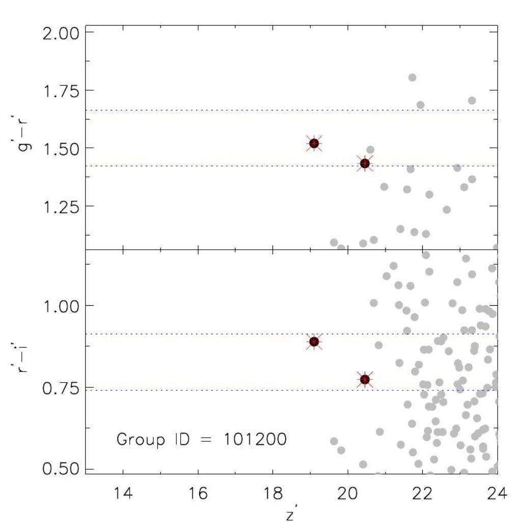
Figure 35: Same as in Fig. 23, but for the group 101200 at z=0.47. The 2-nd brightest galaxy cannot be found inside 0.5R₂₀₀ due to completeness effect and the marked galaxy is at 0.6R₂₀₀ distance to the center.

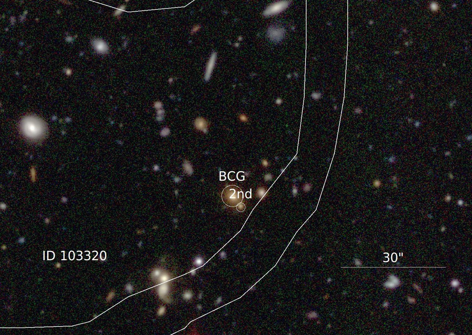
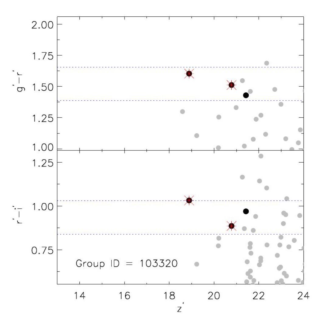
Figure 36: Same as in Fig. 23, but for the group 103320 at z=0.53.

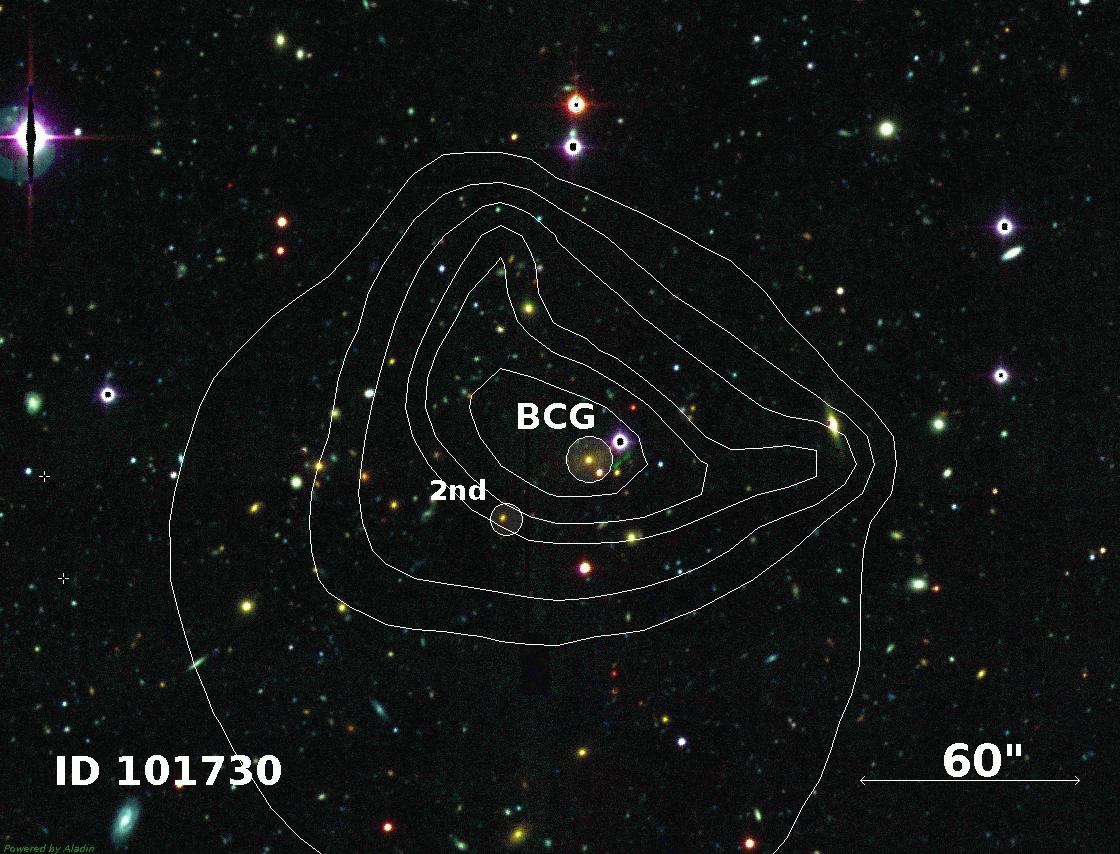
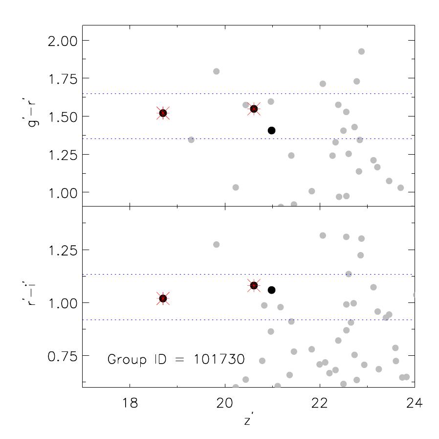
Figure 37: Same as in Fig. 23, but for the group 101730, at z 0.60.

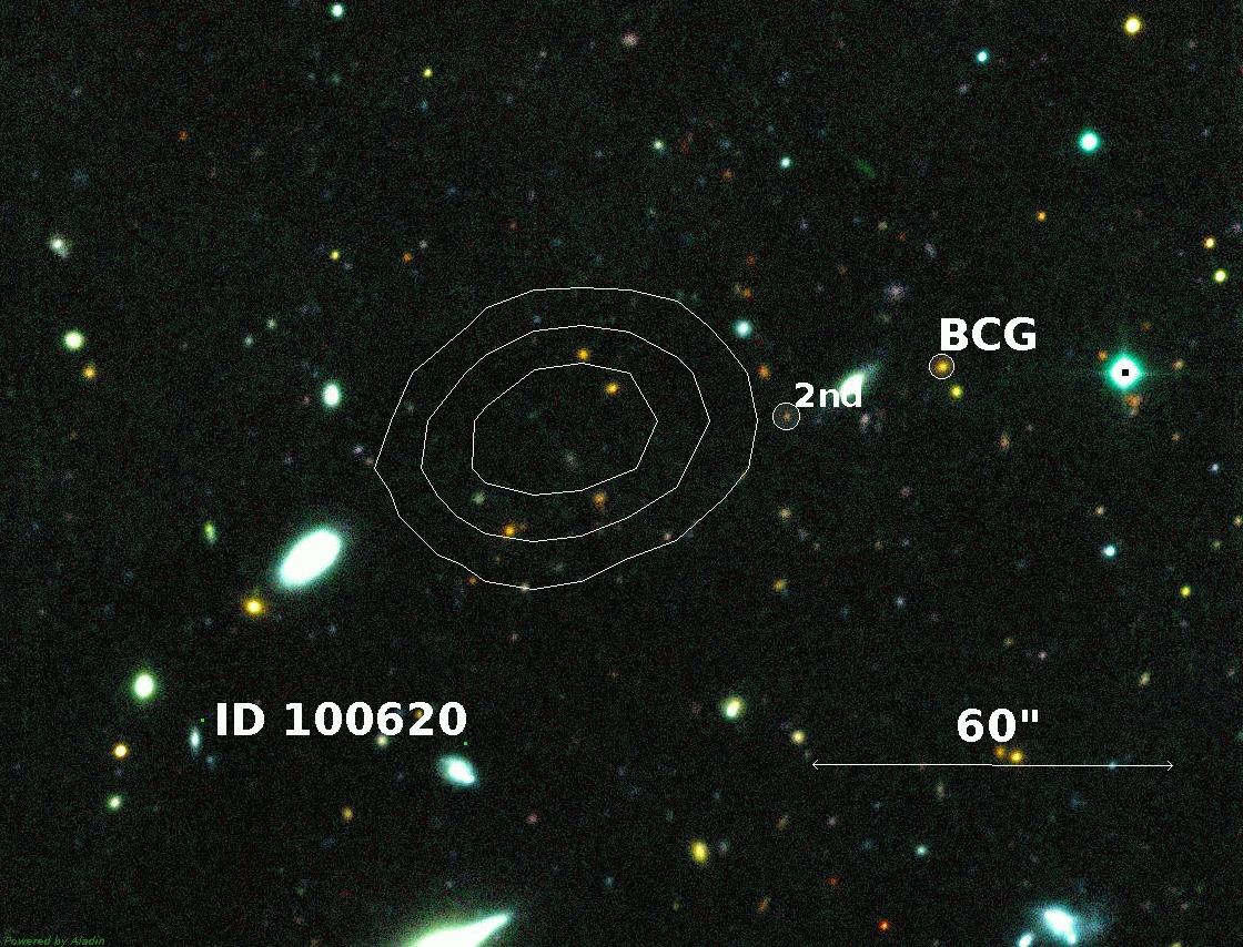
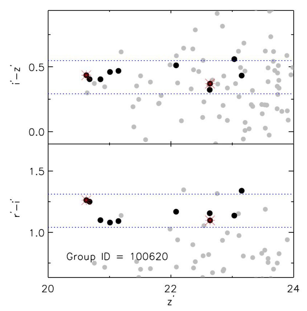
Figure 38: Upper panel. Contours of extended X-ray emission overlaid on the CFHTLS RGB image of the fossil group 100620 at z=0.66. Middle panel. i^′- z^′ versus z^′. Lower panel. r^′ - i^′ versus z^′. Filled black circles illustrate group members selected by the method described in §4.1. The BGG and second brightest satellite galaxy within $0.5R_{200}$ have been marked with red asterisks within each color magnitude diagram. The upper and lower limits of colors have been shown by horizontal dotted blue lines.

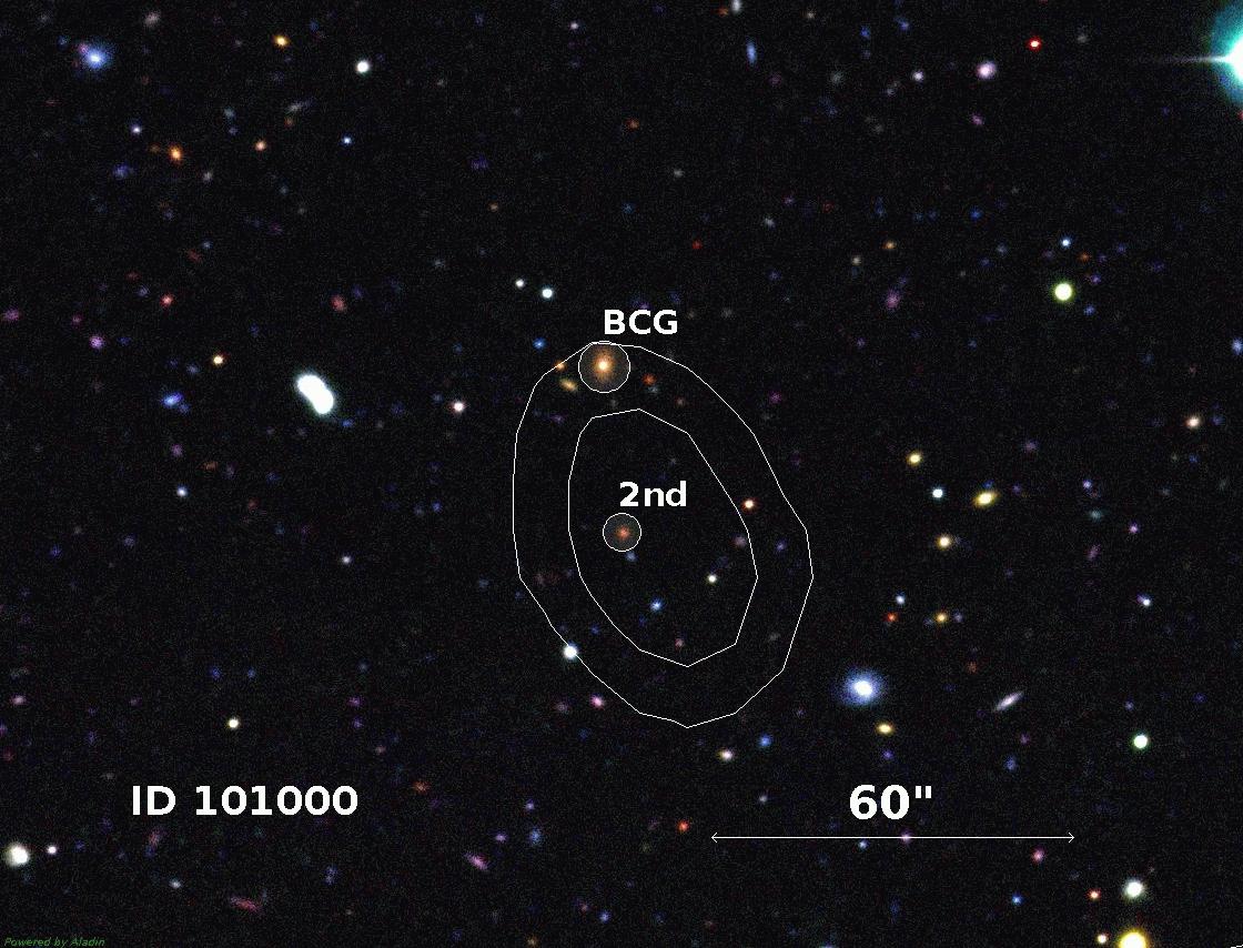
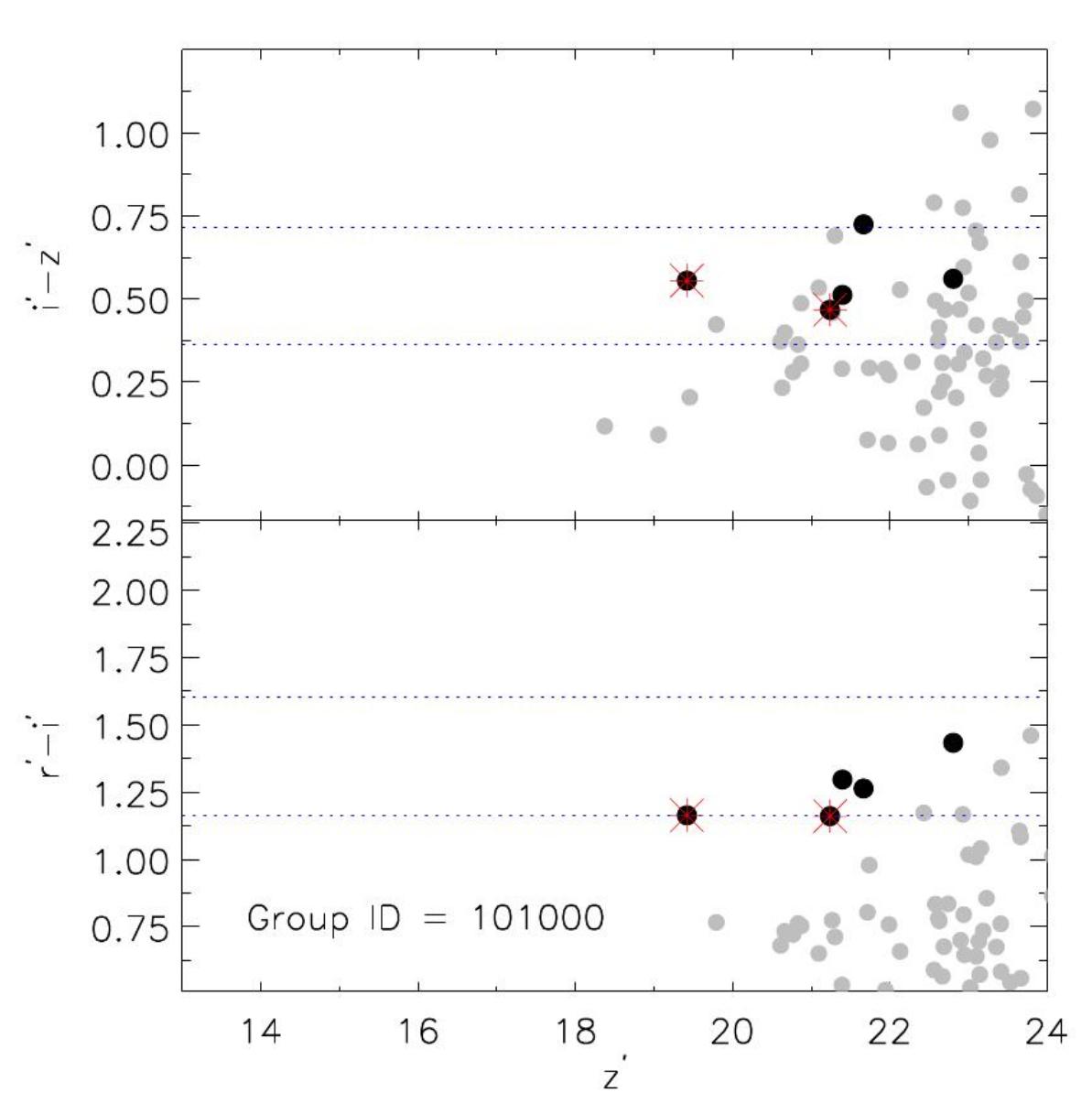
Figure 39: Same as in Fig. 38, but for the group 101000 at z=0.76.

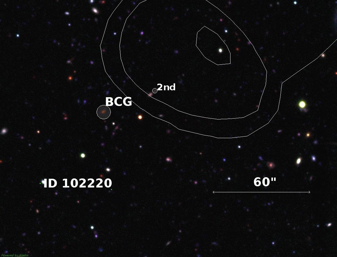
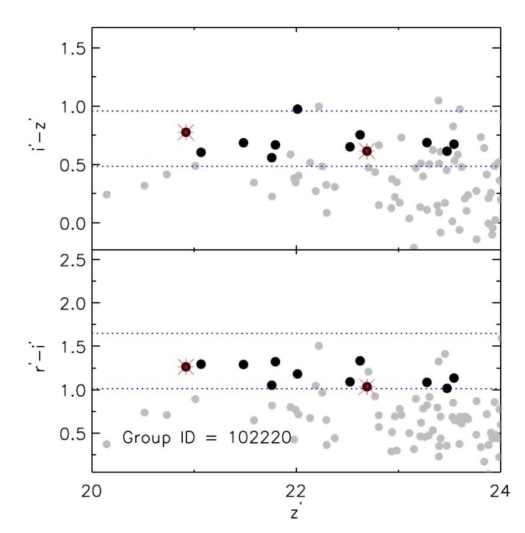
Figure 40: Same as in Fig. 38, but for the group 101120 at z=0.86.

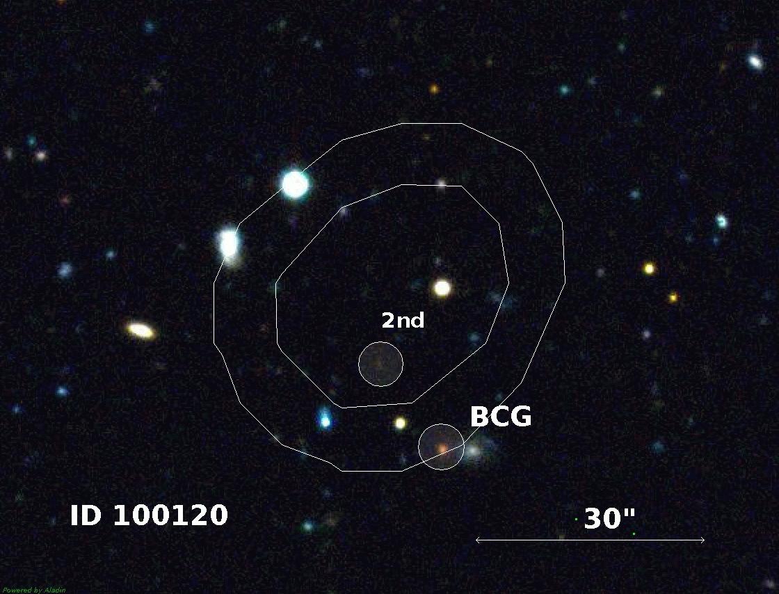
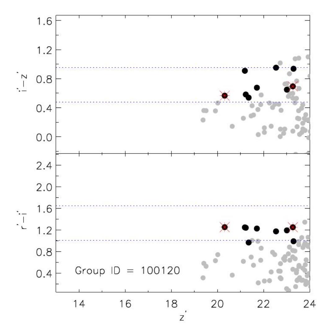
Figure 41: Same as in Fig. 38, but for the group 100120 at z=0.88.

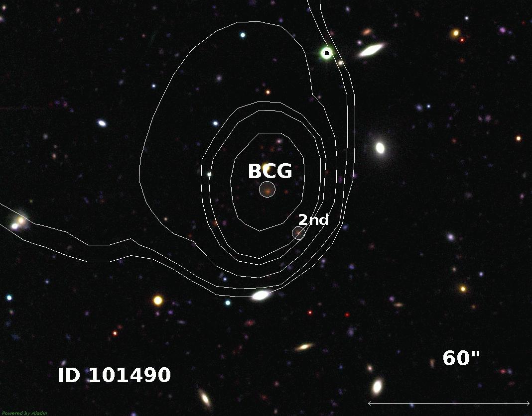
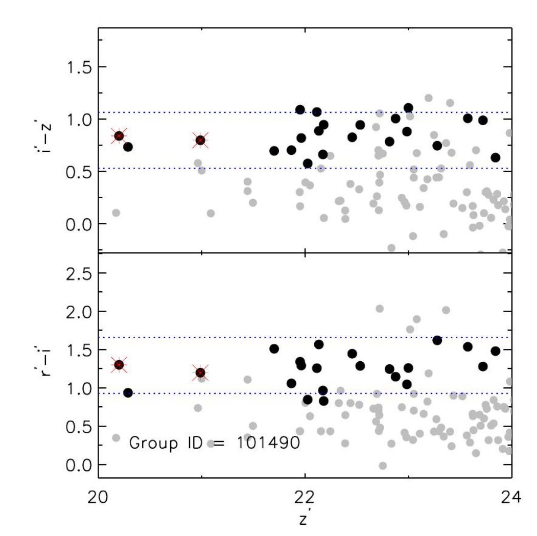
Figure 42: Same as in Fig. 38, but for the group 101490, at z=0.94.

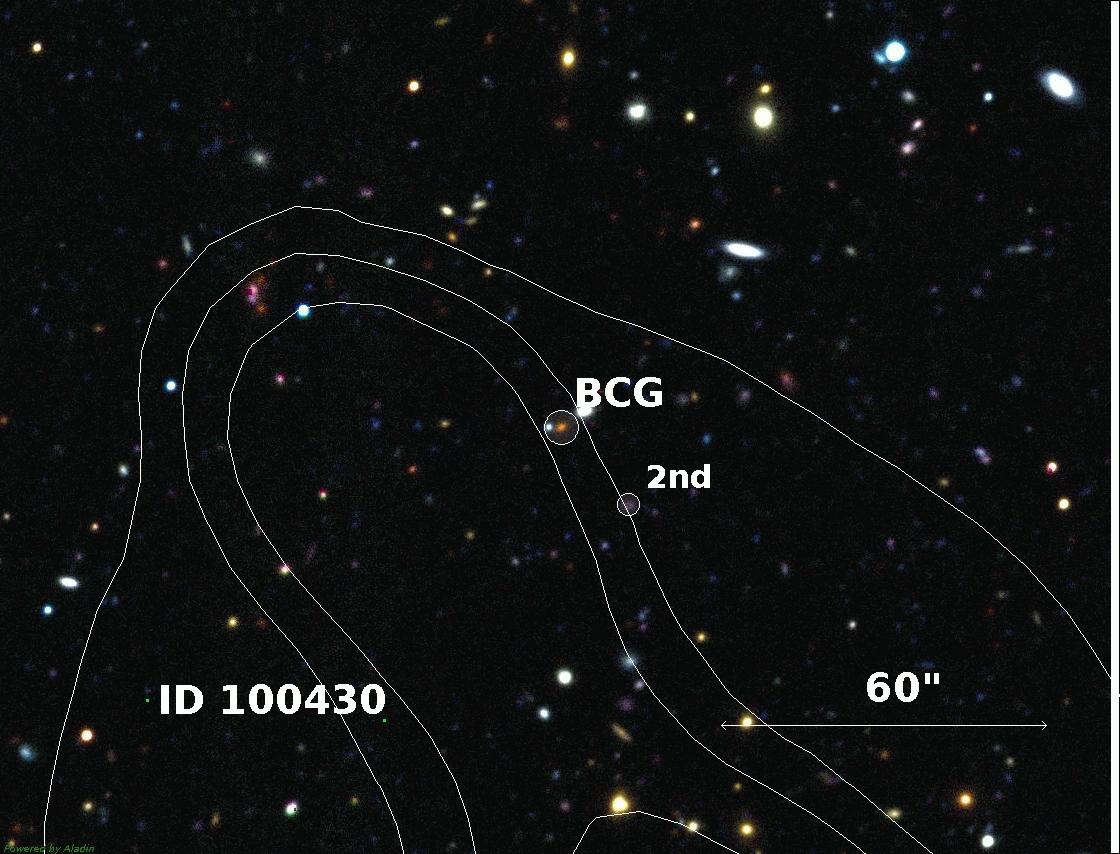
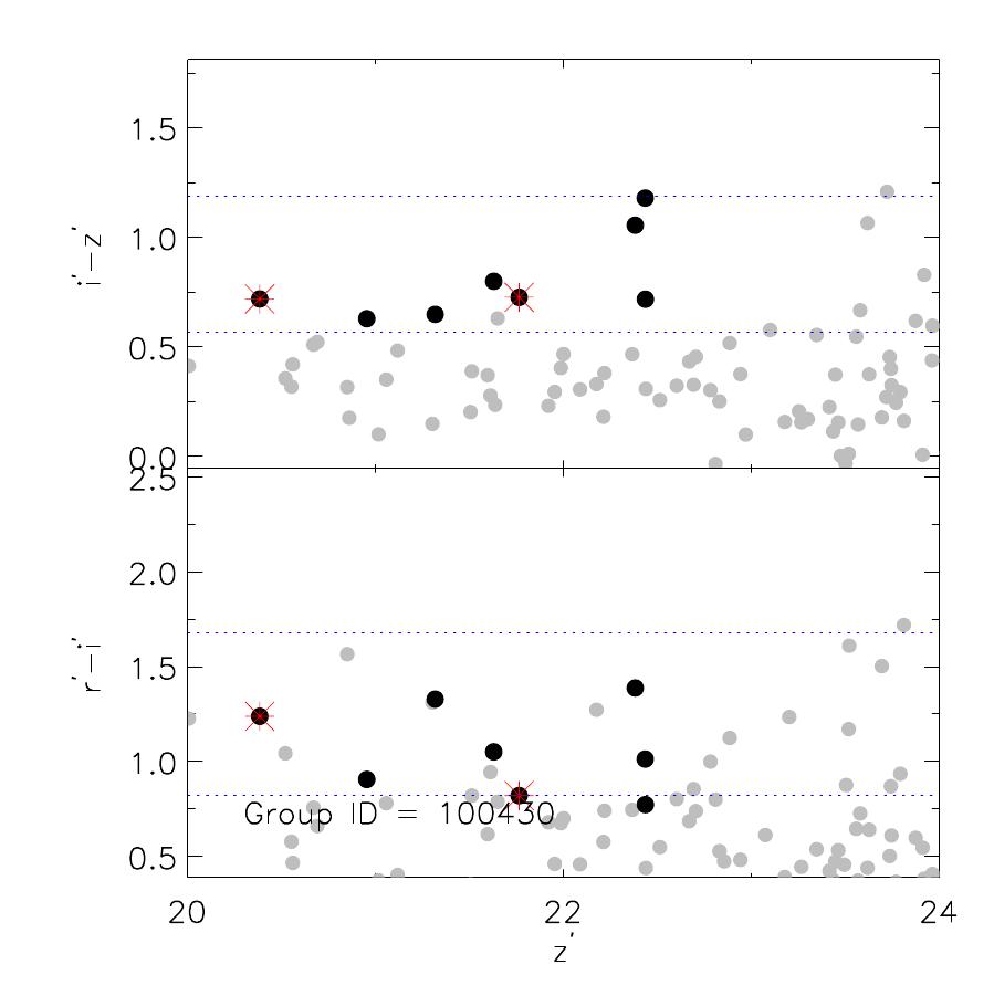
Figure 43: Same as in Fig. 38, but for the group 100430, at z=0.98.

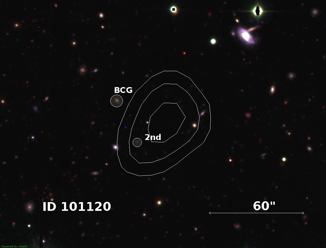
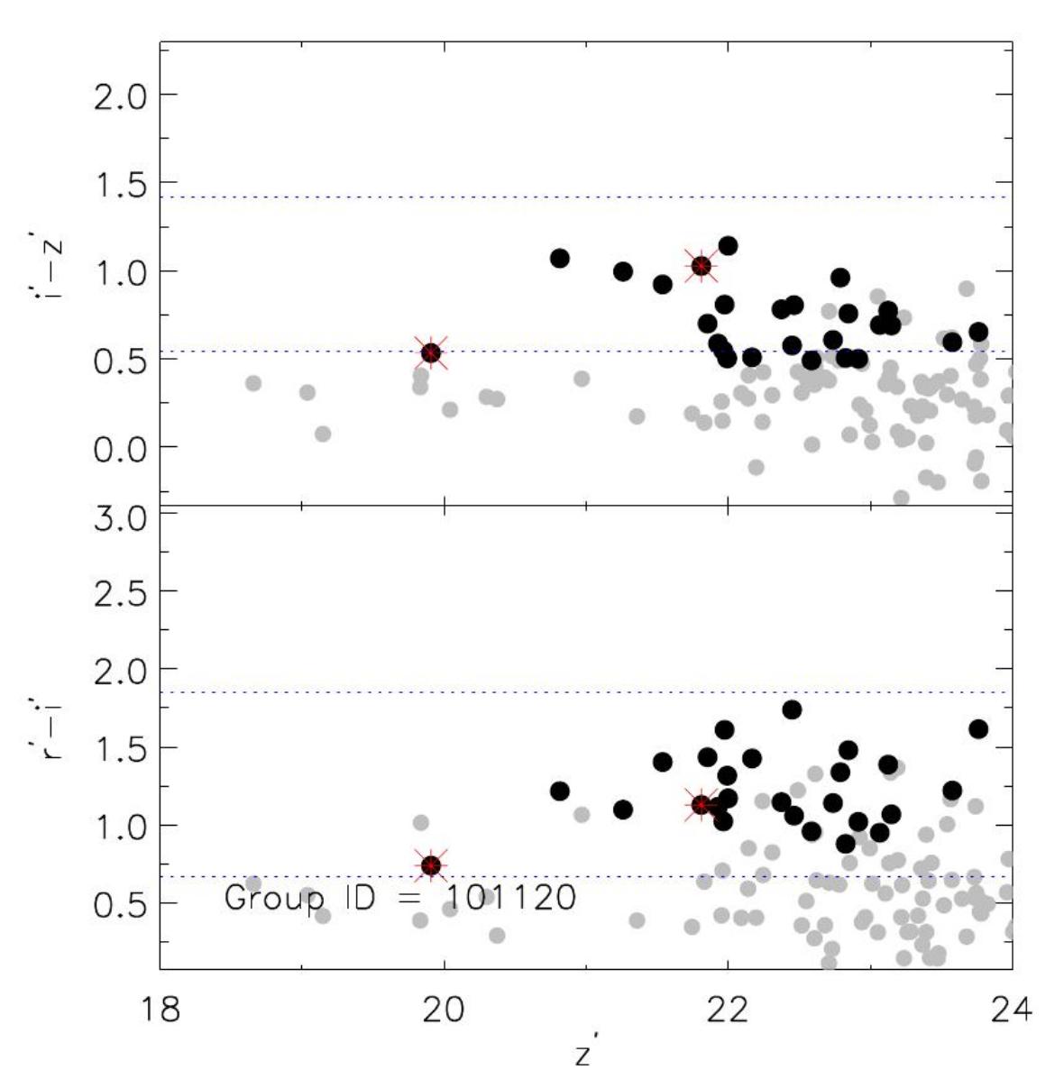
Figure 44: Same as in Fig. 38, but for the group 101120, at z=1.1.

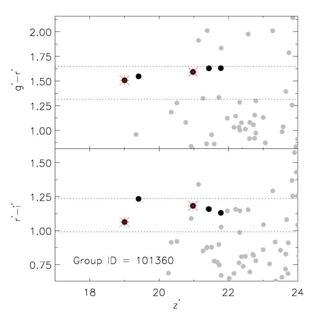
Figure 45: Same as in Fig. 23, but for the group 101360, at z= 0.60. The RGB image of this group has been presented in Fig. 6 (left bottom panel).

References

- Adami et al. (2011) Adami, C., Mazure, A., Pierre, M., et al. 2011, A&A, 526, A18
- Aihara et al. (2011) Aihara, H., Allende, P. C., An, D. & et al. 2011, ApJS, 193, 29
- Allevato et al. (2012) Allevato, V., Finoguenov, A., Hasinger, G., Miyaji, T., et al. 2012, ApJ, 758, 47
- Arnouts et al. (2002) Arnouts, S., et al. 2002, MNRAS, 329, 355
- Barnes (1989) Barnes, J. E. 1989, Nature, 338, 123
- Bauer et al. (2002) Bauer, F. E., et al. 2002, AJ, 123, 1163
- Benson et al. (2003) Benson, A. J., Bower, R. G., Frenk, C. S., et al. 2003, ApJ, 599, 38
- Bekki et al. (2002) Bekki, K., Forbes, D. A., Beasley, M. A., & Couch, W. J. 2002, MNRAS, 335, 1176
- Bielby et al. (2010) Bielby, R. M., Finoguenov, A., Tanaka, M., et al. 2010, A&A, 523, A66
- Bruzual & Charlot (2003) Bruzual, G., & Charlot, S. 2003, MNRAS, 344, 1000
- Bielby et al. (2010) Bielby, R. M., Finoguenov, A., Tanaka, M., et al. 2010, A&A, 523, A66
- Brimioulle et al. (2008) Brimioulle, F., Lerchster, M., Seitz, S., Bender, R., & Snigula, J. 2008, arXiv:0811.3211
- Brimioulle et al. (2013) Brimioulle, F., Seitz, S., Lerchster, M., Seitz, S., Bender, R., Snigula, J. 2013, MNRAS, 432, 1046
- Bordoloi et al. (2012) Bordoloi, R., Lilly, S. J., Amara, A., et al. 2012, MNRAS, 421, 1671
- Borgani & Guzzo (2001) Borgani, S. & Guzzo, L. 2001, A&A, 409, 39
- Bower et al. (2006) Bower, R. G., Benson, A. J., Malbon, R., et al. 2006, MNRAS, 370, 645
- Calzetti et al. (2000) Calzetti, D., et al. 2000, ApJ, 533, 682
- Cole et al. (2000) Cole, S., Lacey, C. G., Baugh, C. M., & Frenk, C. S. 2000, MNRAS, 319, 168
- Chabrier (2003) Chabrier, G. 2003, PASP, 115, 763
- Colless et al. (2001) Colless, M., et al. 2001, MNRAS, 328, 1039
- Connelly et al. (2012) Connelly, J. L., Wilman, D. J., Finoguenov, A., Hou, A., et al. 2012, ApJ, 756, 139
- Conroy et al. (2007b) Conroy, C., Wechsler, R. H., & Kravtsov, A. V. 2007, ApJ, 668, 826
- Conroy et al. (2007a) Conroy, C., Ho, S., & White, M. 2007, MNRAS, 379, 1491
- Croton et al. (2006) Croton, D.J., Springel, V., White, S.D.M.,et al. 2006, MNRAS, 365, 11
- Dariush et al. (2007) Dariush, A. A., Khosroshahi, H. G., Ponman, T. J., Pearce, F., Raychaudhury, S., Hartley W. 2007, MNRAS, 382, 433
- Dariush et al. (2010) Dariush, A. A., Raychaudhury, S., Ponman, T. J.,Khosroshahi, H. G., et al. 2010, MNRAS,405, 1873
- Davis et al. (1985) Davis, M., Efstathiou, G., Frenk, C. S., White, S. D. M., 1985, ApJ, 292, 371
- De Lucia & Blaizot (2007) De Lucia, G., Blaizot, J. 2007, MNRAS, 375, 2
- De Lucia et al. (2006) De Lucia, G., Springel, V., White, S. D. M., Croton, D.Kauffmann, G. 2006, MNRAS, 366, 499
- Díaz-Giménez et al. (2011) Díaz-Giménez, E., Zandivarez, A., Proctor, R., Mendes de Oliveira, C., & Abramo, L. R. 2011, A&A, 527, A129
- D’Onghia et al. (2005) D’Onghia, E., Sommer-Larsen, J., Romeo, A. D., et al. 2005, ApJ, 630, L109
- Eigenthaler & Zeilinger (2013) Eigenthaler, P., & Zeilinger, W. W. 2013, A&A, 553, A99
- Erben et al. (2013) Erben, T., Hildebrandt, H., Miller, L., et al. 2013, MNRAS, 433, 2545
- Erfanianfar et al. (2013) Erfanianfar, G., Finoguenov, A., Tanaka, M., et al. 2013, ApJ, 765, 117
- Erfanianfar et al. (2014) Erfanianfar, G., Popesso, P., Finoguenov, A. et al. 2014, MNRAS, subm.
- Fioc & Rocca-Volmerange (1999) Fioc, M., & Rocca-Volmerange, B. 1999, arXiv:astro-ph/9912179
- Finoguenov et al. (2005) Finoguenov, A., Streblyanska, A., Hasinger, G., Hashimoto, Y., Szokoly, G. 2005, Adv. Space Res., 36, 710
- Finoguenov et al. (2007) Finoguenov, A., et al. 2007, ApJS, 172, 182
- Finoguenov et al. (2009) Finoguenov, A., Connelly, J. L., Parker, L. C., et al. 2009, ApJ, 704, 564
- Finoguenov et al. (2010) Finoguenov, A., et al. 2010, MNRAS, 403, 2063
- Font et al. (2008) Font, A. S., Bower, R. G., McCarthy, I. G., et al. 2008, MNRAS, 389, 1619
- George et al. (2011) George, M. R., Leauthaud, A., Bundy, K., et al. 2011, ApJ, 742, 125
- Giacconi et al. (2002) Giacconi, R., et al. 2002, ApJS, 139, 369
- Giodini et al. (2009) Giodini, S., et al. 2009, ApJ, 703, 982
- Guo et al. (2011) Guo, Q., White, S., Boylan-Kolchin, M., De Lucia, G., Kaumann, G., Lemson, G., Li C., Springel, V., Weinmann, S. 2011, MNRAS, 413, 101
- Harker et al. (2006) Harker, G., Cole, S., Helly, J., Frenk, C., & Jenkins, A. 2006, MNRAS, 367, 1039
- Hearin et al. (2013) Hearin, A. P., Zentner, A. R.,Berlind, A. A., Newman, J. A. 2013, MNRAS, 433, 659
- Henriques & Thomas (2010) Henriques, B. M. B., & Thomas, P. A. 2010, MNRAS, 403, 768
- Humphrey et al. (2012) Humphrey, P. J., Buote, D. A., Brighenti, F., et al. 2012, ApJ, 748, 11H
- Huntley (1980) Huntley, J. M. 1980, ApJ, 238, 524
- Ilbert et al. (2009) Ilbert, O., Capak, P., Salvato, M., et al. 2009, ApJ, 690, 1236
- Ilbert et al. (2006) Ilbert, O., Arnouts, S., McCracken, H. J., et al. 2006, A&A, 457, 841
- Jansen et al. (2001) Jansen, F.; Lumb, D.; Altieri, B., et al 2001, A&A, 365, L1
- Jones et al. (2003) Jones, L. R., Ponman, T. J., Horton, A., Babul, A., Ebeling, H., Burke , D. J. 2003, MNRAS, 343, 627
- Junqueira et al. (2013) Junqueira, T. C., Lépine, J. R. D., Braga, C. A. S., & Barros, D. A. 2013, A&A, 550, A91
- Kauffmann & Haehnelt (2000) Kauffmann, G., Haehnelt, M. 2000, MNRAS, 311, 576
- Kennicutt (1983) Kennicutt, R. C., Jr. 1983, ApJ, 272, 54
- Khosroshahi et al. (2006) Khosroshahi, H. G., Maughan, B.J., Ponman, T. J. & Jones, L. R. 2006, MNRAS, 369, 1211
- Khosroshahi et al. (2007) Khosroshahi, H. G., Ponman, T. J. & Jones, L. R. 2007, MNRAS, 377, 595
- Kim et al. (2009) Kim, H.-S., Baugh, C. M., Cole, S., Frenk, C. S., & Benson, A. J. 2009, MNRAS, 400, 1527
- La Barbera et al. (2012) La Barbera, F., Paolillo, M., De Filippis, E., de Carvalho, R. R. 2012, MNRAS, 422, 3010
- Leauthaud et al. (2010) Leauthaud, A., Finoguenov, A., Kneib, J.-P. et al. 2010, ApJ, 709, 97
- Le Fèvre et al. (2004) Le Fèvre, O., et al., 2004, A&A, 428, 1023
- Le Fèvre et al. (2005) Le Fèvre, O., et al. 2005, A&A, 439, 845
- Libeskind et al. (2006) Libeskind, N. I., Cole, S., Frenk, C. S., & Helly, J. C. 2006, MNRAS, 368, 1381
- Liu et al. (2010) Liu, L., Yang, X., Mo, H. J., van den Bosch, F. C., & Springel, V. 2010, ApJ, 712, 734
- Maraston et al. (2009) Maraston, C., Strömbäck, G., Thomas, D., Wake, D. A., Nichol, R. C. 2009, MNRAS, 394L, 107
- Milosavljević et al. (2006) Milosavljević M., Miller C. J., Furlanetto S. R., Cooray A. 2006, ApJ, 637, L9
- Mirkazemi et al. (2014) Mirkazemi, M., Finoguenov, A. Pereira, M. J., et al. 2014, ApJ, subm.
- Mo et al. (1998) Mo, H. J., Mao, S., & White, S. D. M. 1998, MNRAS, 295, 319
- Pacaud et al. (2006) Pacaud, F., Pierre, M., Refregier, A., et al. 2006, MNRAS, 372, 578
- Pacaud et al. (2007) Pacaud, F. et al., 2007, MNRAS, 382, 1289
- Papovich et al. (2010) Papovich, C., Momcheva, I., Willmer, C. N. A., et al. 2010, ApJ, 716, 1503
- Percival et al. (2010) Percival, W. J., Reid, B. A., Eisenstein, D. J., et al. 2010, MNRAS, 401, 2148
- Pierre et al. (2007) Pierre, M. et al. 2007, MNRAS, 382, 279
- Pierre et al. (2012) Pierre, M., Clerc, N., Maughan, B., et al. 2012, A&A, 540, A4
- Ponman et al. (1994) Ponman, T.J., Allan, D.J., Jones, L.R., Merrifield, M. & MacHardy, I.M. 1994 Nature,369, 462
- Press & Schechter (1974) Press, W. H., & Schechter, P. 1974, ApJ, 187, 425
- Rosati et al. (2002) Rosati, P., Borgani, S., Norman, C. 2002, ARA&A, 40, 539
- Salvato et al. (2009) Salvato, M., Hasinger, G., Ilbert, O., et al. 2009, ApJ, 690, 1250
- Scoville et al. (2007) Scoville, N., Aussel, H., Brusa, M., Capak, P., et al. 2007, ApJS, 172, 1
- Silverman et al. (2009) Silverman, J. D. et al. 2009, ApJ, 695, 171
- Smith et al. (2010) Smith, G. P., Khosroshahi, H. G., Dariush, A., et al.2010, MNRAS, 409, 169
- Springel et al. (2001) Springel, V., Yoshida, N. & White, S. D. M. 2001, NewA, 6, 79S
- Spergel et al. (2003) Spergel, D. N., Verde, L., Peiris, H. V., Komatsu, E., et al. 2003, ApJS, 148, 175
- Springel et al. (2005) Springel, V. et al. 2005, Natur, 435, 629
- Somerville et al. (2001) Somerville, R. S., Primack, J. R., & Faber, S. M. 2001, MNRAS, 320, 504
- Strüder et al. (2001) Strüder, L., Briel, U., Dennerl, K. et al. 2001, A&A, 365, 18
- Šuhada et al. (2012) Šuhada, R., et al. , 2012, A&A, 537 , A39
- Su et al. (2013) Su, Y., White, R. E., III, & Miller, E. D. 2013, ApJ, 775, 89
- Tanaka et al. (2008) Tanaka, M., et al. 2008, A&A, 489, 571
- Tanaka et al. (2010) Tanaka, M., Finoguenov, A., & Ueda, Y. 2010, ApJ, 716, L152
- Tanaka et al. (2012) Tanaka, M., et al. 2012, PASJ, 64,22
- Tavasoli et al. (2011) Tavasoli, S., Khosroshahi, H. G., Koohpaee, A., Rahmani, H., Ghanbari, J. 2011, PASP, 123, 1
- Turner et al. (2001) Turner, M. J. L., Abbey, A., Arnaud, M., et al. 2001, A&A, 365L, 27
- van den Bosch et al. (2007) van den Bosch, F.C., Yang, X., Mo, H.J., et al. 2007, MNRAS, 376, 841
- van den Bosch et al. (2013) van den Bosch, F. C., More, S., Cacciato, M., Mo, H., & Yang, X. 2013, MNRAS, 430, 725
- Voevodkin et al. (2010) Voevodkin, A., Borozdin, K., Heitmann, K., Habib, S., Vikhlinin, A., Mescheryakov, A., Hornstrup, A., Burenin, R. 2010, ApJ, 708, 1376
- Von Benda-Beckmann et al. (2008) Von Benda-Beckmann, et al. 2008, MNRAS, 386, 2345
- Weinberg (1972) Weinberg, S. 1972, pp. 688. ISBN 0-471-92567-5. Wiley-VCH , July 1972.
- White & Frenk (1991) White, S. D. M. & Frenk, C. S. 1991, ApJ, 379, 52
- White & Rees (1978) White, S. D. M., & Rees, M. J. 1978, MNRAS, 183, 341
- Yang et al. (2005) Yang, X., Mo, H. J., Jing, Y. P., & van den Bosch, F. C. 2005, MNRAS, 358, 217
- Yang et al. (2008) Yang, X., Mo, H., van den Bosch, F. 2008, ApJ, 676, 248
- Yang et al. (2009) Yang, X., Mo, H. J., & van den Bosch, F. C. 2009, ApJ, 695, 900
- Zandivarez et al. (2006) Zandivarez, A., Martínez, H. J., & Merchán, M. E. 2006, ApJ, 650, 137
- Zel’dovich (1970) Zel’dovich, Y. B. 1970, A&A, 5, 84
- Zibetti et al. (2009) Zibetti, S., Pierini, D., Pratt, G. W. 2009, MNRAS, 392, 525