Probability and Statistics for Particle Physicists

Abstract

A pedagogical selection of topics in probability and statistics is presented. Choice and emphasis are driven by the author’s personal experience, predominantly in the context of physics analyses using experimental data from high-energy physics detectors.

0.1 Introduction

These notes are based on a series of three lectures on probability and statistics, given at the AEPSHEP 2012 physics school. While most of the attendance was composed of PhD students, it also included Master students and young post-docs; in consequence, a variable level of familiarity with the topics discussed was implicit. For consistency, the scope of the lectures spanned from very general concepts up to more advanced, recent developments. The first lecture reviewed basic concepts in probability and statistics; the second lecture focussed on maximum likelihood and multivariate techniques for statistical analysis of experimental data; the third and last lecture covered topics on hypothesis-testing and interval estimation. Whenever possible, the notation aligns with common usage in experimental high-energy physics (HEP), and the discussion is illustrated with examples related to recent physics results, mostly from the $B$-factories and the LHC experiments.

0.2 Basic concepts in probability and statistics

Mathematical probability is an abstract axiomatic concept, and probability theory is the conceptual framework to assess the knowledge of random processes. A detailed discussion of its development and formalism lies outside the scope of these notes. Other than standard classic books, like [1], there are excellent references available, often written by (high-energy) physicists, and well-suited for the needs of physicists. A non-comprehensive list includes [2, 3, 4, 5], and can guide the reader into more advanced topics. The sections on statistics and probability in the PDG [6] are also a useful reference; often also, the large experimental collaborations have (internal) forums and working groups, with many useful links and references.

0.2.1 Random processes

For a process to be called random, two main conditions are required: its outcome cannot be predicted with complete certainty, and if the process is repeated under the very same conditions, the new resulting outcomes can be different each time. In the context of experimental particle physics, such an outcome could be “a collision”, or “a decay”. In practice, the sources of uncertainty leading to random processes can be

• due to reducible measurement errors, i.e. practical limitations that can in principle be overcome by means of higher-performance instruments or improved control of experimental conditions;

• due to quasi-irreducible random measurement errors, i.e. thermal effects;

• fundamental, if the underlying physics is intrinsically uncertain, i.e. quantum mechanics is not a deterministic theory.

Obviously in particle physics, all three kinds of uncertainties are at play. A key feature of collider physics is that events resulting from particle collisions are independent of each other, and provide a quasi-perfect laboratory of quantum-mechanical probability processes. Similarly, unstable particles produced in HEP experiments obey quantum-mechanical decay probabilities.

0.2.2 Mathematical probability

Let $\Omega$ be the total universe of possible outcomes of a random process, and let $X,Y\dotsc$ be elements (or realizations) of $\Omega$; a set of such realizations is called a sample. A probability function ${\cal P}$ is defined as a map onto the real numbers:

$${\cal P}:\left\{\Omega\right\} \rightarrow \left[0:1\right]\ ,$$

$$X \rightarrow {\cal P}(X)\ .$$ (1)

This mapping must satisfy the following axioms:

$${\cal P}(\Omega) = 1\ ,$$

$${\rm if}\ X\cap Y = \oslash\ ,\ {\rm then}\ {\cal P}(X\cup Y)={\cal P}(X)+{\cal P}(Y)\ ,$$ (2)

from which various useful properties can be easily derived, i.e.

$${\cal P}(\overline{X}) = 1-{\cal P}(X)\ ,$$

$${\cal P}(X\cup\overline{X}) = 1\ ,$$

$${\cal P}(\oslash) = 1-{\cal P}(\Omega)=0\ ,$$

$${\cal P}(X\cup Y) = {\cal P}(X)+{\cal P}(Y)-{\cal P}(X\cap Y)\ ,$$ (3)

(where $\overline{X}$ is the complement of $X$). Two elements $X$ and $Y$ are said to the independent (that is, their realizations are not linked in any way) if

$${\cal P}(X\cap Y)={\cal P}(X){\cal P}(Y).$$ (4)

Conditional probability and Bayes’ theorem

Conditional probability ${\cal P}(X\mid Y)$ is defined as the probability of $X$, given $Y$. The simplest example of conditional probability is for independent outcomes: from the definition of independence in Eq. (4), it follows that if $X$ and $Y$ are actually independent, the condition

$${\cal P}(X\mid Y)={\cal P}(X)$$ (5)

is satisfied. The general case is given by Bayes’ theorem: in view of the relation ${\cal P}(X\cap Y)={\cal P}(Y\cap X)$, it follows that

$${\cal P}(X\mid Y)=\frac{{\cal P}(Y\mid X){\cal P}(X)}{{\cal P}(Y)}\ .$$ (6)

An useful corollary follows as consequence of Bayes’ theorem: if $\Omega$ can be divided into a number of disjoint subsets $X_{i}$ (this division process is called a partition), then

$${\cal P}(X\mid Y)=\frac{{\cal P}(Y\mid X){\cal P}(X)}{\sum_{i}{\cal P}(Y\mid X_{i}){\cal P}(X_{i})}\ .$$ (7)

The probability density function

In the context of these lectures, the relevant scenario is when the outcome of a random process can be stated in numerical form (i.e. it corresponds to a measurement): then to each element $X$ (which for HEP-oriented notation purposes, it is preferable to design as an event) corresponds a variable $x$ (that can be real or integer). For continuous $x$, its probability density function (PDF) $P(x)$ is defined as

$${\cal P}(X\ {\rm found}\ {\rm in}\ \left[x,x+dx\right])\ =\ P(x)dx\ ,$$ (8)

where $P(x)$ is positive-defined for all values of $x$, and satisfies the normalization condition

$$\int_{-\infty}^{+\infty}dx^{\prime}P(x^{\prime})\ =\ 1\ .$$ (9)

For a discrete $x_{i}$, the above definition can be adapted in a straightworward way:

$${\cal P}(X\ {\rm found}\ {\rm in}\ x_{i})\ =\ p_{i}\ ,$$

$${\rm with}\ \sum_{j}p_{j}=1\ {\rm and}\ p_{k}\geq 0\ \forall k\ .$$ (10)

Finite probabilities are obtained by integration over a non-infinitesimal range. It is sometimes convenient to refer to the cumulative density function (CDF) :

$$C(x)\ =\ \int_{-\infty}^{x}dx^{\prime}P(x^{\prime})\ ,$$ (11)

so that finite probabilities can be obtained by evaluating the CDF on the boundaries of the range of interest :

$${\cal P}(a<X<b)\ =\ C(b)-C(a)\ =\ \int_{a}^{b}dx^{\prime}P(x^{\prime})\ .$$ (12)

Other than the conditions of normalization Eq. (9) and positive-defined (or more precisely, to have a compact support, which implies that the PDF must become vanishingly small outside of some finite boundary) the PDFs can be arbitrary otherwise, and exhibit one or several local maxima or local minima. In contrast, the CDF is a monotonically increasing function of $x$, as shown on Figure 1, where a generic PDF and its corresponding CDF are represented.

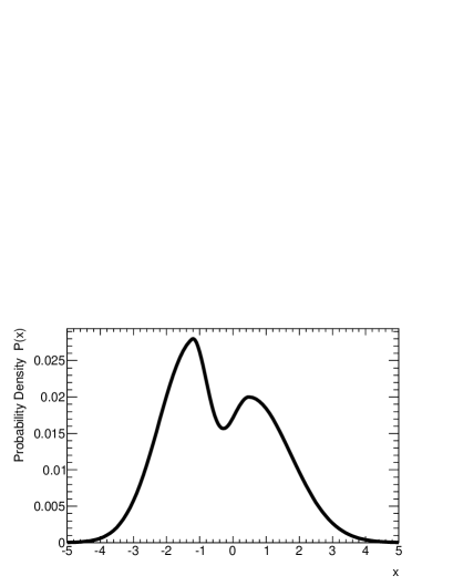
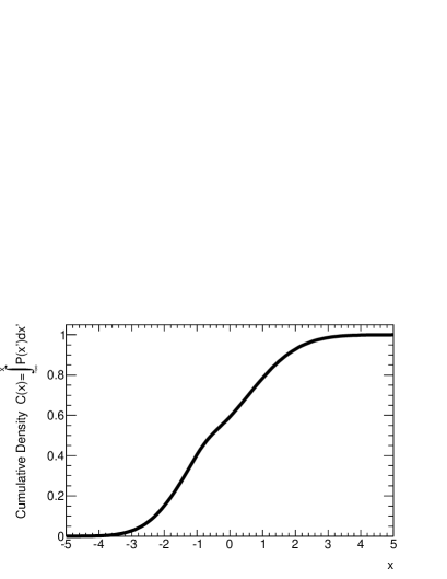
Figure 1: Left: a probability density function (PDF) for a variable $x$; the PDF is assumed to have negligible values outside of the plotted range. Right: the corresponding cumulative density function (CDF), plotted in the same range.

Multidimensional PDFs

When more than on random number is produced as outcome in a same event, it is convenient to introduce a $n$-dimensional set of random elements $\vec{X}=\left\{X_{1},X_{2},\dotsc,X_{n}\right\}$, together with its corresponding set of random variables $\vec{x}=\left\{x_{1},x_{2},\dotsc,x_{n}\right\}$ and their multidimensional PDF:

$$P(\vec{x})d\vec{x}\ =\ P(x_{1},x_{2},\dotsc,x_{n})dx_{1}dx_{2}\dotsc dx_{n}\ .$$ (13)

Lower-dimensional PDFs can be derived from Eq. (13); for instance, when one specific variable $x=x_{j}$ (for fixed $j$, with $1\leq j\leq n$) is of particlar relevance, its one-dimensional marginal probability density $P_{X}(x)$ is extracted by integrating $P(\vec{x})$ over the remaining $n-1$ dimensions (excluding the $j$-th):

$$P_{X}(x)dx=dx\int_{-\infty}^{+\infty}dx_{1}\dotsc\int_{-\infty}^{+\infty}dx_{j-1}\int_{-\infty}^{+\infty}dx_{j+1}\dotsc\int_{-\infty}^{+\infty}dy_{n-1}\ .$$ (14)

Without loss of generality, the discussion can be restricted to the two-dimensional case, with random elements $X$ and $Y$ and random variables $\vec{X}=\left\{x,y\right\}$. The finite probability in a rectangular two-dimensional range is

$${\cal P}(a<X<b\ {\rm and}\ c<Y<d)\ =\ \int_{a}^{b}dx\int_{c}^{d}dyP(x,y)\ .$$ (15)

For a fixed value of $Y$, the conditional density function for $X$ is given by

$$P(x\mid y)=\frac{P(x,y)}{\int dyP(x,y)}=\frac{P(x,y)}{P_{Y}(y)}\ .$$ (16)

As already mentioned, the relation $P(x,y)=P_{X}(x)\cdot P_{Y}(y)$ holds only if $X$ and $Y$ are independent; for instance, the two-dimensional density function in Figure 2 is an example of non-independent variables, for which $P(x,y)\neq P_{X}(x)\cdot P_{Y}(y)$.

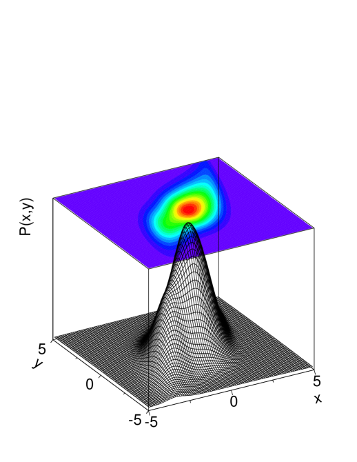
Figure 2: A two-dimensional probability density function (PDF) for non-independent variables $x$ and $y$: the pattern implies that in general, the probability densities are larger when $x$ and $y$ are both large or both small (i.e. they are positively correlated), and thus the variables are not independent. The PDF is assumed to have negligible values outside of the plotted two-dimensional range.

0.3 Parametric PDFs and parameter estimation

The description of a random process via density functions is called a model. Loosely speaking, a parametric model assumes that its PDFs can be completely described using a finite number of parameters . A straightforward implementation of a parametric PDF is when its parameters are analytical arguments of the density function; the notation $P\left(x,y,\dotsc;\theta_{1},\theta_{2},\dotsc\right)$ indicates the functional dependence of the PDF (also called its shape) in terms of variables $x_{1},y_{2},\dotsc$ and parameters $\theta_{1},\theta_{2},\dotsc$.

0.3.1 Expectation values

Consider a random variable $X$ with PDF $P(x)$. For a generic function $f(x)$, its expectation value $E[f]$ is the PDF-weighted average over the $x$ range :

$$E[f]\ =\ \int dxP(x)f(x)\ .$$ (17)

Being often used, some common expectation values have their own names. For one-dimensional PDFs, the mean value and variance are defined as

$${\rm Mean\ value} :\ \mu\ = \ E[x]\ =\ \int dxP(x)x\ ,$$ (18)

$${\rm Variance} :\ \sigma^{2}\ = \ V[x]\ =\ E[x^{2}]-\mu^{2}\ =\ E[(x-\mu)^{2}]\ ;$$ (19)

for multidimensional PDFs, the covariance $C_{ij}=C(x_{i},x_{j})$ and the dimensionless linear correlation coefficient $\rho_{ij}$ are defined as:

$${\rm Covariance} :\ C_{ij}\ = \ E[x_{i}x_{j}]-\mu_{i}\mu_{j}\ =\ E[(x_{i}-\mu_{i})(x_{j}-\mu_{j})]\ ,$$ (20)

$${\rm Linear}\ {\rm correlation} :\ \rho_{ij}\ = \ \frac{C_{ij}}{\sigma_{i}\sigma_{j}}\ .$$ (21)

By construction, linear correlation coefficients have values in the $-1\leq\rho_{ij}\leq 1$ interval. The sign of the $\rho$ coefficient indicates the dominant trend in the $(x_{j};x_{j})$ pattern: for positive correlation, the probability density is larger when $x_{i}$ and $x_{j}$ are both small or large, while a negative correlation indicates that large values of $x_{i}$ are preferred when small values of $x_{j}$ are realized (and viceversa). When the random variables $X_{i}$ and $X_{j}$ are independent, that is $P(x_{i},x_{j})=P_{X_{i}}(x_{i})P_{X_{j}}(x_{j})$, one has

$$E[x_{i}x_{j}]\ =\ \int\int dx_{i}dx_{j}P(x_{i},x_{j})x_{i}x_{j}\ =\ \mu_{i}\mu_{j}\ ,$$ (22)

and thus $\rho_{ij}=0$: independent variables have a zero linear correlation coefficient. Note that the converse needs not be true: non-linear correlation patterns among non-independent variables may “conspire” and yield null values of the linear correlation coefficient, for instance if negative and positive correlation patterns in different regions of the $(x_{i},x_{j})$ plane cancel out. Figure 3 shows examples of two-dimensional samples, illustrating a few representative correlation patterns among their variables.

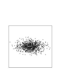
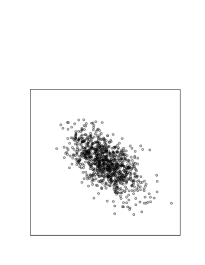
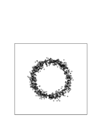
Figure 3: Examples of two-dimensional probability density functions, illustrating four typical correlation patterns. From left ro right, the figures show two variables which exhibit: a large, positive linear correlation (with $\rho=+0.9$); no correlation, with a zero linear correlation coefficient; a slightly milder, negative correlation (with $\rho=-0.5$); and a more complex correlation pattern, with variables very strongly correlated, but in such a way that the linear correlation coefficient is zero.

0.3.2 Shape characterisation

In practice, the true probability density function may not be known, and the accessible information can only be extracted from a finite-size sample (say consisting of $N$ events), which is assumed to have been originated from an unknown PDF. Assuming that this underlying PDF is parametric, a procedure to estimate its functional dependence and the values of its parameters is called a characterisation of its shape. Now, only a finite number of expectation values can be estimated from a finite-size sample. Therefore, when choosing the set of parameters to be estimated, each should provide information as useful and complementary as possible; such procedure, despite being intrinsically incomplete, can nevertheless prove quite powerful.

The procedure of shape characterisation is first illustrated with the one-dimensional case of a single random variable $x$. Consider the empirical average $\overline{x}$ (also called sample mean)

$$\overline{x}\ =\ \frac{1}{N}\sum_{i=1}^{N}x_{i}\ .$$ (23)

As shown later in Sec. 0.3.3, $\overline{x}$ is a good estimator of the mean value $\mu$ of the underlying distribution $P(x)$. In the same spirit, the quadratic sample mean (or root-mean-square RMS),

$${\rm RMS}\ =\ \sqrt{\overline{x^{2}}-\left(\overline{x}\right)^{2}}\ ,$$ (24)

is a reasonable estimator of its variance $\sigma^{2}$ (an improved estimator of variance can be easily derived from the RMS, as discussed later in Sec. 0.3.3). Intuitively speaking, these two estimators together provide complementary information on the “location” and “spread” of the region with highest event density in $x$.

The previous approach can be discussed in a more systematic way, by means of the characteristic function, which is a transformation from the $x$-dependence of the PDF $P(x)$ onto a $k$-dependence of $C[k]$, defined as

$$C[k]\ =\ E\left[e^{ik\frac{x-\mu}{\sigma}}\right]\ =\ \sum_{j}\frac{(ik)^{j}}{j!}\mu_{j}\ .$$ (25)

The coefficients $\mu$ of the expansion are called reduced moments; by construction, the first moments are $\mu_{1}=0$ and $\mu_{2}=1$; these values indicate that in terms of the rescaled variable $x^{\prime}=(x-\mu)/\sigma$, the PDF has been shifted to have zero mean and scaled to have unity variance.

In principle, the larger the number of momenta $\mu_{j}$ that are estimated, the more detailed is the characterisation of the PDF shape. Among higher-order moments, the third and fourth have specific names, and their values can be interpreted, in terms of shape, in a relatively straightforward manner. The third moment is called skewness: a symmetric distribution has zero skewness, and a negative (positive) value indicates a larger spread to the left (right) of its median. The fourth moment is called kurtosis; it is a positive-defined quantity, that (roughly speaking) can be related to the "peakedness" of a distribution: a large value indicates a sharp peak and long-range tails (such a distribution is sometimes called leptokurtic), while a smaller value reflects a broad central peak with short-range tails (a so-called platykurtic distribution). Figure 4 shows a few distributions, chosen to illustrate the relation of momenta and shapes.

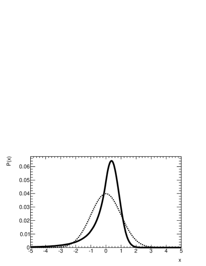
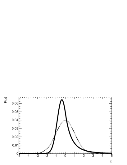
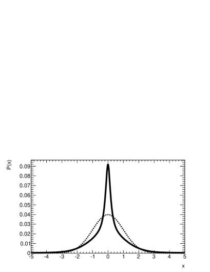
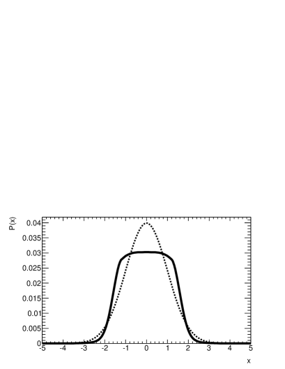
Figure 4: Examples of probability density functions, illustrating the role of momenta in the characterization of PDF shapes. For all PDFs plotted, their mean values are 0 and their variances are 1. Top plots : the PDF on the left (resp. right) exhibits an asymmetric, non-gaussian tail to the left (resp. right) of its peak, and thus has a positive (resp. negative) skewness. Bottm plots: the PDF on the left (resp. right) shows a narrow peak and long-range tails (resp. broad core and short-range tails), and has a large (resp. small) kurtosis. In each plot, a Gaussian PDF (dashed line) with mean value 0 and variance 1, is also overlaid.

0.3.3 Parameter estimation

The characterization of the shape of a PDF through a sequential estimation of shape parameters discussed in Sec. 0.3.2, aimed at a qualitative introduction to the concept of parameter estimation (also called point estimation in the litterature). A more general approach is now discussed in this paragraph.

Consider a $n$-dimensional, $k$-parametric PDF,

$$P(\ x_{1},x_{2},\dotsc,x_{n}\ ;\ \theta_{1},\theta_{2},\dotsc,\theta_{k}\ )\ ,$$ (26)

for which the values $\theta_{1},\dotsc,\theta_{k}$ are to be estimated on a finite-sized sample, by means of a set of estimators denoted $\hat{\theta_{1}},\dotsc,\hat{\theta_{k}}$. The estimators themselves are random variables, with their own mean values and variances: their values differ when estimated on different samples. The estimators should satisfy two key properties: to be consistent and unbaised. Consistency ensures that, in the infinite-sized sample limit, the estimator converges to the true parameter value; absence of bias ensures that the expectation value of the estimator is, for all sample sizes, the true parameter value. A biased, but consistent estimator (also called asymptotically unbiased) is such that the bias decreases with increasing sample size. Additional criteria can be used to characterize the quality and performance of estimators; two often mentioned are

• efficiency: an estimator with small variance is said to be more efficient than one with larger variance;

• robustness: this criterion characterizes the sensitivity of an estimator to uncertainties in the underlying PDF. For example, the mean value is robust against uncertainties on even-order moments, but is less robust with respect to changes on odd-order ones.

Note that these criteria may sometimes be mutually conflicting; for practical reasons, it may be preferable to use an efficient, biased estimator to an unbiased, but poorly convergent one.

The classical examples: mean value and variance

The convergence and bias requirements can be suitably illustrated with two classical, useful examples, often encountered an many practical situations: the mean value and the variance.

The empirical average $\overline{x}$ is a convergent, unbiased estimation of the mean value $\mu$ of its underlying distribution: $\hat{\mu}=\overline{x}$. This statement can easily be demostrated, by evaluating the expectation value and variance of $\overline{x}$:

$$E\left[\overline{x}\right] = \frac{1}{N}\sum_{i=1}^{N}E\left[x\right]\ =\ \mu\ ,$$ (27)

$$V\left[\overline{x}\right] = E\left[(\overline{x}-\mu)^{2}\right]\ =\ \frac{\sigma^{2}}{N}\ .$$ (28)

In contrast, the empirical RMS of a sample is a biased, asymptotically unbiased estimator of the variance $\sigma^{2}$: this can be demonstrated by first rewriting its square (also called sample variance) in terms of the mean value:

$${\rm RMS}^{2}\ =\ \frac{1}{N}\sum_{i=1}^{N}\left(x_{i}-\overline{x}\right)^{2}\ =\ \frac{1}{N}\sum_{i=1}^{N}\left(x_{i}-\mu\right)^{2}-\left(\overline{x}-\mu\right)^{2}\ ,$$ (29)

and so its expectation value is

$$E\left[{\rm RMS}^{2}\right]\ =\ \sigma^{2}-V\left[\overline{x}\right]\ =\ \frac{N-1}{N}\sigma^{2}\ ,$$ (30)

which, while properly converging to the true variance $\sigma^{2}$ in the $N\to\infty$ limit, systematically underestimates its value for a finite-sized sample. One can instead define a modified estimator

$$\frac{N}{N-1}{\rm RMS}^{2}\ =\ \frac{1}{N-1}\sum_{i=1}^{N}\left(x_{i}-\overline{x}\right)^{2}\ ,$$ (31)

that ensures, for finite-sized samples, an unbiased estimation of the variance.

In summary, consistent and unbiased estimators for the mean value $\mu$ and variance $\sigma^{2}$ of an unknown underlying PDF can be extracted from a finite-sized sample realized out of this PDF:

$$\hat{\mu} = \frac{1}{N}\sum_{i=1}^{N}x_{i}\ ,$$ (32)

$$\hat{\sigma}^{2} = \frac{1}{N-1}\sum_{i=1}^{N}\left(x_{i}-\hat{\mu}\right)^{2}\ .$$ (33)

As a side note, the $1/N$ and $1/(N-1)$ factors for $\hat{\mu}$ in Eq. (32) and for $\hat{\sigma}^{2}$ in Eq. (33) can be intuitively understood as follows: while the empirical average be estimated even on the smallest sample consisting of a single event, at least two events are needed to estimate their empirical dispersion.

Covariance, correlations, propagation of uncertainties

These two classical examples discussed in 0.3.3 refer to a single random variable. In presence of several random variables, expressed as a random $n$-dimensional vector $\vec{x}=\left\{x_{1},\dotsc,x_{n}\right\}$, the discussion leads to the definition of the empirical covariance matrix, whose elements $\hat{C}_{ab}$ can be estimated on a sample of $N$ events as

$$\hat{C}_{ab}\ =\ \frac{1}{N-1}\sum_{i=1}^{N}\left(x_{a,i}-\hat{\mu_{a}}\right)\left(x_{b,i}-\hat{\mu_{b}}\right)\ .$$ (34)

(the $a,b$ indices run over random variables, $1\leq a,b\leq n$). Assuming the covariance is known (i.e. by means of the estimator above, or from first principles), the variance of an arbitrary function of these random variables $f(\vec{x})$ can be evaluated from a Taylor-expansion around the mean values $\hat{\vec{\mu}}$ as

$$f\left(\vec{x}\right)\ =\ f\left(\hat{\vec{\mu}}\right)+\sum_{a=1}^{n}\left.\frac{df}{dx_{a}}\right|_{\vec{x}=\hat{\vec{\mu}}}\left(x_{a}-\hat{\mu}_{a}\right)\ ,$$ (35)

which leads to $E\left[f(\vec{x})\right]\ \simeq\ f(\hat{\vec{\mu}})$; similarly,

$$E\left[f^{2}(\vec{x})\right]\ \simeq\ f^{2}(\hat{\vec{\mu}})+\sum_{a,b=1}^{n}\left.\frac{df}{dx_{a}}\frac{df}{dx_{b}}\right|_{\vec{x}=\hat{\vec{\mu}}}\hat{C}_{ab}\ ,$$ (36)

and thus the variance of $f$ can be estimated as

$$\hat{\sigma}^{2}_{f}\ \simeq\ \sum_{a,b=1}^{n}\left.\frac{df}{dx_{a}}\frac{df}{dx_{b}}\right|_{\vec{x}=\hat{\vec{\mu}}}\hat{C}_{ab}\ .$$ (37)

This expression in Eq. (37), called the error propagation formula, allows to estimate the variance of a generic function $f(\vec{x})$ from the estimators of mean values and covariances.

A few particular examples of error propagation deserve being mentioning explicitly:

• If all random variables $\left\{x_{a}\right\}$ are uncorrelated, the covariance matrix is diagonal, $C_{ab}=\sigma_{a}^{2}\delta_{ab}$ and the covariance of $f(\vec{x})$ reduces to

  $$\hat{\sigma}^{2}_{f}\ \simeq\ \sum_{a=1}^{n}\left.\left(\frac{df}{dx_{a}}\right)^{2}\right|_{\vec{x}=\hat{\vec{\mu}}}\hat{\sigma}_{a}^{2}\ .$$ (38)

• For the sum of two random variables $S=x_{1}+x_{2}$, the variance is

  $$\sigma_{S}^{2}\ =\ \sigma_{1}^{2}+\sigma_{2}^{2}+2C_{12}\ =\ \sigma_{1}^{2}+\sigma_{2}^{2}+2\sigma_{1}\sigma_{2}\rho_{12},$$ (39)

  and the corresponding generalization to more than two variables is straightforward:

  $$\sigma_{S}^{2}\ =\ \sum_{a,b}\sigma_{a}\sigma_{b}\rho_{ab}\ .$$ (40)

  In absence of correlations, one says that absolute errors are added in quadrature: hence the expression in Eq. (39) is often written as $\sigma_{S}\ =\ \sigma_{1}\oplus\sigma_{2}$.

• For the product of two random variables $P=x_{1}x_{2}$, the variance is

  $$\left(\frac{\sigma_{P}}{P}\right)^{2}\ =\ \left(\frac{\sigma_{1}}{x_{1}}\right)^{2}+\left(\frac{\sigma_{2}}{x_{2}}\right)^{2}+2\frac{\sigma_{1}}{x_{1}}\frac{\sigma_{2}}{x_{2}}\rho_{12}\ ,$$ (41)

  with its generalization to more than two variables:

  $$\left(\frac{\sigma_{P}}{P}\right)^{2}\ =\ \sum_{a,b}\frac{\sigma_{a}}{x_{a}}\frac{\sigma_{b}}{x_{b}}\rho_{ab}\ .$$ (42)

  In absence of correlations, one says that relative errors are added in quadrature, and Eq. (41) $\sigma_{P}/P=\sigma_{1}/x_{1}\oplus\sigma_{2}/x_{2}$.

• For a generic power law function, $Z=x_{1}^{n_{1}}x_{2}^{n_{2}}\dotsc$, if all variables are uncorrelated, the variance is

  $$\frac{\sigma_{Z}}{Z}\ =\ n_{1}\frac{\sigma_{1}}{x_{1}}\oplus n_{2}\frac{\sigma_{2}}{x_{2}}\oplus\dotsc$$ (43)

0.4 A survey of selected distributions

In this Section, a brief description of distributions, often encountered in practical applications, is presented. The rationale leading to this choice of PDFs is driven either by their specific mathematical properties, and/or in view of their common usage in the modellingi of important physical processes; such features are correspondingly emphasized in the discussion.

0.4.1 Two examples of discrete distributions: Binomial and Poisson

The binomial distribution

Consider a scenario with two possible outcomes: “success” or “failure”, with a fixed probability $p$ of “success” being realized (this is also called a Bernouilli trial). If $n$ trials are performed, $0\leq k\leq n$ may actually result in “success”; it is assumed that the sequence of trials is irrelevant, and only the number of “success” $k$ is considered of interest. The integer number $k$ follows the so-called Binomial distribution $P(k;n,p)$:

$$P_{\rm binomial}\left(k;n,p\right)\ =\ \frac{n!}{k!(n-k)!}p^{k}\left(1-p\right)^{n-k}\ ,$$ (44)

where $k$ is the random variable, while $n$ and $p$ are parameters. The mean value and variance are

$$E\left[k\right] = \sum_{k=1}^{n}kP\left(k;n,p\right)\ =\ np\ ,$$

$$V\left[k\right] = np(1-p)\ .$$ (45)

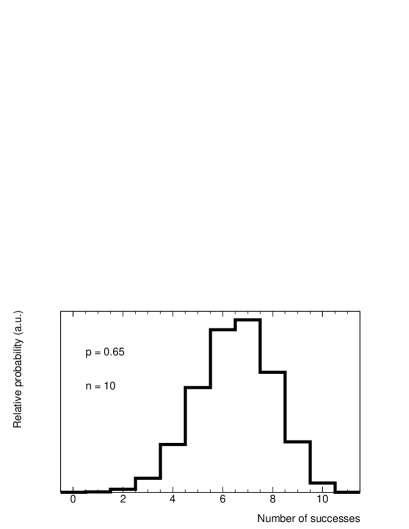
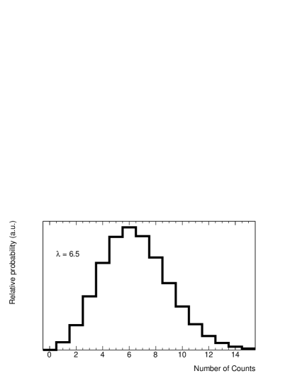
Figure 5: Examples of a Binomial (left) and a Poisson (right) distributions, with parameters $n=10$, $p=0.6$ and $\lambda=6.5$, respectively.

The Poisson distribution

In the $n\to\infty$, $p\to 0$ limit (with $\lambda=np$ finite and non-zero) for the Binomial distribution, the random variable $k$ follows the Poisson distribution $P(k;\lambda)$,

$$P_{\rm Poisson}\left(k;\lambda\right)\ =\ \frac{\lambda^{k}e^{-\lambda}}{k!}\ ,$$ (46)

for which $\lambda$ is the unique parameter. For Poisson, the mean value and variance are the same:

$$E\left[k\right]\ =\ V\left[k\right]\ =\ \lambda\ .$$ (47)

The Poisson distribution, sometimes called law of rare events (in view of the $p\to 0$ limit), is a useful model for describing event-counting rates. Examples of a Binomial and a Poisson distribution, for $n=10$, $p=0.6$ and for $\lambda=6.5$, respectively, are shown on Figure 5.

0.4.2 Common examples of real-valued distributions

The first two continuous random variables discussed in this paragraph are the uniform and the exponential distributions, illustrated in Figure 6.

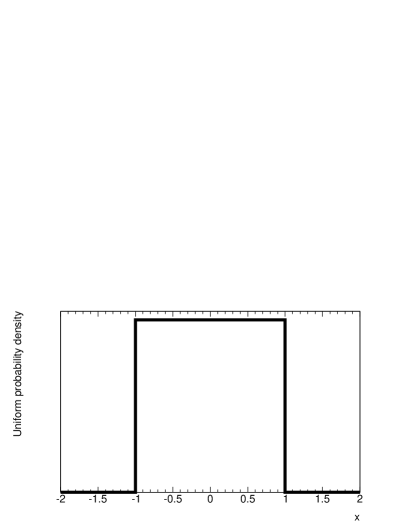
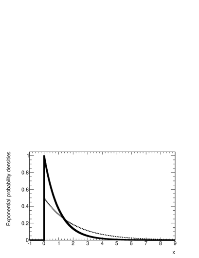
Figure 6: Examples of a uniform (left) and an exponentially-decreasing (right) distribution. For the uniform distribution, values used for the boundary parameters are $a=-1$, $b=1$; for the exponential, two values $\xi=1$ (solid line) and $\xi=2$ (dashed line) are used.

The uniform distribution

Consider a continuous random variable $x$, with a probability density $P(x;a,b)$ that is non-zero only inside a finite interval $\left[a,b\right]$:

$$P_{\rm uniform}\left(x;a,b\right)\ =\ \left\{\begin{array}[]{lcl}\frac{1}{b-a}&,&a\leq x\leq b\ ,\\ 0&,&{\rm otherwise}\ .\end{array}\right.$$ (50)

For this uniform distribution, the mean value and variance are

$$E\left[x\right] = \frac{a+b}{2}\ ,$$ (51)

$$V\left[x\right] = \frac{(b-a)^{2}}{12}\ .$$ (52)

While not being the most efficient one, a straightforward Monte-Carlo generation approach would be based on a uniform distribution in the $\left[0,p\right]$ range, and use randomly generated values of $x$ in the $\left[0,1\right]$ range as implementation of an accept-reject algorithm with success probability $p$.

The exponential distribution

Consider a continuous variable $x$, with a probability density $P(x;\xi)$ given by

$$P_{\rm exponential}\left(x;\xi\right)\ =\ \left\{\begin{array}[]{lcl}\frac{1}{\xi}e^{-x/\xi}&,&x\geq 0\ ,\\ 0&,&{\rm otherwise}\ ,\end{array}\right.$$ (55)

whose mean value and variance are

$$E\left[x\right] = \xi\ ,$$ (56)

$$V\left[x\right] = \xi^{2}\ .$$ (57)

A common application of this exponential distribution is the description of phenomena occuring independently at a constant rate, such as decay lengths and lifetimes. In view of the self-similar feature of the exponential function:

$$P(t-t_{0}|t>t_{0})\ =\ P(t)\ ,$$ (58)

the exponential distribution is sometimes said to be memoryless.

The Gaussian distribution

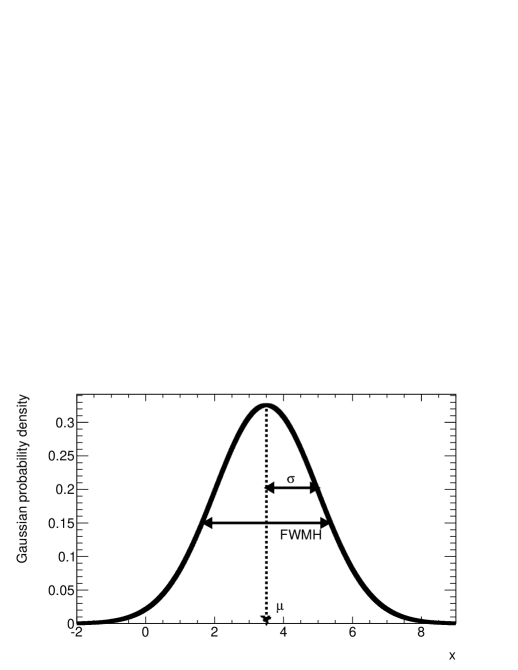
Figure 7: A Gaussian PDF, with parameter values $\mu=3.5$ and $\sigma=1.5$.

Now turn to the Normal (or Gaussian) distribution. Consider a random variable $x$, with probability density

$$P_{\rm Gauss}\left(x;\mu,\sigma\right)\ =\ \frac{1}{\sqrt{2\pi\sigma}}e^{-\frac{(x-\mu)^{2}}{2\sigma^{2}}}\ ,$$ (59)

and with mean value and variance given by

$$E\left[x\right]\ =\ \mu\ ,$$ (60)

$$V\left[x\right]\ =\ \sigma\ .$$ (61)

The PDF corresponding to the special $\mu=0$, $\sigma=1$ case is usually called “reduced normal”.

On purpose, the same symbols $\mu$ and $\sigma$ have been used both for the parameters of the Gaussian PDF and for the mean value and variance. This is an important feature: the Gaussian distribution is uniquely characterized by its first and second moments. For all Gaussians, the $\left[\mu-\sigma;\mu+\sigma\right]$ covers $68.3\%$ of PDF integral, and is customary called a “one-sigma interval”; similarly for the two-sigma interval and its $95.4\%$.

The dispersion of a peaked distribution is sometimes characterised in terms of its FWHM (full width at half-maximum); for Gaussian distributions, this quantity is uniquely related to its variance, as ${\rm FWHM}=2\sqrt{2\ln{2}}\simeq 2.35\sigma$; Figure 7 provides a graphical illustration of the Gaussian PDF and its parameters.

In terms of conceptual relevance and practical applications, the Gaussian certainly outnumbers all other common distributions; this feature is largely due to the central limit theorem, which asserts that Gaussian distributions are the limit of processes arising from multiple random fluctuations. Consider $n$ independent random variables $\vec{x}=\left\{x_{1},x_{2},\dotsc,x_{n}\right\}$, each with mean and variances $\mu_{i}$ and $\sigma_{i}^{2}$; the variable $S(\vec{x})$, built as the sum of reduced variables

$$S\ =\ \frac{1}{\sqrt{n}}\sum_{i=1}^{n}\frac{x_{i}-\mu_{i}}{\sigma_{i}}\ ,$$ (62)

can be shown to have a distribution that, in the large-$n$ limit, converges to a reduced normal distribution, as illustrated in Figure 8 for the sum of up to five uniform distributions. Not surprisingly, any measurement subject to multiple sources of fluctuations is likely to follow a distribution that can be approximated with a Gaussian distribution to a good approximation, regardless of the specific details of the processes at play.

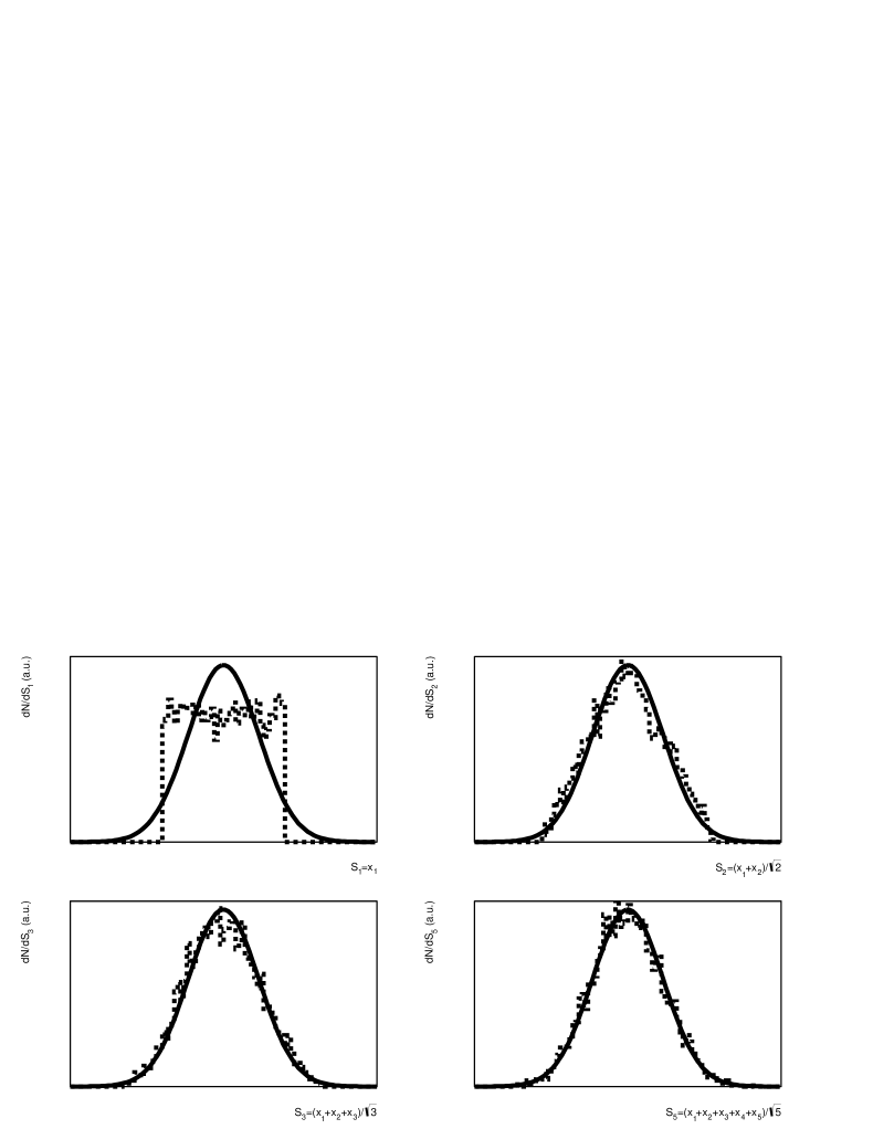
Figure 8: A graphical illustration of the central limit theorem. The top left plot compares the histogram (dashed curve) of a sample realization from a uniform variable $x_{1}$, with a normal PDF (solid line) of same mean and variance; similarly, the plots on the top right, bottom left and bottom right plot the corresponding histograms for the sums $S_{2}$, $S_{3}$ and $S_{5}$ of two, three and five reduced uniform variables $x_{1},\dotsc,x_{5}$, respectively. The sequence of variables follow distributions that quickly converge to a reduced Gaussian.

The Gaussian is also encountered as the limiting distribution for the Binomial and and Poisson ones, in the large $n$ and large $\lambda$ limits, respectively:

$$P_{\rm binomial}\left(k;n\to\infty,p\right) \rightarrow P_{\rm Gauss}\left(k;np,np(1-p)\right)\ ,$$ (63)

$$P_{\rm Poisson}\left(k;\lambda\to\infty\right) \rightarrow P_{\rm Gauss}\left(k;\lambda,\sqrt{\lambda}\right)\ .$$ (64)

Note that, when using a Gaussian as approximation, an appropriate continuity correction needs to be taken into account: the range of the Gaussian extends to negative values, while Binomial and Poisson are only defined in the positive range.

The $\chi^{2}$ distributions

Now the $\chi^{2}$ (or chi-squared) distributions are considered. The following PDF

$$P_{\rm\chi^{2}}\left(x;n\right)\ =\ \left\{\begin{array}[]{lcl}\frac{x^{n/2-1}e^{-x/2}}{2^{n/2-1}\Gamma\left(\frac{n}{2}\right)}&,&x\geq 0\ ,\\ 0&,&{\rm otherwise}\ ,\end{array}\right.$$ (67)

with a single parameter $n$, and where $\Gamma\left(n/2\right)$ denotes the Gamma function, has mean value and variance given by

$$E\left[x\right]\ =\ n\ ,$$

$$V\left[x\right]\ =\ 2n\ .$$ (68)

The shape of the $\chi^{2}$ distribution depends thus on $n$, as shown in Figure 9 where the $\chi^{2}$ PDF, for the first six integer values of the $n$ parameter, are shown.

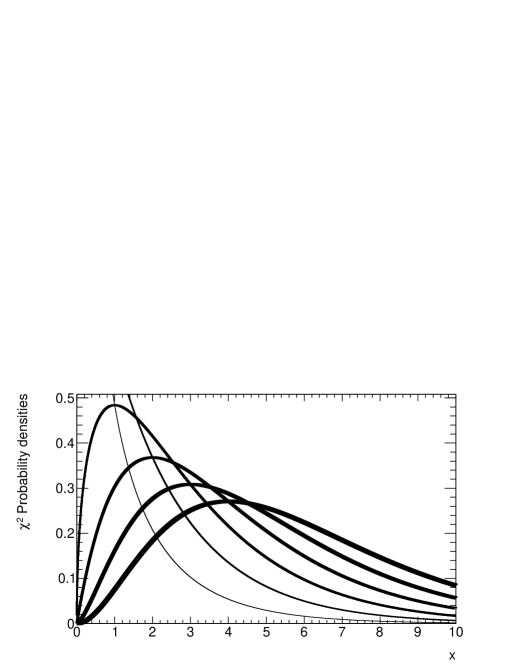
Figure 9: The first six $\chi^{2}$ probability density functions, for integer numbers of degrees of freedom $n$. The width of solid lines increases monotonically with $n$ in the $n=1,\dotsc,6$ range.

It can be shown that the $\chi^{2}$ distribution can be written as the sum of squares of $n$ normal-reduced variables $x_{i}$, each with mean $\mu_{i}$ and variance $\sigma_{i}^{2}$:

$$P_{\rm\chi^{2}}\left(x;n\right)\ =\ \sum_{i=1}^{n}\left(\frac{x_{i}-\mu_{i}}{\sigma_{i}}\right)^{2}\ .$$ (69)

In view of this important feature of the $\chi^{2}$ distribution, the quantity $n$ is called “number of degrees of freedom”; this name refers to the expected behaviour of a least-square fit, where $n_{d}$ data points are used to estimate $n_{p}$ parameters; the corresponding number of degrees of freedom is $n_{d}-n_{p}$. For a well-behaved fit, the $\chi^{2}$ value should follow a $\chi^{2}$ distribution. As discussed in 0.7.1, the comparison of an observed $\chi^{2}$ value with its expectation, is an example of goodness-of-fit test.

The Breit-Wigner and Voigtian distributions

The survey closes with the discussion of two physics-motivated PDFs. The first is the Breit-Wigner function, which is defined as

$$P_{\rm BW}\left(x;\Gamma,x_{0}\right)\ =\ \frac{1}{\pi}\frac{\Gamma/2}{\left(x-x_{0}\right)^{2}+\Gamma^{2}/4}\ ,$$ (70)

whose parameters are the most probable value $x_{0}$ (which specifies the peak of the distribution), and the FWHM $\Gamma$. The Breit-Wigner is also called Lorentzian by physicists, and in matematics it is often referred to as the Cauchy distribution. It has a peculiar feature, as a consequence of its long-range tails: the empirical average and empirical RMS are ill-defined (their variance increase with the size of the samples), and cannot be used as estimators of the Breit-Wigner parameters. The truncated mean and interquartile range, which are obtained by removing events in the low and high ends of the sample, are safer estimators of the Breit-Wigner parameters.

In the context of relativistic kinematics, the Breit-Wigner function provides a good description of a resonant process (for example the invariant mass of decay products from a resonant intermediate state); for a resonance, the parameters $x_{0}$ and $\Gamma$ are referred to as its mass and its natural width, respectively.

Finally, the Voigtian function is the convolution of a Breit-Wigner with a Gaussian,

$$P_{\rm Voigt}\left(x;x_{0},\Gamma,\sigma\right)\ =\ \int_{-\infty}^{+\infty}dx^{\prime}P_{\rm Gauss}\left(x^{\prime};0,\sigma\right)P_{\rm BW}\left(x-x^{\prime};x_{0},\Gamma\right)\ ,$$ (71)

and is thus a three-parameter distribution: mass $x_{0}$, natural width $\Gamma$ and resolution $\sigma$. While there is no straightforward analytical form for the Voigtian, efficient numerical implementations are available, i.e. the TMath::Voigt member function in the ROOT [7] data analysis framework, and the RooVoigtian class in the RooFit [8] toolkit for data modeling. For values of $\Gamma$ and $\sigma$ sufficiently similar, the FWHM of a Voigtian can be approximated as a combination of direct sums and sums in quadrature of the $\Gamma$ and $\sigma$ parameters. A simple, crude approximation yields :

$${\rm FWHM}_{\rm Voigt}\ \simeq\left[\left(\Gamma/2\right)\oplus\sigma\right]+\Gamma/2\ .$$ (72)

When the instrumental resolutions are sufficiently well described by a Gaussian, a Voigtian distribution is a good model for observed experimental distributions of a resonant process. Figure 10 represents an analytical Breit-Wigner PDF (evaluated using the $Z$ boson mass and width as parameters), and a dimuon invariant mass spectrum around the $Z$ boson mass peak, as measured by the ATLAS experiment using 8 TeV data [9]. The width of the observed peak is interpreted in terms of experimental resolution effects, as indicated by the good data/simulation agreement. Of course, the ATLAS dimuon mass resolution is more complicated than a simple Gaussian (as hinted by the slightly asymmetric shape of the distribution), therefore a simple Voigtian function would not have reached the level of accuracy provided by the complete simulation of the detector resolution.

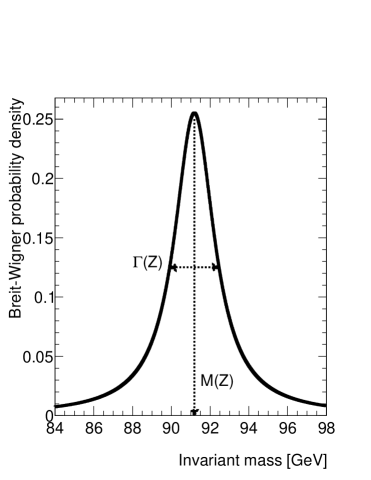
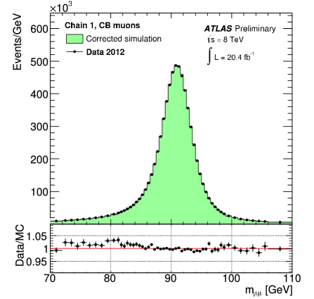
Figure 10: Left: the probability density function for a Breit-Wigner distribution, using the PDG [6] values for the $Z$ boson mass and width as parameters. Right: the invariant dimuon mass spectrum around the $Z$ boson mass peak; the figure is from an ATLAS measurement using 8 TeV data [9].

0.5 The maximum likelihood theorem and its applications

The discussion in Section 0.3.3 was aimed at describing a few intuitive examples of parameter estimation and their properties. Obviously, such case-by-case approaches are not general enough. The maximum likelihood estimation (MLE) is an important general method for parameter estimation, and is based on properties following the maximum likelihood (ML) theorem.

Consider a sample made of $N$ independent outcomes of random variables $\vec{x}$, arising from a $n$-parametric PDF $P\left(\vec{x};\theta_{1},\dotsc,\theta_{n}\right)$, and whose analytical dependence on variables and parameters is known, but for which the value(s) of at least one of its parameters $\theta$ is unknown. With the MLE, these values are extracted from an analytical expression, called the likelihood function, that has a functional dependence derived from the PDF, and is designed to maximise the probability of realizing the observed outcomes. The likelihood function ${\cal L}$ can be written as

$${\cal L}\left(\theta_{1},\dotsc,\theta_{n};\vec{x}\right)\ =\ \prod_{i=1}^{N}P\left(\vec{x}_{i};\theta_{1},\dotsc,\theta_{n}\right)\ .$$ (73)

This notation shows implictly the functional dependence of the likelihood on the parameters $\theta$, and on the $N$ realizations $\vec{x}$ of the sample. The ML theorem states that the $\hat{\theta_{1}},\dotsc,\theta_{n}=\hat{\theta}_{n}$ values that maximize ${\cal L}$,

$${\cal L}\left(\hat{\theta}_{1},\dotsc,\hat{\theta}_{n}\vec{x}\right)\ =\ \left.{\rm max}\right|_{\theta}\left\{{\cal L}\left(\theta_{1},\dotsc,\theta_{n}\right)\right\}\ .$$ (74)

are estimators of the unknown parameters $\theta$, with variances $\hat{\sigma}_{\theta}$ that are extracted from the covariance of ${\cal L}$ around its maximum.

In a few cases, the MLE can be solved analytically. A classical example is the estimation of the mean value and variance of an arbitrary sample, that can be analytically derived under the assumption that the underlying PDF is a Gaussian. Most often though, a numerical study of the likelihood around the $\theta$ parameter space is needed to localize the $\hat{\theta}$ point that minimizes $-\ln{{\cal L}}$ (the “negative log-likelihood”, or NLL); this procedure is called a ML fit.

0.5.1 Likelihood contours

Formally speaking, several conditions are required for the ML theorem to hold. For instance, ${\cal L}$ has to be at least twice derivable with respect to all its $\theta$ parameters; constraints on (asymptotical) unbiased behaviour and efficiency must be satisfied; and the shape of ${\cal L}$ around its maximum must be normally distributed. This last condition is particularly relevant, as it ensures the accurate extraction of errors. When it holds, the likelihood is said (in a slightly abusive manner) to have a “parabolic” shape (more in reference to $-\ln{L}$ than to the likelihood itself), and its expansion around $\hat{\theta}$ can be written as

$$f\left(\hat{\vec{\theta}},\vec{\theta},\mathbf{\Sigma}\right)\ =\ \frac{1}{\sqrt{2\pi}\left|\mathbf{\Sigma}\right|}\exp{\left\{-\frac{1}{2}\left(\hat{\vec{\theta}}_{i}-\vec{\theta}_{i}\right)\Sigma^{-1}_{ij}\left(\hat{\vec{\theta}}_{j}-\vec{\theta}_{j}\right)\right\}}\ .$$ (75)

In Eq. (75) the covariance matrix $\mathbf{\Sigma}$ has been introduced, and its elements are given by :

$$\mathbf{\Sigma}_{ij}^{-1}\ =\ -E\left[\frac{\partial\ln{\cal L}}{\partial\theta_{i}}\frac{\partial\ln{\cal L}}{\partial\theta_{j}}\right]\ .$$ (76)

When moving away from its maximum, the likelihood value decreases by amounts that depend on the covariance matrix elements:

$$-2\Delta\ln{\cal L}\ =\ -2\left[\ln{\cal L}(\vec{\theta})-\ln{\cal L}(\hat{\vec{\theta}})\right]\ =\ \sum_{i,j}\left(\theta_{i}-\hat{\theta}_{i}\right)\mathbf{\Sigma}_{ij}^{-1}\left(\theta_{i}-\hat{\theta}_{j}\right)\ .$$ (77)

This result, together with the result on error propagation in Eq. (37), indicates that the covariance matrix defines contour maps around the ML point, corresponding to confidence intervals. In the case of a single-parameter likelihood ${\cal L}(\theta)$, the interval contained in a $-2\Delta\ln{\cal L}<1$ contour around $\hat{\theta}$ defines a $68\%$ confidence interval, corresponding to a $-\sigma_{\theta}\leq\theta-\hat{\theta}\leq\sigma_{\theta}$ range around the ML point; in consequence the result of this MLE can be quoted as $\left(\hat{\theta}\pm\hat{\sigma}_{\theta}\right)$.

0.5.2 Selected topics on maximum likelihood

Samples composed of multiple species

In a typical scenario, the outcome of a random process may arise from multiple sources. To be specific, consider that events in the data sample are a composition of two “species”, called generically “signal” and “background” (the generalization to scenarios with more than two species is straighforward). Each species is supposed to be realized from its own probability densities, yielding similar (but not identical) signatures in terms of the random variables in the data sample; it is precisely these residual differences in PDF shapes that are used by the ML fit for a statistical separation of the sample into species. In the two-species example, the underlying total PDF is a combination of both signal and background PDFs, and the corresponding likelihood function is given by

$${\cal L}\left(\theta;\vec{x}\right)\ =\ \prod_{i=1}^{N}\left[f_{\rm sig}P_{\rm sig}(\vec{x};\theta)+(1-f_{\rm sig})P_{\rm bkg}(\vec{x};\theta)\right]\ ,$$ (78)

where $P_{\rm sig}$ and $P_{\rm bkg}$ are the PDFs for the signal and background species, respectively, and the signal fraction $f_{\rm sig}$ is the parameter quantifying the signal purity in the sample: $0\leq f_{\rm sig}\leq 1$. Note that, since both $P_{\rm sig}$ and $P_{\rm bkg}$ satisfy the PDF normalization condition from Eq. (9), the total PDF used in Eq. (78) is also normalized. It is worth mentioning that some of the parameters $\theta$ can be common to both signal and background PDFs, and others may be specific to a single species. Then, depending on the process and the study under consideration, the signal fraction can either have a known value, or belong to the set of unknown parameters $\theta$ to be estimated in a ML fit.

Extended ML fits

In event-counting experiments, the actual number of observed events of a given species is a quantity of interest; it is then convenient to treat the number of events as an additional parameter $\lambda$ of the likelihood function. In the case of a single species, this amounts to “extending” the likelihod,

$${\cal L}\left(\lambda,\theta;\vec{x}\right)\ =\ \frac{\lambda^{N}e^{-\lambda}}{N!}\prod_{i=1}^{N}P\left(\vec{x_{i}};\theta\right)\ .$$ (79)

where an additional multiplicative term, corresponding to the Poisson distribution (c.f. Section 0.4.1), has been introduced. (the $N!$ term in the denominator can be safely dropped; a global factor has no impact on the shape of the likelihood function nor on the ML fit results). It is straightforward to verify that the Poisson likelihod in Eq. (79) is maximal when $\hat{\lambda}=N$, as intended; now, if some of the PDFs also depend on $\lambda$, the value of $\hat{\lambda}$ that maximises ${\cal L}$ may differ from $N$. The generalization to more than one species is straightforward as well; for each species, a multiplicative Poisson term is included in the extended likelihood, and the PDFs of each species are weighted by their corresponding relative event fractions; in presence of two species, the extended version of the likelihood in Eq. 78 becomes:

$${\cal L}\left(N_{\rm sig},N_{\rm bkg}\theta;\vec{x}\right)\ =\ (N_{\rm sig}+N_{\rm bkg})^{N}e^{-(N_{\rm sig}+N_{\rm bkg})}\prod_{i=1}^{N}\left[N_{\rm sig}P_{\rm sig}(\vec{x};\theta)+N_{\rm bkg}P_{\rm bkg}(\vec{x};\theta)\right]\ .$$ (80)

“Non-parabolic” likelihoods, likelihoods with multiple maxima

As discussed in Section 0.5.1, the condition in Eq. (75) about the asymptotically normal distribution of the likelihood around its maximum is crucial to ensure a proper interpretation of $-2\Delta\ln{\cal L}$ contours in terms of confidence intervals. In this paragraph, two scenarios in which this condition can break down are discussed.

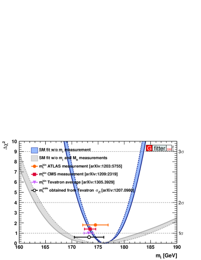
Figure 11: Left: two-dimensional likelihood contours in the $m_{w}-m_{t}$ plane, obtained from a global electroweak fit (EW) performed by the gFitter collaboration [10]. Center: the change in the EW likelihood as a function of $m_{t}$, expressed in terms of $\delta\chi^{2}=-2\Delta\ln{L}$. Both plots illustrate the non-parabolic shape of the EW likelihood.

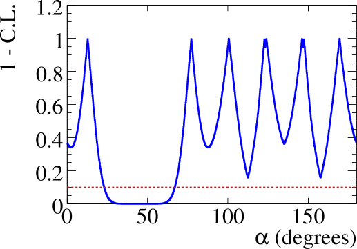
Figure 12: The change in likelihood, expressed in terms of a variant called “confidence level” CL, shown as a function of the CKM angle $\alpha$; the definition of CL is such that ${\rm CL}=0$ at the solutions of the ML fit. An eight-fold constraint on $\alpha$ is extracted from measurements in $B\rightarrow\pi\pi$ decays by the BABAR experiment [11]. The two pairs of solutions around $\sim 130^{\circ}$ are very close in values, and barely distinguishable in the figure.

A first scenario concerns a likelihood that is not totally symmetric around its maximum. Such a feature may occur, when studying low-statistics data samples, in view of the Binomial or Poissonian behaviour of event-counting related quantities (c.f. Figure 5). But it can also occur on larger-sized data samples, indicating that the model has a limited sensitivity to the parameter $\theta$ being estimated, or as a consequence of strong non-linear relations in the likelihood function. As illustration, examples of two- and one-dimensional likelihood contours, with clear non-parabolic shapes, are shown in Figure 11.

Also, the likelihood function may possess one or more local maxima, or even completely degenerate maxima. There are various possible sources for such degeneracies. For example in models with various species, if some PDF shapes are not different enough to provide a robust statistical discrimination among their corresponding species. For example, if swapping the PDFs for a pair of species yields a sufficiently good ML fit, a local maximum may emerge; on different sample realizations, the roles of local and global maxima may alternate among the correct and swapped combinations. The degeneracies could also arise as a reflexion of explicit, physical symmetries in the model: for example, time-dependent asymmetries in $B^{0}\rightarrow\pi^{+}\pi^{-}$ decays are sensitive to the CKM angle $\alpha$, but the physical observable is a function of $\cos{2(\alpha+\delta)}$, with an addtional phase $\delta$ at play; in consequence, the model brings up to eight indistinguishible solutions for the CKM angle $\alpha$, as illustrated in Figure 12.

In all such cases, the (possibly disjoint) $-2\Delta\ln{\cal L}<1$ interval(s) around the $\hat{\theta}$ central value(s) cannot be simply reported with a symmetric uncertainty $\hat{\sigma}_{\theta}$ only. In presence of a single, asymmetric solution, the measurement can be quoted with asymmetric errors, i.e. $\hat{\theta}^{+\sigma_{+}}_{-\sigma_{-}}$, or better yet, by providing the detailed shape of $-2\Delta\ln{\cal L}$ as a function of the estimated parameter $\theta$. For multiple solutions, more information needs to be provided: for example, amplitude analyses (“Dalitz-plot” analyses) produced by the B-factories BABAR and Belle, often reported the complete covariance matrices around each local solution (see e.g. [12, 13] as examples).

Estimating efficiencies with ML fits

Consider a process with two possible outcomes: “yes” and “no”. The intuitive estimator of the efficiency $\varepsilon$ is a simple ratio, expressed in terms of the number of outcomes $n_{\rm yes}$ and $n_{\rm no}$ of each kind:

$$\hat{\varepsilon}\ =\ \frac{n_{\rm yes}}{n_{\rm yes}+n_{\rm no}}\ ,$$ (81)

for which the variance is given by

$$V\left[\hat{\varepsilon}\right]\ =\ \frac{\hat{\varepsilon}(1-\hat{\varepsilon})}{n}\ ,$$ (82)

where $n=n_{\rm yes}+n_{\rm no}$ is the total number of outcomes realized. This estimator $\hat{\varepsilon}$ clearly breaks down for low $n$, and in the very low or very high efficiency regimes. The MLE technique offers a robust approach to estimate efficiencies: consider a PDF $P(x;\theta)$ to model the sample, and include in it an additional discrete, bivariate random variable $c=\left\{{\rm yes},{\rm no}\right\}$, so that the PDF becomes

$$P\left(x,c;\theta\right)\ =\ \delta(c-{\rm yes})\varepsilon(x,\theta)+\delta(c-{\rm no})\left[1-\varepsilon(x,\theta)\right]\ .$$ (83)

In this way, the efficiency is no longer a single number, but a function of $x$ (plus some parameters $\theta$ that may be needed to characterize its shape). With this function, the efficiency can be extracted in different $x$ domains, as illustated in Figure 13, or can be used to produce a multidimensional efficiency map.

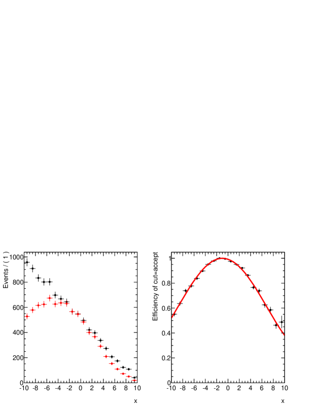
Figure 13: Left: the frequency of events in a sample, as a function of a variable $x$. The sample contains two categories of events: “accepted” and “rejected”. The red dots indicate the bins of the histogram for those “accepted” only, and the black dots for the two categories cumulated. Right: the efficiency as a parametric function of $x$, with parameter values extracted from a ML fit to the data sample. Figure extracted from the RooFit user’s guide [8].

0.5.3 Systematic uncertainties

As discussed in Section 0.5.1, in MLE the covariance of ${\cal L}$ is the estimator of statistical uncertainties. Other potential sources of (systematical) uncertainties are usually at play, and need to be quantified. For this discussion, a slight change in the notation with respect to Eq.(73) is useful; in this notation, the likelihood function is now written as

$${\cal L}\left(\mu_{1},\dotsc,\mu_{p}\ ,\ \theta_{1},\dotsc,\theta_{k};\vec{x}\right)\ ,$$ (84)

where the parameters are explicitly partitioned into a set $\mu_{1},\dotsc,\mu_{p}$, called parameters of interest (POI), that correspond to the actual quantities that are to be estimated; and a set $\theta_{1},\dotsc,\theta_{k}$, called nuisance parameters (NP), that represent potential sources of systematic biases: if inaccurate or wrong values are assigned to some NPs, the shapes of the PDFs can be distorted, the estimators of POIs can become biased. The systematic uncertainties due to NPs are usually classified in two categories.

The first category refers to “Type-I” errors, for which the sample (or other control data samples) can (in principle) provide information on the NPs under consideration, and are (in principle) supposed to decrease with sample size. The second category refers to “Type-II” errors, which arise from incorrect assumptions in the model (i.e. a choice of inadequate functional dependences in the PDFs), or uncontrolled features in data that can not be described by the model, like the presence of unaccounted species. Clearly, for Type-II errors the task of assigning systematic uncertainties to them may not be well-defined, and may spoil the statistical interpretation of errors in termos of confidence levels.

The profile-likelihod method

To deal with Type-I nuisance parameters, a popular approach is to use the so-called profile-likelihood method. This approach consists of assigning a specific likelihood to the nuisance parameters, so that the original likelihood is modified to have two different components:

$${\cal L}\left(\mu,\theta\right)\ =\ {\cal L}_{\mu}\left(\mu,\theta\right){\cal L}_{\theta}\left(\theta\right)\ .$$ (85)

Then, for a fixed value of $\mu$, the likelihood is maximized with respect to the nuisance $\theta$; the sequencial outcome of this procedure, called profile likelihood, is a function that depends only on $\mu$: it is then said that the nuisance parameter has been profiled out of the likelihood.

As an example, consider the measurement of the cross-section of a generic process, $\sigma\left({\rm initial}\to{\rm final}\right)$. If only a fraction of the processes is actually detected, the efficiency $\varepsilon$ of reconstructing the final state is needed to convert the observed event rate $\hat{N}_{\rm event}$ into a measurement $\hat{\sigma}$. This efficiency is clearly a nuisance: a wrong value of $\varepsilon$ directly affects the value of $\hat{\sigma}$, regardless of how accurately $\hat{N}_{\rm event}$ may have been measured. By estimating $\hat{\varepsilon}$ on a quality control sample (for example, high-statistics simulation, or a high-purity control data sample), the impact of this nuisance can be attenuated. For example, an elegant analysis would produce a simultaneous fit to the data and control samples, so that the values and uncertainties of NPs are estimated in the ML fit, and are correctly propagated to the values and variances of the POIs.

As another example, consider the search for a resonance (“a bump”) over a uniform background. If the signal fraction is very small, the width $\Gamma$ of the bump cannot be directly estimated on data, and the value used in the signal PDF has to be inferred from external sources. This width is clearly a nuisance: using an overestimated value would translate into an underestimation of the signal-to-background ratio, and thus an increase in the variance of the signal POIs, and possibly biases in their central values as well, i.e. the signal rate would tend to be overestimated. Similar considerations can be applied in case of underestimation of the width. If an estimation $\hat{\Gamma}\pm\hat{\sigma}_{\Gamma}$ of the width is available, this information can be implemented as in Eq. (85), by using a Gaussian PDF, with mean value $\hat{\Gamma}$ and width $\hat{\Gamma}$, in the ${\cal L}_{\Gamma}$ component of the likelihood. This term acts as a penalty in the ML fit, and thus constraints the impact of the nuisance $\Gamma$ on the POIs.

0.6 Multivariate techniques

Often, there are large regions in sample space where backgrounds are overwhelming, and/or signals are absent. By restricting the data sample to “signal-enriched” subsets of the complete space, the loss of information may be minimal, and other advantages may compensate the potential losses: in particular for multi-dimensional samples, it can be difficult to characterize the shapes in regions away from the core, where the event densities are low; also reducing the sample size can relieve speed and memory consumption in numerical computations.

The simplest method of sample reduction is by requiring a set of variables to be restricted into finite intervals. In practice, such “cut-based” selections appear at many levels in the definition of sample space: thresholds on online trigger decisions, filters at various levels of data acquisition, removal of data failing quality criteria… But at more advanced stages of a data analysis, such “accept-reject” sharp selections may have to be replaced by more sophisticated procedures, generically called multivariate techniques.

A multi-dimensional ML fit is an example of a multivariate technique. For a MLE to be considered, a key requirement is to ensure a robust knowledge of all PDFs over the space of random variables.

Consider a set of $n$ random variables $\vec{x}=\left\{x_{1},x_{2}\dotsc,x_{n}\right\}$. If all variables are shown to be uncorrelated, their $n$-dimensional PDF is completely determined by the product of their $n$ one-dimensional PDFs; now, if variables are correlated, but their correlation patterns are completely linear, one can instead use variables $\vec{y}$, linear combinations of $\vec{x}$ obtained by diagonalizing the inverse covariance. For some non-linear correlation patterns, it may be possible to find analytical descriptions; for instance, the (mildly) non-linear correlation pattern represented in Figure 2, was produced with the RooFit package, by applying the Conditional option in RooProdPdf to build a product of PDFs. In practice, this elegant approach cannot be easily extended to more than two dimensions, and is not guaranteed to reproduce complex, non-linear patterns. In such scenarios, the approach of dimensional reduction can potentially bring more effective results.

A typical scenario for dimensional reduction is when several variables carry common information (and thus exhibit strong correlations), together with some diluted (but relevant) pieces of independent information. An example is the characterization of showers in calorimeters; for detectors with good transverse and/or longitudinal segmentation, the signals deposited in nearby calorimetric channels can be used to reconstruct details from the shower development; for example, a function that combines informations from longitudinal and transverse shower shapes, can be used to discriminate among electromagnetic and hadronic showers.

The simplest algorithm for dimensional reduction is the Fisher discriminant: it is a linear function of variables, with coefficients adjusted to match an optimal criterion, called separation among two species, which is is the ratio of the variance between the species to the variance within the species, and can be expressed in a close, simple analytical form.

In presence of more complex, non-linear correlation patterns, a large variety of techniques and tools are available. The TMVA [14] package is a popular implementation of dimensional-reduction algorithms; other than linear and likelihood-based discriminants, it provides easy training and testing methods for artificial neural networks and (boosted) decision trees, which are among those most often encountered in HEP analyses. As a general rule, a multivariate analyzer uses a collection of variables, realized on two different samples (corresponding to “signal” and “background” species), to perform a method-dependent training, guided by some optimization criteria; then performances of the trained analyzer are evaluated on independent realizations of the species (this distinction between the training and testing stages is crucial to avoid “over-training” effects). Figure 14 shows a graphical representation of a figure-of-merit comparison of various analyzers implemented in TMVA.

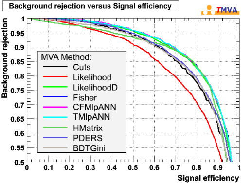
Figure 14: A figure-of-merit comparison between various different multivariate analyzer methods using the TMVA package. The training was performed on two simulated samples (“signal” and “background”), each consisting of four linearly correlated Gaussian-distributed variables. The various lines indicate the trade-off between signal efficiency and background rejection. The figure is taken from [14].

0.7 Statistical hypothesis testing

Sections 0.3 and 0.5 mainly discussed procedures for extracting numerical information from data samples; that is, to perform measurements and report them in terms of values and uncertanties. The next step in data analysis is to extract qualitative information from data: this is the domain of statistical hypothesis testing. The analytical tool to assess the agreement of an hypothesis with observations is called a test statistic, (or a statistic in short); the outcome of a test is given in terms of a $p$-value, or probability of a “worse” agreement than the one actually observed.

0.7.1 The $\chi^{2}$ test

For a set of $n$ independent measurements $x_{i}$, their deviation with respect to predicted values $\mu_{i}$, expressed in units of their variances $\sigma_{i}$ is called the $\chi^{2}$ test, and is defined as

$$\chi^{2}\ =\ \sum_{\rm i=1}^{n}\left(\frac{x_{i}-\mu_{i}}{\sigma_{i}}\right)^{2}\ .$$ (86)

An ensemble of $\chi^{2}$ tests is a random variable that, as mentioned in Section 0.4.2, follows the $P_{\chi^{2}}$ distribution (c.f. Eq. 67) for $n$ degrees of freedom. Its expectation value is $n$ and its variance $2n$; therefore one does expect the $\chi^{2}$ value observed in a given test not to deviate much from the number of degrees of freedom, and so this value can be used to probe the agreement of prediction and observation. More precisely, one expects $68\%$ of tests to be contained within a $n\pm\sqrt{2n}$ interval, and the $p$-value, or probability of having a test with values larger than a given $\chi^{2}$ value is

$$p\ =\ \int_{\chi^{2}}^{+\infty}dq\ P_{\chi^{2}}\left(q;n\right)\ .$$ (87)

Roughly speaking, one would tend to be suspicious of small observed $p$-values, as they may indicate a trouble, either with the prediction or the data quality. The interpretation of the observed $p$-value (i.e. to decide whether it is too small or large enough) is an important topic, and is discussed below in a more general approach.

0.7.2 General properties of hypothesis testing

Consider two mutually excluding hypotheses $H_{0}$ and $H_{1}$, that may describe some data sample; the hypothesis testing procedure states how robust is $H_{0}$ to describe the observed data, and how incompatible is $H_{1}$ with the observed data. The hypothesis $H_{0}$ being tested is called the “null” hypothesis, while $H_{1}$ is the “alternative” hypothesis,

Note that in the context of the search for a (yet unknown) signal, the null $H_{0}$ corresponds to a “background-only” scenario, and the alternative $H_{1}$ to “signal-plus-background”; while in the context of excluding a (supposedly inexistent) signal, the roles of the null and alternative hypotheses are reversed: the null $H_{0}$ is “signal-plus-background” and the alternative $H_{1}$ is “background-only”.

The sequence of a generic test, aiming at accepting (or rejecting) the null hypothesis $H_{0}$ by confronting it to a data sample, can be sketched as follows:

• build a test statistic $q$, that is, a function that reduces a data sample to a single numerical value;

• define a confidence interval $W\ \rightarrow\ \left[q_{\rm lo}:q_{\rm hi}\right]$;

• measure $\hat{q}$;

• if $\hat{q}$ is contained in $W$, declare the null hypothesis accepted; otherwise, declare it rejected.

To characterize the outcome of this sequence, two criteria are defined: a “Type-I error” is incurred in, if $H_{0}$ is rejected despite being true; while a “Type-II error” is incurred in, if $H_{0}$ is accepted despite being false (and thus $H_{1}$ being true). The rates of Type-I and Type-II errors are called $\alpha$ and $\beta$ respectively, and are determined by integrating the $H_{0}$ and $H_{1}$ probability densities over the confidence interal $W$,

$$1-\alpha = \int_{W}dq{\cal P}\left(q|H_{0}\right)\ ,$$

$$\beta = \int_{W}dq{\cal P}\left(q|H_{1}\right)\ .$$ (88)

The rate $\alpha$ is also called “size of the test” (or size, in short), as fixing $\alpha$ determines the size of the confidence interval $W$. Similarly, $1-\beta$ is also called “power”. Together, size and power characterize the performance of a test statistic; the Neyman-Pearson lemma states that the optimal statistic is the likelihood ratio $q_{\lambda}$,

$$q_{\lambda}\left({\rm data}\right)\ =\ \frac{{\cal L}\left({\rm data}|H_{0}\right)}{{\cal L}\left({\rm data}|H_{1}\right)}\ .$$ (89)

The significance of the test is given by the $p$-value,

$$p\ =\ \int_{\hat{q}}^{+\infty}dq{\cal P}\left(q|H_{0}\right)\ .$$ (90)

which is often quoted in terms of “sigmas”,

$$p\ =\ \int_{n\sigma}^{+\infty}dz\frac{1}{\sqrt{2\pi}}e^{-z^{2}/2}\ =\ 1-\frac{1}{2}{\rm erf}\left(\frac{n}{\sqrt{2}}\right)\ ,$$ (91)

so that for example a $p<0.0228$ outcome can be reported as a “two-sigma” effect. Alternatively, it is common practice to quote the complement of the $p$-value as a confidence level (C.L.).

The definition of a $p$-value as in Eq. (90) (or similarly in Eq. (87) for the example for a $\chi^{2}$ test) is clear and unambiguous. But interpretation of $p$-values is partly subjective: the convenience of a numerical “threshold of tolerance” may depend on the kind of hypothesis being tested, or on common practice. In HEP usage, three different traditional benchmarks are conventionally employed:

• in exclusion logic, a $95\%$ C.L. threshold on a signal-plus-background test to claim exclusion;

• in discovery logic, a three-sigma threshold ($p<1.35\times 10^{-3}$) on a background-only test to claim “evidence”;

• and a five-sigma threshold ($p<2.87\times 10^{-7}$) on the background-only test is required to reach the “observation” benchmark.

0.7.3 From LEP to LHC: statistics in particle physics

In experimental HEP, there is a tradition of reaching consensual agreement on the choices of test statistics. The goal is to ensure that, in the combination of results from different samples and instruments, the detector-related components (specific to each experiment) factor out from the physics-related observables (which are supposed to be universal). For example in the context of searches for the Standard Model (SM) Higgs boson, the four LEP experiments agreed on analyzing their data using the following template for their likelihoods:

$${\cal L}\left(H_{1}\right) = \prod_{a=1}^{N_{\rm ch}}{\cal P}_{\rm Poisson}\left(n_{a},s_{a}+b_{a}\right)\prod_{j=1}^{n_{a}}\frac{s_{a}{\cal S}_{a}(\vec{x_{j}})+b_{a}{\cal B}_{a}(\vec{x_{j}})}{s_{a}+b_{a}}\ ,$$

$${\cal L}\left(H_{0}\right) = \prod_{a=1}^{N_{\rm ch}}{\cal P}_{\rm Poisson}\left(n_{a},b_{a}\right)\prod_{j=1}^{n_{a}}{\cal B}_{a}(\vec{x_{j}})\ .$$ (92)

where $N_{\rm ch}$ is the number of Higgs decay channels studied, $n_{a}$ is the observed number of event candidates in channel $a$, ${\cal S}_{a}$ and $s_{a}$ (${\cal B}_{a}$ and $b_{a}$) are the PDF and event yield for the signal (background) species in that channel. Also, the test statistic $\lambda$, derived from a likelihood ratio, is

$$\lambda\ =\ -2\ln{Q}\ ,\ {\rm with}\ Q = \frac{{\cal L}\left(H_{1}\right)}{{\cal L}\left(H_{0}\right)}\ ;$$ (93)

so that roughly speaking, positive values of $\lambda$ favour a “background-like” scenario, and negative ones are more in tune with a “signal-plus-background” scenario; values close to zero indicate poor sensitivity to distinguish among the two scenarios. The values use to test these two hypotheses are:

• under the background-only hypothesis, ${\rm CL}(b)$ is the probability of having a $-2\ln{Q}$ value larger than the observed one;

• under the signal+plus+background hypothesis, ${\rm CL}(s+b)$ is the probability of having a $-2\ln{Q}$ value larger than the observed one.

Figure 15 shows, for three different Higgs mass hypotheses, the $-2\ln{Q}$ values from the combination of the four LEP experiments in their searches for the SM Higgs boson, overlaid with the expected ${\rm CL}(s+b)$ and $1-{\rm CL}(b)$ distributions. Figure 16 shows the evolution of $-2\ln{Q}$ values as a function of the hypothetized Higgs boson mass; (as stated in the captions, the color conventions in the one- and two-dimensional plots are different) note that for masses below $\sim 115$ GeV, a positive value of the $-2\ln{Q}$ test statistic would have provided evidence for a signal; and sensitivity is quickly lost above that mass.

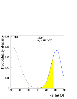
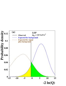
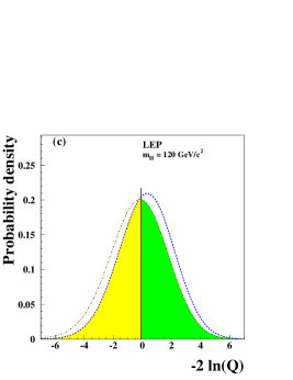
Figure 15: Combined results from the search for a SM Higgs boson, performed by the four LEP experiments. From left to right, the $m_{H}=110,115,120$ GeV hypotheses for the Higgs mass are used. The dashed blue and dashed red lines correspond to the PDFs for the background-only and signal-plus-background hypotheses, respectively. The observed values of the test statistic $-2\ln{Q}$ are marked by black vertical lines. The yellow areas indicate the $1-{\rm CL}(b)$ values for the background-only hypothesis, and the green areas the ${\rm CL}(s+b)$ value for signal-plus-background. The three figures are taken from [17].

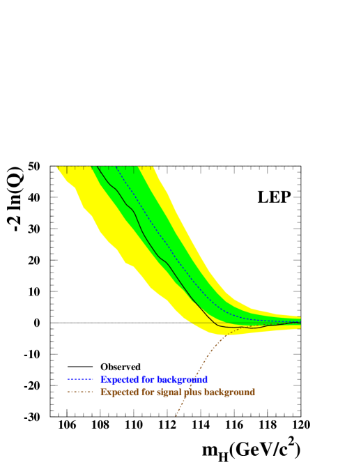
Figure 16: The test statistic $-2\ln{Q}$ as a function of the Higgs boson mass $m_{H}$, obtained by combining the data of the four LEP experiments. The dashed line is the mean value of the background-only distribution at each mass $m_{H}$, and the green and yellow areas represent $68\%$ and $95\%$ contours for the background-only distribution at each mass $m_{H}$. The black line follows the $-2\ln{Q}$ value observed in data as a function of $m_{H}$. Figure taken from [17].

The modified ${\rm CL}(s)$ hypothesis testing

The choice of ${\rm CL}(s+b)$ to test the signal-plus-background hypothesis, while suitably defined as a $p$-value. may drag some subjective concern: in case of a fortuitous simultaneous downward fluctuation in both signal and background, the standard $95\%$ benchmark may lead to an exclusion of the signal, even if the sensitivity is poor.

A modification of the exclusion benchmark called ${\rm CL}(s)$, has been introduced in this spirit[18], and is defined as

$${\rm CL}(s)\ =\ \frac{{\rm CL}(s+b)}{1-{\rm CL}(b)}\ .$$ (94)

This test, while not corresponding to a $p$-value (a ratio of probabilities is not a probability), has the desired property of protecting against downwards fluctuations of the background, and is commonly used in exclusion results, including the searches for the SM Higgs boson from the Tevatron and LHC experiments.

Profiled likelihood ratios

Following the recommendations from the LHC Higgs Combination Group [19], the ATLAS and CMS experiments have agreed on using a common test statistic, called profiled likelihood ratio and defined as

$$\tilde{q}_{\mu}\left(\mu\right)\ =\ -2\ln{\frac{{\cal L}\left(\mu,\hat{\hat{\theta}}\right)}{{\cal L}\left(\hat{\mu},\hat{\theta}\right)}}\ ,\ {\rm with}\ 0\leq\hat{\mu}\leq\mu\ ,$$ (95)

where the PIO $\mu=\sigma/\sigma_{\rm SM}$ is the “signal strength modifier”, or Higgs signal rate expressed in units of the SM predicted rate, $\hat{\hat{\theta}}$ are the fitted values of the NPs at fixed values of the signal strength, and $\hat{\mu}$ and $\hat{\theta}$ are the fitted values when both $\mu$ and NPs are all free to vary in the ML fit . The lower constraint on $0\leq\hat{\mu}\leq\mu$ ensures that the signal rate is positive, and the upper constraint imposes that an upward fluctuation would not disfavor the SM signal hypothesis.

For an observed statistic value $\hat{\tilde{q}}_{\mu}$, the $p$-values for testing the signal-plus-background and background-only hypotheses, $p(s+b)$ and $p(b)$, are

$$p(s+b) = \int_{\hat{\tilde{q}}_{\mu}}^{\infty}dqP\left(q;\mu=\hat{\mu},\hat{\theta}\right)\ ,$$ (96)

$$1-p(b) = \int_{\hat{\tilde{q}}_{\mu}}^{\infty}dqP\left(q;\mu=0,\hat{\hat{\theta}}\right)\ .$$ (97)

and the results on searches are reported both in terms of the exclusion significance using the ${\rm CL}(s)$ observed and expected values, and the observation significance expressed in terms of the “local”  $p(b)$ expected and observed values.

To conclude the discussion on hypothesis testing, there is certainly no better illustration than Figure 17, taken from the results announced by the ATLAS and CMS experiments on July 4th, 2012: in the context of the search for the SM Higgs boson, both collaborations established the observation of a new particle with a mass around 125 GeV.

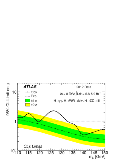
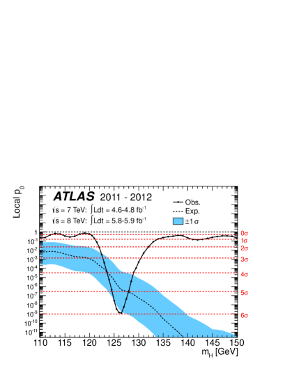
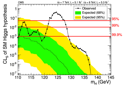
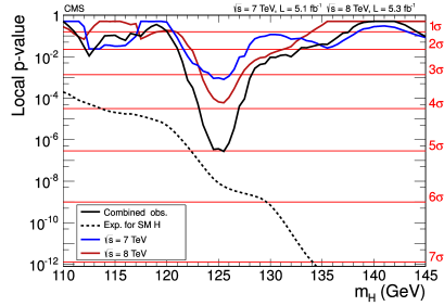
Figure 17: The expected distributions and observed values for the exclusion (left) and the observation significances (right) in searches for the SM Higgs boson presented by the ATLAS[21] (top) and CMS[22] (bottom) collaborations on July 4th, 2012. Both experiments find a significant excess around 125 GeV.

0.8 Conclusions

These lectures aimed at providing a pedagogical overview of probability and statistics. The choice of topics was driven by practical considerations, based on the tools and concepts actually encountered in experimental high-energy physics. A bias in the choices, induced by the author’s perspective and personal experience is not to be excluded. The discussion was completed with examples from recent results, mostly (although not exclusively) stemming from the $B$-factories and the LHC experiments.

0.9 Acknowledgements

I would like to express my gratitude to all who helped make the AEPSHEP 2012 school a success: the organizers, the students, my fellow lecturers and discussion leaders. The highly stimulating atmosphere brought fruitful interactions during lectures, discussion sessions and conviviality activities.

References

- [1] A. Stuart, J.K. Ord, and S. Arnold, Kendall’s Advanced Theory of Statistics, Vol. 2A: Classical Inference and the Linear Model 6th Ed., Oxford Univ. Press (1999), and earlier editions by Kendall and Stuart.
- [2] R.J. Barlow, Statistics: A Guide to the Use of Statistical Methods in the Physical Sciences, Wiley, 1989.
- [3] G.D. Cowan, Statistical Data Analysis, Oxford University Press, 1998.
- [4] F. James, Statistical Methods in Experimental Physics, 2nd ed., World Scientific, 2006.
- [5] L. Lyons, Statistics for Nuclear and Particle Physicists, Cambridge University Press, 1986.
- [6] J. Beringer et al. [Particle Data Group Collaboration], Phys. Rev. D 86, 010001 (2012).
- [7] R. Brun and F. Rademakers, Nucl. Instrum. Meth. A 389, 81 (1997).
- [8] W. Verkerke and D. P. Kirkby, eConf C 0303241, MOLT007 (2003).
- [9] The ATLAS collaboration, ATLAS-CONF-2013-088.
- [10] M. Baak, M. Goebel, J. Haller, A. Hoecker, D. Kennedy, R. Kogler, K. Moenig and M. Schott et al., Eur. Phys. J. C 72, 2205 (2012).
- [11] J. P. Lees [BaBar Collaboration], Phys. Rev. D 87, no. 5, 052009 (2013).
- [12] B. Aubert et al. [BaBar Collaboration], Phys. Rev. D 80 (2009) 112001.
- [13] J. Dalseno et al. [Belle Collaboration], Phys. Rev. D 79, 072004 (2009).
- [14] A. Hoecker, P. Speckmayer, J. Stelzer, J. Therhaag, E. von Toerne, and H. Voss, “TMVA: Toolkit for Multivariate Data Analysis,” PoS A CAT 040 (2007).
- [15] K. Cranmer et al. [ROOT Collaboration], “HistFactory: A tool for creating statistical models for use with RooFit and RooStats,” CERN-OPEN-2012-016.
- [16] L. Moneta, K. Belasco, K. S. Cranmer, S. Kreiss, A. Lazzaro, D. Piparo, G. Schott and W. Verkerke et al., The RooStats Project,” PoS ACAT 2010, 057 (2010).
- [17] R. Barate et al. [LEP Working Group for Higgs boson searches and ALEPH and DELPHI and L3 and OPAL Collaborations], Phys. Lett. B 565, 61 (2003).
- [18] A. L. Read, J. Phys. G 28, 2693 (2002).
- [19] [ATLAS and CMS Collaborations], “Procedure for the LHC Higgs boson search combination in summer 2011,” ATL-PHYS-PUB-2011-011, CMS-NOTE-2011-005.
- [20] G. Cowan, K. Cranmer, E. Gross and O. Vitells, Eur. Phys. J. C 71, 1554 (2011)
- [21] G. Aad et al. [ATLAS Collaboration], Phys. Lett. B 716, 1 (2012).
- [22] S. Chatrchyan et al. [CMS Collaboration], Phys. Lett. B 716, 30 (2012).