Quantum impurity in a Tomonaga-Luttinger liquid: continuous-time quantum Monte Carlo approach

K. Hattori1,2 hattori@issp.u-tokyo.ac.jp    A. Rosch1 1Institut für Theoretische Physik, Universität zu Köln, Zülpicher Str., 77, D-50937 Köln, Germany
2Institute for Solid State Physics, University of Tokyo, 5-1-5, Kashiwanoha, Kashiwa, Chiba 277-8581, Japan
Abstract

We develop a continuous-time quantum Monte Carlo (CTQMC) method for quantum impurities coupled to interacting quantum wires described by a Tomonaga-Luttinger liquid. The method is negative-sign free for any values of the Tomonaga-Luttinger parameter, which is rigorously proved, and thus, efficient low-temperature calculations are possible. Duality between electrons and bosons in one dimensional systems allows us to construct a simple formula for the CTQMC algorithm in these systems. We show that the CTQMC for Tomonaga-Luttinger liquids can be implemented with only minor modifications of previous CTQMC codes developed for impurities coupled to non-interacting fermions. We apply this method to the Kane-Fisher model of a potential scatterer in a spin-less quantum wire and to a single spin coupled with the edge state of a two-dimensional topological insulator assuming an anisotropic XXZ coupling. Various dynamical response functions such as the electron Green’s function and spin-spin correlation functions are calculated numerically and their scaling properties are discussed.

pacs:
68.65.La, 71.10.Pm, 75.40.Mg

I Introduction

Electronic correlations play fundamental roles in determining low-energy phenomena in one-dimensional electron systems TLL ; Giam . Bosonization is a powerful technique to treat such correlations exactly. In the presence of impurities, however, it is well known that impurities in one-dimensional systems drastically influence transport properties of the systems. Such an example has been found in a classical model by Kane and Fisher in their pioneering work about a backward scattering potential problem in a spinless quantum wire KF . There, for the case of repulsive interaction [Tomonaga-Luttinger (TL) parameter g<1𝑔1g<1], the conductance G𝐺G vanishes at zero temperature (T=0𝑇0T=0) and the potential barrier becomes infinitely strong and cut the wire into two parts, while for attractive cases with g>1𝑔1g>1, the potential becomes zero in the low-energy limit and there remains a finite value of the conductance at T=0𝑇0T=0.

For acquiring knowledge about thermodynamic, transport, and dynamical properties of such systems, bosonization combined with perturbative renormalization group methods KF ; Delft ; Furusaki , Bethe ansatz Bethe , and functional renormalization group fRG have been intensively used so far. To obtain numerically exact results for bosonized impurity problems, path integral Monte Carlo approaches have been employed PIMC1 ; PIMC2 ; PIMC3 . A bosonic numerical renormalization group method nrg is also a powerful technique to investigate their low-energy properties. While they are very useful approaches, there is still need for even more powerful numerical approaches that allow to compute wide range of temperature properties and dynamical correlation functions even for more complex models in an exact way.

To this end, in this paper, we will develop a continuous-time quantum Monte Carlo (CTQMC) method Rubtsov ; Werner ; Otsuki ; Gull in the Tomonaga-Luttinger liquid (TLL) in one-dimensional systems coupled to an impurity. The CTQMC previously has been developed to describe quantum impurities coupled to non-interacting environments. It has mainly been used for fermionic systems and extensively used in the frame work of the dynamical mean field theory DMFT as an exact numerical solver for the effective-impurity problem in it. Recent development Anders ; Otsuki-b of the algorithm also enables us to treat bosonic systems and mixture of bosons and fermions. The advantage of the CTQMC is that this allows us to calculate various quantities at low temperatures in efficient ways and for some simple models there is no negative sign problem Werner ; Otsuki .

Our algorithm of CTQMC for TLL has advantages in the following points. (i) Bosonization allows us to treat correlation arising from strong interactions in the environment exactly. (ii) There is no negative sign problem for any parameters, which is, indeed, proved analytically. This enables us to carry out low-temperature analysis with high precision. (iii) There are close relations to the fermionic version of CTQMC, although the whole algorithm is written in the bosonization language. This enables ones to implement the CTQMC for the TLL easily from their fermionic CTQMC code. (iv) The method can be applicable to not only potential scattering problems but also to Kondo-type problems Wu ; Mac0 ; Mac without a negative sign problem. (v) The electron Green’s functions, the boson-boson correlations, conductance, the spin-spin correlation functions, and various local correlators are calculable. (vi) Compared with lattice QMCs, our formalism is free from finite size effects at low temperatures and phase spaces for the random walk is expected to be much smaller, and, thus, the computational cost is much lower.

This paper is organized as follows. In Sec. II, we will explain the models used in this paper. Section III will be devoted to illustrate our algorithm of the CTQMC for TLL. The method will be applied to the Kane-Fisher model KF in Sec. IV.1 and the XXZ Kondo problem Wu ; Mac0 ; Mac in Sec. IV.2. We will discuss possible extension in Sec. V and summarize the present results in Sec. VI.

II Models

In this section, we will introduce our model. First, we will show a one-dimensional Tomonaga-Luttinger liquid Hamiltonian and explain our notation of the bosonization we will use throughout this paper. The second part is an introduction of impurity-electron interactions. We will use a general expression that can be used in two models we will discuss in Sec. IV.

II.1 One-dimensional bulk Hamiltonian

We consider spin-less fermions in one-dimensional (1D) systems whose non-interacting Hamiltonian is given by Giam

H1Dsubscript𝐻1𝐷\displaystyle H_{1D} =\displaystyle= ivF2πl2l2𝑑x:{ψL(x)xψL(x)ψR(x)xψR(x)}:,:𝑖subscript𝑣𝐹2𝜋superscriptsubscript𝑙2𝑙2differential-d𝑥subscriptsuperscript𝜓𝐿𝑥subscript𝑥subscript𝜓𝐿𝑥subscriptsuperscript𝜓𝑅𝑥subscript𝑥subscript𝜓𝑅𝑥:absent\displaystyle\frac{iv_{F}}{2\pi}\!\!\int_{-\frac{l}{2}}^{\frac{l}{2}}\!\!dx\!:\!\Big{\{}\psi^{\dagger}_{L}(x)\partial_{x}\psi_{L}(x)-\psi^{\dagger}_{R}(x)\partial_{x}\psi_{R}(x)\Big{\}}\!:,\ \ \ \ (1)

where ψL,R(x)subscriptsuperscript𝜓𝐿𝑅𝑥\psi^{{\dagger}}_{L,R}(x) is the fermion creation operator at the position x𝑥x and L𝐿L(R𝑅R) refer to left(right)-moving component. :A𝐴A: indicates the normal ordering of the operator A𝐴A, l𝑙l is the system size, and vFsubscript𝑣𝐹v_{F} is the Fermi velocity. The fermion field ψL,R(x)subscript𝜓𝐿𝑅𝑥\psi_{L,R}(x) satisfies the anticommutation relation

{ψρ(x),ψρ(x)}=2πδρρδ(xx).subscript𝜓𝜌𝑥subscriptsuperscript𝜓superscript𝜌superscript𝑥2𝜋subscript𝛿𝜌superscript𝜌𝛿𝑥superscript𝑥\displaystyle\{\psi_{\rho}(x),\psi^{\dagger}_{\rho^{\prime}}(x^{\prime})\}=2\pi\delta_{\rho\rho^{\prime}}\delta(x-x^{\prime}). (2)

Following the standard bosonization procedure Giam ; Delft , we define bosons ϕL,R(x)subscriptitalic-ϕ𝐿𝑅𝑥\phi_{L,R}(x) as

ψL,R(x)=a1/2FL,ReiϕL,R(x),subscript𝜓𝐿𝑅𝑥superscript𝑎12subscript𝐹𝐿𝑅superscript𝑒𝑖subscriptitalic-ϕ𝐿𝑅𝑥\displaystyle\psi_{L,R}(x)=a^{-1/2}F_{L,R}e^{i\phi_{L,R}(x)}, (3)

where a𝑎a is the short-distance cutoff. The Bose fields satisfy

[ϕρ(x),xϕρ(x)]=2πiδρρ[δ(xx)12l],subscriptitalic-ϕ𝜌𝑥subscriptsuperscript𝑥subscriptitalic-ϕsuperscript𝜌superscript𝑥2𝜋𝑖subscript𝛿𝜌superscript𝜌delimited-[]𝛿𝑥superscript𝑥12𝑙\displaystyle[\phi_{\rho}(x),\partial_{x^{\prime}}\phi_{\rho^{\prime}}(x^{\prime})]=2\pi i\delta_{\rho\rho^{\prime}}\Big{[}\delta(x-x^{\prime})-\frac{1}{2l}\Big{]}, (4)

where the O(l1)𝑂superscript𝑙1O(l^{-1}) term is explicitly written. Two Klein factors FLsubscript𝐹𝐿F_{L} and FRsubscript𝐹𝑅F_{R} have been introduced in Eq. (3) to reproduce the anticommutation relation of ψR,Lsubscript𝜓𝑅𝐿\psi_{R,L} [Eq. (2)]. Their anticommutation relation is

{Fρ,Fρ}=2δρρwithFρFρ=FρFρ=1,formulae-sequencesubscript𝐹𝜌subscriptsuperscript𝐹superscript𝜌2subscript𝛿𝜌superscript𝜌withsubscriptsuperscript𝐹𝜌subscript𝐹𝜌subscript𝐹𝜌subscriptsuperscript𝐹𝜌1\displaystyle\{F_{\rho},F^{\dagger}_{\rho^{\prime}}\}=2\delta_{\rho\rho^{\prime}}\quad{\rm with}\ \ F^{{\dagger}}_{\rho}F_{\rho}=F_{\rho}F^{{\dagger}}_{\rho}=1, (5)

and

{Fρ,Fρ}={Fρ,Fρ}=0,forρρ.formulae-sequencesuperscriptsubscript𝐹𝜌subscriptsuperscript𝐹superscript𝜌subscript𝐹𝜌subscript𝐹superscript𝜌0for𝜌superscript𝜌\displaystyle\{F_{\rho}^{\dagger},F^{\dagger}_{\rho^{\prime}}\}=\{F_{\rho},F_{\rho^{\prime}}\}=0,\ \ {\rm for}\ \rho\neq\rho^{\prime}. (6)

Note that FρFρ1subscript𝐹𝜌subscript𝐹𝜌1F_{\rho}F_{\rho}\neq 1, and the two bosons are independent fields commuting with each other and with the Klein factors, which is a physically correct description as is evident from the definition of L𝐿L and R𝑅R Delft .

Electron-electron interactions are easily taken into account in the bosonized theory and then the bosonized Hamiltonian reads

H1D=v4l2l2dx2π:{1g[xϕ(x)]2+g[xϕ+(x)]2}:,:subscript𝐻1𝐷𝑣4superscriptsubscript𝑙2𝑙2𝑑𝑥2𝜋1𝑔superscriptdelimited-[]subscript𝑥subscriptitalic-ϕ𝑥2𝑔superscriptdelimited-[]subscript𝑥subscriptitalic-ϕ𝑥2:absent\displaystyle H_{1D}=\frac{v}{4}\int_{-\frac{l}{2}}^{\frac{l}{2}}\frac{dx}{2\pi}:\Big{\{}\frac{1}{g}\Big{[}\partial_{x}\phi_{-}(x)\Big{]}^{2}+g\Big{[}\partial_{x}\phi_{+}(x)\Big{]}^{2}\Big{\}}:,\ \ \ (7)

with ϕ±(x)=ϕL(x)±ϕR(x)subscriptitalic-ϕplus-or-minus𝑥plus-or-minussubscriptitalic-ϕ𝐿𝑥subscriptitalic-ϕ𝑅𝑥\phi_{\pm}(x)=\phi_{L}(x)\pm\phi_{R}(x) and g𝑔g is the TL parameter that characterizes the bosonic theory: g=1𝑔1g=1 corresponds to the noninteracting case and 0<g<10𝑔10<g<1 (g>1𝑔1g>1) describes repulsive (attractive) interactions, respectively. The velocity vFsubscript𝑣𝐹v_{F} is now renormalized as vvF/g𝑣subscript𝑣𝐹𝑔v\equiv v_{F}/g. Throughout this paper, we will be interested in the repulsive case.

For later purposes, we introduce another representation following Delft and Schoeller as Delft

Φ±(x)subscriptΦplus-or-minus𝑥\displaystyle\Phi_{\pm}(x) =\displaystyle= 122{(1g+g)[ϕL(x)ϕR(x)]\displaystyle\frac{1}{2\sqrt{2}}\Bigg{\{}\Big{(}\frac{1}{\sqrt{g}}+\sqrt{g}\Big{)}\Big{[}\phi_{L}(x)\mp\phi_{R}(-x)\Big{]} (8)
±(1gg)[ϕL(x)ϕR(x)]}.\displaystyle\quad\quad\pm\Big{(}\frac{1}{\sqrt{g}}-\sqrt{g}\Big{)}\Big{[}\phi_{L}(-x)\mp\phi_{R}(x)\Big{]}\Bigg{\}}.

Then, the Hamiltonian (7) is rewritten as

H1D=v2l2l2dx2π:{[xΦ(x)]2+[xΦ+(x)]2}:.:subscript𝐻1𝐷𝑣2superscriptsubscript𝑙2𝑙2𝑑𝑥2𝜋superscriptdelimited-[]subscript𝑥subscriptΦ𝑥2superscriptdelimited-[]subscript𝑥subscriptΦ𝑥2:absent\displaystyle H_{1D}=\frac{v}{2}\int_{-\frac{l}{2}}^{\frac{l}{2}}\frac{dx}{2\pi}:\Big{\{}\Big{[}\partial_{x}\Phi_{-}(x)\Big{]}^{2}+\Big{[}\partial_{x}\Phi_{+}(x)\Big{]}^{2}\Big{\}}:. (9)

At x=0𝑥0x=0, a simple relation holds Delft ,

Φ±Φ±(0)=g1/22[ϕL(0)ϕR(0)].subscriptΦplus-or-minussubscriptΦplus-or-minus0superscript𝑔minus-or-plus122delimited-[]minus-or-plussubscriptitalic-ϕ𝐿0subscriptitalic-ϕ𝑅0\Phi_{\pm}\equiv\Phi_{\pm}(0)=\frac{g^{\mp 1/2}}{\sqrt{2}}\big{[}\phi_{L}(0)\mp\phi_{R}(0)\big{]}. (10)

II.2 Impurity potentials

Now, we introduce interactions between a quantum impurity located at x=0𝑥0x=0 and the interacting electrons of the TLL. We consider a coupling by single-particle scattering (generalization to more complicated interactions is straightforward but, of course, model dependent). The interactions, V=VFσ+VB𝑉subscriptsuperscript𝑉𝜎𝐹subscript𝑉𝐵V=V^{\sigma}_{F}+V_{B}, are decomposed into two parts, a forward-scattering channel, VFσsubscriptsuperscript𝑉𝜎𝐹V^{\sigma}_{F}, and a backward-scattering channel described by VBsubscript𝑉𝐵V_{B},

VFσsubscriptsuperscript𝑉𝜎𝐹\displaystyle V^{\sigma}_{F} =\displaystyle= λF:[ψL(0)ψL(0)σψR(0)ψR(0)]:X^Fσ,:subscript𝜆𝐹delimited-[]subscriptsuperscript𝜓𝐿0subscript𝜓𝐿0𝜎subscriptsuperscript𝜓𝑅0subscript𝜓𝑅0:subscriptsuperscript^𝑋𝜎𝐹\displaystyle\lambda_{F}:\Big{[}\psi^{\dagger}_{L}(0)\psi_{L}(0)-\sigma\psi^{\dagger}_{R}(0)\psi_{R}(0)\Big{]}:{\hat{X}}^{\sigma}_{F}, (11)
VBsubscript𝑉𝐵\displaystyle V_{B} =\displaystyle= λBψL(0)ψR(0)X^B+H.c.,formulae-sequencesubscript𝜆𝐵subscriptsuperscript𝜓𝐿0subscript𝜓𝑅0subscript^𝑋𝐵Hc\displaystyle\lambda_{B}\psi^{\dagger}_{L}(0)\psi_{R}(0)\hat{X}_{B}+{\rm H.c.}, (12)

The scattering of electrons can change the state of the impurity (e.g., flip a spin). This is described by the impurity operators X^Fσ=±subscriptsuperscript^𝑋𝜎plus-or-minus𝐹\hat{X}^{\sigma=\pm}_{F} and X^Bsubscript^𝑋𝐵\hat{X}_{B}. They will be discussed in later sections. In the most general case, their form can be derived by first bosonizing the model and then identifying the two terms discussed above by comparing them to the bosonized version of Eqs. (11) and (12) discussed below. Note that λF,Bsubscript𝜆𝐹𝐵\lambda_{F,B} has the dimension of [energy]×\times[length] and X^^𝑋\hat{X}’s are dimensionless operators.

In terms of the bosons, Eqs. (11) and (12) read

VFσsubscriptsuperscript𝑉𝜎𝐹\displaystyle V^{\sigma}_{F} =\displaystyle= λF2gσxΦσ(0)X^Fσ,subscript𝜆𝐹2superscript𝑔𝜎subscript𝑥subscriptΦ𝜎0subscriptsuperscript^𝑋𝜎𝐹\displaystyle\lambda_{F}\sqrt{\frac{2}{g^{\sigma}}}\partial_{x}\Phi_{\sigma}(0)\hat{X}^{\sigma}_{F}, (13)
VBsubscript𝑉𝐵\displaystyle V_{B} =\displaystyle= ag1λBFLFR(agei2gΦ+)X^Bsuperscript𝑎𝑔1subscript𝜆𝐵subscriptsuperscript𝐹𝐿subscript𝐹𝑅superscript𝑎𝑔superscript𝑒𝑖2𝑔subscriptΦsubscript^𝑋𝐵\displaystyle a^{g-1}\lambda_{B}F^{\dagger}_{L}F_{R}\Big{(}a^{-g}e^{i\sqrt{2g}\Phi_{+}}\Big{)}\hat{X}_{B}
+ag1λBFRFL(agei2gΦ+)X^Bsuperscript𝑎𝑔1subscriptsuperscript𝜆𝐵subscriptsuperscript𝐹𝑅subscript𝐹𝐿superscript𝑎𝑔superscript𝑒𝑖2𝑔subscriptΦsubscriptsuperscript^𝑋𝐵\displaystyle+a^{g-1}\lambda^{*}_{B}F^{\dagger}_{R}F_{L}\Big{(}a^{-g}e^{-i\sqrt{2g}\Phi_{+}}\Big{)}\hat{X}^{\dagger}_{B}
\displaystyle\equiv λ~BFLFRV^+2g(Φ+)X^B++λ~BFRFLV^2g(Φ+)X^B,subscript~𝜆𝐵superscriptsubscript𝐹𝐿subscript𝐹𝑅subscript^𝑉2𝑔subscriptΦsuperscriptsubscript^𝑋𝐵subscriptsuperscript~𝜆𝐵superscriptsubscript𝐹𝑅subscript𝐹𝐿subscript^𝑉2𝑔subscriptΦsuperscriptsubscript^𝑋𝐵\displaystyle\tilde{\lambda}_{B}F_{L}^{\dagger}F_{R}\hat{V}_{+\sqrt{2g}}(\Phi_{+})\hat{X}_{B}^{+}+\tilde{\lambda}^{*}_{B}F_{R}^{\dagger}F_{L}\hat{V}_{-\sqrt{2g}}(\Phi_{+})\hat{X}_{B}^{-},

where X^B+=X^Bsubscriptsuperscript^𝑋𝐵subscript^𝑋𝐵\hat{X}^{+}_{B}=\hat{X}_{B}, X^B=X^Bsuperscriptsubscript^𝑋𝐵superscriptsubscript^𝑋𝐵\hat{X}_{B}^{-}=\hat{X}_{B}^{\dagger}, and λ~B=ag1λBsubscript~𝜆𝐵superscript𝑎𝑔1subscript𝜆𝐵\tilde{\lambda}_{B}=a^{g-1}\lambda_{B}. The vertex operator is defined as

V±2g(Φ+)=agexp(±i2gΦ+).subscript𝑉plus-or-minus2𝑔subscriptΦsuperscript𝑎𝑔plus-or-minus𝑖2𝑔subscriptΦ\displaystyle V_{\pm\sqrt{2g}}(\Phi_{+})=a^{-g}\exp\Big{(}\pm i\sqrt{2g}\Phi_{+}\Big{)}. (16)

This normalization of the vertex operator leads to following the bare (i.e., in the absence of the impurity) two-point correlator as a function of imaginary time τ𝜏\tau,

V2g(Φ+,τ)V2g(Φ+,τ)=|ττ|2g,delimited-⟨⟩subscript𝑉2𝑔subscriptΦ𝜏subscript𝑉2𝑔subscriptΦsuperscript𝜏superscript𝜏superscript𝜏2𝑔\displaystyle\langle V_{\sqrt{2g}}(\Phi_{+},\tau)V_{-\sqrt{2g}}(\Phi_{+},\tau^{\prime})\rangle=|\tau-\tau^{\prime}|^{-2g}, (17)

at T0𝑇0T\to 0 for a0𝑎0a\to 0 and l𝑙l\to\infty [see also the definition of multipoint correlators in Eq. (28) below].

III Continuous-time Quantum Monte Carlo Method

In this section, we will explain how continuous-time quantum Monte Carlo method can be applied to the impurity problem in the TLLs. We will demonstrate that the configuration weight for a given snapshot is easily calculated by the technique developed in fermionic CTQMCs. We will therefore omit detailed explanations about update operations, since these are essentially the same as in the fermionic CTQMCs Gull .

III.1 Partition function

We want to evaluate the partition function Z𝑍Z,

Z=Trexp[β(H0+V)],𝑍Tr𝛽subscript𝐻0𝑉\displaystyle Z={\rm Tr}\exp[-\beta(H_{0}+V)], (18)

within a Monte Carlo approach. Here, the “noninteracting” part H0subscript𝐻0H_{0} is the sum of the one-dimensional TLL and the local impurity Hamiltonian, H0=H1D+Himpsubscript𝐻0subscript𝐻1𝐷subscript𝐻impH_{0}=H_{1D}+H_{\rm imp}. In this paper, we will analyze models with Himp=0subscript𝐻imp0H_{\rm imp}=0 (e.g., a magnetic impurity in the absence of magnetic fields). Via perturbative expansion of V𝑉V, we can express Z𝑍Z as

ZZ0=Tτexp[0βV(τ)𝑑τ]0,𝑍subscript𝑍0subscriptdelimited-⟨⟩subscript𝑇𝜏superscriptsubscript0𝛽𝑉𝜏differential-d𝜏0\displaystyle\frac{Z}{Z_{0}}=\Bigg{\langle}T_{\tau}\exp\Bigg{[}-\int_{0}^{\beta}V(\tau)d\tau\Bigg{]}\Bigg{\rangle}_{0}, (19)

where Z0=TreβH0subscript𝑍0Trsuperscript𝑒𝛽subscript𝐻0Z_{0}={\rm Tr}e^{-\beta H_{0}} and A0=[TrAeβH0]/Z0subscriptdelimited-⟨⟩𝐴0delimited-[]Tr𝐴superscript𝑒𝛽subscript𝐻0subscript𝑍0\langle A\rangle_{0}=[{\rm Tr}Ae^{-\beta H_{0}}]/Z_{0} and Tτsubscript𝑇𝜏T_{\tau} indicates the time-ordered product. In this paper, we will discuss situations where the forward-scattering part (λFsubscript𝜆𝐹\lambda_{F}) can be eliminated by an appropriate unitary transformation or where λF=0subscript𝜆𝐹0\lambda_{F}=0 due to symmetry requirements. Thus, we retain only VBsubscript𝑉𝐵V_{B} and in order to distinguish the two terms in VBsubscript𝑉𝐵V_{B}, we define

vB+superscriptsubscript𝑣𝐵\displaystyle v_{B}^{+} \displaystyle\equiv λ~BFLFRV^+2g(Φ+)X^B+,subscript~𝜆𝐵superscriptsubscript𝐹𝐿subscript𝐹𝑅subscript^𝑉2𝑔subscriptΦsuperscriptsubscript^𝑋𝐵\displaystyle\tilde{\lambda}_{B}F_{L}^{\dagger}F_{R}\hat{V}_{+\sqrt{2g}}(\Phi_{+})\hat{X}_{B}^{+}, (20)
vBsuperscriptsubscript𝑣𝐵\displaystyle v_{B}^{-} \displaystyle\equiv λ~BFRFLV^2g(Φ+)X^B.subscriptsuperscript~𝜆𝐵superscriptsubscript𝐹𝑅subscript𝐹𝐿subscript^𝑉2𝑔subscriptΦsuperscriptsubscript^𝑋𝐵\displaystyle\tilde{\lambda}^{*}_{B}F_{R}^{\dagger}F_{L}\hat{V}_{-\sqrt{2g}}(\Phi_{+})\hat{X}_{B}^{-}. (21)

A general N𝑁Nth order term δZN𝛿subscript𝑍𝑁\delta Z_{N} in the partition function is expressed as

δZN𝛿subscript𝑍𝑁\displaystyle\delta Z_{N} =\displaystyle= (1)NN!0β𝑑τ10β𝑑τNsuperscript1𝑁𝑁superscriptsubscript0𝛽differential-dsubscript𝜏1superscriptsubscript0𝛽differential-dsubscript𝜏𝑁\displaystyle\frac{(-1)^{N}}{N!}\int_{0}^{\beta}d\tau_{1}\cdots\int_{0}^{\beta}d\tau_{N} (22)
×TτVB(τ1)VB(τ2)VB(τN)0.absentsubscriptdelimited-⟨⟩subscript𝑇𝜏subscript𝑉𝐵subscript𝜏1subscript𝑉𝐵subscript𝜏2subscript𝑉𝐵subscript𝜏𝑁0\displaystyle\quad\quad\times\langle T_{\tau}V_{B}(\tau_{1})V_{B}(\tau_{2})\cdots V_{B}(\tau_{N})\rangle_{0}.

Due to the fermion number conservation encoded by the Klein factors, the number of vB+superscriptsubscript𝑣𝐵v_{B}^{+} in Eq. (22) has to be the same as that for vBsuperscriptsubscript𝑣𝐵v_{B}^{-}, and therefore only even N=2k𝑁2𝑘N=2k terms with k𝑘k\in\mathbbm{Z}, contribute. Now, consider a fixed series of times {τ;τ1>τ2>>τN}𝜏subscript𝜏1subscript𝜏2subscript𝜏𝑁\{\tau;\tau_{1}>\tau_{2}>\cdots>\tau_{N}\}. Then δZN{τ}𝛿subscript𝑍𝑁𝜏\delta Z_{N}\{\tau\} becomes

δZN{τ}𝛿subscript𝑍𝑁𝜏\displaystyle\delta Z_{N}\{\tau\} =\displaystyle= |λ~B|2kvBσ1(τ1)vBσ2(τ2)vBσ2k(τ2k)0,superscriptsubscript~𝜆𝐵2𝑘subscriptdelimited-⟨⟩subscriptsuperscript𝑣subscript𝜎1𝐵subscript𝜏1superscriptsubscript𝑣𝐵subscript𝜎2subscript𝜏2superscriptsubscript𝑣𝐵subscript𝜎2𝑘subscript𝜏2𝑘0\displaystyle|\tilde{\lambda}_{B}|^{2k}\langle v^{\sigma_{1}}_{B}(\tau_{1})v_{B}^{\sigma_{2}}(\tau_{2})\cdots v_{B}^{\sigma_{2k}}(\tau_{2k})\rangle_{0},\ \ \ (23)

with σ1subscript𝜎1\sigma_{1}, σ2subscript𝜎2\sigma_{2}, ,σ2k=+subscript𝜎2𝑘\cdots,\sigma_{2k}=+ or -. The partition sum is obtained by averaging over all σisubscript𝜎𝑖\sigma_{i}, all times, and all k𝑘k using a Monte Carlo procedure.

Since the product of Klein factors gives factor unity, we can write Eq. (23) as a product of a TLL correlator and a correlator involving only impurity operators

δZ2k{τ}𝛿subscript𝑍2𝑘𝜏\displaystyle\delta Z_{2k}\{\tau\} =\displaystyle= |λ~B|2kδZ2kΦ+{τ}δZ2kX{τ}.superscriptsubscript~𝜆𝐵2𝑘𝛿superscriptsubscript𝑍2𝑘subscriptΦ𝜏𝛿superscriptsubscript𝑍2𝑘𝑋𝜏\displaystyle|\tilde{\lambda}_{B}|^{2k}\delta Z_{2k}^{\Phi_{+}}\{\tau\}\delta Z_{2k}^{X}\{\tau\}. (24)

In the following subsections, we will analyze the two sectors in details.

III.2 Impurity average

Here, we discuss the local part δZ2kX𝛿superscriptsubscript𝑍2𝑘𝑋\delta Z_{2k}^{X}. δZ2kX𝛿superscriptsubscript𝑍2𝑘𝑋\delta Z_{2k}^{X} is the time-ordered product of X^B±superscriptsubscript^𝑋𝐵plus-or-minus\hat{X}_{B}^{\pm}’s:

δZ2kX{τ}=X^Bσ1(τ1)X^Bσ2k(τ2k)imp.𝛿superscriptsubscript𝑍2𝑘𝑋𝜏subscriptdelimited-⟨⟩superscriptsubscript^𝑋𝐵subscript𝜎1subscript𝜏1superscriptsubscript^𝑋𝐵subscript𝜎2𝑘subscript𝜏2𝑘imp\displaystyle\delta Z_{2k}^{X}\{\tau\}=\langle\hat{X}_{B}^{\sigma_{1}}(\tau_{1})\cdots\hat{X}_{B}^{\sigma_{2k}}(\tau_{2k})\rangle_{\rm imp}. (25)

Here, impsubscriptdelimited-⟨⟩imp\langle\cdot\rangle_{\rm imp} is the average with respect to the impurity Hamiltonian. As noted above, both X^B+subscriptsuperscript^𝑋𝐵\hat{X}^{+}_{B} and X^Bsuperscriptsubscript^𝑋𝐵\hat{X}_{B}^{-} appear k𝑘k times and, for later convenience, we define new τ𝜏\tau indices τi±superscriptsubscript𝜏𝑖plus-or-minus\tau_{i}^{\pm} with 1ik1𝑖𝑘1\leq i\leq k, such that the operators X^B+subscriptsuperscript^𝑋𝐵\hat{X}^{+}_{B} (X^Bsuperscriptsubscript^𝑋𝐵\hat{X}_{B}^{-}) are evaluated at the times τi+superscriptsubscript𝜏𝑖\tau_{i}^{+} (τisuperscriptsubscript𝜏𝑖\tau_{i}^{-}) with time-ordering in each index, τi±>τi+1±superscriptsubscript𝜏𝑖plus-or-minussuperscriptsubscript𝜏𝑖1plus-or-minus\tau_{i}^{\pm}>\tau_{i+1}^{\pm}.

III.3 Boson average

For the bosonic part, δZ2kΦ+𝛿superscriptsubscript𝑍2𝑘subscriptΦ\delta Z_{2k}^{\Phi_{+}} is the time-ordered 2k2𝑘2k-point correlation function of V^±2g(Φ+)subscript^𝑉plus-or-minus2𝑔subscriptΦ\hat{V}_{\pm\sqrt{2g}}(\Phi_{+}):

δZ2kΦ+{τ}=V^σ12g(Φ+,τ1σ1)V^σ2k2g(Φ+,τ2kσ2k)Φ+.𝛿superscriptsubscript𝑍2𝑘subscriptΦ𝜏subscriptdelimited-⟨⟩subscript^𝑉subscript𝜎12𝑔subscriptΦsuperscriptsubscript𝜏1subscript𝜎1subscript^𝑉subscript𝜎2𝑘2𝑔subscriptΦsuperscriptsubscript𝜏2𝑘subscript𝜎2𝑘subscriptΦ\displaystyle\delta Z_{2k}^{\Phi_{+}}\{\tau\}\!=\!\langle\hat{V}_{\sigma_{1}\sqrt{2g}}(\Phi_{+},\tau_{1}^{\sigma_{1}})\cdots\hat{V}_{\sigma_{2k}\sqrt{2g}}(\Phi_{+},\tau_{2k}^{\sigma_{2k}})\rangle_{\Phi_{+}}.\ \ \ \ \ (26)

Here, the boson average Φ+subscriptdelimited-⟨⟩subscriptΦ\langle\cdot\rangle_{\Phi_{+}} is evaluated using the Gaussian TLL Hamiltonian (9). It is well known that the correlation function of vertex operators,

V^λi(Φ+,τi)=aλi2/2eiλiΦ+(τi),subscript^𝑉subscript𝜆𝑖subscriptΦsubscript𝜏𝑖superscript𝑎superscriptsubscript𝜆𝑖22superscript𝑒𝑖subscript𝜆𝑖subscriptΦsubscript𝜏𝑖\displaystyle\hat{V}_{\lambda_{i}}(\Phi_{+},\tau_{i})=a^{-\lambda_{i}^{2}/2}e^{i\lambda_{i}\Phi_{+}(\tau_{i})}, (27)

are calculated as Delft

TτV^λ1(Φ+,τ1)V^λN(Φ+,τN)Φ+subscriptdelimited-⟨⟩subscript𝑇𝜏subscript^𝑉subscript𝜆1subscriptΦsubscript𝜏1subscript^𝑉subscript𝜆𝑁subscriptΦsubscript𝜏𝑁subscriptΦ\displaystyle\langle T_{\tau}\hat{V}_{\lambda_{1}}(\Phi_{+},\tau_{1})\cdots\hat{V}_{\lambda_{N}}(\Phi_{+},\tau_{N})\rangle_{\Phi_{+}}
=(2πl)12(jNλj)2i<jN[s(τij)]λiλj,absentsuperscript2𝜋𝑙12superscriptsuperscriptsubscript𝑗𝑁subscript𝜆𝑗2superscriptsubscriptproduct𝑖𝑗𝑁superscriptdelimited-[]𝑠subscript𝜏𝑖𝑗subscript𝜆𝑖subscript𝜆𝑗\displaystyle=\Big{(}\frac{2\pi}{l}\Big{)}^{\frac{1}{2}\big{(}\sum_{j}^{N}\lambda_{j}\big{)}^{2}}\prod_{i<j}^{N}\Big{[}s(\tau_{ij})\Big{]}^{\lambda_{i}\lambda_{j}}, (28)

with

s(τij)vβπsin[πvβ(v|τij|+ϵ(|τij|))].𝑠subscript𝜏𝑖𝑗𝑣𝛽𝜋𝜋𝑣𝛽𝑣subscript𝜏𝑖𝑗italic-ϵsubscript𝜏𝑖𝑗\displaystyle s(\tau_{ij})\equiv\frac{v\beta}{\pi}\sin\Big{[}\frac{\pi}{v\beta}\big{(}v|\tau_{ij}|+\epsilon(|\tau_{ij}|)\big{)}\Big{]}. (29)

Here, τij=τiτjsubscript𝜏𝑖𝑗subscript𝜏𝑖subscript𝜏𝑗\tau_{ij}=\tau_{i}-\tau_{j}, and, in order to prevent the divergence, the cutoff function ϵ(τ)italic-ϵ𝜏\epsilon(\tau) is necessary and it satisfies

ϵ(τ)=ϵ(βτ),ϵ(0)=a,andϵ(β)=a.formulae-sequenceitalic-ϵ𝜏italic-ϵ𝛽𝜏formulae-sequenceitalic-ϵ0𝑎anditalic-ϵ𝛽𝑎\displaystyle\epsilon(\tau)=-\epsilon(\beta-\tau),\quad\epsilon(0)=a,\quad{\rm and}\ \ \epsilon(\beta)=-a. (30)

In actual calculations, we will use the following function ϵ(τ)italic-ϵ𝜏\epsilon(\tau) throughout this paper:

ϵ(τ)=asgn(β/2τ).italic-ϵ𝜏𝑎sgn𝛽2𝜏\displaystyle\epsilon(\tau)=a\ \!{\rm sgn}(\beta/2-\tau). (31)

For very high temperatures (not considered in this paper), it is sometimes useful to use a smooth function in order to remove the discontinuity appearing in physical quantities such as

ϵ(τ)=atanh[cβ/2ττ(βτ)],italic-ϵ𝜏𝑎𝑐𝛽2𝜏𝜏𝛽𝜏\displaystyle\epsilon(\tau)=a\tanh\Bigg{[}c\frac{\beta/2-\tau}{\tau(\beta-\tau)}\Bigg{]}, (32)

with c𝑐c being a positive constant. In the l𝑙l\to\infty limit, Eq. (28) vanishes unless jλj=0subscript𝑗subscript𝜆𝑗0\sum_{j}\lambda_{j}=0. Thus, a “neutrality condition,” jλj=0subscript𝑗subscript𝜆𝑗0\sum_{j}\lambda_{j}=0, has to be fulfilled. In our case, this is automatically enforced by the fermion number conservation and we obtain

δZ2kΦ+{τ}=i<j2k[s(τij)]λiλj>0,𝛿superscriptsubscript𝑍2𝑘subscriptΦ𝜏superscriptsubscriptproduct𝑖𝑗2𝑘superscriptdelimited-[]𝑠subscript𝜏𝑖𝑗subscript𝜆𝑖subscript𝜆𝑗0\displaystyle\delta Z_{2k}^{\Phi_{+}}\{\tau\}=\prod_{i<j}^{2k}\big{[}s(\tau_{ij})\big{]}^{\lambda_{i}\lambda_{j}}>0, (33)

with λi,j=±2gsubscript𝜆𝑖𝑗plus-or-minus2𝑔\lambda_{i,j}=\pm\sqrt{2g}. An important observation is that Eq. (33) is positive definite, and, thus, our Monte Carlo method is negative-sign free if δZ2kX>0𝛿superscriptsubscript𝑍2𝑘𝑋0\delta Z_{2k}^{X}>0.

Equation (33) can be further simplified via the “generalized” Wick’s theorem Delft , which is valid if and only if a=0𝑎0a=0. We utilize this theorem, although actual numerical calculations are done with finite a𝑎a. The theorem might be most easily obtained by comparing the partition function for noninteracting spinless fermion in one dimension and that in the bosonization representation. The result is

δZ2kΦ+{τ}=|detS^k{τ}|2g.𝛿superscriptsubscript𝑍2𝑘subscriptΦ𝜏superscriptdetsubscript^𝑆𝑘𝜏2𝑔\displaystyle\delta Z_{2k}^{\Phi_{+}}\{\tau\}=|{\rm det}\hat{S}_{k}\{\tau\}|^{2g}. (34)

The k×k𝑘𝑘k\times k matrix S^ksubscript^𝑆𝑘\hat{S}_{k} is given by

[S^k{τ}]ij=sgn(τij)[s(τij)]1,1i,jk,formulae-sequencesubscriptdelimited-[]subscript^𝑆𝑘𝜏𝑖𝑗sgnsubscript𝜏𝑖𝑗superscriptdelimited-[]𝑠subscript𝜏𝑖𝑗1formulae-sequence1𝑖𝑗𝑘\displaystyle\Big{[}\hat{S}_{k}\{\tau\}\Big{]}_{ij}=-{\rm sgn}(\tau_{ij})\big{[}s(\tau_{ij})\big{]}^{-1},\quad 1\leq i,j\leq k,\ \ (35)

and the index i(j)𝑖𝑗i(j) corresponds to τi(τj+)superscriptsubscript𝜏𝑖superscriptsubscript𝜏𝑗\tau_{i}^{-}(\tau_{j}^{+}). This form is particularly useful, since we can use the fast-update algorithm developed in the conventional fermionic CTQMC methods Rubtsov .

IV Applications

In this section, we will apply our CTQMC method to two models. One is the Kane-Fisher model describing a backward-scattering impurity potential in a (spinless) quantum wire KF . The other is the XXZ Kondo problem Wu ; Mac0 ; Mac in helical liquids, i.e., on the edge of two-dimensional topological insulators.

IV.1 Kane-Fisher model

The Kane-Fisher model is defined by considering forward scattering X^Fσsubscriptsuperscript^𝑋𝜎𝐹\hat{X}^{\sigma}_{F} with σ=𝜎\sigma=- and X^F=1superscriptsubscript^𝑋𝐹1\hat{X}_{F}^{-}=1 in Eq. (11) and by setting X^B=X^B=1subscript^𝑋𝐵superscriptsubscript^𝑋𝐵1\hat{X}_{B}=\hat{X}_{B}^{\dagger}=1 in Eq. (12) as a potential scatterer has no internal degrees of freedom. Since VFsubscript𝑉𝐹V_{F} contains only ΦsubscriptΦ\Phi_{-} and VBsubscript𝑉𝐵V_{B} only Φ+subscriptΦ\Phi_{+}, we can separately analyze the two. The VFsubscript𝑉𝐹V_{F} part is trivial because it can be absorbed into ΦsubscriptΦ\Phi_{-} terms in H1Dsubscript𝐻1𝐷H_{1D} by a unitary transformation Delft . Thus, in the following, we analyze VBsubscript𝑉𝐵V_{B} part in details. Note that because X^B=1subscript^𝑋𝐵1\hat{X}_{B}=1 and thus δZ2kX=1𝛿superscriptsubscript𝑍2𝑘𝑋1\delta Z_{2k}^{X}=1, we can use the positivity of (33) to conclude immediately that there is no negative-sign problem. Throughout this subsection, we set v=vF/g𝑣subscript𝑣𝐹𝑔v=v_{F}/g and fix vF/ξ=1subscript𝑣𝐹𝜉1v_{F}/\xi=1 for the unit of energy, where ξ=1𝜉1\xi=1 is the relevant microscopic unit of length, which is, for example, set by the typical width of the potential.

The model itself has been extensively analyzed by various authors KF ; Delft ; Furusaki ; Bethe ; fRG ; PIMC1 ; PIMC2 , and now its low-energy properties are well understood. We will study this problem as a benchmark of our algorithm. We will discuss a physical quantity that has not been investigated so far: the electron Green’s function in imaginary time. This is the most natural quantity for imaginary-time algorithms like CTQMC. Though it is not a directly measurable quantity in experiments, the numerically-exact results can be used to obtain the density of states by using analytical continuation techniques Jarrel (not covered in this paper).

IV.1.1 Electron Green’s function

Let us consider the local Green’s function for ψL(τ>0,x=0)subscript𝜓𝐿formulae-sequence𝜏0𝑥0\psi_{L}(\tau>0,x=0),

GL(τ)subscript𝐺𝐿𝜏\displaystyle G_{L}(\tau) =\displaystyle= ψL(τ)ψL(0)delimited-⟨⟩subscript𝜓𝐿𝜏superscriptsubscript𝜓𝐿0\displaystyle-\langle\psi_{L}(\tau)\psi_{L}^{\dagger}(0)\rangle
=\displaystyle= ag2+12g1V^12g(Φ,τ)V^12g(Φ,0)Φsuperscript𝑎𝑔212𝑔1subscriptdelimited-⟨⟩subscript^𝑉12𝑔subscriptΦ𝜏subscript^𝑉12𝑔subscriptΦ0subscriptΦ\displaystyle-a^{\frac{g}{2}+\frac{1}{2g}-1}\langle\hat{V}_{-\frac{1}{\sqrt{2g}}}(\Phi_{-},\tau)\hat{V}_{\frac{1}{\sqrt{2g}}}(\Phi_{-},0)\rangle_{\Phi_{-}}
×FL(τ)FL(0)FV^g2(Φ+,τ)V^g2(Φ+,0)Φ+absentsubscriptdelimited-⟨⟩subscript𝐹𝐿𝜏subscriptsuperscript𝐹𝐿0𝐹subscriptdelimited-⟨⟩subscript^𝑉𝑔2subscriptΦ𝜏subscript^𝑉𝑔2subscriptΦ0subscriptΦ\displaystyle\times\langle F_{L}(\tau)F^{\dagger}_{L}(0)\rangle_{F}\langle\hat{V}_{-\sqrt{\frac{g}{2}}}(\Phi_{+},\tau)\hat{V}_{\sqrt{\frac{g}{2}}}(\Phi_{+},0)\rangle_{\Phi_{+}}
\displaystyle\equiv ag2+12g1GL(τ)GL+(τ),superscript𝑎𝑔212𝑔1subscriptsuperscript𝐺𝐿𝜏subscriptsuperscript𝐺𝐿𝜏\displaystyle-a^{\frac{g}{2}+\frac{1}{2g}-1}G^{-}_{L}(\tau)G^{+}_{L}(\tau), (37)

with

GL(τ)subscriptsuperscript𝐺𝐿𝜏\displaystyle G^{-}_{L}(\tau) =\displaystyle= V^12g(Φ,τ)V^12g(Φ,0)Φ,subscriptdelimited-⟨⟩subscript^𝑉12𝑔subscriptΦ𝜏subscript^𝑉12𝑔subscriptΦ0subscriptΦ\displaystyle\langle\hat{V}_{-\frac{1}{\sqrt{2g}}}(\Phi_{-},\tau)\hat{V}_{\frac{1}{\sqrt{2g}}}(\Phi_{-},0)\rangle_{\Phi_{-}}, (38)
GL+(τ)subscriptsuperscript𝐺𝐿𝜏\displaystyle G^{+}_{L}(\tau) =\displaystyle= FL(τ)FL(0)FV^g2(Φ+,τ)V^g2(Φ+,0)Φ+.subscriptdelimited-⟨⟩subscript𝐹𝐿𝜏superscriptsubscript𝐹𝐿0𝐹subscriptdelimited-⟨⟩subscript^𝑉𝑔2subscriptΦ𝜏subscript^𝑉𝑔2subscriptΦ0subscriptΦ\displaystyle\langle F_{L}(\tau)F_{L}^{\dagger}(0)\rangle_{F}\langle\hat{V}_{-\sqrt{\frac{g}{2}}}(\Phi_{+},\tau)\hat{V}_{\sqrt{\frac{g}{2}}}(\Phi_{+},0)\rangle_{\Phi_{+}}.

Here, Fsubscriptdelimited-⟨⟩𝐹\langle\cdots\rangle_{F} is the average over Klein factors. The correlation function for the ΦsubscriptΦ\Phi_{-} part GL(τ)subscriptsuperscript𝐺𝐿𝜏G^{-}_{L}(\tau) is trivial, leading to

GL(τ)=[s(τ)]12g.subscriptsuperscript𝐺𝐿𝜏superscriptdelimited-[]𝑠𝜏12𝑔G^{-}_{L}(\tau)=\big{[}s(\tau)\big{]}^{-\frac{1}{2g}}. (40)

Here s(τ)𝑠𝜏s(\tau) is given by Eq. (29). Note that for our model nonlocal Green’s function can be expressed in terms of local correlators as the bosons of the TLL are noninteracting. In the following, we explain how one can calculate the Φ+subscriptΦ\Phi_{+} and the Klein factor parts GL+(τ)superscriptsubscript𝐺𝐿𝜏G_{L}^{+}(\tau) in our CTQMC.

In the Monte Carlo simulations, time-ordered averages of an operator A^^𝐴\hat{A} is estimated as

TτA^=1NMCm=1NMCTτA^δZ^Nm{τ}0δZNm{τ},delimited-⟨⟩subscript𝑇𝜏^𝐴1subscript𝑁MCsuperscriptsubscript𝑚1subscript𝑁MCsubscriptdelimited-⟨⟩subscript𝑇𝜏^𝐴𝛿subscript^𝑍subscript𝑁𝑚𝜏0𝛿subscript𝑍subscript𝑁𝑚𝜏\displaystyle\langle T_{\tau}\hat{A}\rangle=\frac{1}{N_{\rm MC}}\sum_{m=1}^{N_{\rm MC}}\frac{\langle T_{\tau}\hat{A}\delta\hat{Z}_{N_{m}}\{\tau\}\rangle_{0}}{\delta Z_{N_{m}}\{\tau\}}, (41)

where NMCsubscript𝑁MCN_{\rm MC} is the number of Monte Carlo samplings and we have defined an operator form of δZNm{τ}𝛿subscript𝑍subscript𝑁𝑚𝜏\delta Z_{N_{m}}\{\tau\}, see Eq. (23). For Nm=2ksubscript𝑁𝑚2𝑘N_{m}=2k, this is given by

δZ^2k{τ}=|λ~B|2kvBσ1(τ1)vBσ2(τ2)vBσ2k(τ2k).𝛿subscript^𝑍2𝑘𝜏superscriptsubscript~𝜆𝐵2𝑘superscriptsubscript𝑣𝐵subscript𝜎1subscript𝜏1superscriptsubscript𝑣𝐵subscript𝜎2subscript𝜏2superscriptsubscript𝑣𝐵subscript𝜎2𝑘subscript𝜏2𝑘\displaystyle\delta\hat{Z}_{2k}\{\tau\}=|\tilde{\lambda}_{B}|^{2k}v_{B}^{\sigma_{1}}(\tau_{1})v_{B}^{\sigma_{2}}(\tau_{2})\cdots v_{B}^{\sigma_{2k}}(\tau_{2k}). (42)

For the Green’s function GL+(τij)subscriptsuperscript𝐺𝐿subscript𝜏𝑖𝑗G^{+}_{L}(\tau_{ij}), we need to calculate Eq. (41) with A^=FL(τi)V^η(Φ+,τi)FL(τj)V^η(Φ+,τj)^𝐴subscript𝐹𝐿subscript𝜏𝑖subscript^𝑉𝜂subscriptΦsubscript𝜏𝑖superscriptsubscript𝐹𝐿subscript𝜏𝑗subscript^𝑉𝜂subscriptΦsubscript𝜏𝑗\hat{A}=F_{L}(\tau_{i})\hat{V}_{-\eta}(\Phi_{+},\tau_{i})F_{L}^{\dagger}(\tau_{j})\hat{V}_{\eta}(\Phi_{+},\tau_{j}) with η=g/2𝜂𝑔2\eta=\sqrt{g/2}. As derived in Appendix A, we need to sample the following quantity for τij>0subscript𝜏𝑖𝑗0\tau_{ij}>0,

𝒢i>j(2k)superscriptsubscript𝒢𝑖𝑗2𝑘\displaystyle{\mathcal{G}}_{i>j}^{(2k)} =\displaystyle= (1)Pij[s(τij)]g2|detS^k+1{ττi,τj}detS^k{τ}|g.superscript1subscript𝑃𝑖𝑗superscriptdelimited-[]𝑠subscript𝜏𝑖𝑗𝑔2superscriptdetsubscript^𝑆𝑘1direct-sum𝜏subscript𝜏𝑖subscript𝜏𝑗detsubscript^𝑆𝑘𝜏𝑔\displaystyle(-1)^{P_{ij}}\big{[}s(\tau_{ij})\big{]}^{\frac{g}{2}}\Bigg{|}\frac{{\rm det}\hat{S}_{k+1}\{\tau\oplus\tau_{i},\tau_{j}\}}{{\rm det}\hat{S}_{k}\{\tau\}}\Bigg{|}^{g}. (43)

Here, Pijsubscript𝑃𝑖𝑗P_{ij} is the number of vertices between τisubscript𝜏𝑖\tau_{i} and τjsubscript𝜏𝑗\tau_{j} in the MC snapshot and a similar expression is obtained for τij<0subscript𝜏𝑖𝑗0\tau_{ij}<0. The notation {ττi,τj}direct-sum𝜏subscript𝜏𝑖subscript𝜏𝑗\{\tau\oplus\tau_{i},\tau_{j}\} represents that τisubscript𝜏𝑖\tau_{i} and τjsubscript𝜏𝑗\tau_{j} are added to {τ}𝜏\{\tau\}. Note that to derive Eq. (43), we have used the generalized Wick’s theorem mentioned before. Then we obtain

GL+(τij)subscriptsuperscript𝐺𝐿subscript𝜏𝑖𝑗\displaystyle G^{+}_{L}(\tau_{ij}) =\displaystyle= 𝒢i>j(2k),forτij>0,delimited-⟨⟩superscriptsubscript𝒢𝑖𝑗2𝑘forsubscript𝜏𝑖𝑗0\displaystyle\big{\langle}{\mathcal{G}}_{i>j}^{(2k)}\big{\rangle},\quad{\rm for}\ \tau_{ij}>0, (44)

and a similar expression is applied to GL+(τij<0)=GL+(β+τij)subscriptsuperscript𝐺𝐿subscript𝜏𝑖𝑗0subscriptsuperscript𝐺𝐿𝛽subscript𝜏𝑖𝑗G^{+}_{L}(\tau_{ij}<0)=-G^{+}_{L}(\beta+\tau_{ij}).

An alternative approach is, however, more efficient in regimes where high orders of perturbation theory are needed. Following Refs. Rubtsov ; Werner , we can also derive an alternative expression for calculating the Green’s function GL+(τ)subscriptsuperscript𝐺𝐿𝜏G^{+}_{L}(\tau). The quantity that corresponds to Eq. (43) is now given by

𝒢~i>j(2k)superscriptsubscript~𝒢𝑖𝑗2𝑘\displaystyle\tilde{\mathcal{G}}_{i>j}^{(2k)} =\displaystyle= (1)Pij|λ~B|2[s(τij)]g2|detS^k1{ττi,τj+}detS^k{τ}|g.superscript1subscript𝑃𝑖𝑗superscriptsubscript~𝜆𝐵2superscriptdelimited-[]𝑠subscript𝜏𝑖𝑗𝑔2superscriptdetsubscript^𝑆𝑘1symmetric-difference𝜏superscriptsubscript𝜏𝑖superscriptsubscript𝜏𝑗detsubscript^𝑆𝑘𝜏𝑔\displaystyle\frac{(-1)^{P_{ij}}}{|\tilde{\lambda}_{B}|^{2}}\big{[}s(\tau_{ij})\big{]}^{\frac{g}{2}}\Bigg{|}\frac{{\rm det}\hat{S}_{k-1}\{\tau\ominus\tau_{i}^{-},\tau_{j}^{+}\}}{{\rm det}\hat{S}_{k}\{\tau\}}\Bigg{|}^{g}.\ \ \ \ \ (45)

Note that in Eq. (45), τisuperscriptsubscript𝜏𝑖\tau_{i}^{-} and τj+superscriptsubscript𝜏𝑗\tau_{j}^{+} are chosen in a given snapshot {τ}𝜏\{\tau\}, while in Eq. (43), τisubscript𝜏𝑖\tau_{i} and τjsubscript𝜏𝑗\tau_{j} are external ones. This implies that by computing one snapshot with k𝑘k pairs of time variables one obtains contribution to the Green’s function for about k2superscript𝑘2k^{2} different τijsubscript𝜏𝑖𝑗\tau_{ij}, which helps to reduce the statistical error. The notation {ττi,τj}symmetric-difference𝜏subscript𝜏𝑖subscript𝜏𝑗\{\tau\ominus\tau_{i},\tau_{j}\} represents that τisubscript𝜏𝑖\tau_{i} and τjsubscript𝜏𝑗\tau_{j} are removed from {τ}𝜏\{\tau\}.

Since the ratio of two determinants in Eq. (45) is simply (S^k1{τ})jisubscriptsuperscriptsubscript^𝑆𝑘1𝜏𝑗𝑖(\hat{S}_{k}^{-1}\{\tau\})_{ji}, which is calculated in every MC process, this also reduces computational costs Rubtsov ; Werner . We can also derive a similar expression for τi<τjsubscript𝜏𝑖subscript𝜏𝑗\tau_{i}<\tau_{j}, 𝒢~i<j(2k)superscriptsubscript~𝒢𝑖𝑗2𝑘\tilde{\mathcal{G}}_{i<j}^{(2k)}. Summing over all possible combinations (i,j)𝑖𝑗(i,j) for a given snapshot at 2k2𝑘2kth order and dividing by β𝛽\beta, we obtain

GL+(τ)subscriptsuperscript𝐺𝐿𝜏\displaystyle G^{+}_{L}(\tau)\! =\displaystyle= 1βijk[𝒢~i>j(2k)δ(τijτ)𝒢~i<j(2k)δ(β+τijτ)].1𝛽delimited-⟨⟩superscriptsubscript𝑖𝑗𝑘delimited-[]superscriptsubscript~𝒢𝑖𝑗2𝑘𝛿subscript𝜏𝑖𝑗𝜏superscriptsubscript~𝒢𝑖𝑗2𝑘𝛿𝛽subscript𝜏𝑖𝑗𝜏\displaystyle\!\frac{1}{\beta}\Big{\langle}\sum_{ij}^{k}\Big{[}\tilde{\mathcal{G}}_{i>j}^{(2k)}\delta(\tau_{ij}-\tau)-\tilde{\mathcal{G}}_{i<j}^{(2k)}\delta(\beta+\tau_{ij}-\tau)\Big{]}\Big{\rangle}.

The two alternative formulas (44) and (LABEL:GLplus2) can be used for checking the program code.

IV.1.2 Bench mark for g=1𝑔1g=1
Refer to caption
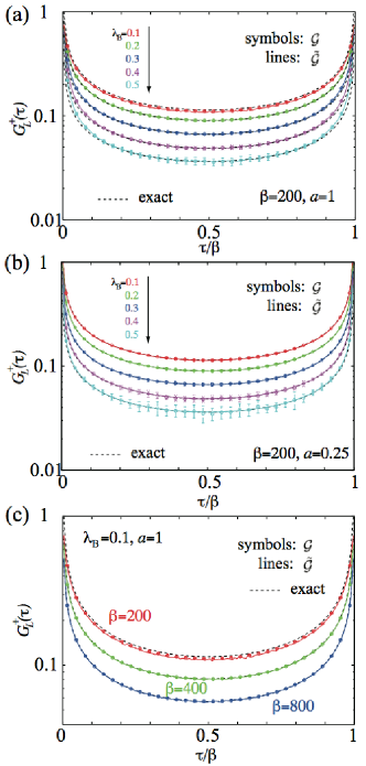
Figure 1: (Color online) GL+(τ)superscriptsubscript𝐺𝐿𝜏G_{L}^{+}(\tau) vs τ/β𝜏𝛽\tau/\beta for several coupling constants λB=0.1subscript𝜆𝐵0.1\lambda_{B}=0.1(top)-0.50.50.5(bottom) and inverse temperatures β𝛽\beta. The exact result (dashed line) is compared to two numerical methods [points with error bars: Eq. (43), solid lines: Eq. (45)]. A comparison of panel (a) (cutoff a=1𝑎1a=1) to panel (b) (cutoff a=0.25𝑎0.25a=0.25) shows that small deviations from the exact result vanish for small a𝑎a. Panel (c) shows that highly accurate results can be obtained even for very low T𝑇T.

In this subsection, we show the results for g=1𝑔1g=1, i.e., a system of noninteracting electrons. We compare the electron Green’s function obtained in the CTQMC and the exact results as follows:

GL+,ex(τ)=[s(τ)]121+π2λB2/v2,subscriptsuperscript𝐺ex𝐿𝜏superscriptdelimited-[]𝑠𝜏121superscript𝜋2superscriptsubscript𝜆𝐵2superscript𝑣2\displaystyle G^{+,\rm ex}_{L}(\tau)=\frac{\big{[}s(\tau)\big{]}^{-\frac{1}{2}}}{1+\pi^{2}\lambda_{B}^{2}/v^{2}}, (47)

which can be easily obtained from the equations of motion for the Green’s functions.

Figure 1 shows GL+(τ)subscriptsuperscript𝐺𝐿𝜏G^{+}_{L}(\tau) as a function of τ𝜏\tau for β=200𝛽200\beta=200 and several parameters λ𝜆\lambda and a𝑎a. In each plot, the exact result (dashed lines) and the result of the two methods described above are shown. The points with error bars (indicating the statistical error arising from the Monte Carlo sampling) are obtained from Eq. (43), while the solid lines have been calculated from Eq. (45) (the statistical error can be read off from the size of the noise in the curves). As one can see, the numerical data and the exact results are consistent with each other. More precisely, the Green’s functions are only identical in the limit a0𝑎0a\to 0 [we used this limit both in the derivation of the CTQMC approach and in Eq. (47)]. Figure 1 shows that tiny systematic deviations of the exact and the numerical result visible for a=1𝑎1a=1 become smaller than the noise for a=0.25𝑎0.25a=0.25. In the following, we will always use a=1𝑎1a=1 as the universal properties for Tv/amuch-less-than𝑇𝑣𝑎T\ll v/a and τa/vmuch-greater-than𝜏𝑎𝑣\tau\gg a/v discussed in the following are independent of the cutoff.

Figure 1 shows that highly accurate results are also obtained for low T𝑇T. Comparing the two computational methods (using the same computational time), we first note that both give reliable results. Which method is preferable depends in general both on the perturbation order and the type of binning in time used to extract data. For the parameter regime used in our calculations, we found the second approach to be more efficient. For very high orders of perturbation theory and small number of bins, however, the first approach can beat the second one in efficiency. In Sec. V.1, we will discuss that in regimes, where the nonlinearities are irrelevant (attractive interactions), the second method is inefficient.

IV.1.3 Universal scaling function for electron Green’s function

The main prediction of Kane and Fisher KF is that for repulsive interactions, g<1𝑔1g<1, even a weak impurity effectively cuts the chain: Electrons scatter so efficiently from the slowly decaying Friedel oscillations that for T0𝑇0T\to 0 and at the Fermi energy one obtains perfect reflection. The fact that the impurity cuts the quantum wire can also be measured by tunneling spectroscopy, i.e., by considering the local Green’s function close to the impurity. Based on the assumption that the wire is perfectly cut by the impurity, one expects for T=0𝑇0T=0,

GL+(τ)τ1/(2g),similar-tosubscriptsuperscript𝐺𝐿𝜏superscript𝜏12𝑔G^{+}_{L}(\tau\to\infty)\sim\tau^{-1/(2g)}, (48)

as has been derived by Furusaki Furusaki . This prediction can be checked analytically for g=1/2𝑔12g=1/2, where an exact analytic result can be derived Delft . Equation (48) should be compared to GL+(τ)τg/2similar-tosubscriptsuperscript𝐺𝐿𝜏superscript𝜏𝑔2G^{+}_{L}(\tau\to\infty)\sim\tau^{-g/2} obtained for λB=0subscript𝜆𝐵0\lambda_{B}=0, in the absence of the impurity.

Note that for the computation of the physical electron Green’s function one has to consider a further contribution, GLR(τ)=TτψL(τ)ψR(0)subscript𝐺𝐿𝑅𝜏delimited-⟨⟩subscript𝑇𝜏subscript𝜓𝐿𝜏superscriptsubscript𝜓𝑅0G_{LR}(\tau)=-\langle T_{\tau}\psi_{L}(\tau)\psi_{R}^{\dagger}(0)\rangle, in addition to GL(τ)subscript𝐺𝐿𝜏G_{L}(\tau). It is possible to calculate GLR(τ)subscript𝐺𝐿𝑅𝜏G_{LR}(\tau) using our approach, but we do not discuss it here for simplicity.

From general scaling arguments and the analysis of Kane and Fisher KF , one expects for a weak potential scatterer (small λBsubscript𝜆𝐵\lambda_{B}) a crossover from GL+(τ)τg/2similar-tosubscriptsuperscript𝐺𝐿𝜏superscript𝜏𝑔2G^{+}_{L}(\tau\to\infty)\sim\tau^{-g/2} to GL+(τ)τ1/(2g)similar-tosubscriptsuperscript𝐺𝐿𝜏superscript𝜏12𝑔G^{+}_{L}(\tau\to\infty)\sim\tau^{-1/(2g)} described by a universal (but g𝑔g-dependent) scaling function gsubscript𝑔\mathcal{F}_{g},

GL+(τ)[s(τ)]g/2g(Tτ,T/T),superscriptsubscript𝐺𝐿𝜏superscriptdelimited-[]𝑠𝜏𝑔2subscript𝑔superscript𝑇𝜏𝑇superscript𝑇\displaystyle G_{L}^{+}(\tau)\approx[s(\tau)]^{-g/2}\,{\mathcal{F}}_{g}(\,T^{*}\tau\,,T/T^{*}), (49)

where [s(τ)]g/2superscriptdelimited-[]𝑠𝜏𝑔2[s(\tau)]^{-g/2} is the Green’s function for λB=0subscript𝜆𝐵0\lambda_{B}=0, see Eq. (LABEL:VVVV). All dependence on the strength λBsubscript𝜆𝐵\lambda_{B} of the impurity potential is thereby encoded in the characteristic energy scale Tsuperscript𝑇T^{*} with

T=va(λBv)1/(1g),superscript𝑇𝑣𝑎superscriptsubscript𝜆𝐵𝑣11𝑔T^{*}=\frac{v}{a}\left(\frac{\lambda_{B}}{v}\right)^{1/(1-g)}, (50)

for small λBsubscript𝜆𝐵\lambda_{B}. The universal scaling form (49) is expected to be valid whenever Tsuperscript𝑇T^{*} is much smaller than the cutoff energy v/a𝑣𝑎v/a. For T=0𝑇0T=0 and weak λBsubscript𝜆𝐵\lambda_{B}, the short time dynamics is determined by the noninteracting result, g(x0,0)=1subscript𝑔𝑥001{\mathcal{F}}_{g}(x\to 0,0)=1, while g(x,0)x(g1/g)/2proportional-tosubscript𝑔𝑥0superscript𝑥𝑔1𝑔2{\mathcal{F}}_{g}(x\to\infty,0)\propto x^{(g-1/g)/2}, see Eq. (48).

In the following, we show our CTQMC results, which confirm the expected behavior and allow us to calculate the full scaling function describing the crossover from weak to strong coupling. To our knowledge, this is the first demonstration of the numerically-exact Green’s function in this model.

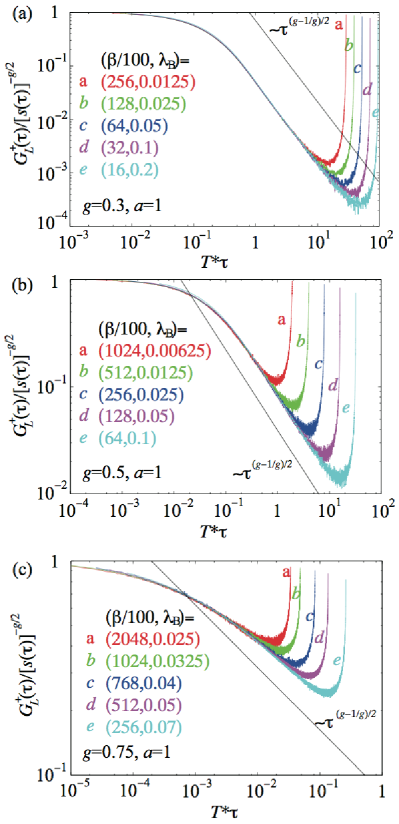
Figure 2 shows GL+(τ)/[s(τ)]g/2subscriptsuperscript𝐺𝐿𝜏superscriptdelimited-[]𝑠𝜏𝑔2G^{+}_{L}(\tau)/[s(\tau)]^{-g/2} versus Tτsuperscript𝑇𝜏T^{*}\tau for several parameter sets (β,λB)𝛽subscript𝜆𝐵(\beta,\lambda_{B}) and (a) g=0.3𝑔0.3g=0.3, (b) g=0.5𝑔0.5g=0.5, and (c) g=0.75𝑔0.75g=0.75 for various temperatures T𝑇T. Our numerical results reproduce the analytically expected behaviors: First, for wide ranges of λBsubscript𝜆𝐵\lambda_{B} the curves scale on top of each other (we have not used an appropriately rescaled temperature, therefore the upturns occur at different points). Second, we obtain the analytically expected asymptotic behavior with g(x0,0)=1subscript𝑔𝑥001{\mathcal{F}}_{g}(x\to 0,0)=1, while g(x,0)x(g1/g)/2proportional-tosubscript𝑔𝑥0superscript𝑥𝑔1𝑔2{\mathcal{F}}_{g}(x\to\infty,0)\propto x^{(g-1/g)/2}, see Eq. (48). Third, our result provides the full crossover function from weak to strong coupling.
Refer to caption
Figure 2: (Color online) GL+(τ)/[s(τ)]g/2superscriptsubscript𝐺𝐿𝜏superscriptdelimited-[]𝑠𝜏𝑔2G_{L}^{+}(\tau)/[s(\tau)]^{-g/2} versus Tτsuperscript𝑇𝜏T^{*}\tau for various parameter sets (β,λB)𝛽subscript𝜆𝐵(\beta,\lambda_{B}), a=1𝑎1a=1 and (a) g=0.3𝑔0.3g=0.3, (b) g=0.5𝑔0.5g=0.5, and (c) g=0.75𝑔0.75g=0.75. Straight lines show the τ(g1/g)/2superscript𝜏𝑔1𝑔2\tau^{(g-1/g)/2} dependence expected from the fixed point where the impurity cuts the chain (the factor τg/2superscript𝜏𝑔2\tau^{g/2} originates from the asymptotic form of [s(τ)]g/2superscriptdelimited-[]𝑠𝜏𝑔2[s(\tau)]^{-g/2}).
Refer to caption
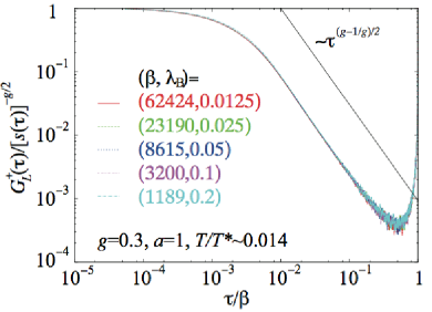
Figure 3: (Color online) GL+(τ)/[s(τ)]g/2superscriptsubscript𝐺𝐿𝜏superscriptdelimited-[]𝑠𝜏𝑔2G_{L}^{+}(\tau)/[s(\tau)]^{-g/2} vs τ/β𝜏𝛽\tau/\beta for a=1𝑎1a=1 and various parameters (β,λB)𝛽subscript𝜆𝐵(\beta,\lambda_{B}) keeping the ratio T/T0.014similar-to-or-equals𝑇superscript𝑇0.014T/T^{*}\simeq 0.014 fixed.

To prove that scaling works also at finite T𝑇T, we show in Fig. 3 GL+(τ)/[s(τ)]g/2subscriptsuperscript𝐺𝐿𝜏superscriptdelimited-[]𝑠𝜏𝑔2G^{+}_{L}(\tau)/[s(\tau)]^{-g/2} as a function of τ/β𝜏𝛽\tau/\beta for a wide range of coupling constants λBsubscript𝜆𝐵\lambda_{B} using a fixed ratio of T/T0.014𝑇superscript𝑇0.014T/T^{*}\approx 0.014. The perfect collapse of the data shows that temperature only enters in the combination T/T𝑇superscript𝑇T/T^{*} as predicted by Eq. (49).

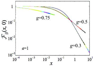
Finally, we show the T=0𝑇0T=0 scaling functions g(x,0)subscript𝑔𝑥0{\mathcal{F}}_{g}(x,0) for g=0.75𝑔0.75g=0.75, g=0.5𝑔0.5g=0.5, and g=0.3𝑔0.3g=0.3 in Fig. 4. The T=0𝑇0T=0 curves can simply be obtained from the small τ𝜏\tau data (we use τ/β<1/6𝜏𝛽16\tau/\beta<1/6) shown in Fig. 2, which are independent of β𝛽\beta within the scatter of the curve. For g𝑔g close to 111, Tsuperscript𝑇T^{*} becomes exponentially small and it becomes more difficult to extract the low T𝑇T and long τ𝜏\tau results.

Refer to caption
Figure 4: (Color online) g(x,0)subscript𝑔𝑥0{\mathcal{F}}_{g}(x,0) vs x𝑥x for g=0.75𝑔0.75g=0.75, g=0.5𝑔0.5g=0.5, and g=0.3𝑔0.3g=0.3 with a=1𝑎1a=1. Data for τ/β<1/6𝜏𝛽16\tau/\beta<1/6 of each of the lines in Fig. 2 are used in order to extract the T=0𝑇0T=0 limit.

IV.2 XXZ Kondo model in helical liquids

Along edges of two-dimensional topological insulators, a special one-dimensional electron system is realized Wu . Namely right- and left-moving electrons have opposite spin polarizations, up and down, respectively. The topological protection of these edge channels is reflected by unusual scattering properties: due to time-reversal symmetry a static potential cannot scatter a right-moving spin-up electron into a left-moving spin-down electron.

The situation differs in the presence of a magnetic impurity. Using a spin-flip process, a right mover can be converted in a left mover (and vice versa) due to the exchange interaction with the quantum impurity. Therefore, it is an interesting problem to study magnetic quantum impurities at the edge of a topological insulator to investigate whether and how topological protection is affected by their presence.

In this subsection, we examine the spin-1/2 XXZ Kondo model Wu ; Mac0 ; Mac . We restrict our analysis to the case where the total spin in the z𝑧z direction is conserved. Although this symmetry is broken in real materials, e.g., by Rashba interactions Erik ; Alt , it is important to clarify also the basic properties of this simplified problem. Note that the transport properties in the presence and absence of this symmetry qualitatively differ as the current in a helical edge state (proportional to NNsubscript𝑁subscript𝑁N_{\uparrow}-N_{\downarrow}) can only degrade by processes where spin conservation is violated.

We will use different units from those in the previous subsection, and use the energy unit v/ξ=1𝑣𝜉1v/\xi=1 for all g𝑔g and ξ=1𝜉1\xi=1 as a unit of length, in order to use the same high-energy cutoff as in previous studies Wu ; Mac0 ; Mac . The main results in this subsection are the phase diagram in g𝑔g-λBsubscript𝜆𝐵\lambda_{B} plane, which has been discussed perturbatively Wu ; Mac and the numerically-exact time and temperature dependence of the spin-spin correlation functions for general interaction parameters.

IV.2.1 Model

For XXZ Kondo model, X^Fσsuperscriptsubscript^𝑋𝐹𝜎\hat{X}_{F}^{\sigma} and X^Bsubscript^𝑋𝐵\hat{X}_{B} in Eqs. (11) and (12) are given as

X^F+=S^z,X^F=1,andX^B=S^.formulae-sequencesuperscriptsubscript^𝑋𝐹superscript^𝑆𝑧formulae-sequencesuperscriptsubscript^𝑋𝐹1andsubscript^𝑋𝐵superscript^𝑆\displaystyle\hat{X}_{F}^{+}=\hat{S}^{z},\quad\hat{X}_{F}^{-}=1,\quad{\rm and}\ \ \ \hat{X}_{B}=\hat{S}^{-}. (51)

We have used a slightly different quantization axis of the impurity spin from in Refs. Mac0 ; Mac : S^zS^zsubscript^𝑆𝑧subscript^𝑆𝑧\hat{S}_{z}\leftrightarrow-\hat{S}_{z} and S^±S^superscript^𝑆plus-or-minussuperscript^𝑆minus-or-plus\hat{S}^{\pm}\leftrightarrow\hat{S}^{\mp}. Since VFsuperscriptsubscript𝑉𝐹V_{F}^{-} term is a pure potential scattering in the charge sector and equivalently ΦsubscriptΦ\Phi_{-} sector, this does not affect the CTQMC and the following discussions, we will concentrate on the Φ+subscriptΦ\Phi_{+} sector, VF++VBsuperscriptsubscript𝑉𝐹subscript𝑉𝐵V_{F}^{+}+V_{B}, hereafter.

First, we write the Hamiltonian in the bosonization basis

H𝐻\displaystyle H =\displaystyle= H1Dsubscript𝐻1𝐷\displaystyle H_{1D} (52)
+λF2/gxΦ+(0)S^z+λ~BFLFRV^+2g(Φ+)S^subscript𝜆𝐹2𝑔subscript𝑥subscriptΦ0superscript^𝑆𝑧subscript~𝜆𝐵superscriptsubscript𝐹𝐿subscript𝐹𝑅subscript^𝑉2𝑔subscriptΦsuperscript^𝑆\displaystyle+\lambda_{F}\sqrt{2/g}\partial_{x}\Phi_{+}(0)\hat{S}^{z}+\tilde{\lambda}_{B}F_{L}^{\dagger}F_{R}\hat{V}_{+\sqrt{2g}}(\Phi_{+})\hat{S}^{-}
+λ~BFRFLV^2g(Φ+)S^+,subscriptsuperscript~𝜆𝐵superscriptsubscript𝐹𝑅subscript𝐹𝐿subscript^𝑉2𝑔subscriptΦsuperscript^𝑆\displaystyle+\tilde{\lambda}^{*}_{B}F_{R}^{\dagger}F_{L}\hat{V}_{-\sqrt{2g}}(\Phi_{+})\hat{S}^{+},

where λF=Jza/2πsubscript𝜆𝐹subscript𝐽𝑧𝑎2𝜋\lambda_{F}=J_{z}a/2\pi describes the coupling of the z𝑧z-component of the spin, while λB=Ja/2πsubscript𝜆𝐵subscript𝐽perpendicular-to𝑎2𝜋\lambda_{B}=J_{\perp}a/2\pi parametrizes the strength of spin-flip terms Mac0 .

For the CTQMC, it is useful to transform H𝐻H via a unitary transformation U^^𝑈\hat{U} Mac ,

U^exp[i2gλFgvΦ+(0)S^z].^𝑈𝑖2𝑔subscript𝜆𝐹𝑔𝑣subscriptΦ0superscript^𝑆𝑧\hat{U}\equiv\exp\Bigg{[}i\frac{\sqrt{2g}\lambda_{F}}{gv}\Phi_{+}(0)\hat{S}^{z}\Bigg{]}. (53)

This erases the λFsubscript𝜆𝐹\lambda_{F} term in Eq. (52), since

U^H1DU^=H1D2gλFgvvS^zxΦ+(0).^𝑈subscript𝐻1𝐷superscript^𝑈subscript𝐻1𝐷2𝑔subscript𝜆𝐹𝑔𝑣𝑣superscript^𝑆𝑧subscript𝑥subscriptΦ0\hat{U}H_{1D}\hat{U}^{\dagger}=H_{1D}-\frac{\sqrt{2g}\lambda_{F}}{gv}\cdot v\hat{S}^{z}\partial_{x}\Phi_{+}(0). (54)

Thus, the Hamiltonian is transformed to

U^HU^^𝑈𝐻superscript^𝑈\displaystyle\hat{U}H\hat{U}^{\dagger} =\displaystyle= H1D+λBFLFRV^+λ(Φ+)S^subscript𝐻1𝐷subscriptsuperscript𝜆𝐵superscriptsubscript𝐹𝐿subscript𝐹𝑅subscript^𝑉superscript𝜆subscriptΦsuperscript^𝑆\displaystyle H_{1D}+{\lambda}^{\prime}_{B}F_{L}^{\dagger}F_{R}\hat{V}_{+\lambda^{\prime}}(\Phi_{+})\hat{S}^{-} (55)
+λBFRFLV^λ(Φ+)S^+,subscriptsuperscript𝜆𝐵superscriptsubscript𝐹𝑅subscript𝐹𝐿subscript^𝑉superscript𝜆subscriptΦsuperscript^𝑆\displaystyle+{\lambda^{\prime*}_{B}}F_{R}^{\dagger}F_{L}\hat{V}_{-\lambda^{\prime}}(\Phi_{+})\hat{S}^{+},

with λ=g2/gsuperscript𝜆superscript𝑔2𝑔\lambda^{\prime}=g^{\prime}\sqrt{2/g} and λB=λBag2/g1subscriptsuperscript𝜆𝐵subscript𝜆𝐵superscript𝑎superscriptsuperscript𝑔2𝑔1\lambda^{\prime}_{B}=\lambda_{B}a^{{g^{\prime}}^{2}/g-1}, where gsuperscript𝑔g^{\prime} is defined as

g=gλF/v.superscript𝑔𝑔subscript𝜆𝐹𝑣\displaystyle g^{\prime}=g-\lambda_{F}/v. (56)

As will be discussed in Appendix B, it is sufficient to consider cases for λFgvsubscript𝜆𝐹𝑔𝑣\lambda_{F}\leq gv, i.e., λ0superscript𝜆0\lambda^{\prime}\geq 0.

The CTQMC algorithm for this model is similar to that for the Kane-Fisher model. Indeed, an exact relation between the partition functions of the two models is known FendleyZ . Only even N=2k𝑁2𝑘N=2k order terms remain finite due to the fact that the impurity spin is 1/2, i.e., S^+S^+=S^S^=0superscript^𝑆superscript^𝑆superscript^𝑆superscript^𝑆0\hat{S}^{+}\hat{S}^{+}=\hat{S}^{-}\hat{S}^{-}=0 and/or the total fermion number conservation. This also restricts configuration space for the impurity spin in Z𝑍Z. We just need to generate configurations in which S+superscript𝑆S^{+} and Ssuperscript𝑆S^{-} appear alternatively: S^±(τ1)S^(τ2)S^±(τ3)superscript^𝑆plus-or-minussubscript𝜏1superscript^𝑆minus-or-plussubscript𝜏2superscript^𝑆plus-or-minussubscript𝜏3\hat{S}^{\pm}(\tau_{1})\hat{S}^{\mp}(\tau_{2})\hat{S}^{\pm}(\tau_{3})\cdots. Thus, we can use algorithm similar to the “segment” representation used in the Anderson model, which accelerates the acceptance rate in the MC samplings Werner .

IV.2.2 Spin-spin correlation function

In this subsection, we explain how to calculate the dynamical spin-spin correlation functions.

First, let us discuss the transverse local spin susceptibility, χ(τij)[χ+(τij)+χ+(τij)]/2superscript𝜒perpendicular-tosubscript𝜏𝑖𝑗delimited-[]superscript𝜒absentsubscript𝜏𝑖𝑗superscript𝜒absentsubscript𝜏𝑖𝑗2\chi^{\perp}(\tau_{ij})\equiv[\chi^{+-}(\tau_{ij})+\chi^{-+}(\tau_{ij})]/2, where χ±(τij)superscript𝜒plus-or-minusabsentminus-or-plussubscript𝜏𝑖𝑗\chi^{\pm\mp}(\tau_{ij}) is defined as

χ+(τij)TτS^+(τi)S^(τj).superscript𝜒absentsubscript𝜏𝑖𝑗delimited-⟨⟩subscript𝑇𝜏superscript^𝑆subscript𝜏𝑖superscript^𝑆subscript𝜏𝑗\displaystyle\chi^{+-}(\tau_{ij})\equiv\langle T_{\tau}\hat{S}^{+}(\tau_{i})\hat{S}^{-}(\tau_{j})\rangle. (57)

Noting that U^S^±U^=e±i2gλF/(gv)Φ+(0)S^±^𝑈superscript^𝑆plus-or-minussuperscript^𝑈superscript𝑒plus-or-minus𝑖2𝑔subscript𝜆𝐹𝑔𝑣subscriptΦ0superscript^𝑆plus-or-minus\hat{U}\hat{S}^{\pm}\hat{U}^{\dagger}=e^{\pm i\sqrt{2g}\lambda_{F}/(gv)\Phi_{+}(0)}\hat{S}^{\pm}, we can calculate

χ+(τ)=1βijkij[δ(ττij)+δ(β+τijτ)],superscript𝜒absent𝜏1𝛽delimited-⟨⟩superscriptsubscript𝑖𝑗𝑘subscript𝑖𝑗delimited-[]𝛿𝜏subscript𝜏𝑖𝑗𝛿𝛽subscript𝜏𝑖𝑗𝜏\chi^{+-}(\tau)=\frac{1}{\beta}\left\langle\sum_{ij}^{k}{\mathcal{M}}_{ij}\Big{[}\delta(\tau-\tau_{ij})+\delta(\beta+\tau_{ij}-\tau)\Big{]}\right\rangle,\ \ \ (58)

by sampling the following quantity:

ijsubscript𝑖𝑗\displaystyle{\mathcal{M}}_{ij}\! =\displaystyle= a2g(λFgv)2|λB|2[s(τij)]2λFv|detS^k1{ττi,τj+}detS^k{τ}|2gsuperscript𝑎2𝑔superscriptsubscript𝜆𝐹𝑔𝑣2superscriptsubscriptsuperscript𝜆𝐵2superscriptdelimited-[]𝑠subscript𝜏𝑖𝑗2subscript𝜆𝐹𝑣superscriptdetsubscript^𝑆𝑘1symmetric-difference𝜏superscriptsubscript𝜏𝑖superscriptsubscript𝜏𝑗detsubscript^𝑆𝑘𝜏2superscript𝑔\displaystyle\!\frac{a^{2g(\frac{\lambda_{F}}{gv})^{2}}}{|\lambda^{\prime}_{B}|^{2}}\big{[}s(\tau_{ij})\big{]}^{-\frac{2\lambda_{F}}{v}}\Bigg{|}\frac{{\rm det}\hat{S}_{k-1}\{\tau\ominus\tau_{i}^{-},\tau_{j}^{+}\}}{{\rm det}\hat{S}_{k}\{\tau\}}\Bigg{|}^{2g^{\prime}} (59)
=\displaystyle= a2g(λFgv)2|λB|2[s(τij)]2λFv|(S^1{τ})ji|2g,superscript𝑎2𝑔superscriptsubscript𝜆𝐹𝑔𝑣2superscriptsubscriptsuperscript𝜆𝐵2superscriptdelimited-[]𝑠subscript𝜏𝑖𝑗2subscript𝜆𝐹𝑣superscriptsubscriptsuperscript^𝑆1𝜏𝑗𝑖2superscript𝑔\displaystyle\frac{a^{2g(\frac{\lambda_{F}}{gv})^{2}}}{|\lambda^{\prime}_{B}|^{2}}\big{[}s(\tau_{ij})\big{]}^{-\frac{2\lambda_{F}}{v}}\Big{|}(\hat{S}^{-1}\{\tau\})_{ji}\Big{|}^{2g^{\prime}},

where τisubscript𝜏𝑖\tau_{i} and τjsubscript𝜏𝑗\tau_{j} are chosen in a given snapshot {τ}𝜏\{\tau\} at the 2k2𝑘2kth order as in Eq. (45) and the corresponding vertex operators at τisubscript𝜏𝑖\tau_{i} and τjsubscript𝜏𝑗\tau_{j} should have λi=λ<0subscript𝜆𝑖superscript𝜆0\lambda_{i}=-\lambda^{\prime}<0 and λj=λ>0subscript𝜆𝑗superscript𝜆0\lambda_{j}=\lambda^{\prime}>0, respectively. For χ+(τij)superscript𝜒absentsubscript𝜏𝑖𝑗\chi^{-+}(\tau_{ij}), the same expression holds with regarding now λi>0subscript𝜆𝑖0\lambda_{i}>0 and λj<0subscript𝜆𝑗0\lambda_{j}<0. We also use symmetry properties χ±(|τ|)=χ±(β|τ|)superscript𝜒plus-or-minusabsentminus-or-plus𝜏superscript𝜒plus-or-minusabsentminus-or-plus𝛽𝜏\chi^{\pm\mp}(-|\tau|)=\chi^{\pm\mp}(\beta-|\tau|) to obtain results for 0τβ0𝜏𝛽0\leq\tau\leq\beta. ijsubscript𝑖𝑗{\mathcal{M}}_{ij} is, indeed, derived in an almost identical way as in Appendix A.2.

Second, as US^zU=S^z𝑈superscript^𝑆𝑧superscript𝑈superscript^𝑆𝑧U\hat{S}^{z}U^{\dagger}=\hat{S}^{z}, the longitudinal spin susceptibility is directly evaluated as

χz(τij)=superscript𝜒𝑧subscript𝜏𝑖𝑗absent\displaystyle\chi^{z}(\tau_{ij})=
1NMCi=1NMCS^±(τ1)S^z(τi)S^z(τj)S^(τ2k)impS^±(τ1)S^(τ2k)imp.1subscript𝑁MCsuperscriptsubscript𝑖1subscript𝑁MCsubscriptdelimited-⟨⟩superscript^𝑆plus-or-minussubscript𝜏1superscript^𝑆𝑧subscript𝜏𝑖superscript^𝑆𝑧subscript𝜏𝑗superscript^𝑆minus-or-plussubscript𝜏2𝑘impsubscriptdelimited-⟨⟩superscript^𝑆plus-or-minussubscript𝜏1superscript^𝑆minus-or-plussubscript𝜏2𝑘imp\displaystyle\frac{1}{N_{\rm MC}}\sum_{i=1}^{N_{\rm MC}}\frac{\langle\hat{S}^{\pm}(\tau_{1})\cdots\hat{S}^{z}(\tau_{i})\cdots\hat{S}^{z}(\tau_{j})\cdots\hat{S}^{\mp}(\tau_{2k})\rangle_{\rm imp}}{\langle\hat{S}^{\pm}(\tau_{1})\cdots\hat{S}^{\mp}(\tau_{2k})\rangle_{\rm imp}}.\ \ \ \ \
(60)

This is possible because the operator S^zsubscript^𝑆𝑧\hat{S}_{z} does not alter any quantum numbers along the imaginary time axis in CTQMC. In contrast, the transverse susceptibility can be calculated only through the more complicated Eq. (59) [if one would replace S^z(τi,j)superscript^𝑆𝑧subscript𝜏𝑖𝑗\hat{S}^{z}(\tau_{i,j}) by S^±(τi,j)superscript^𝑆plus-or-minussubscript𝜏𝑖𝑗\hat{S}^{\pm}(\tau_{i,j}) in Eq. (60), one would get just zero, since the inserted S^±(τi,j)superscript^𝑆plus-or-minussubscript𝜏𝑖𝑗\hat{S}^{\pm}(\tau_{i,j}) are always next to S^±(τα)superscript^𝑆plus-or-minussubscript𝜏𝛼\hat{S}^{\pm}(\tau_{\alpha}) with τα{τ}]\tau_{\alpha}\in\{\tau\}].

IV.2.3 SU(2) check for g=1𝑔1g=1 and λF=λBsubscript𝜆𝐹subscript𝜆𝐵\lambda_{F}=\lambda_{B}

Interactions at the edge of the quantum wire destroy even for λF=λBsubscript𝜆𝐹subscript𝜆𝐵\lambda_{F}=\lambda_{B} the SU(2) spin symmetry. In the noninteracting electron limit (g=1𝑔1g=1), however, the algorithm has to recover SU(2) symmetry for λF=λBsubscript𝜆𝐹subscript𝜆𝐵\lambda_{F}=\lambda_{B}. As the algorithm treats spin-flip and nonflip terms very differently, it is a nontrivial check of the numerical data to see whether 2χz(τ)=χ(τ)2superscript𝜒𝑧𝜏superscript𝜒perpendicular-to𝜏2\chi^{z}(\tau)=\chi^{\perp}(\tau).

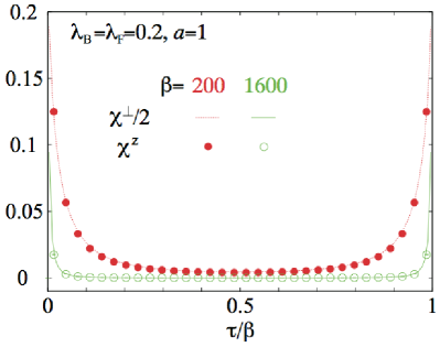
Figure 5 shows χz,(τ)superscript𝜒𝑧perpendicular-to𝜏\chi^{z,\perp}(\tau) versus τ/β𝜏𝛽\tau/\beta for λF=λB=0.2subscript𝜆𝐹subscript𝜆𝐵0.2\lambda_{F}=\lambda_{B}=0.2 and a=1𝑎1a=1. As one can see, the relation 2χz(τ)=χ(τ)2superscript𝜒𝑧𝜏superscript𝜒perpendicular-to𝜏2\chi^{z}(\tau)=\chi^{\perp}(\tau) holds well. The intrinsic SU(2) symmetry breaking in the Abelian bosonization in our scheme leads to a small similar-to\sim10 % deviations from unity for χ(τ)/[2χz(τ)]superscript𝜒perpendicular-to𝜏delimited-[]2superscript𝜒𝑧𝜏\chi^{\perp}(\tau)/[2\chi^{z}(\tau)] for a=1𝑎1a=1. These errors do not alter the asymptotic behaviors for τ1much-greater-than𝜏1\tau\gg 1 and we have checked that the expected results χz,(τ)τ2similar-tosuperscript𝜒𝑧perpendicular-to𝜏superscript𝜏2\chi^{z,\perp}(\tau)\sim\tau^{-2} for g=1𝑔1g=1 are reproduced (see also Figs. 8 and 9).
Refer to caption
Figure 5: (Color online) Comparison between χ(τ)/2superscript𝜒perpendicular-to𝜏2\chi^{\perp}(\tau)/2 and χz(τ)superscript𝜒𝑧𝜏\chi^{z}(\tau) as a function of τ𝜏\tau for λF=λB=0.2subscript𝜆𝐹subscript𝜆𝐵0.2\lambda_{F}=\lambda_{B}=0.2, a=1𝑎1a=1, and β=200𝛽200\beta=200 and 160016001600.

IV.2.4 Phase diagram

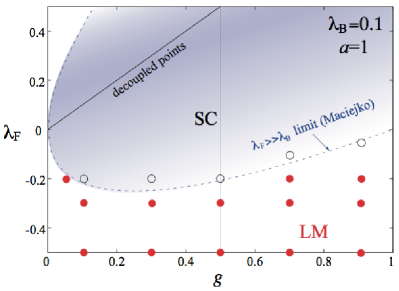
Before starting detailed analysis, we show in Fig. 6 the global phase diagram in the plane spanned by λFsubscript𝜆𝐹\lambda_{F} and g𝑔g for fixed λB=0.1subscript𝜆𝐵0.1\lambda_{B}=0.1. As pointed out in the previous studies Mac , there are two phases: the screened phase (SC) where the Kondo effect leads to a screening of the impurity and the local moment (LM) phase where spin-flips are completely suppressed for T0𝑇0T\to 0. The phase boundary for λB=0.1subscript𝜆𝐵0.1\lambda_{B}=0.1 is well described by the recent renormalization group results for λBλFmuch-less-thansubscript𝜆𝐵subscript𝜆𝐹\lambda_{B}\ll\lambda_{F} represented by the dashed line Mac . As discussed by Maciejko Mac and also as discussed in Appendix B, the system is symmetric at the solvable “decoupled points” at λF=gvsubscript𝜆𝐹𝑔𝑣\lambda_{F}=gv and the system for λF>gvsubscript𝜆𝐹𝑔𝑣\lambda_{F}>gv can be mapped to that for 2gvλB<gv2𝑔𝑣subscript𝜆𝐵𝑔𝑣2gv-\lambda_{B}<gv, and vice versa. Thus, we have only examined the lower part of the boundary in Fig. 6.

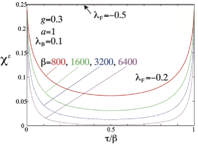
The two phases are easily distinguished by the temperature dependence of χz(τ)superscript𝜒𝑧𝜏\chi^{z}(\tau) . For example, Fig. 7 shows the typical behavior of the two phases for g=0.3𝑔0.3g=0.3. For the LM phase (λF=0.5subscript𝜆𝐹0.5\lambda_{F}=-0.5), χz(τ)superscript𝜒𝑧𝜏\chi^{z}(\tau) is large and almost τ𝜏\tau-independent. Also the T𝑇T variations are not noticeable on the the scale of the plot: the impurity spin is almost free and the spin-flips are strongly suppressed. In contrast, in the SC phase, λF=0.2subscript𝜆𝐹0.2\lambda_{F}=-0.2, χz(τ)superscript𝜒𝑧𝜏\chi^{z}(\tau) shows a strong temperature and τ𝜏\tau dependence, which reflects screening processes due to the conduction electrons. In the next subsection, we will discuss the low-temperature behaviors of the spin-spin correlation functions in the SC phase.
Refer to caption
Figure 6: (Color online) Phase diagram as a function of the TL parameter g𝑔g and the size of the coupling of the z𝑧z component of the exchange coupling λFsubscript𝜆𝐹\lambda_{F} for a fixed spin-flip rate λB=0.1subscript𝜆𝐵0.1\lambda_{B}=0.1 and a=1𝑎1a=1. Open (filled) circles indicate the screened (local-moment) phase. For the SC phase, points inside the phase are not indicated and the SC phase is symmetric with respect to the variation of λFsubscript𝜆𝐹\lambda_{F} around the decoupled-point line (see Appendix B). The dashed line represents the phase boundary determined by the renormalization group analysis for λFλBmuch-greater-thansubscript𝜆𝐹subscript𝜆𝐵\lambda_{F}\gg\lambda_{B} Mac .
Refer to caption
Figure 7: (Color online) Longitudinal dynamical local spin susceptibility χz(τ)superscript𝜒𝑧𝜏\chi^{z}(\tau) vs τ/β𝜏𝛽\tau/\beta for λF<0subscript𝜆𝐹0\lambda_{F}<0 and λB=0.1subscript𝜆𝐵0.1\lambda_{B}=0.1, a=1𝑎1a=1, and β=800𝛽800\beta=800-640064006400.

IV.2.5 Dynamical local spin susceptibility

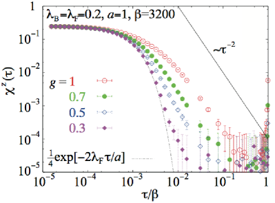
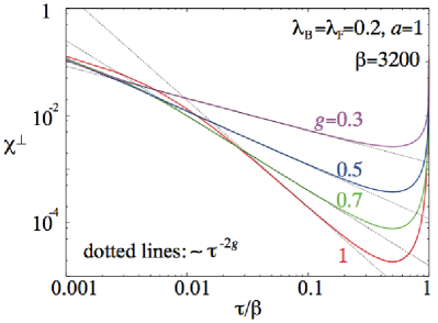
Figures 8 and 9 show the τ𝜏\tau dependence of the spin-spin correlation functions χ(τ)superscript𝜒perpendicular-to𝜏\chi^{\perp}(\tau) and χz(τ)superscript𝜒𝑧𝜏\chi^{z}(\tau), respectively, for λB,F=0.2subscript𝜆𝐵𝐹0.2\lambda_{B,F}=0.2, β=3200𝛽3200\beta=3200, and g=0.3𝑔0.3g=0.3, 0.50.50.5, 0.70.70.7, and 111. We find that the long-time asymptotic decay in the SC phase is given by

χ(τ)τ2g,similar-tosuperscript𝜒perpendicular-to𝜏superscript𝜏2𝑔\displaystyle\chi^{\perp}(\tau)\sim\tau^{-2g}, (61)

while

χz(τ)τ2forgλF/v.formulae-sequencesimilar-tosuperscript𝜒𝑧𝜏superscript𝜏2for𝑔subscript𝜆𝐹𝑣\displaystyle\chi^{z}(\tau)\sim\tau^{-2}\quad{\rm for}\ \ g\neq\lambda_{F}/v. (62)

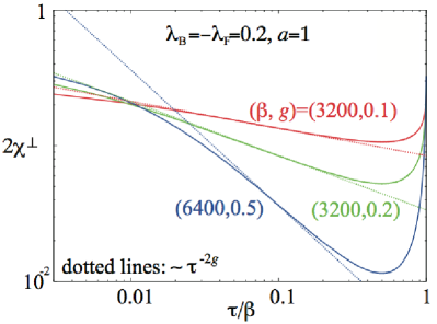
These τ𝜏\tau dependencies are also found for λF<0subscript𝜆𝐹0\lambda_{F}<0 as long as one remains in the SC phase as shown in Fig. 10, where χ(τ)superscript𝜒perpendicular-to𝜏\chi^{\perp}(\tau) are shown for simplicity. The characteristic energy scale becomes smaller and smaller as approaching the phase boundary (increasing g𝑔g). For g=0.5𝑔0.5g=0.5, β=6400𝛽6400\beta=6400 is still not sufficiently low to realize complete τ2gsuperscript𝜏2𝑔\tau^{-2g} dependence, while for smaller g𝑔g’s τ2gsuperscript𝜏2𝑔\tau^{-2g} dependence is realized already at β=3200𝛽3200\beta=3200.

Near the decoupled point at λF=gvsubscript𝜆𝐹𝑔𝑣\lambda_{F}=gv, the leading power-law decay τ2superscript𝜏2\tau^{-2} in χz(τ)superscript𝜒𝑧𝜏\chi^{z}(\tau) is suppressed and an exponential decay appears, while for χ(τ)superscript𝜒perpendicular-to𝜏\chi^{\perp}(\tau), there is no such contribution near the decoupled point. These results are consistent with the perturbative analysis in Appendix C. In the following, we will concentrate on the cases for λFgvsubscript𝜆𝐹𝑔𝑣\lambda_{F}\neq gv. Note that the exponent of χ(τ)superscript𝜒perpendicular-to𝜏\chi^{\perp}(\tau) is precisely given by that at the decoupled point, which is related to the scaling trajectory Mac .

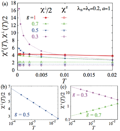
These asymptotic forms readily indicate that the local spin susceptibility χz,(T)superscript𝜒𝑧perpendicular-to𝑇\chi^{z,\perp}(T) exhibits

χz,(T)=0β𝑑τχz,(τ)T2Δz,1+const.,superscript𝜒𝑧perpendicular-to𝑇superscriptsubscript0𝛽differential-d𝜏superscript𝜒𝑧perpendicular-to𝜏similar-tosuperscript𝑇2subscriptΔ𝑧perpendicular-to1const\chi^{z,\perp}(T)=\int_{0}^{\beta}d\tau\chi^{z,\perp}(\tau)\sim T^{2\Delta_{z,\perp}-1}+{\rm const.}, (63)

where the constant part comes from the short-time cutoff. From our CTQMC results, the scaling dimensions Δz,subscriptΔ𝑧perpendicular-to\Delta_{z,\perp} at the screened fixed point are given by

Δz=1andΔ=g.formulae-sequencesubscriptΔ𝑧1andsubscriptΔperpendicular-to𝑔\displaystyle\Delta_{z}=1\quad{\rm and}\quad\Delta_{\perp}=g. (64)

This is the expected result: Applying a small magnetic field to the screened magnetic impurity is equivalent to applying a local magnetic field to the quantum wire without the magnetic impurity. This problem can directly be mapped to the Kane and Fisher problem investigated in the previous subsection. A magnetic field in the z𝑧z direction induces only forward scattering interaction, which is not renormalized, Δz=1subscriptΔ𝑧1\Delta_{z}=1, by the TLL interactions. In contrast, an infinitesimal transverse magnetic field is a relevant perturbation whose scaling dimension g𝑔g can be read off from Eq. (17).

For Δ=g=1/2subscriptΔperpendicular-to𝑔12\Delta_{\perp}=g=1/2, there are logarithmic corrections and

χ(T)lnT+const.forg=12.\chi^{\perp}(T)\sim-\ln T+{\rm const.}\quad{\rm for}\ g=\frac{1}{2}. (65)

Thus, the transverse spin susceptibility for g1/2𝑔12g\leq 1/2 diverges, while other cases and χsz(T)subscriptsuperscript𝜒𝑧𝑠𝑇\chi^{z}_{s}(T) stay constant at low temperatures.

These temperature dependencies are indeed obtained from a direct numerical integration of χsz,(τ)superscriptsubscript𝜒𝑠𝑧perpendicular-to𝜏\chi_{s}^{z,\perp}(\tau). Figure 11 shows χz,(T)superscript𝜒𝑧perpendicular-to𝑇\chi^{z,\perp}(T) for λB,F=0.2subscript𝜆𝐵𝐹0.2\lambda_{B,F}=0.2, a=1𝑎1a=1, g=1𝑔1g=1, 0.70.70.7, 0.50.50.5, and 0.30.30.3. For g=1𝑔1g=1, χ(T)=2χz(T)superscript𝜒perpendicular-to𝑇2superscript𝜒𝑧𝑇\chi^{\perp}(T)=2\chi^{z}(T) holds due to the SU(2) symmetry. For other values of g𝑔g’s, χ(T)2χz(T)superscript𝜒perpendicular-to𝑇2superscript𝜒𝑧𝑇\chi^{\perp}(T)\neq 2\chi^{z}(T). Figures 11 (b) and 11 (c) show that the susceptibilities follow the predicted power-law of Eq. (63) with high precision for g=0.7𝑔0.7g=0.7 and 0.30.30.3 and exhibit the expected logarithmic dependence for g=0.5𝑔0.5g=0.5, see Eq. (65). Note that for g=0.7𝑔0.7g=0.7 we plot [χ(0)χ(T)]/2delimited-[]superscript𝜒perpendicular-to0superscript𝜒perpendicular-to𝑇2[\chi^{\perp}(0)-\chi^{\perp}(T)]/2 with χ(0)/24.3superscript𝜒perpendicular-to024.3\chi^{\perp}(0)/2\approx 4.3 in order to analyze the subleading power-law dependence.
Refer to caption
Figure 8: (Color online) Transverse dynamical local spin susceptibility χ(τ)superscript𝜒perpendicular-to𝜏\chi^{\perp}(\tau) vs τ𝜏\tau for λF=λB=0.2subscript𝜆𝐹subscript𝜆𝐵0.2\lambda_{F}=\lambda_{B}=0.2, a=1𝑎1a=1, and β=3200𝛽3200\beta=3200. The dotted lines indicate 1/τ2gsimilar-toabsent1superscript𝜏2𝑔\sim 1/\tau^{2g}.
Refer to caption
Figure 9: (Color online) Longitudinal dynamical local spin susceptibility χz(τ)superscript𝜒𝑧𝜏\chi^{z}(\tau) vs τ𝜏\tau for λF=λB=0.2subscript𝜆𝐹subscript𝜆𝐵0.2\lambda_{F}=\lambda_{B}=0.2, a=1𝑎1a=1, and β=3200𝛽3200\beta=3200. The dashed line shows the exact result for gv=λF=0.2𝑔𝑣subscript𝜆𝐹0.2gv=\lambda_{F}=0.2: Eq. (86), and the line represents 1/τ21superscript𝜏21/\tau^{2}.
Refer to caption
Figure 10: (Color online) Transverse dynamical local spin susceptibility χ(τ)superscript𝜒perpendicular-to𝜏\chi^{\perp}(\tau) vs τ𝜏\tau for λF=λB=0.2subscript𝜆𝐹subscript𝜆𝐵0.2-\lambda_{F}=\lambda_{B}=0.2, a=1𝑎1a=1, and β=3200𝛽3200\beta=3200 and 640064006400. The dotted lines represent 1/τ2gsimilar-toabsent1superscript𝜏2𝑔\sim 1/\tau^{2g}.
Refer to caption
Figure 11: (Color online) (a) χz(T)superscript𝜒𝑧𝑇\chi^{z}(T) and χ(T)/2superscript𝜒perpendicular-to𝑇2\chi^{\perp}(T)/2 vs T𝑇T for λF=λB=0.2subscript𝜆𝐹subscript𝜆𝐵0.2\lambda_{F}=\lambda_{B}=0.2, a=1𝑎1a=1, and g=1𝑔1g=1, 0.70.70.7, 0.50.50.5, and 0.30.30.3. (b) χ(T)/2superscript𝜒perpendicular-to𝑇2\chi^{\perp}(T)/2 vs T𝑇T in the log scale for g=0.5𝑔0.5g=0.5. The line indicates the fit by 0.76log(T/0.66)0.76𝑇0.66-0.76\log(T/0.66). (c) χ(T)/2superscript𝜒perpendicular-to𝑇2\chi^{\perp}(T)/2 vs T𝑇T for g=0.7𝑔0.7g=0.7 and g=0.3𝑔0.3g=0.3 in the double-log scale. For g=0.7𝑔0.7g=0.7, 4.3χ(T)/24.3superscript𝜒perpendicular-to𝑇24.3-\chi^{\perp}(T)/2 is plotted and the line shows the fit by 7T0.47superscript𝑇0.47T^{0.4}. For g=0.3𝑔0.3g=0.3, the line indicates the fit by 0.396+0.66T0.40.3960.66superscript𝑇0.4-0.396+0.66T^{-0.4}.

V Discussions

In this section, we will discuss the reliability of some expressions for correlation functions in the “weak-coupling” fixed points and also discuss a possible extension of our method to more complex problems.

V.1 Correlation functions in the weak-coupling fixed points

For attractive interactions, g>1𝑔1g>1, in the Kane-Fisher model and for the local moment phase for the XXZ Kondo model, the nonlinear interactions are irrelevant and the system is therefore described by a weak coupling fixed point. In this regime, not only do the physical properties of the model completely differ (the impurity does not cut the chain and the local moment is not screened) but also the statistical properties of our Monte Carlo sampling change qualitatively. As a consequence, we find that the results based on the method defined by Eqs. (45) and (59) do not give reliable results, while, in contrast, the alternative approach, Eqs. (43) and (60), gives much better results. The reason Eqs. (45) and (59) are not efficient there would be the smallness of overlap between the important configurations for the partition function and those for the Green’s functions. This would be overcome by using a worm algorithm Gull . This is also the reason we use χz(τ)superscript𝜒𝑧𝜏\chi^{z}(\tau) (not affected by this problem) to identify the two phases in the XXZ Kondo model in Sec. IV.2.4.

V.2 Further applications

Here we discuss briefly further applications of our method for calculating other physical quantities for other models.

For impurity problems, the most important physical quantity is perhaps the conductance. It can naturally be computed within our scheme using that the current operator at x=0𝑥0x=0 is expressed by the time derivative of Φ+subscriptΦ\Phi_{+} as

j(x=0,τ)=ieg2πτΦ+(τ,x=0),𝑗𝑥0𝜏𝑖𝑒𝑔2𝜋subscript𝜏subscriptΦ𝜏𝑥0\displaystyle j(x=0,\tau)=i\frac{e\sqrt{g}}{2\pi}\partial_{\tau}\Phi_{+}(\tau,x=0), (66)

where e𝑒e is the elementary charge. The correlation function of j(0,τ)𝑗0𝜏j(0,\tau) can be effectively calculated in our CTQMC method, and, via analytic continuation to real frequency Jarrel , one can obtain the conductance. This can be done both for the Kane-Fisher and the XXZ Kondo problems. This approach is, however, beyond the scope of our work and will be published elsewhere future . Note that an analytic continuation to real frequencies is also needed to calculate, e.g., the tunneling density of states from our results for Green’s functions.

Our method can also be directly applied to other scattering problems, involving, for example, the backward scattering of pairs of fermions from nonmagnetic impurities at the edge of a two-dimensional topological insulator Mac ; Crepin . This problem is described by the same Hamiltonian as the Kane-Fisher model but, for example, the tunneling density of states, has to be computed from a different correlator.

In this paper, we have used two-component (L𝐿L and R𝑅R) fermionic models as a microscopic model for the bulk TLL. It is straightforward to apply this approach also to spin models or models of bosons in all cases where these models can be described by TLLs. Here one can use standard bosonization identities to map those problems to the ones considered in our paper. It is, however, important to keep track of Klein factors in such mappings. Since our approach fully relies on the noninteracting bosons in the bulk system, it should be emphasized that our method cannot manage interactions of the TLL bosons in the bulk (describing, e.g., Luther-Emery liquids LE or band-curvature effects).

It would also be highly interesting to study exotic Kondo models coupled to TLLs, which can, e.g., be realized using Majorana modes arising from topological edge states of superconducting islands Beri ; Beri2 ; Altland or by using two helical edges 2CKHL . With ultracold atoms, one can also realize Majorana edge mode coupled to a TLL Altman . Knowledge about the dynamics in such problems is not accessible so far, and thus, it is interesting to analyze them on the basis of the CTQMC developed in this paper.

Another technical challenge would be an analysis of impurity problems where two relevant operators compete with each other (arising, e.g., for Kondo models coupled to a helical edge when the spin in z𝑧z direction is not conserved) and also investigation of multiple and cluster impurities are highly nontrivial. While, for the cases discussed in this paper, no negative-sign problem occurred, this might not be the case for more complex realization involving several competing scattering channels.

VI Summary

In summary, we have demonstrated that the continuous-time quantum Monte Carlo method can successfully be applied to situations where a quantum impurity is coupled to an interacting one-dimensional quantum wire described by a Tomonaga-Luttinger liquid.

Our method is negative-sign free, which has been proved analytically, and thus, very low temperature calculations are possible as demonstrated. The coding can be realized by a straightforward extension of existing CTQMC codes for purely fermionic problems (without interactions in the environment) as the expression for δZ2k𝛿subscript𝑍2𝑘\delta Z_{2k} [Eq. (34)] are identical to those of fermionic systems apart from the exponent 2g2𝑔2g. This very simple modification from noninteracting electron system for the bulk part contains all the necessary information about interactions in the bulk system.

We have applied our algorithm to two models. One is the effect of a static scattering potential in a TLL discussed by Kane and Fisher in their classical work KF . The second is the XXZ Kondo model in the edge of two-dimensional topological insulators Wu ; Mac0 ; Mac .

For the Kane-Fisher model, we have demonstrated that the long-time asymptotic behavior of electron Green’s function is consistent with that predicted by Furusaki Furusaki . We have also computed the universal scaling function of the Green’s function for the first time.

As for the XXZ Kondo model, we have obtained the susceptibilities characterizing the two relevant fixed points: the decoupled local moment fixed point and the screened Kondo fixed point. The temperature dependence and the asymptotic time dependence are consistent with analytic predictions in the whole parameter regime.

The method introduced in this paper is flexible and can be applied to other models and used to study transport properties. We will report analyses of experimentally measurable quantities via analytic continuations and other interesting models in future publications.

Acknowledgment

The authors thank M. Garst and J. Kleinen for fruitful discussions. This work is supported by a Grant-in-Aid for Scientific Research (Grant No. 30456199) from the Japan Society for the Promotion of Science and by the center for Quantum Matter and Materials (QM2) of the University of Cologne. K. H. was supported by Yamada Science Foundation for his long-term stay at the University of Cologne. Some of the numerical calculations were done at the Supercomputer Center at ISSP, University of Tokyo.

References

  • (1) S. Tomonaga, Prog. Theor. Phys. 5, 544 (1950), J. M. Luttinger, J. Math. Phys. 4, 1154 (1963).
  • (2) T. Giamarchi, Quantum Physics in One Dimension, (Oxford University Press, Oxford, 2004).
  • (3) C. L. Kane and M. P. A. Fisher, Phys. Rev. Lett. 68, 1220 (1992); Phys. Rev. B 46, 15233 (1992).
  • (4) J. v. Delft and H. Schoeller, Ann. Pnys. (Leipzig) 7, 225 (1998).
  • (5) A. Furusaki, Phys. Rev. B 56, 9352 (1997).
  • (6) P. Fendley, H. Saleur, N. P. Wamer, Nucl. Phys. B430, 577 (1994), P. Fendley, A. W. W. Ludwig, and H. Saleur, Phys. Rev. Lett. 74, 3005 (1995), P. Fendley, F. Lesage, and H. Saleur, J. Stat. Phys. 85, 211 (1996).
  • (7) T. Enss, V. Meden, S. Andergassen, X. Barnabé-Thériault, W. Metzner, and K. Schönhammer, Phys. Rev. B 71, 155401 (2005).
  • (8) K. Moon, H. Yi, C. L. Kane, S. M. Girvin, and M. P. A. Fisher, Phys. Rev. Lett. 71, 4381 (1993).
  • (9) K. Leung, R. Egger, and C. H. Mak, Phys. Rev. Lett. 75, 3344 (1995).
  • (10) Y. Hamamoto, K. I. Imura, and T. Kato, Phys. Rev. B 77, 165402 (2008).
  • (11) A. Freyn and S. Florens, Phys. Rev. Lett. 107, 017201 (2011).
  • (12) A. N. Rubtsov, V. V. Savkin, and A. I. Lichtenstein, Phys. Rev. B 72, 035122 (2005).
  • (13) P. Werner, A. Comanac, L. de’ Medici, M. Troyer, and A. J. Millis, Phys. Rev. Lett. 97, 076405 (2006).
  • (14) J. Otsuki, H. Kusunose, P. Werner, and Y. Kuramoto, J. Phys. Soc. Jpn 76, 114707 (2007).
  • (15) For review of CTQMC, see, E. Gull, A. I. Lichtenstein, A. N. Rubtsov, M. Troyer, and P. Werner, Rev. Mod. Phys. 83, 349 (2011).
  • (16) A. Georges, G. Kotliar,W. Krauth, and M. J. Rozenberg, Rev. Mod. Phys. 68, 13 (1996).
  • (17) P. Anders, E. Gull, L. Pollet, M. Troyer, and P. Werner, New J. Phys. 13, 075013 (2011).
  • (18) J. Otsuki, Phys. Rev. B 87, 125102 (2013).
  • (19) C. Wu, B. A. Bernevig, and S. C. Zhang, Phys. Rev. Lett. 96, 106401 (2006).
  • (20) J. Maciejko, C. Liu, Y. Oreg, X.-L. Qi, C. Wu, and S.-C. Zhang, Phys. Rev. Lett. 102, 256803 (2009).
  • (21) J. Maciejko, Phys. Rev. B 85, 245108 (2012).
  • (22) M. Jarrell and J. E. Gubernatis: Phys. Rep. 269, 133 (1996).
  • (23) E. Eriksson, A. Ström, G. Sharma, and H. Johannesson, Phys. Rev. B 86, 161103(R) (2012).
  • (24) B. L. Altshuler, I. L. Aleiner, and V. I. Yudson, Phys. Rev. Lett. 111, 086401 (2013).
  • (25) P. Fendley and H. Saleur, Phys. Rev. Lett. 75, 4492 (1995).
  • (26) K. Hattori and A. Rosch, unpublished.
  • (27) F. Crépin, J. C. Budich, F. Dolcini, P. Recher, and B. Trauzettel, Phys. Rev. B 86, 121106(R) (2012).
  • (28) A. Luther and V. J. Emery, Phys. Rev. Lett. 33, 589 (1974).
  • (29) B. Béri and N. R. Cooper, Phys. Rev. Lett. 109, 156803 (2012).
  • (30) B. Béri, Phys. Rev. Lett. 110, 216803 (2013).
  • (31) A. Altland and R. Egger, Phys. Rev. Lett. 110, 196401 (2013).
  • (32) T. Posske, C. X. Liu, J. C. Budich, and B. Trauzettel, Phys. Rev. Lett. 110, 016602 (2013).
  • (33) J. Ruhman and E. Altman, arXiv:1401.7343.

Appendix A Electron Green’s function

In this Appendix, we show detailed derivations of Eqs. (43) and (45). A similar analysis is used when we consider the transverse local spin susceptibility in the XXZ Kondo model in Sec. IV.2.

A.1 Equation (43)

First, let us derive Eq. (43). We discuss one configuration in the sampling summation in Eq. (41) with Nm=2ksubscript𝑁𝑚2𝑘N_{m}=2k. Setting A^=FL(τi)V^η(Φ+,τi)FL(τj)V^η(Φ+,τj)^𝐴subscript𝐹𝐿subscript𝜏𝑖subscript^𝑉𝜂subscriptΦsubscript𝜏𝑖superscriptsubscript𝐹𝐿subscript𝜏𝑗subscript^𝑉𝜂subscriptΦsubscript𝜏𝑗\hat{A}=F_{L}(\tau_{i})\hat{V}_{-\eta}(\Phi_{+},\tau_{i})F_{L}^{\dagger}(\tau_{j})\hat{V}_{\eta}(\Phi_{+},\tau_{j}) in Eq. (41), we obtain

𝒢i>j(2k)superscriptsubscript𝒢𝑖𝑗2𝑘\displaystyle{\mathcal{G}}_{i>j}^{(2k)} =\displaystyle= TτFL(τi)V^η(τi)FL(τj)V^η(τj)δZ^2k{τ}0δZ2k{τ},subscriptdelimited-⟨⟩subscript𝑇𝜏subscript𝐹𝐿subscript𝜏𝑖subscript^𝑉𝜂subscript𝜏𝑖superscriptsubscript𝐹𝐿subscript𝜏𝑗subscript^𝑉𝜂subscript𝜏𝑗𝛿subscript^𝑍2𝑘𝜏0𝛿subscript𝑍2𝑘𝜏\displaystyle\frac{\langle T_{\tau}F_{L}(\tau_{i})\hat{V}_{-\eta}(\tau_{i})F_{L}^{\dagger}(\tau_{j})\hat{V}_{\eta}(\tau_{j})\delta\hat{Z}_{2k}\{\tau\}\rangle_{0}}{\delta Z_{2k}\{\tau\}},\ \ \ \ (67)

with τi>τjsubscript𝜏𝑖subscript𝜏𝑗\tau_{i}>\tau_{j}. Remember that η=g/2𝜂𝑔2\eta=\sqrt{g/2} and we have abbreviated V^η(Φ+,τ)subscript^𝑉𝜂subscriptΦ𝜏\hat{V}_{\eta}(\Phi_{+},\tau) simply as V^η(τ)subscript^𝑉𝜂𝜏\hat{V}_{\eta}(\tau).

Since the Klein factors and the vertex operators commute, the two sectors are decoupled and the former sector gives (1)Pijsuperscript1subscript𝑃𝑖𝑗(-1)^{P_{ij}} after arranging all the Klein factors in time-ordered product and evaluating the product, where Pijsubscript𝑃𝑖𝑗P_{ij} is the number of vertices, or equivalently the number of ταsubscript𝜏𝛼\tau_{\alpha}, between τisubscript𝜏𝑖\tau_{i} and τjsubscript𝜏𝑗\tau_{j}.

To see this, let us consider a case where Pijsubscript𝑃𝑖𝑗P_{ij} is even. It is important to notice that there is no time-dependence in the Klein factors for l𝑙l\to\infty Delft and (FLFR)(FRFL)=1subscriptsuperscript𝐹𝐿subscript𝐹𝑅subscriptsuperscript𝐹𝑅subscript𝐹𝐿1(F^{\dagger}_{L}F_{R})(F^{\dagger}_{R}F_{L})=1, since FL,RFL,R=1superscriptsubscript𝐹𝐿𝑅subscript𝐹𝐿𝑅1F_{L,R}^{\dagger}F_{L,R}=1. The Klein factors for τi>τα>τjsubscript𝜏𝑖subscript𝜏𝛼subscript𝜏𝑗\tau_{i}>\tau_{\alpha}>\tau_{j} are rearranged to the form

(FL,RFR,LFL,RFR,L)np=(1)np(FL,R)2np(FR,L)2np,superscriptsuperscriptsubscript𝐹𝐿𝑅subscript𝐹𝑅𝐿superscriptsubscript𝐹𝐿𝑅subscript𝐹𝑅𝐿subscript𝑛𝑝superscript1subscript𝑛𝑝superscriptsuperscriptsubscript𝐹𝐿𝑅2subscript𝑛𝑝superscriptsubscript𝐹𝑅𝐿2subscript𝑛𝑝\displaystyle(F_{L,R}^{\dagger}F_{R,L}F_{L,R}^{\dagger}F_{R,L})^{n_{p}}=(-1)^{n_{p}}(F_{L,R}^{\dagger})^{2n_{p}}(F_{R,L})^{2n_{p}},\ \ \ \ \ \ (68)

with npsubscript𝑛𝑝n_{p} being an integer. Thus, the time-ordered product for τiττjsubscript𝜏𝑖𝜏subscript𝜏𝑗\tau_{i}\geq\tau\geq\tau_{j} becomes

FL(τi)[(1)np(FL,R)2np(FR,L)2np]FL(τj)subscript𝐹𝐿subscript𝜏𝑖delimited-[]superscript1subscript𝑛𝑝superscriptsuperscriptsubscript𝐹𝐿𝑅2subscript𝑛𝑝superscriptsubscript𝐹𝑅𝐿2subscript𝑛𝑝superscriptsubscript𝐹𝐿subscript𝜏𝑗\displaystyle F_{L}(\tau_{i})[(-1)^{n_{p}}(F_{L,R}^{\dagger})^{2n_{p}}(F_{R,L})^{2n_{p}}]F_{L}^{\dagger}(\tau_{j})
=+FLFL[(1)np(FL,R)2np(FR,L)2np].absentsubscript𝐹𝐿superscriptsubscript𝐹𝐿delimited-[]superscript1subscript𝑛𝑝superscriptsuperscriptsubscript𝐹𝐿𝑅2subscript𝑛𝑝superscriptsubscript𝐹𝑅𝐿2subscript𝑛𝑝\displaystyle=+F_{L}F_{L}^{\dagger}[(-1)^{n_{p}}(F_{L,R}^{\dagger})^{2n_{p}}(F_{R,L})^{2n_{p}}]. (69)

This means the factor arising after the time-ordering is +11+1 when Pijsubscript𝑃𝑖𝑗P_{ij} is even.

When Pijsubscript𝑃𝑖𝑗P_{ij} is an odd integer, then the Klein factors for τi>τα>τjsubscript𝜏𝑖subscript𝜏𝛼subscript𝜏𝑗\tau_{i}>\tau_{\alpha}>\tau_{j} are reduced to

(1)np(FL,R)2np(FR,L)2npFL,RFR,L.superscript1subscript𝑛𝑝superscriptsuperscriptsubscript𝐹𝐿𝑅2subscript𝑛𝑝superscriptsubscript𝐹𝑅𝐿2subscript𝑛𝑝superscriptsubscript𝐹𝐿𝑅subscript𝐹𝑅𝐿\displaystyle(-1)^{n_{p}}(F_{L,R}^{\dagger})^{2n_{p}}(F_{R,L})^{2n_{p}}F_{L,R}^{\dagger}F_{R,L}. (70)

Thus,

FL(τi)[(1)np(FL,R)2np(FR,L)2npFL,RFR,L]FL(τj)subscript𝐹𝐿subscript𝜏𝑖delimited-[]superscript1subscript𝑛𝑝superscriptsuperscriptsubscript𝐹𝐿𝑅2subscript𝑛𝑝superscriptsubscript𝐹𝑅𝐿2subscript𝑛𝑝superscriptsubscript𝐹𝐿𝑅subscript𝐹𝑅𝐿superscriptsubscript𝐹𝐿subscript𝜏𝑗\displaystyle F_{L}(\tau_{i})[(-1)^{n_{p}}(F_{L,R}^{\dagger})^{2n_{p}}(F_{R,L})^{2n_{p}}F_{L,R}^{\dagger}F_{R,L}]F_{L}^{\dagger}(\tau_{j})
=FLFL[(1)np(FL,R)2np(FR,L)2npFL,RFR,L].absentsubscript𝐹𝐿superscriptsubscript𝐹𝐿delimited-[]superscript1subscript𝑛𝑝superscriptsuperscriptsubscript𝐹𝐿𝑅2subscript𝑛𝑝superscriptsubscript𝐹𝑅𝐿2subscript𝑛𝑝superscriptsubscript𝐹𝐿𝑅subscript𝐹𝑅𝐿\displaystyle=-F_{L}F_{L}^{\dagger}[(-1)^{n_{p}}(F_{L,R}^{\dagger})^{2n_{p}}(F_{R,L})^{2n_{p}}F_{L,R}^{\dagger}F_{R,L}]. (71)

These verify that the factor after time-ordering the Klein factors are (1)Pijpijsuperscript1subscript𝑃𝑖𝑗subscript𝑝𝑖𝑗(-1)^{P_{ij}}\equiv p_{ij}.

Now, Eq. (67) becomes

𝒢i>j(2k)superscriptsubscript𝒢𝑖𝑗2𝑘\displaystyle{\mathcal{G}}_{i>j}^{(2k)} =\displaystyle= pijV^λ1(τ1)V^η(τi)V^η(τj)V^λ2k(τ2k)0V^λ1(τ1)V^λ2k(τ2k)0.subscript𝑝𝑖𝑗subscriptdelimited-⟨⟩subscript^𝑉subscript𝜆1subscript𝜏1subscript^𝑉𝜂subscript𝜏𝑖subscript^𝑉𝜂subscript𝜏𝑗subscript^𝑉subscript𝜆2𝑘subscript𝜏2𝑘0subscriptdelimited-⟨⟩subscript^𝑉subscript𝜆1subscript𝜏1subscript^𝑉subscript𝜆2𝑘subscript𝜏2𝑘0\displaystyle{p_{ij}}\frac{\langle\hat{V}_{\lambda_{1}}(\tau_{1})\cdots\hat{V}_{-\eta}(\tau_{i})\cdots\hat{V}_{\eta}(\tau_{j})\cdots\hat{V}_{\lambda_{2k}}(\tau_{2k})\rangle_{0}}{\langle\hat{V}_{\lambda_{1}}(\tau_{1})\cdots\hat{V}_{\lambda_{2k}}(\tau_{2k})\rangle_{0}}.

Here, the product is time-ordered; τ1>τ2>>τi>>τj>>τ2ksubscript𝜏1subscript𝜏2subscript𝜏𝑖subscript𝜏𝑗subscript𝜏2𝑘\tau_{1}>\tau_{2}>\cdots>\tau_{i}>\cdots>\tau_{j}>\cdots>\tau_{2k}, and in δZ2k{τ}𝛿subscript𝑍2𝑘𝜏\delta Z_{2k}\{\tau\} and δZ^2k{τ}𝛿subscript^𝑍2𝑘𝜏\delta\hat{Z}_{2k}\{\tau\}, we have denoted each vertex operator as V^λα(τα)subscript^𝑉subscript𝜆𝛼subscript𝜏𝛼\hat{V}_{\lambda_{\alpha}}(\tau_{\alpha}) with λα=±2gsubscript𝜆𝛼plus-or-minus2𝑔\lambda_{\alpha}=\pm\sqrt{2g} (α=1,2,,2k𝛼122𝑘\alpha=1,2,\cdots,2k). Equation (LABEL:VVoverVV) is calculated by using Eq. (28), leading to

𝒢i>j(2k)superscriptsubscript𝒢𝑖𝑗2𝑘\displaystyle{\mathcal{G}}_{i>j}^{(2k)} =\displaystyle= pijα>γ2kij[s(ταγ)]λαλγα>γ2k[s(ταγ)]λαλγ.subscript𝑝𝑖𝑗superscriptsubscriptproduct𝛼𝛾direct-sum2𝑘𝑖𝑗superscriptdelimited-[]𝑠subscript𝜏𝛼𝛾subscript𝜆𝛼subscript𝜆𝛾superscriptsubscriptproductsuperscript𝛼superscript𝛾2𝑘superscriptdelimited-[]𝑠subscript𝜏superscript𝛼superscript𝛾subscript𝜆superscript𝛼subscript𝜆superscript𝛾\displaystyle{p_{ij}}\frac{\prod_{\alpha>\gamma}^{2k\oplus ij}\big{[}s(\tau_{\alpha\gamma})\big{]}^{\lambda_{\alpha}\lambda_{\gamma}}}{\prod_{\alpha^{\prime}>\gamma^{\prime}}^{2k}\big{[}s(\tau_{\alpha^{\prime}\gamma^{\prime}})\big{]}^{\lambda_{\alpha^{\prime}}\lambda_{\gamma^{\prime}}}}. (73)

Here, in the numerator, if α,γ=i𝛼𝛾𝑖\alpha,\gamma=i or j𝑗j in the product, λi=λj=ηsubscript𝜆𝑖subscript𝜆𝑗𝜂\lambda_{i}=-\lambda_{j}=-\eta. It is evident that factors s(ταγ)𝑠subscript𝜏𝛼𝛾s(\tau_{\alpha\gamma}) within {τ}𝜏\{\tau\} cancel out and we obtain

𝒢i>j(2k)superscriptsubscript𝒢𝑖𝑗2𝑘\displaystyle{\mathcal{G}}_{i>j}^{(2k)} =\displaystyle= pij[s(τij)]η2γ2k[s(τiγ)]ηλγα2k[s(ταj)]ηλαsubscript𝑝𝑖𝑗superscriptdelimited-[]𝑠subscript𝜏𝑖𝑗superscript𝜂2superscriptsubscriptproduct𝛾2𝑘superscriptdelimited-[]𝑠subscript𝜏𝑖𝛾𝜂subscript𝜆𝛾superscriptsubscriptproduct𝛼2𝑘superscriptdelimited-[]𝑠subscript𝜏𝛼𝑗𝜂subscript𝜆𝛼\displaystyle{p_{ij}}\big{[}s(\tau_{ij})\big{]}^{-\eta^{2}}\prod_{\gamma}^{2k}\big{[}s(\tau_{i\gamma})\big{]}^{-\eta\lambda_{\gamma}}\prod_{\alpha}^{2k}\big{[}s(\tau_{\alpha j})\big{]}^{\eta\lambda_{\alpha}} (74)
=\displaystyle= pij[s(τij)]g2(α>γ2kij[s(ταγ)]wαwγα>γ2k[s(ταγ)]wαwγ)g,subscript𝑝𝑖𝑗superscriptdelimited-[]𝑠subscript𝜏𝑖𝑗𝑔2superscriptsuperscriptsubscriptproduct𝛼𝛾direct-sum2𝑘𝑖𝑗superscriptdelimited-[]𝑠subscript𝜏𝛼𝛾subscript𝑤𝛼subscript𝑤𝛾superscriptsubscriptproductsuperscript𝛼superscript𝛾2𝑘superscriptdelimited-[]𝑠subscript𝜏superscript𝛼superscript𝛾subscript𝑤superscript𝛼subscript𝑤superscript𝛾𝑔\displaystyle{p_{ij}}\big{[}s(\tau_{ij})\big{]}^{\frac{g}{2}}\Bigg{(}\frac{\prod_{\alpha>\gamma}^{2k\oplus ij}\big{[}s(\tau_{\alpha\gamma})\big{]}^{w_{\alpha}w_{\gamma}}}{\prod_{\alpha^{\prime}>\gamma^{\prime}}^{2k}\big{[}s(\tau_{\alpha^{\prime}\gamma^{\prime}})\big{]}^{w_{\alpha^{\prime}}w_{\gamma^{\prime}}}}\Bigg{)}^{g},

with wα,β=sgn(λα,β)subscript𝑤𝛼𝛽sgnsubscript𝜆𝛼𝛽w_{\alpha,\beta}={\rm sgn}(\lambda_{\alpha,\beta}). Note that the factor g𝑔g comes from ηλα,γ=±g𝜂subscript𝜆𝛼𝛾plus-or-minus𝑔\eta\lambda_{\alpha,\gamma}=\pm g. Finally, using the generalized Wick’s theorem, we obtain Eq. (43).

A.2 Equation (45)

Second, we will discuss Eq. (45). This time, the point is that we regard a snapshot {τ}𝜏\{\tau\} at 2k2𝑘2kth order as one at 2(k1)2𝑘12(k-1)th order with the remaining two τisubscript𝜏𝑖\tau_{i} and τjsubscript𝜏𝑗\tau_{j} assigned to each fermion operator for the Green’s function.

Suppose that τi>τjsubscript𝜏𝑖subscript𝜏𝑗\tau_{i}>\tau_{j} and the vertex operator at τi(τj)subscript𝜏𝑖subscript𝜏𝑗\tau_{i}(\tau_{j}) has λi<0(λj>0)subscript𝜆𝑖0subscript𝜆𝑗0\lambda_{i}<0(\lambda_{j}>0) in a given snapshot {τ}𝜏\{\tau\}, and consider the following quantity:

𝒴ijsubscript𝒴𝑖𝑗\displaystyle{\mathcal{Y}}_{ij} \displaystyle\equiv (1)Pij|λ~B|2([s(τij)]λiλj)14(γi2k[s(τiγ)]λiλγ)12superscript1subscript𝑃𝑖𝑗superscriptsubscript~𝜆𝐵2superscriptsuperscriptdelimited-[]𝑠subscript𝜏𝑖𝑗subscript𝜆𝑖subscript𝜆𝑗14superscriptsuperscriptsubscriptproduct𝛾𝑖2𝑘superscriptdelimited-[]𝑠subscript𝜏𝑖𝛾subscript𝜆𝑖subscript𝜆𝛾12\displaystyle\frac{(-1)^{P_{ij}}}{|\tilde{\lambda}_{B}|^{2}}\Big{(}\big{[}s(\tau_{ij})\big{]}^{\lambda_{i}\lambda_{j}}\Big{)}^{\frac{1}{4}}\Big{(}\prod_{\gamma\neq i}^{2k}\big{[}s(\tau_{i\gamma})\big{]}^{\lambda_{i}\lambda_{\gamma}}\Big{)}^{-\frac{1}{2}} (75)
×(αj2k[s(ταj)]λjλα)12.absentsuperscriptsuperscriptsubscriptproduct𝛼𝑗2𝑘superscriptdelimited-[]𝑠subscript𝜏𝛼𝑗subscript𝜆𝑗subscript𝜆𝛼12\displaystyle\times\Big{(}\prod_{\alpha\neq j}^{2k}\big{[}s(\tau_{\alpha j})\big{]}^{\lambda_{j}\lambda_{\alpha}}\Big{)}^{-\frac{1}{2}}.

When 𝒴ijsubscript𝒴𝑖𝑗{\mathcal{Y}}_{ij} is multiplied to δZ2k{τ}𝛿subscript𝑍2𝑘𝜏\delta Z_{2k}\{\tau\}, we obtain

𝒴ijδZ2k{τ}subscript𝒴𝑖𝑗𝛿subscript𝑍2𝑘𝜏\displaystyle{\mathcal{Y}}_{ij}\delta Z_{2k}\{\tau\} =\displaystyle= (1)Pij|λ~B|2[s(τij)]η2γi,j2k[s(τiγ)]ηλγsuperscript1subscript𝑃𝑖𝑗superscriptsubscript~𝜆𝐵2superscriptdelimited-[]𝑠subscript𝜏𝑖𝑗superscript𝜂2superscriptsubscriptproduct𝛾𝑖𝑗2𝑘superscriptdelimited-[]𝑠subscript𝜏𝑖𝛾𝜂subscript𝜆𝛾\displaystyle\frac{(-1)^{P_{ij}}}{|\tilde{\lambda}_{B}|^{2}}\big{[}s(\tau_{ij})\big{]}^{-\eta^{2}}\prod_{\gamma\neq i,j}^{2k}\big{[}s(\tau_{i\gamma})\big{]}^{-\eta\lambda_{\gamma}} (76)
×\displaystyle\times αi,j2k[s(ταj)]ηλαδZ2k2{ττi,τj}superscriptsubscriptproduct𝛼𝑖𝑗2𝑘superscriptdelimited-[]𝑠subscript𝜏𝛼𝑗𝜂subscript𝜆𝛼𝛿subscript𝑍2𝑘2symmetric-difference𝜏subscript𝜏𝑖subscript𝜏𝑗\displaystyle\prod_{\alpha\neq i,j}^{2k}\big{[}s(\tau_{\alpha j})\big{]}^{-\eta\lambda_{\alpha}}\delta Z_{2k-2}\{\tau\ominus\tau_{i},\tau_{j}\}
=\displaystyle= FL(τi)V^η(τi)FL(τj)V^η(τj)\displaystyle\langle F_{L}(\tau_{i})\hat{V}_{-\eta}(\tau_{i})F_{L}^{\dagger}(\tau_{j})\hat{V}_{\eta}(\tau_{j})
×\displaystyle\times δZ^2k2{ττi,τj}0.\displaystyle\delta\hat{Z}_{2k-2}\{\tau\ominus\tau_{i},\tau_{j}\}\rangle_{0}.

Here, we have used the fact that η=g/2𝜂𝑔2\eta=\sqrt{g/2} and λα=±2gsubscript𝜆𝛼plus-or-minus2𝑔\lambda_{\alpha}=\pm\sqrt{2g} with (α=1,2,,2k)𝛼122𝑘(\alpha=1,2,\cdots,2k). Then, summing all the configurations {τ}𝜏\{\tau\} and the perturbation order leads to

k,{τ}𝒴ijδZ2k{τ}=subscript𝑘𝜏subscript𝒴𝑖𝑗𝛿subscript𝑍2𝑘𝜏absent\displaystyle\sum_{k,\{\tau\}}{\mathcal{Y}}_{ij}\delta Z_{2k}\{\tau\}=
k,{τ}FL(τi)V^η(τi)FL(τj)V^η(τj)δZ^2k2{ττi,τj}0δZ2k2{ττi,τj}subscript𝑘𝜏subscriptdelimited-⟨⟩subscript𝐹𝐿subscript𝜏𝑖subscript^𝑉𝜂subscript𝜏𝑖superscriptsubscript𝐹𝐿subscript𝜏𝑗subscript^𝑉𝜂subscript𝜏𝑗𝛿subscript^𝑍2𝑘2symmetric-difference𝜏subscript𝜏𝑖subscript𝜏𝑗0𝛿subscript𝑍2𝑘2symmetric-difference𝜏subscript𝜏𝑖subscript𝜏𝑗\displaystyle\sum_{k,\{\tau\}}\frac{\langle F_{L}(\tau_{i})\hat{V}_{-\eta}(\tau_{i})F_{L}^{\dagger}(\tau_{j})\hat{V}_{\eta}(\tau_{j})\delta\hat{Z}_{2k-2}\{\tau\ominus\tau_{i},\tau_{j}\}\rangle_{0}}{\delta Z_{2k-2}\{\tau\ominus\tau_{i},\tau_{j}\}}
×δZ2k2{ττi,τj}.absent𝛿subscript𝑍2𝑘2symmetric-difference𝜏subscript𝜏𝑖subscript𝜏𝑗\displaystyle\times\delta Z_{2k-2}\{\tau\ominus\tau_{i},\tau_{j}\}. (77)

This indicates that the sampling of 𝒴ijsubscript𝒴𝑖𝑗{\mathcal{Y}}_{ij} is indeed equivalent to that of the electron Green’s function GL+(τij)superscriptsubscript𝐺𝐿subscript𝜏𝑖𝑗G_{L}^{+}(\tau_{ij}). A similar transformation to those used in Eq. (74) and the generalized Wick’s theorem can be applied to Eq. (75) to obtain Eq. (45), where 𝒴ij=𝒢~i>j(2k)subscript𝒴𝑖𝑗superscriptsubscript~𝒢𝑖𝑗2𝑘{\mathcal{Y}}_{ij}=\tilde{\mathcal{G}}_{i>j}^{(2k)}.

Appendix B Parameter space of the XXZ Kondo model

In this appendix, we briefly discuss that, for the XXZ Kondo model, a system with λF(1)>gvsuperscriptsubscript𝜆𝐹1𝑔𝑣\lambda_{F}^{(1)}>gv is equivalent to a model with λF(2)=2gvλF(1)superscriptsubscript𝜆𝐹22𝑔𝑣superscriptsubscript𝜆𝐹1\lambda_{F}^{(2)}=2gv-\lambda_{F}^{(1)}. For example, a very large antiferromagnetic λFsubscript𝜆𝐹\lambda_{F} reduces to a large ferromagnetic λF<0subscript𝜆𝐹0\lambda_{F}<0 in the transformed system. Physically, this happens by binding electrons to the impurity spin. The symmetric point λF=gvsubscript𝜆𝐹𝑔𝑣\lambda_{F}=gv is indeed a solvable point of the present model because λ=0superscript𝜆0\lambda^{\prime}=0 in Eq. (55). This equivalence is understood as follows. For λF>gvsubscript𝜆𝐹𝑔𝑣\lambda_{F}>gv, the Hamiltonian is given as

UHU𝑈𝐻superscript𝑈\displaystyle UHU^{\dagger} =\displaystyle= H1D+λBFLFRV^|λ|(Φ+)S^subscript𝐻1𝐷subscriptsuperscript𝜆𝐵subscriptsuperscript𝐹𝐿subscript𝐹𝑅subscript^𝑉superscript𝜆subscriptΦsuperscript^𝑆\displaystyle H_{1D}+\lambda^{\prime}_{B}F^{\dagger}_{L}F_{R}\hat{V}_{-|\lambda^{\prime}|}(\Phi_{+})\hat{S}^{-} (78)
+λBFRFLV^|λ|(Φ+)S^+.subscriptsuperscript𝜆𝐵subscriptsuperscript𝐹𝑅subscript𝐹𝐿subscript^𝑉superscript𝜆subscriptΦsuperscript^𝑆\displaystyle+\lambda^{\prime*}_{B}F^{\dagger}_{R}F_{L}\hat{V}_{|\lambda^{\prime}|}(\Phi_{+})\hat{S}^{+}.

We now interchange the up- and the down-spins for the local moment. Then, since the Klein factors do not matter at all by an appropriate relabeling, the resultant form is equivalent to Eq. (55), if |λ|superscript𝜆|\lambda^{\prime}| in Eq. (78) is equal to λsuperscript𝜆\lambda^{\prime} in Eq. (55); λF(1)/(gv)1=1λF(2)/(gv)superscriptsubscript𝜆𝐹1𝑔𝑣11superscriptsubscript𝜆𝐹2𝑔𝑣\lambda_{F}^{(1)}/(gv)-1=1-\lambda_{F}^{(2)}/(gv), with λF(1)>gvsuperscriptsubscript𝜆𝐹1𝑔𝑣\lambda_{F}^{(1)}>gv and λF(2)<gvsuperscriptsubscript𝜆𝐹2𝑔𝑣\lambda_{F}^{(2)}<gv, leading to λF(1)/(gv)=2λF(2)/(gv)superscriptsubscript𝜆𝐹1𝑔𝑣2superscriptsubscript𝜆𝐹2𝑔𝑣\lambda_{F}^{(1)}/(gv)=2-\lambda_{F}^{(2)}/(gv). This symmetry was first taken into account in a recent renormalization group analysis Mac .

Appendix C Spin-spin correlations around decoupled points

In this appendix, we first review the results for decoupled points at λF=gvsubscript𝜆𝐹𝑔𝑣\lambda_{F}=gv in the XXZ Kondo model discussed in Ref. Mac . Then we will discuss the effects of deviations from λF=gvsubscript𝜆𝐹𝑔𝑣\lambda_{F}=gv.

C.0.1 Decoupled points

In this subsection, we summarize the results of the local spin susceptibilities at decoupled points Mac .

For the decoupled points, λF=gvsubscript𝜆𝐹𝑔𝑣\lambda_{F}=gv, the Hamiltonian reads

U^HdpU^^𝑈subscript𝐻dpsuperscript^𝑈\displaystyle\hat{U}H_{\rm dp}\hat{U}^{{\dagger}} =\displaystyle= H1D+λBa[FLFRS^+H.c.].\displaystyle H_{1D}+\frac{\lambda_{B}}{a}\Big{[}F_{L}^{{\dagger}}F_{R}\hat{S}^{-}+{\rm H.c.}\Big{]}. (79)

Since the Klein factors do nothing in the following discussions about the spin susceptibilities, this is equivalent to

U^HdpU^^𝑈subscript𝐻dpsuperscript^𝑈\displaystyle\hat{U}H_{\rm dp}\hat{U}^{{\dagger}} =\displaystyle= H1D+h(S^++S^),subscript𝐻1𝐷superscript^𝑆superscript^𝑆\displaystyle H_{1D}+h(\hat{S}^{+}+\hat{S}^{-}), (80)

which is just the single-spin Hamiltonian under the magnetic field hh parallel to the x𝑥x direction with h=λB/a>0subscript𝜆𝐵𝑎0h=\lambda_{B}/a>0 and the bosons and the spin are decoupled. Thus, for any values of λBsubscript𝜆𝐵\lambda_{B}, this can be easily diagonalized.

We now take a new quantization axis parallel to the original x𝑥x direction, and then

S^±=S~z12(S~+S~),S^z=12(S~++S~).formulae-sequencesuperscript^𝑆plus-or-minusminus-or-plussuperscript~𝑆𝑧12superscript~𝑆superscript~𝑆superscript^𝑆𝑧12superscript~𝑆superscript~𝑆\displaystyle\hat{S}^{\pm}=\tilde{S}^{z}\mp\frac{1}{2}(\tilde{S}^{+}-\tilde{S}^{-}),\quad\hat{S}^{z}=\frac{1}{2}(\tilde{S}^{+}+\tilde{S}^{-}). (81)

Let us list correlation functions of S~~𝑆\tilde{S} as follows:

χ~+(τ)subscript~𝜒absent𝜏\displaystyle\tilde{\chi}_{+-}(\tau) =\displaystyle= TτS~+(τ)S~(0)=e2(βτ)h1+e2βh,delimited-⟨⟩subscript𝑇𝜏superscript~𝑆𝜏superscript~𝑆0superscript𝑒2𝛽𝜏1superscript𝑒2𝛽\displaystyle\langle T_{\tau}\tilde{S}^{+}(\tau)\tilde{S}^{-}(0)\rangle=\frac{e^{-2(\beta-\tau)h}}{1+e^{-2\beta h}}, (82)
χ~+(τ)subscript~𝜒absent𝜏\displaystyle\tilde{\chi}_{-+}(\tau) =\displaystyle= TτS~(τ)S~+(0)=e2hτ1+e2βh,delimited-⟨⟩subscript𝑇𝜏superscript~𝑆𝜏superscript~𝑆0superscript𝑒2𝜏1superscript𝑒2𝛽\displaystyle\langle T_{\tau}\tilde{S}^{-}(\tau)\tilde{S}^{+}(0)\rangle=\frac{e^{-2h\tau}}{1+e^{-2\beta h}}, (83)
χ~zz(τ)subscript~𝜒𝑧𝑧𝜏\displaystyle\tilde{\chi}_{zz}(\tau) =\displaystyle= TτS~z(τ)S~z(0)=14.delimited-⟨⟩subscript𝑇𝜏superscript~𝑆𝑧𝜏superscript~𝑆𝑧014\displaystyle\langle T_{\tau}\tilde{S}^{z}(\tau)\tilde{S}^{z}(0)\rangle=\frac{1}{4}. (84)

The local spin susceptibilities for S^^𝑆\hat{S}’s are in linear combinations of Eqs. (82)-(84). Thus, we obtain for T=0𝑇0T=0

χ+dp(τ)subscriptsuperscript𝜒dpabsent𝜏\displaystyle{\chi}^{\rm dp}_{+-}(\tau) =\displaystyle= TτS^+(τ)S^(0)=1+e2hτ4(avτ)2g,delimited-⟨⟩subscript𝑇𝜏superscript^𝑆𝜏superscript^𝑆01superscript𝑒2𝜏4superscript𝑎𝑣𝜏2𝑔\displaystyle\langle T_{\tau}\hat{S}^{+}(\tau)\hat{S}^{-}(0)\rangle=\frac{1+e^{-2h\tau}}{4}\Big{(}\frac{a}{v\tau}\Big{)}^{2g},\ \ \ (85)
χzzdp(τ)subscriptsuperscript𝜒dp𝑧𝑧𝜏\displaystyle{\chi}^{\rm dp}_{zz}(\tau) =\displaystyle= TτS^z(τ)S^z(0)=14e2hτ.delimited-⟨⟩subscript𝑇𝜏superscript^𝑆𝑧𝜏superscript^𝑆𝑧014superscript𝑒2𝜏\displaystyle\langle T_{\tau}\hat{S}^{z}(\tau)\hat{S}^{z}(0)\rangle=\frac{1}{4}e^{-2h\tau}. (86)

Here, we have used U^S^±U^=e±2gΦ+S^±^𝑈superscript^𝑆plus-or-minussuperscript^𝑈superscript𝑒plus-or-minus2𝑔subscriptΦsuperscript^𝑆plus-or-minus\hat{U}\hat{S}^{\pm}\hat{U}^{{\dagger}}=e^{\pm\sqrt{2g}\Phi_{+}}\hat{S}^{\pm} for λF=gvsubscript𝜆𝐹𝑔𝑣\lambda_{F}=gv.

C.0.2 perturbations

Let us consider the cases where λFsubscript𝜆𝐹\lambda_{F} slightly deviates from gv𝑔𝑣gv: δλF=λFgv𝛿subscript𝜆𝐹subscript𝜆𝐹𝑔𝑣\delta\lambda_{F}=\lambda_{F}-gv. Then there appears a coupling between the bosons and the local spin as

U^δHU^^𝑈𝛿𝐻superscript^𝑈\displaystyle\hat{U}\delta H\hat{U}^{{\dagger}} =\displaystyle= δλF2gxΦ+(0)S^z𝛿subscript𝜆𝐹2𝑔subscript𝑥subscriptΦ0superscript^𝑆𝑧\displaystyle\delta\lambda_{F}\sqrt{\frac{2}{g}}\partial_{x}\Phi_{+}(0)\hat{S}^{z} (87)
=\displaystyle= δλF12gxΦ+(0)(S~++S~).𝛿subscript𝜆𝐹12𝑔subscript𝑥subscriptΦ0superscript~𝑆superscript~𝑆\displaystyle\delta\lambda_{F}\sqrt{\frac{1}{2g}}\partial_{x}\Phi_{+}(0)(\tilde{S}^{+}+\tilde{S}^{-}).

One can calculate the corrections to χzzdpsuperscriptsubscript𝜒𝑧𝑧dp\chi_{zz}^{\rm dp} in the perturbation theory. The second-order perturbation gives

δχzzdp(τ)=[TreβHdpS^z(τ)S^z(0)](2)ZdpZΦ+0Z(2)ZdpZΦ+0χzzdp(τ),𝛿superscriptsubscript𝜒𝑧𝑧dp𝜏superscriptdelimited-[]Trsuperscript𝑒𝛽subscript𝐻dpsuperscript^𝑆𝑧𝜏superscript^𝑆𝑧02subscript𝑍dpsuperscriptsubscript𝑍subscriptΦ0superscript𝑍2subscript𝑍dpsubscriptsuperscript𝑍0subscriptΦsuperscriptsubscript𝜒𝑧𝑧dp𝜏\displaystyle\delta\chi_{zz}^{\rm dp}(\tau)=\frac{[{\rm Tr}e^{-\beta H_{\rm dp}}\hat{S}^{z}(\tau)\hat{S}^{z}(0)]^{(2)}}{Z_{\rm dp}Z_{\Phi_{+}}^{0}}-\frac{Z^{(2)}}{Z_{\rm dp}Z^{0}_{\Phi_{+}}}\chi_{zz}^{\rm dp}(\tau),
(88)

where the trace is taken over both the local spin and the Φ+subscriptΦ\Phi_{+} boson parts and the superscript (2) indicates the second-order contribution. ZΦ+0superscriptsubscript𝑍subscriptΦ0Z_{\Phi_{+}}^{0} is the partition function of free Φ+subscriptΦ\Phi_{+} sector and Zdp=eβh+eβhsubscript𝑍dpsuperscript𝑒𝛽superscript𝑒𝛽Z_{\rm dp}=e^{\beta h}+e^{-\beta h}. The time dependence that differs from χzzdp(τ)superscriptsubscript𝜒𝑧𝑧dp𝜏\chi_{zz}^{\rm dp}(\tau) comes from the first term. At T=0𝑇0T=0, we find that the power-law dependence appears from

[TreβHdpS~(τ)S~+(0)](2)4ZdpZΦ+0δλF28gZdp0τ𝑑τ10τ1𝑑τ2similar-to-or-equalssuperscriptdelimited-[]Trsuperscript𝑒𝛽subscript𝐻dpsuperscript~𝑆𝜏superscript~𝑆024subscript𝑍dpsuperscriptsubscript𝑍subscriptΦ0𝛿superscriptsubscript𝜆𝐹28𝑔subscript𝑍dpsuperscriptsubscript0𝜏differential-dsubscript𝜏1superscriptsubscript0subscript𝜏1differential-dsubscript𝜏2\displaystyle\frac{[{\rm Tr}e^{-\beta H_{\rm dp}}{\tilde{S}}^{-}(\tau){\tilde{S}}^{+}(0)]^{(2)}}{4Z_{\rm dp}Z_{\Phi_{+}}^{0}}\simeq\frac{\delta\lambda_{F}^{2}}{8gZ_{\rm dp}}\int_{0}^{\tau}\!\!\!d\tau_{1}\int_{0}^{\tau_{1}}\!\!\!\!d\tau_{2}
×[Tre2βhS~zS~(τ)S~+(τ1)S~(τ2)S~+(0)]v2(τ1τ2+a/v)2absentdelimited-[]Trsuperscript𝑒2𝛽superscript~𝑆𝑧superscript~𝑆𝜏superscript~𝑆subscript𝜏1superscript~𝑆subscript𝜏2superscript~𝑆0superscript𝑣2superscriptsubscript𝜏1subscript𝜏2𝑎𝑣2\displaystyle\ \ \ \ \ \ \ \ \times\frac{[{\rm Tr}e^{-2\beta h\tilde{S}^{z}}\tilde{S}^{-}(\tau)\tilde{S}^{+}(\tau_{1})\tilde{S}^{-}(\tau_{2})\tilde{S}^{+}(0)]}{v^{2}(\tau_{1}-\tau_{2}+a/v)^{2}} (89)
δλF28gv2I1(2hτ),absent𝛿superscriptsubscript𝜆𝐹28𝑔superscript𝑣2subscript𝐼12𝜏\displaystyle\ \ \ \ \ \ \equiv\frac{\delta\lambda_{F}^{2}}{8gv^{2}}I_{1}(2h\tau), (90)

and

[TreβHdpS~+(τ)S~+(0)](2)4ZdpZΦ+0=δλF28gZdpτβ𝑑τ10τ𝑑τ2superscriptdelimited-[]Trsuperscript𝑒𝛽subscript𝐻dpsuperscript~𝑆𝜏superscript~𝑆024subscript𝑍dpsuperscriptsubscript𝑍subscriptΦ0𝛿superscriptsubscript𝜆𝐹28𝑔subscript𝑍dpsuperscriptsubscript𝜏𝛽differential-dsubscript𝜏1superscriptsubscript0𝜏differential-dsubscript𝜏2\displaystyle\frac{[{\rm Tr}e^{-\beta H_{\rm dp}}{\tilde{S}}^{+}(\tau){\tilde{S}}^{+}(0)]^{(2)}}{4Z_{\rm dp}Z_{\Phi_{+}}^{0}}=\frac{\delta\lambda_{F}^{2}}{8gZ_{\rm dp}}\int_{\tau}^{\beta\to\infty}\!\!\!\!\!\!\!\!d\tau_{1}\int_{0}^{\tau}d\tau_{2}
×[Tre2βhS~zS~(τ1)S~+(τ)S~(τ2)S~+(0)]v2(τ1τ2+a/v)2absentdelimited-[]Trsuperscript𝑒2𝛽superscript~𝑆𝑧superscript~𝑆subscript𝜏1superscript~𝑆𝜏superscript~𝑆subscript𝜏2superscript~𝑆0superscript𝑣2superscriptsubscript𝜏1subscript𝜏2𝑎𝑣2\displaystyle\ \ \ \ \ \ \ \ \times\frac{[{\rm Tr}e^{-2\beta h\tilde{S}^{z}}\tilde{S}^{-}(\tau_{1})\tilde{S}^{+}(\tau)\tilde{S}^{-}(\tau_{2})\tilde{S}^{+}(0)]}{v^{2}(\tau_{1}-\tau_{2}+a/v)^{2}} (91)
δλF28gv2I2(2hτ).absent𝛿superscriptsubscript𝜆𝐹28𝑔superscript𝑣2subscript𝐼22𝜏\displaystyle\ \ \ \ \ \ \equiv\frac{\delta\lambda_{F}^{2}}{8gv^{2}}I_{2}(2h\tau). (92)

Here, in the right-hand side of Eqs. (89) and (91), the trace is over the local spin configuration. In the right-hand side of Eq. (89), we have retained dominant terms for large τ𝜏\tau and ignored a diverging term for T0𝑇0T\to 0 that cancels out with the second term in Eq. (88). Note that only terms with S~+(0)superscript~𝑆0\tilde{S}^{+}(0) are relevant, since a state with S~z=superscript~𝑆𝑧\tilde{S}^{z}=\downarrow is the ground state at the decoupled point. Parameterizing t=2hτ𝑡2𝜏t=2h\tau, c=2ha/v𝑐2𝑎𝑣c=2ha/v, and b=2hβ𝑏2𝛽b=2h\beta\to\infty, we obtain

I1(t)subscript𝐼1𝑡\displaystyle I_{1}(t) =\displaystyle= et0t𝑑x0x𝑑yexy(xy+c)21t2+,similar-to-or-equalssuperscript𝑒𝑡superscriptsubscript0𝑡differential-d𝑥superscriptsubscript0𝑥differential-d𝑦superscript𝑒𝑥𝑦superscript𝑥𝑦𝑐21superscript𝑡2\displaystyle e^{-t}\int_{0}^{t}dx\int_{0}^{x}\!dy\frac{e^{x-y}}{(x-y+c)^{2}}\simeq\frac{1}{t^{2}}+\cdots,\ \ \ \ \ \ (93)
I2(t)subscript𝐼2𝑡\displaystyle I_{2}(t) =\displaystyle= ettb𝑑x0t𝑑yexy(xy+c)21t2+.similar-to-or-equalssuperscript𝑒𝑡superscriptsubscript𝑡𝑏differential-d𝑥superscriptsubscript0𝑡differential-d𝑦superscript𝑒𝑥𝑦superscript𝑥𝑦𝑐21superscript𝑡2\displaystyle e^{t}\int_{t}^{b}dx\int_{0}^{t}dy\frac{e^{-x-y}}{(x-y+c)^{2}}\simeq\frac{1}{t^{2}}+\cdots. (94)

Thus, finally, we obtain

δχzzdp(τ)δλF216gλB2(avτ)2.similar-to-or-equals𝛿superscriptsubscript𝜒𝑧𝑧dp𝜏𝛿superscriptsubscript𝜆𝐹216𝑔superscriptsubscript𝜆𝐵2superscript𝑎𝑣𝜏2\displaystyle\delta\chi_{zz}^{\rm dp}(\tau)\simeq\frac{\delta\lambda_{F}^{2}}{16g\lambda_{B}^{2}}\left(\frac{a}{v\tau}\right)^{2}. (95)

This indicates that the exponential decay at the decoupled point immediately disappears and the leading term becomes “Fermi liquid” like τ2similar-toabsentsuperscript𝜏2\sim\tau^{-2}.

As for the corrections δχ+dp(τ)𝛿superscriptsubscript𝜒absentdp𝜏\delta\chi_{+-}^{\rm dp}(\tau), there appears at least a factor V^2g(τ)V^2g(0)τ2gproportional-todelimited-⟨⟩subscript^𝑉2𝑔𝜏subscript^𝑉2𝑔0superscript𝜏2𝑔\langle\hat{V}_{\sqrt{2g}}(\tau)\hat{V}_{-\sqrt{2g}}(0)\rangle\propto\tau^{-2g}. Thus, the leading τ𝜏\tau dependence of χ+(τ)subscript𝜒absent𝜏\chi_{+-}(\tau) for τ𝜏\tau\to\infty does not change from Eq. (85).