Correlations in the Monte Carlo Glauber model

Abstract

Event-by-event fluctuations of observables are often modeled using the Monte Carlo Glauber model, in which the energy is initially deposited in sources associated with wounded nucleons. In this paper, we analyze in detail the correlations between these sources in proton-nucleus and nucleus-nucleus collisions. There are correlations arising from nucleon-nucleon correlations within each nucleus, and correlations due to the collision mechanism, which we dub twin correlations. We investigate this new phenomenon in detail. At the RHIC and LHC energies, correlations are found to have modest effects on size and eccentricity fluctuations, such that the Glauber model produces to a good approximation a collection of independent sources.

I Introduction

Quantum fluctuations in the wave functions of colliding nuclei at ultrarelativistic energies result in energy-density correlations in the initial stage of these collisions. These density correlations in turn produce observable correlations, which have been actively studied over the past few years Adare:2012kf . There are two sources of such quantum fluctuations: fluctuations of positions of nucleons within the nucleus, and fluctuations at the subnucleonic level. In this paper, we analyze the first source, and the resulting density correlations in the proton-nucleus and nucleus-nucleus collisions, using the Glauber approach Glauber:1959aa ; Czyz:1969jg ; Miller:2007ri ; Broniowski:2007ft .

Initial-state fluctuations have a number of observable consequences in nucleus-nucleus collisions: their relevance has first been pointed out in the study of the elliptic flow, which is significantly enhanced by fluctuations Miller:2003kd ; Alver:2006wh ; Andrade:2006yh . They also generate odd harmonic components of anisotropic flow Luzum:2011mm , such as the triangular flow Alver:2010gr and the directed flow at midrapidity Teaney:2010vd ; Luzum:2010fb ; Retinskaya:2012ky . These new flow phenomena have been analyzed at Relativistic Heavy-Ion Collider (RHIC) Adare:2011tg ; Adamczyk:2013waa and at the Large Hadron Collider (LHC) ALICE:2011ab ; Chatrchyan:2012wg ; ATLAS:2012at .

The recognition that initial-state fluctuations act as a seed for anisotropic flow has triggered searches of collective flow in much smaller systems, such as in the proton-nucleus collisions Bozek:2011if ; Bzdak:2013zma , where collective behavior could explain the observed correlations Abelev:2012ola ; Adare:2013piz ; Aad:2013fja ; Chatrchyan:2013nka . Anisotropic flow is also a candidate Werner:2010ss ; Bozek:2010pb ; Deng:2011at among others Diehl:2011tt ; Dusling:2013oia for explaining the “ridge” in the high-multiplicity proton-proton collisions at the LHC Khachatryan:2010gv ; Li:2012hc .

The relevance of event-by-event fluctuations Heiselberg:2000fk ; Jeon:2003gk extends beyond the realm of anisotropic flow. In particular, comprehensive studies have been devoted to fluctuations of the average transverse momentum $\langle p_{T}\rangle$, both from the theoretical Gazdzicki:1992ri ; Broniowski:2005ae ; Gavin:2006xd ; Sharma:2008qr and experimental side Adler:2003xq ; Anticic:2008aa ; Adamova:2008sx ; Agakishiev:2011fs , as these fluctuations may reflect critical phenomena expected at the phase transition.

Much progress has been made in understanding the response to initial fluctuations Holopainen:2010gz ; Teaney:2010vd ; Qiu:2011iv ; Gardim:2011xv ; Teaney:2012ke ; Niemi:2012aj : typically, elliptic flow is proportional to the initial eccentricity Alver:2006wh ; triangular flow is proportional to the initial triangularity Alver:2010gr ; finally, $\langle p_{t}\rangle$ fluctuations arise as a natural consequence of initial-state (size) fluctuations Broniowski:2009fm . Eventually, the study of fluctuations essentially boils down to the study of the initial fluctuations.

There have been many dedicated studies of the initial fluctuations using the Glauber approach Broniowski:2007ft ; Alvioli:2011sk ; Staig:2010pn ; Nagle:2010zk ; Lacey:2010av ; Qin:2011uw ; Jia:2012ma , as well as other approaches inspired by the saturation physics Schenke:2012hg ; Dumitru:2012yr . Partonic correlations, which are neglected here, have also been studied in proton-proton and proton-nucleus collisions Jung:2009eq ; Calucci:2013pza . In other studies of fluctuations, the Gaussian Color Glass Condensate model was considered in Muller:2011bb and the Fourier-Bessel fluctuating mode decomposition was applied in Floerchinger:2013rya ; Floerchinger:2013vua .

In the Glauber model, each wounded nucleon Bialas:1976ed ; Bialas:2008zza is treated as a localized source. The resulting correlations are of two types:

• the correlations already present in the colliding nuclei, due in particular to the short-range nucleon-nucleon repulsion (Sec. III);

• the correlations generated by the collision mechanism itself: a projectile nucleon can collide with a target nucleon only if they are close by in the transverse coordinate space, therefore wounded nucleons go in pairs. We refer to this effect as to the “twin” correlations.

While the first effect has already been thoroughly studied Broniowski:2010jd ; Alvioli:2011sk , there are fewer studies of twin correlations Alver:2008zza .

Most effects of initial-state fluctuations are encoded in the two-body correlation of the initial (energy) density $S({\boldsymbol{x}},{\boldsymbol{y}})$ Baym:1995cz ; Heiselberg:2000fk ; Muller:2011bb . This quantity is defined in Sec. II, where we explain how fluctuations of observables can be expressed in terms of $S({\boldsymbol{x}},{\boldsymbol{y}})$. In Sec. III, we introduce a simple parametrization of nuclear correlations and show that their effect is reduced by the projection onto the transverse plane, which results from the collision geometry at ultrarelativistic energies. Proton-nucleus collisions are studied in Sec. IV and nucleus-nucleus collisions in Sec. V. We carry out numerical simulations with GLISSANDO Broniowski:2007nz ; Rybczynski:2013yba , a flexible code for Monte Carlo Glauber Alver:2008aq calculations. Since we wish to focus on situations where the initial fluctuations are most relevant, we only study central collisions, with exactly zero impact parameter ($b=0$). Along with the first systematic investigation of twin correlations (Sec. V), we present semi-analytic estimates of effects of nuclear correlations, which have been investigated numerically in greater detail by other groups Broniowski:2010jd ; Alvioli:2011sk .

II From correlations to fluctuations

In this section, we first define the simple Glauber model which is used throughout this paper. We introduce the density-density correlation function $S({\boldsymbol{x}},{\boldsymbol{y}})$ and show it decomposition. We then explain how fluctuations of observables can be expressed in terms of $S({\boldsymbol{x}},{\boldsymbol{y}})$.

II.1 Glauber models

In Glauber models, a proton-nucleus (p-A) or a nucleus-nucleus (A-A) collision is viewed as a superposition of elementary processes, each of which deposits entropy and energy locally Broniowski:2007ft in “sources”. The simplest implementation is the wounded nucleon model of A-A collisions Bialas:1976ed ; Bialas:2008zza : nucleons from the colliding nuclei wound whenever their transverse distance is sufficiently small, and point-like sources are created at the centers of wounded nucleons. For p-A collisions, we use an alternative prescription Bzdak:2013zma , where the point-like sources are located in the center-of-mass of the incident proton and the wounded nucleons from the target nucleus. Note that we choose different prescriptions for the nucleus-nucleus and proton-nucleus collisions. For the nucleus-nucleus collisions, this is the standard prescription. For the proton-nucleus collisions, our choice is dictated by simplicity, as explained later in this paper.

In a given event, the density of sources in the transverse plane is

$$\rho({\boldsymbol{x}})=\sum_{i=1}^{n}\delta({\boldsymbol{x}}-{\boldsymbol{x}}_{i}),$$ (1)

where $n$ is the number of sources and ${\boldsymbol{x}}_{i}$ denote their transverse positions. The integrated density is the number of sources:

$$\int{d}^{2}{\boldsymbol{x}}\,\rho({\boldsymbol{x}})=n.$$ (2)

The number $n$ fluctuates from event to event, and so do the positions ${\boldsymbol{x}}_{i}$. Since $n$ is related to the multiplicity of the event, we shall refer to it simply as the multiplicity.

Eq. (1) defines the simplest form of the Glauber model, which is used throughout this paper. It can easily be improved by taking into account the fact that sources may not all be equivalent Broniowski:2007nz (Appendix B), or by incorporating the finite transverse size of the sources (Appendix C). Further ramifications take into account the number of binary nucleon-nucleon collisions Kharzeev:2000ph ; Back:2001xy ; Broniowski:2007nz , or include a fluctuating nucleon-nucleon cross section Frankfurt:2008vi ; Alvioli:2013vk ; Rybczynski:2013mla ; Alvioli:2014sba ; Coleman-Smith:2013rla .

Note that Monte Carlo Glauber calculations frequently involve recentering corrections: typically, one imposes $\sum_{i=1}^{n}{\boldsymbol{x}}_{i}=0$ in Eq. (1). The correlation induced by this recentering correction is discussed in Appendix D.

II.2 Density-density correlations

The central object of our study is the density-density correlation function, defined as

$$S({\boldsymbol{x}},{\boldsymbol{y}}) \equiv \langle\rho({\boldsymbol{x}})\rho({\boldsymbol{y}})\rangle-\langle\rho({\boldsymbol{x}})\rangle\langle\rho({\boldsymbol{y}})\rangle,$$ (3)

$$= \langle\delta\rho({\boldsymbol{x}})\,\delta\rho({\boldsymbol{y}})\rangle,$$

where $\langle\cdots\rangle$ denotes the average over a large number of events, and $\delta\rho({\boldsymbol{x}})\equiv\rho({\boldsymbol{x}})-\langle\rho({\boldsymbol{x}})\rangle$ is the fluctuation at a given point around the average density $\langle\rho({\boldsymbol{x}})\rangle$.

From Eq. (2), one derives the normalization

$$\int{d}^{2}{\boldsymbol{x}}{d}^{2}{\boldsymbol{y}}\,S({\boldsymbol{x}},{\boldsymbol{y}})={\rm Var}(n).$$ (4)

Using Eq. (1), one can put $S({\boldsymbol{x}},{\boldsymbol{y}})$ in the form (see Appendix A)

$$S({\boldsymbol{x}},{\boldsymbol{y}})=\langle\rho({\boldsymbol{x}})\rangle\delta({\boldsymbol{x}}-{\boldsymbol{y}})+\langle\rho({\boldsymbol{x}})\rangle\langle\rho({\boldsymbol{y}})\rangle[g({\boldsymbol{x}},{\boldsymbol{y}})-1].$$

(5)

The first term in the right-hand side is the so-called autocorrelation, which is proportional to $\delta({\boldsymbol{x}}-{\boldsymbol{y}})$ for point-like sources: it is the contribution of density fluctuations. The remaining terms involve the standard pair distribution function $g({\boldsymbol{x}},{\boldsymbol{y}})$ (cf. Eq. (54)), which contains the information on correlations between sources. The decomposition (5) can be generalized to the case of sources of fluctuating strength (Appendix B) and sources of finite size (Appendix C).

Many analyses in heavy-ion collisions are done at a fixed centrality, where the centrality is typically determined according to the multiplicity. Within our simple Glauber model, this amounts to fixing the number of sources, therefore our simulations in this paper are always carried out for fixed $n$. Note that we fix both the impact parameter $b=0$ and the number of sources $n$ throughout the paper. This is done in practice by randomly generating events with $b=0$, and then accepting events with a given value of $n$. The purpose to fix $b$ (which can be done in simulated events) is to eliminate the extra fluctuations originating from the impact parameter, which obscure the mechanisms we wish to point out. If the sources are uncorrelated (which is the case considered in Bhalerao:2006tp ; Bhalerao:2011bp ), the pair distribution function reduces to

$$g({\boldsymbol{x}},{\boldsymbol{y}})=1-\frac{1}{n}.$$ (6)

By inserting this expression into Eq. (5) one obtains

$$S({\boldsymbol{x}},{\boldsymbol{y}})=\langle\rho({\boldsymbol{x}})\rangle\delta({\boldsymbol{x}}-{\boldsymbol{y}})-\frac{1}{n}\langle\rho({\boldsymbol{x}})\rangle\langle\rho({\boldsymbol{y}})\rangle.$$ (7)

The density-density correlation thus reduces to the autocorrelation term, minus a compensating term which ensures that it integrates to 0, as required by Eq. (4).

II.3 Fluctuations of observables

We now explain how fluctuations of observables relate to the density-density correlation function $S({\boldsymbol{x}},{\boldsymbol{y}})$. Observables are determined, to a good approximation, by simple properties of the initial density profile —which we also refer to as “observables” by a slight abuse of terminology— such as the mean squared radius

$$r_{\rm rms}^{2}\equiv\frac{\int{d}^{2}{\boldsymbol{x}}\,r^{2}\rho({\boldsymbol{x}})}{\int{d}^{2}{\boldsymbol{x}}\,\rho({\boldsymbol{x}})},$$ (8)

and the initial anisotropy $\varepsilon_{n}$ in harmonic $n$ Teaney:2010vd , with $n\geq 2$:

$$\varepsilon_{n}\equiv\frac{\int{d}^{2}{\boldsymbol{x}}\,r^{n}e^{in\phi}\rho({\boldsymbol{x}})}{\int{d}^{2}{\boldsymbol{x}}\,r^{n}\rho({\boldsymbol{x}})},$$ (9)

where $(r,\phi)$ are polar coordinates for the transverse position ${\boldsymbol{x}}$. Note that $\varepsilon_{n}$ thus defined is a complex number, whose modulus is the usual anisotropy, and whose phase yields the participant plane angle in harmonic $n$.

In this paper, we use slightly different definitions of observables, in the sense that we replace $\rho({\boldsymbol{x}})$ by $\langle\rho({\boldsymbol{x}})\rangle$ in the denominators of Eqs. (8) and (9). The denominator of Eq. (8) is the number of sources $n$, which is kept fixed in all our simulations, and therefore coincides with its mean $\langle n\rangle$. For Eq. (9), the argument is different: The numerator vanishes by symmetry if one replaces $\rho({\boldsymbol{x}})$ by $\langle\rho({\boldsymbol{x}})\rangle$ for central collisions. Therefore, if one replaces $\rho({\boldsymbol{x}})$ by $\langle\rho({\boldsymbol{x}})\rangle$ in the denominator, $\varepsilon_{n}$ is unchanged to leading order in the fluctuations $\delta\rho({\boldsymbol{x}})$. We have checked numerically that the difference is irrelevant in practice. The practical purpose of averaging separately the numerators and denominators in Eqs. (8,9) is that these expressions are linear in $\rho(x)$. Then parts of the analysis can be carried our analytically.

Strictly speaking, Eqs (8) and (9) hold in a centered coordinate system, such that $\int{d}^{2}{\boldsymbol{x}}\,{\boldsymbol{x}}\rho({\boldsymbol{x}})=0$ for every event. In this section, we neglect this recentering correction and only center the average distribution: $\int{d}^{2}{\boldsymbol{x}}\,{\boldsymbol{x}}\langle\rho({\boldsymbol{x}})\rangle=0$. The recentering correction is a higher-order correction to the size, and also to anisotropies for central collisions Bhalerao:2011bp , except for the dipole asymmetry $\varepsilon_{1}$ which is not studied here Teaney:2010vd .

With these approximations, observables are determined by simple integrals of the density profile of the type

$${\cal O}\equiv\int{d}^{2}{\boldsymbol{x}}\,\Omega({\boldsymbol{x}})\rho({\boldsymbol{x}}),$$ (10)

with $\Omega({\boldsymbol{x}})=r^{2},r^{n}e^{in\phi}$.

The mean value of ${\cal O}$ is obtained by replacing $\rho({\boldsymbol{x}})$ with $\langle\rho({\boldsymbol{x}})\rangle$ in this equation. One thus obtains

$$\langle r_{\rm rms}^{2}\rangle = \frac{1}{n}\int{d}^{2}{\boldsymbol{x}}\,r^{2}\langle\rho({\boldsymbol{x}})\rangle$$ (11)

$$\langle\varepsilon_{n}\rangle = 0.$$ (12)

The mean anisotropy is 0 for all $n$ because we are considering central collisions.

Similarly, the variance of ${\cal O}$ is readily expressed as a function of the density-density correlation (3):

$${\rm Var}({\cal O})=\frac{1}{n^{2}}\int{d}^{2}{\boldsymbol{x}}\,{d}^{2}{\boldsymbol{y}}\,\Omega({\boldsymbol{x}})\Omega^{*}({\boldsymbol{y}})S({\boldsymbol{x}},{\boldsymbol{y}}).$$ (13)

The uncorrelated case, defined by Eq. (6), will often serve as a benchmark. Inserting Eq. (7) into Eq. (13), one obtains

$${\rm Var}(r_{\rm rms}^{2})^{\rm no~{}corr.} = \frac{1}{n}\left(\langle r^{4}\rangle-\langle r^{2}\rangle^{2}\right),$$ (14)

$${\rm Var}(\varepsilon_{n})^{\rm no~{}corr.} = \frac{\langle r^{2n}\rangle}{n\langle r^{n}\rangle^{2}},\;$$ (15)

where

$$\langle r^{n}\rangle\equiv\frac{1}{n}\int{d}^{2}{\boldsymbol{x}}\,r^{n}\langle\rho({\boldsymbol{x}})\rangle$$ (16)

are the moments of the $r$ distribution with the average density profile $\langle\rho({\boldsymbol{x}})\rangle$ (note that $\langle r^{2}\rangle=\langle r_{\rm rms}^{2}\rangle$). These results (15) are already known for uncorrelated sources Bhalerao:2011bp . Note that the last term in Eq. (7), which is disconnected, does not contribute to the $\varepsilon_{n}$ fluctuations, which are solely due to the autocorrelation term.

One of our goals in this paper is to carefully evaluate the effect of correlations on fluctuation measures. To this end, we introduce the ratio

$$R({\cal O})=\frac{{\rm Var}({\cal O})}{{\rm Var}({\cal O})^{\rm no~{}corr}}$$ (17)

which we will evaluate for the proton-nucleus in Sec. IV and for the nucleus-nucleus collisions in Sec. V.

III Nuclear correlations

It is well known that the nucleons inside nuclei are strongly correlated, making nuclear matter behave more as a Fermi liquid than a Fermi gas. In this section, we recall their effects on the Glauber calculations. These effects have been studied in detail in Refs. Broniowski:2010jd ; Alvioli:2011sk .

Sources in the Glauber model are associated with wounded nucleons, projected onto the transverse plane (Eq. (1)). Correlations between sources stem from correlations between wounded nucleons, hence they are affected by nuclear correlations. We are going to show that these effects are significantly reduced by the projection onto the transverse plane.

Figure 1: (Color online) The pair distribution function of Eq. (18) in the relative distance, $P(r)$, for the ²⁰⁸Pb nucleus for the hard-sphere expulsion (dashed line) and Gaussian correlation (solid line), obtained from a Monte Carlo simulation with GLISSANDO Broniowski:2007nz using the expulsion distance.

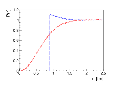
The strong repulsive character of the nucleon-nucleon (NN) interaction at short distances, together with the Pauli exclusion principle, generate short range correlations. In this section, we model these with a hard sphere repulsion or a smoother Gaussian repulsion which mimics the distributions of Ref. Alvioli:2009ab .

A natural measure of the correlation is the ratio between the normalized two-body probability distribution of nucleons and the product of the one-body distributions $f^{(2)}({\boldsymbol{x}}_{1},{\boldsymbol{x}}_{2})/f^{(1)}({\boldsymbol{x}}_{1})f^{(1)}({\boldsymbol{x}}_{2})$ (see Appendix A). In order to see how it varies as a function of the relative distance $r=|{\boldsymbol{x}}_{1}-{\boldsymbol{x}}_{2}|$, we integrate both the numerator and denominator over the mean point:

$$P(r)\equiv\frac{\int{d}^{3}{\boldsymbol{R}}\,f^{(2)}({\boldsymbol{R}}+\frac{{\boldsymbol{r}}}{2},{\boldsymbol{R}}-\frac{{\boldsymbol{r}}}{2})}{\int{d}^{3}{\boldsymbol{R}}\,f^{(1)}({\boldsymbol{R}}+\frac{{\boldsymbol{r}}}{2})f^{(1)}({\boldsymbol{R}}-\frac{{\boldsymbol{r}}}{2})}$$ (18)

The half-integrated pair correlation function $P(r)$ thus defined is plotted in Fig. 1 for the hard sphere and the Gaussian repulsion. Note the strong repulsion dip near the origin, compensated by a slight overshoot above unity at large distances.

Figure 2: (Color online) Same as Fig. 1 but for the distribution in the transverse distance, $P(\rho)$ ($\rho=s$).

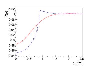
The relevant quantity for the present study, however, is the pair correlation function in the relative transverse distance, obtained by integrating both the numerator and the denominator of Eq. (18) along the collision axis $z$ (in the same way as the nuclear thickness function Miller:2007ri ). The resulting pair correlation function $P(s)$ is shown in Fig. 2. We note that the projection leading from $P(r)$ to $P(s)$ greatly reduces the repulsion dip, from $1$ to $\lesssim 0.15$. This is easy to understand, since the two nucleons may lie close to each other in the transverse plane, i.e., be at small $s$, while being sufficiently separated in $z$, and hence outside the volume over which they feel the short range correlation. This property will allow us to treat these correlations as a small perturbation.

We thus write $P(s)=1-d(s)$, where $d(s)\ll 1$. In the following sections, we use the Gaussian parametrization of the nuclear repulsion, which is more realistic than the hard-sphere repulsion Rybczynski:2011wv . The resulting $d(s)$ is itself Gaussian to a good approximation:

$$d(s)=B\exp\left(-\frac{s^{2}}{2\sigma_{d}^{2}}\right),$$ (19)

$$B=0.11,\;\;\sigma_{d}=0.56~{}{\rm fm},$$

where the numerical values have been fitted to the results shown in Fig. 2. When comparing the cases of nuclear distributions with and without the NN correlations, we make sure that the single-particle distributions $f^{(1)}({\boldsymbol{x}})$ are identical. The way to accomplish this in Monte Carlo studies with NN expulsion distance is explained in Ref. Broniowski:2007nz .

IV Proton-nucleus collisions

In this section, we study the one-body density and the density-density correlation in the proton-nucleus collisions analytically and numerically. We then evaluate fluctuation observables.

We consider central proton-nucleus collisions ($b=0$). We denote with $\theta(s)$ the wounding profile, i.e., the probability that the proton interacts inelastically with a nucleon sitting at a transverse distance $s$ away from it. We use the following Gaussian parametrization Alvioli:2009ab

$$\theta(s)=A\exp\left(-\frac{s^{2}}{2\sigma_{w}^{2}}\right),$$ (20)

$$A=0.92,\;\;\sigma_{w}=1.08~{}{\rm fm}.$$

The normalization reproduces the total inelastic NN cross section, i.e., $\int{d}s\,\theta(s)=2\pi A\sigma_{w}^{2}=\sigma_{NN}^{\rm inel}$. The choice of parameters in Eq. (20) is such that $\sigma_{NN}^{\rm inel}\simeq 68$ mb, corresponding to the LHC energy $\sqrt{s_{NN}}=5.02$ TeV. Nucleons hit by the proton as it crosses the nucleus are referred to as participants or wounded nucleons.

In the model considered here Bzdak:2013zma , a source is produced at mid-distance between the proton and each participant nucleon. Since the proton is by assumption located at the origin, the sources are placed at the positions ${\boldsymbol{z}}_{i}\equiv{\boldsymbol{s}}_{i}/2$, where ${\boldsymbol{s}}_{i}$ denotes the transverse location of the $i^{\rm th}$ participant. Thus there is a one-to-one correspondence between sources and hit nucleons in the target, and all the sources play symmetric roles. Another option is to assume that the sources are created on top of each participant. The resulting differences are discussed briefly at the end of Sec. IV.1.

IV.1 Analytic model

As seen above, the distribution of sources closely follows that of the participants within the target nucleus; in particular, this distribution directly reflects nuclear correlations that are inherited from those among the nucleons of the target nucleus. As explained in Appendix E, for weak correlations, the two-body distribution of the sources is approximately given by (with ${\boldsymbol{s}}_{i}=2{\boldsymbol{z}}_{i}$)

$$f^{(2)}({\boldsymbol{z}}_{1},{\boldsymbol{z}}_{2})\simeq c_{2}\,{\theta({\boldsymbol{s}}_{1})\theta({\boldsymbol{s}}_{2})(1-d(|{\boldsymbol{s}}_{1}-{\boldsymbol{s}}_{2}|))},$$ (21)

where $c_{2}$ is a normalization constant. It is thus entirely determined by the wounding profile $\theta$ and the correlation factor $1-d$.

The one-body distribution $f^{(1)}({\boldsymbol{z}}_{1})$ is obtained by integrating Eq. (21) over ${\boldsymbol{z}}_{2}$ (see Eq. (48)). For uncorrelated nucleons ($d(|{\boldsymbol{s}}_{1}-{\boldsymbol{s}}_{2}|)=0$), it reduces to

$$f^{(1)}({\boldsymbol{z}}_{1})=\frac{1}{n}\langle\rho({\boldsymbol{z}}_{1})\rangle\propto\theta({\boldsymbol{s}}_{1}).$$ (22)

The one-body distribution thus reproduces the wounding profile (20). When the nucleon-nucleon correlations are taken into account, the one-body distribution of the sources changes slightly, even though the one-body distribution of nucleons is strictly unchanged (see the statement at the very end of Sec. III). However, this is a very tiny change in practice, such that Eq. (22) holds to a very good approximation with realistic correlations.

Figure 3: (Color online) The half-integrated pair distribution function $g(\Delta_{x},\Delta_{y})$ for the fireball created in the p+Pb collisions at the impact parameter $b=0$ and the number of participants $n=15$, $\Delta$ is the relative transverse distance between the two sources.

Figure 4: (Color online) Functions $R(\Delta)$ (a) and $g(\Delta)$ (b) defined in Eq. (25) for p+Pb collisions at the impact parameter $b=0$ and the number of participants $n=15$, obtained with GLISSANDO.

In order to study how the density-density correlation depends on the relative distance, we introduce the half-integrated density-density correlation function, much in the same way as in Eq. (18):

$$S({\boldsymbol{\Delta}})=\int{d}{\boldsymbol{r}}\,S({\boldsymbol{r}}+\frac{{\boldsymbol{\Delta}}}{2},{\boldsymbol{r}}-\frac{{\boldsymbol{\Delta}}}{2}).$$ (23)

The decomposition (5) can be easily transposed to the half-integrated correlation:

$$S({\boldsymbol{\Delta}})=\langle n\rangle\delta({\boldsymbol{\Delta}})+R({\boldsymbol{\Delta}})[g({\boldsymbol{\Delta}})-1],$$ (24)

where

$$R({\boldsymbol{\Delta}}) \equiv \int{d}{\boldsymbol{r}}\,\left\langle\rho({\boldsymbol{r}}+\frac{{\boldsymbol{\Delta}}}{2})\right\rangle\left\langle\rho\left({\boldsymbol{r}}-\frac{{\boldsymbol{\Delta}}}{2}\right)\right\rangle,$$ (25)

$$g({\boldsymbol{\Delta}}) \equiv \frac{1}{R({\boldsymbol{\Delta}})}\int{d}{\boldsymbol{r}}\,\left\langle n(n-1)f^{(2)}({\boldsymbol{r}}+\frac{{\boldsymbol{\Delta}}}{2},{\boldsymbol{r}}-\frac{{\boldsymbol{\Delta}}}{2})\right\rangle$$

. (26)

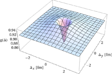
With the approximation of Eq. (21) for the two-body distribution, all integrals can be evaluated analytically. The pair distribution function $g({\boldsymbol{\Delta}})$ is plotted in Fig. 3 (right). The central dip reflects the short-range nucleon-nucleon repulsion. As a crude approximation, by using Eq. (22), one may replace $\theta({\boldsymbol{s}}_{i})$ by $f^{1}({\boldsymbol{z}}_{i})$ in Eq. (21), and write $f^{(2)}({\boldsymbol{z}}_{1},{\boldsymbol{z}}_{2})\simeq f^{(1)}({\boldsymbol{z}}_{1})f^{(1)}({\boldsymbol{z}}_{2})(1-d(|{\boldsymbol{s}}_{1}-{\boldsymbol{s}}_{2}|))$. One thus obtains

$$g({\boldsymbol{\Delta}})\simeq\left(1-\frac{1}{n}\right)(1-d(2\Delta)),$$ (27)

where we have used the fact that the source is half-way between the nucleons, ${\boldsymbol{s}}_{i}=2{\boldsymbol{z}}_{i}$. Eq. (27) is a good approximation to the exact result in Fig. 3. A more careful calculation, enforcing the proper normalization, shows that this approximation only holds when the range of correlations is much smaller than the wounding profile, $\sigma_{d}\ll\sigma_{w}$, a condition which is only marginally satisfied with the chosen numerical values.

The simplicity of the results in Eqs. (22) and (27) is a consequence of the prescription to locate sources half-way between the proton and the wounded nucleons. If one chooses instead the “standard” prescription where sources are located around each participant, the proton also acts as a source in addition to the hit nucleons: this results in cumbersome expressions for the one-body and two-body densities, but no new insight.

IV.2 Monte Carlo simulations

We now show that our simple analytic results, based on the approximation of weak correlations, are fully supported by numerical simulations made with GLISSANDO Broniowski:2007nz at zero impact parameter, $b=0$. The condition $b=0$ is not realistic, in the sense that it cannot be implemented experimentally. On the other hand, it allows us to clearly isolate correlations which do not originate in impact parameter fluctuations. For sake of simplicity, we fix the number of participants to $n=15$, corresponding to a typical value at the LHC energy. In the presented simulations we are using the correlated nuclear distributions of Ref. Alvioli:2009ab and the Gaussian wounding profile Rybczynski:2011wv of Eq. (20).

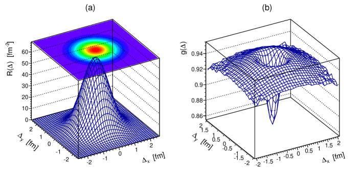
In Fig. 4 we show the two-dimensional plots of the simulated half-integrated correlation function $R(\Delta)$, and the pair correlation function $g(\Delta)$ of Eq. (25). The function $R(\Delta)$ simply reflects the shape of the folding of the two single-particle distributions, while $g(\Delta)$ is remarkably close to the result of the analytic calculation presented in Fig. 3.

IV.3 Observables

The approximations made in Sec. IV.1 (specifically, Eqs.(19), (20) and (21)) allow us to obtain analytic expressions of observables introduced in Sec. II.3. For a fixed number of participants $n$, the mean squared radius, Eq. (8), is

$$\langle r_{\rm rms}^{2}\rangle = \int{d}^{2}{\boldsymbol{x}}\,r^{2}f^{(1)}({\boldsymbol{x}})$$ (28)

$$= \frac{\sigma_{w}^{2}}{2}\left(1+B\frac{\sigma_{d}^{2}\sigma_{w}^{2}}{\left(\sigma_{d}^{2}+2\sigma_{w}^{2}\right)^{2}}+{\cal O}\left(B^{2}\right)\right),$$ (29)

where the one-body density $f^{(1)}({\boldsymbol{x}})$ has been obtained by integrating Eq. (21). If nucleons are uncorrelated ($B=0$), the rms radius is proportional to the wounding radius $\sigma_{w}$. The proportionality constant would be typically a factor 2 larger if we had assumed that the sources were on top of the participants, instead of half-way between the proton and the participants in the target nucleus.

Equation (28) shows that repulsive correlations ($B>0$) result in a very small increase of the fireball size. The effect of correlations vanishes not only in the limit of a small correlation length, $\sigma_{d}\ll\sigma_{w}$, but also in the opposite limit where the correlation length is much larger than the fireball size, $\sigma_{d}\gg\sigma_{w}$. This is a general result, as we shall see below for other observables. Numerically, the increase of $\langle r_{\rm rms}^{2}\rangle$ due to repulsive correlations is a modest $0.6$%.

We now evaluate fluctuation observables, namely, the variance of the mean-square radius and the mean square eccentricity. In the uncorrelated case ($B=0$), Eq. (15) simplifies to

$${\rm Var}(r_{\rm rms}^{2})^{\rm no~{}corr.} = \frac{\langle r_{\rm rms}^{2}\rangle^{2}}{n},$$ (30)

$${\rm Var}(\varepsilon_{2})^{\rm no~{}corr.} = \frac{2}{n},$$ (31)

where we have used the fact that the one-body distribution, Eq. (22), is Gaussian.

We finally evaluate the changes in these observables due to correlations ($B>0$), which are conveniently expressed by the ratio of Eq. (17). Correlations modify all terms in the density-density correlation function Eq. (5): The autocorrelation term changes slightly due to the modification of the one-body distribution of sources. We neglect this contribution, which is typically less than 1%, and evaluate the contribution of pair correlations. This contribution is enhanced by a factor $n$ because the pair correlation $g({\boldsymbol{x}},{\boldsymbol{y}})$ in Eq. (5) is multiplied by a the square of the average density, which scales as $n^{2}$, while the autocorrelation term only scales as $n$. After some algebra, one obtains

$$R(r_{\rm rms}^{2}) = 1-2nB\frac{\sigma_{d}^{2}\sigma_{w}^{4}}{\left(\sigma_{d}^{2}+2\sigma_{w}^{2}\right)^{3}}+{\cal O}\left(B^{2}\right),$$ (32)

$$R(\varepsilon_{2}) = 1-nB\frac{\sigma_{d}^{2}\sigma_{w}^{4}}{\left(\sigma_{d}^{2}+2\sigma_{w}^{2}\right)^{3}}+{\cal O}\left(B^{2}\right).$$ (33)

Numerically, correlations decrease $\langle|\varepsilon_{2}|^{2}\rangle$ by a modest 4%. We have also evaluated numerically their effect of $\langle|\varepsilon_{3}|^{2}\rangle$ which is even smaller, at the level of 1%. Generally, effects of correlations are usually even smaller when realistic NN correlations are implemented Alvioli:2011sk , rather than just the short-range part considered here. We conclude that for the proton-nucleus collisions in the Glauber model, correlations between sources are essentially negligible for the considered observables.

V Nucleus-nucleus collisions

The Glauber Czyz:1969jg ; Bialas:1976ed ; Bialas:2008zza description of the A+A collisions is inherently more complicated than that of the p+A collisions. We are no longer able to determine analytically the distribution of sources, and hence deduce their correlations with analytic tools. Nevertheless, one can get a simple understanding of these correlations in the two limiting cases of small and large inelastic cross sections. Further understanding is gained through GLISSANDO simulations.

V.1 Twin correlations

In the wounded-nucleon model, the density is created by participant nucleons, which come from one of the two colliding nuclei $A$ and $B$. By definition, to each participant in nucleus $A$ corresponds at least one participant in nucleus $B$, at a distance of the order $\sqrt{\sigma_{NN}^{\rm inel}}$ in the transverse plane. This condition creates nontrivial correlations between participants, which we dub “twin” correlations. The effect of the twin correlations can be easily understood in the limits of very small or very large wounding cross section $\sigma_{NN}^{\rm inel}$.

For this discussion, it is useful to separate the contributions of the sources coming from nuclei $A$ and $B$, respectively, and write the total density of sources as $\rho({\boldsymbol{x}})=\rho_{A}({\boldsymbol{x}})+\rho_{B}({\boldsymbol{x}})$. In the limit of small $\sigma_{NN}^{\rm inel}$, each nucleon of $A$ sees at most one nucleon of $B$, i.e., the wounded nucleons come in pairs, one from nucleus $A$ and the other one from nucleus $B$. Furthermore, the smallness of the cross section also implies that both nucleons in the pair are close to each other in the transverse plane. Thus, if there is a source from nucleus $A$ at point ${\boldsymbol{x}}$, there is also a source from nucleus $B$ at the almost same point ${\boldsymbol{x}}$, therefore $\rho_{A}({\boldsymbol{x}})\simeq\rho_{B}({\boldsymbol{x}})$. One can take into account the correlations among sources within nucleus $A$ by defining a density-density correlation $S_{A}({\boldsymbol{x}},{\boldsymbol{y}})$, and decomposing it according to Eq. (5):

$$S_{A}({\boldsymbol{x}},{\boldsymbol{y}}) = \langle\rho_{A}({\boldsymbol{x}})\rangle\delta({\boldsymbol{x}}-{\boldsymbol{y}})$$ (35)

$$+\langle\rho_{A}({\boldsymbol{x}})\rangle\langle\rho_{A}({\boldsymbol{y}})\rangle[g_{A}({\boldsymbol{x}},{\boldsymbol{y}})-1].$$

Since $\rho({\boldsymbol{x}})\simeq 2\rho_{A}({\boldsymbol{x}})$, the full density-density correlation function is $S({\boldsymbol{x}},{\boldsymbol{y}})\simeq 4S_{A}({\boldsymbol{x}},{\boldsymbol{y}})$, and the previous equation gives

$$S({\boldsymbol{x}},{\boldsymbol{y}}) = 2\langle\rho({\boldsymbol{x}})\rangle\delta({\boldsymbol{x}}-{\boldsymbol{y}})$$ (37)

$$+\langle\rho({\boldsymbol{x}})\rangle\langle\rho({\boldsymbol{y}})\rangle[g_{A}({\boldsymbol{x}},{\boldsymbol{y}})-1].$$

Comparing with the general decomposition (5), one sees that the twin correlations double the autocorrelation term. Equivalently, they give a $\delta$ contribution to the pair distribution function:

$$g({\boldsymbol{x}},{\boldsymbol{y}})=g_{A}({\boldsymbol{x}},{\boldsymbol{y}})+\frac{1}{\langle\rho({\boldsymbol{y}})\rangle}\delta({\boldsymbol{x}}-{\boldsymbol{y}}).$$ (38)

Figure 5: (Color online) The half-integrated pair correlation function $g(\Delta)$ for Pb-Pb collisions at impact parameter $b=0$ with $\sigma_{NN}^{\rm inel}=20$ mb and $n=371$. No NN repulsion in the nuclear distributions is included. A sharp peak from the twin-production mechanism is clearly visible.

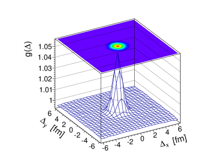
Fig. 5 illustrates this result with a Monte Carlo Glauber simulation carried out for central ($b=0$) Pb-Pb collisions with a value of the cross section much lower than the actual value at the LHC, namely, $\sigma_{NN}^{\rm inel}=20$ mb. We use a Gaussian wounding profile. In order to eliminate effects of multiplicity fluctuations, we select events with a fixed number of wounded nucleons $n$, corresponding to the most probable value for this choice of $\sigma_{NN}^{\rm inel}$ (this value is obtained by first running a minimum-bias calculation and then choosing the most frequent value of $n$). In order to isolate the effect of the twin correlations, we switch off the nuclear correlations studied in Sec. III as well as the correlations from recentering (cf. Appendix D): as a consequence, $g_{A}({\boldsymbol{x}},{\boldsymbol{y}})$ in Eq. (38) is a constant (see Eq. (6)). The half-integrated pair distribution function $g(\Delta)$, with $\Delta={\boldsymbol{x}}-{\boldsymbol{y}}$, clearly shows the sharp positive peak expected from Eq. (38). The finite width corresponds to the finite value of $\sigma_{NN}^{\rm inel}$. Note that the asymptotic value at large relative distance $\Delta$, where correlations are negligible, is slightly smaller than unity, and approximately given by Eq. (6).

Figure 6: (Color online) Same as Fig. 5 but for with $\sigma_{NN}^{\rm inel}=68$ mb and $n=410$ (i.e., we again fix $n$ to its most probable value). We observe a significant melting of the peak compared to Fig. 5.

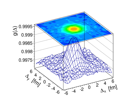
Fig. 6 illustrates the effect of increasing the cross section up to the actual value at the LHC, $\sigma_{NN}^{\rm inel}=68$ mb. Naturally, the width of the correlation peak increases proportionally to $\sqrt{\sigma_{NN}^{\rm inel}}$. Meanwhile, the height of the peak decreases by a factor $\sim 35$, such that the integral of the peak decreases by a factor $\sim 10$. We have checked that as one further increases $\sigma_{NN}^{\rm inel}$, the peak broadens and completely melts down: The twin correlations disappear. This can also be easily understood: In the limit of infinite $\sigma_{NN}^{\rm inel}$, all the nucleons are wounded, hence become uncorrelated.

The dimensionless control parameter separating the regimes of “small” and “large” wounding cross section is the average number of target nucleons hit by each projectile nucleon, which we denote by $\cal N$: this is roughly the product of the average density $A/(\pi R_{A}^{2})$ with $R_{A}$, the nuclear radius, and the cross section $\sigma_{NN}^{\rm inel}$. Taking $R_{A}\simeq A^{1/3}r_{0}$, with $r_{0}=1.2$ fm, one obtains

$${\cal N}\sim\frac{A^{1/3}\sigma_{NN}^{\rm inel}}{\pi r_{0}^{2}}\simeq 4\frac{\sigma_{NN}^{\rm inel}[{\rm fm}^{2}]}{\pi},$$ (39)

where, in the last equality, we have chosen $A=208$. The value $\sigma_{NN}^{\rm inel}=20$ mb chosen in Fig. 5 corresponds to ${\cal N}\sim 2.6$, a number significantly larger than unity: The twin correlations are already significantly suppressed for this value of the cross section, which explains why the peak is only a few percent above unity.

The strength of the twin correlations can also be investigated differentially as a function of the position in the transverse plane. For realistic values of $\sigma_{NN}^{\rm inel}$, all nucleons in the center are wounded, and the twin correlations are only present near the boundary of the fireball. This expectation is confirmed by our numerical simulations.

Finally, if one takes into account repulsive nuclear correlations (Sec. III), the correlation functions of Figs. 5 and 6 display an additional central dip, as in Fig. 4 (b), thus partially hiding the effect of the twin correlations.

V.2 Fluctuation observables

Figure 7: (Color online) The ratios defined in Eq. (17) for the Pb+Pb collisions at various values of the total inelastic NN cross section, $\sigma_{NN}^{\rm inel}$. The corresponding fixed values of the number of the wounded nucleons, $n$, is shown on the upper horizontal axis.

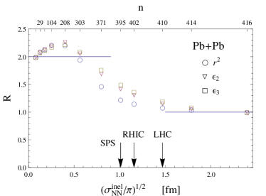
We now study numerically the effect of the twin correlations on fluctuation observables, namely, the variances of $r_{\rm rms}^{2}$, $\varepsilon_{2}$, $\varepsilon_{3}$. To this end, we evaluate for each observable the ratio $R$ in Eq. (17), which gives its relative increase due to correlations. These ratios are plotted in Fig. 7 as a function of $\sigma_{NN}^{\rm inel}$. As in Sec. V.1, we simulate central Pb-Pb collisions, where nuclear correlations are switched off, and we fix the number of wounded nucleons $n$ to its most probable value for each value of of $\sigma_{NN}^{\rm inel}$. The limits $\sigma_{NN}^{\rm inel}\to 0$ and $\sigma_{NN}^{\rm inel}\to\infty$ are readily understood from the discussion of Sec. V.1. For small $\sigma_{NN}^{\rm inel}$, the twin correlations double the density-density correlation with respect to the uncorrelated case, hence all ratios tend to 2. For large $\sigma_{NN}^{\rm inel}$, the twin correlations vanish and all ratios approach 1. The behavior between these two limits controlled by the parameter ${\cal N}$ in Eq. (39), which is 1 for $(\sigma_{NN}^{\rm inel}/\pi)^{1/2}\simeq 0.5$. This behavior is nontrivial: in particular, all ratios increase above 2 before deceasing to 1. This increase is an effect of induced secondary correlations: a nucleon from nucleus $A$ wounds a nucleon from nucleus $B$, which in turn wounds another nucleon from nucleus $A$, thus inducing a correlation between participants of nucleus $A$. Note that while all three curves have the same asymptotic limits, intermediate values differ depending on the observable. At the values of the wounding cross section corresponding to the collisions at RHIC and the LHC (42 mb, and 68 mb, respectively), the ratios are closer to the uncorrelated limit.

Our result at the RHIC energy is somewhat smaller than that of Alver et al. Alver:2008zza , where the ratios of physical to mixed-event results were presented. However, their calculation is slightly different: in particular, they do not fix the impact parameter or the number of participants, thus including more sources of fluctuations which increase the variance. Similarly, it was found in Ref. Bhalerao:2011bp that correlations increase the variance of $\varepsilon_{2}$ and $\varepsilon_{3}$ by a factor $\sim 2$ at RHIC and the LHC. The difference with our result is likely due to the fact that the present simulation gives an identical weight to each wounded nucleon, in contrast with the usual implementation at RHIC or the LHC where weights increase linearly with the number of binary collisions Miller:2007ri . Generally, one expects that any additional source of fluctuations Alvioli:2013vk ; Rybczynski:2013mla will increase the variance, thus producing an effect similar to the twin correlations.

Figure 8: (Color online) Same as Fig. 7 but for the case where wounded nucleons coming only from one nucleus are taken into account.

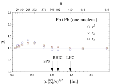
In order to further investigate the origin of correlations, in particular confirm the mechanism of secondary correlations, we now repeat the simulation using a modified Glauber model, where participants from only one nucleus contribute to the density. In other terms, we assume $\rho({\boldsymbol{x}})=\rho_{A}({\boldsymbol{x}})$, following the notations of Sec. V.1. In the wounded nucleon model, this corresponds to the density at very forward rapidity Bozek:2010vz . This modification effectively switches off direct twin correlations, which involve nucleons from different nuclei. The resulting values of $R$ are displayed in Fig. 8. Correlations now disappear in both limits of large and small $\sigma_{NN}^{\rm inel}$, as expected. The departure from unity at intermediate values of $\sigma_{NN}^{\rm inel}$ is again an effect of induced secondary correlations. We note that at the SPS, RHIC, and LHC energies, the secondary correlations are negligible.

Figure 9: (Color online) Same as Fig. 7 but for the case where nuclear distributions of Ref. Alvioli:2009ab with NN repulsion are used.

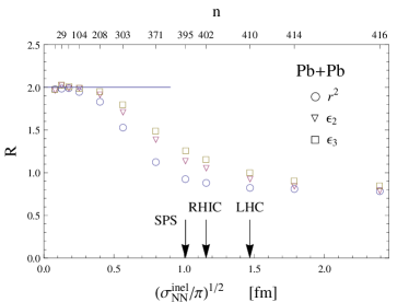
Finally, we study the combined effects of the twin correlations and nuclear correlations Alvioli:2009ab . Results are presented in Fig. 9. As already shown in Ref. Broniowski:2010jd , repulsive correlations result in a sizable decrease of fluctuation observables, which is at the level of 20% for large $\sigma_{NN}^{\rm inel}$. Let us analyze the origin of this result. Much of the discussion of Sec. IV.1 can be carried over to the nucleus-nucleus collisions. For large $\sigma_{NN}^{\rm inel}$, the twin correlations are negligible, and the only correlations among sources are those already present in the colliding nuclei. We therefore write

$$f^{(2)}({\boldsymbol{x}},{\boldsymbol{y}})\simeq f^{(1)}({\boldsymbol{x}})f^{(1)}({\boldsymbol{y}})\left(1-\frac{1}{2}d(|{\boldsymbol{x}}-{\boldsymbol{y}}|)\right),$$ (40)

where the factor $1/2$ accounts for the fact that only pairs of sources from the same nucleus are correlated (neglecting $1/n$ corrections). In writing Eq. (40), we neglect the small change of normalization induced by the repulsive correlation, i.e., we assume

$$\int{d}^{2}{\boldsymbol{x}}{d}^{2}{\boldsymbol{y}}f^{(1)}({\boldsymbol{x}})f^{(1)}({\boldsymbol{y}})d(|{\boldsymbol{x}}-{\boldsymbol{y}}|)\ll 1.$$ (41)

Inserting Eq. (40) into Eq. (56), and ignoring small corrections of order $1/n$, one obtains

$$g({\boldsymbol{x}},{\boldsymbol{y}})\simeq 1-\frac{1}{2}d(|{\boldsymbol{x}}-{\boldsymbol{y}}|).$$ (42)

Inserting this equation into Eq. (5) yields

$$S({\boldsymbol{x}},{\boldsymbol{y}}) \simeq \langle\rho({\boldsymbol{x}})\rangle\delta({\boldsymbol{x}}-{\boldsymbol{y}})-\frac{1}{2}\langle\rho({\boldsymbol{x}})\rangle\langle\rho({\boldsymbol{y}})\rangle d({\boldsymbol{x}}-{\boldsymbol{y}})$$ (43)

$$\simeq \langle\rho({\boldsymbol{x}})\rangle\delta({\boldsymbol{x}}-{\boldsymbol{y}})-\frac{1}{2}\langle\rho({\boldsymbol{x}})\rangle^{2}d({\boldsymbol{x}}-{\boldsymbol{y}}),$$ (44)

where in the second line we have used the fact that the range of the nucleon-nucleon correlation is much shorter than the nuclear radius, such that $\rho({\boldsymbol{x}})\simeq\rho({\boldsymbol{y}})$. Note that Eq. (43) does not satisfy the normalization condition Eq. (4): the integral of $S({\boldsymbol{x}},{\boldsymbol{y}})$ should be 0. A more careful calculation (enforcing the proper normalization in Eq. (40) and restoring terms of order $1/n$ in Eq. (42)) shows that $S({\boldsymbol{x}},{\boldsymbol{y}})$ has an additional disconnected term of the form $c\langle\rho({\boldsymbol{x}})\rangle\langle\rho({\boldsymbol{y}})\rangle$. This disconnected term, however, does not contribute to the $\varepsilon_{n}$ fluctuations for symmetry reasons, as already noted at the end of Sec. II.3.

Inserting Eq. (43) into Eqs. (13) and (17) results in

$$R(\varepsilon_{l}) = 1-\frac{1}{2}\frac{\int\langle\rho({\boldsymbol{x}})\rangle^{2}r^{2l}{d}^{2}{\boldsymbol{x}}}{\int\langle\rho({\boldsymbol{x}})\rangle r^{2l}{d}^{2}{\boldsymbol{x}}}\int d(s){d}^{2}{\boldsymbol{s}}.$$ (45)

To get numerical estimates we take a rough approximation where $\langle\rho({\boldsymbol{x}})\rangle$ is a projection of a uniform sphere of radius $R_{A}$ on a plane, $\langle\rho({\boldsymbol{x}})\rangle=6n\sqrt{R_{A}^{2}-x^{2}}/(4\pi R_{A}^{3})$. Then

$$R(\varepsilon_{l}) \sim 1-\frac{3nB\sigma_{d}^{2}\Gamma(l+5/2)}{\sqrt{\pi}R_{A}^{2}\Gamma(l+3)},$$ (46)

which yields for $n=416$ the values $R(\varepsilon_{2})\sim 0.71$ and $R(\varepsilon_{3})\sim 0.74$, in approximate agreement (at the level of 10%) with the detailed simulation shown in Fig. 9.

As in the case of the proton-nucleus collisions (Eq. (32)), the effect of nuclear correlations is enhanced by a factor $n$. Our results show that a repulsive short-range correlation always reduces the $\varepsilon_{n}$ fluctuations. It has been found numerically Alvioli:2011sk that when realistic two- and three-body correlations are implemented, the rms anisotropy barely changes, which suggests that the short-range repulsive NN correlation is compensated by a intermediate-range attractive NN correlation.

VI Conclusions

We have shown that quantities characterizing fluctuations in the early phase of relativistic heavy-ion and proton-nucleus collisions — specifically, the size and eccentricity fluctuations — can be generally expressed in terms of the density-density correlation. We have analyzed the structure of this density-density correlation within the Monte Carlo Glauber model. It can be written as the sum of an autocorrelation part, which is the contribution of fluctuations, and a part involving genuine two-body correlations.

We have investigated in detail the effect of these genuine correlations on selected observables. We have shown that effects of the nucleon-nucleon correlations inside colliding nuclei are parametrically enhanced by a factor $n$, where $n$ is the number of participants, yet they are expected to be small with realistic interactions Alvioli:2011sk . For nucleus-nucleus collisions, we have identified a new type of correlations, due to the collision mechanism itself, which we have dubbed twin correlations; they increase fluctuations. At the RHIC and LHC energies, however, the nucleon-nucleon cross section is so large that essentially all nucleons in the interaction region are wounded. As a result, the twin correlations are small and localized near the boundary of the fireball.

All sources of correlations studied in this paper — namely, the autocorrelation, nuclear correlations, and the twin correlations — involve scales much shorter than the nuclear radius. The eccentricity and size fluctuations in the Glauber model appear then to be created by uncorrelated, small-scale fluctuations in the transverse plane. Subnucleonic fluctuations, which are not incorporated in the Glauber model, are also intrinsically small-scale phenomena. They typically increase the magnitude of the local fluctuations, but do not give rise to any large-distance correlation. To a good approximation, the Monte-Carlo Glauber model provides a picture of energy deposition for the RHIC at LHC energies in terms of independent sources, that seems to capture the main features of these fluctuations and their correlations.

Appendix A Distributions of sources

The sources are defined by their locations $\{{\boldsymbol{x}}_{i}\}$ in the transverse plane and by their number $n$. The positions $\{{\boldsymbol{x}}_{i}\}$ and the number $n$ are random variables that fluctuate from event to event. For a given $n$, we denote by $f_{n}({\boldsymbol{x}}_{1},...,{\boldsymbol{x}}_{n})$ the probability distribution that sources are localized at ${\boldsymbol{x}}_{1},...,{\boldsymbol{x}}_{n}$. By definition, $f_{n}$ is completely symmetric. The $k$-body distribution is defined by integrating over $n-k$ positions:

$$f_{n}^{(k)}({\boldsymbol{x}}_{1},..,{\boldsymbol{x}}_{k})=\int{d}^{2}{\boldsymbol{x}}_{k+1}...{d}^{2}{\boldsymbol{x}}_{n}\,f_{n}({\boldsymbol{x}}_{1},...,{\boldsymbol{x}}_{n}).$$ (47)

In particular, the one-body density can be obtained by integrating the 2-body density:

$$f_{n}^{(1)}({\boldsymbol{x}}_{1})=\int{d}^{2}{\boldsymbol{x}}_{2}\,f_{n}^{(2)}({\boldsymbol{x}}_{1},{\boldsymbol{x}}_{2}).$$ (48)

Note that in general the $k$-body distribution thus defined depends on the total number of sources $n$. Note also that $\int{d}^{2}x\,f_{n}^{(1)}({\boldsymbol{x}})=1$.

The average value of the density $\rho({\boldsymbol{x}})$ (Eq.(1)) is

$$\langle\rho({\boldsymbol{x}})\rangle = \langle\int{d}^{2}{\boldsymbol{x}}_{1}...{d}^{2}{\boldsymbol{x}}_{n}\,f_{n}({\boldsymbol{x}}_{1},...,{\boldsymbol{x}}_{n})\sum_{i=1}^{n}\delta({\boldsymbol{x}}-{\boldsymbol{x}}_{i})\rangle$$ (49)

$$= \langle nf_{n}^{(1)}({\boldsymbol{x}})\rangle,$$ (50)

where we have allowed the multiplicity $n$ to fluctuate for sake of generality, and the angular brackets in the right-hand side of Eq. (50) denote an average over the distribution of $n$. Similarly,

$$\langle\rho({\boldsymbol{x}})\rho({\boldsymbol{y}})\rangle=$$

$$\langle\int{d}^{2}{\boldsymbol{x}}_{1}...{d}^{2}{\boldsymbol{x}}_{n}\,f_{n}({\boldsymbol{x}}_{1},...,{\boldsymbol{x}}_{n})\sum_{i,j}\delta({\boldsymbol{x}}\!-\!{\boldsymbol{x}}_{i})\delta({\boldsymbol{y}}\!-\!{\boldsymbol{x}}_{j})\rangle$$

$$=\langle nf_{n}^{(1)}({\boldsymbol{x}})\rangle\delta({\boldsymbol{x}}-{\boldsymbol{y}})+\langle n(n-1)f_{n}^{(2)}({\boldsymbol{x}},{\boldsymbol{y}})\rangle.$$ (51)

Equations (50,51) yield the following generic decomposition of the density-density correlation function (3):

$$S({\boldsymbol{x}},{\boldsymbol{y}}) = \langle nf_{n}^{(1)}({\boldsymbol{x}})\rangle\delta({\boldsymbol{x}}-{\boldsymbol{y}})$$

$$+ \langle n(n-1)f_{n}^{(2)}({\boldsymbol{x}},{\boldsymbol{y}})\rangle-\langle nf_{n}^{(1)}({\boldsymbol{x}})\rangle\langle nf_{n}^{(1)}({\boldsymbol{y}})\rangle.$$

The first term is commonly referred to as an autocorrelation, the second term is the inclusive distribution of pairs, and the last term is the disconnected part, composed of the product of the inclusive single-particle distributions. Note that the autocorrelation term follows from the rearrangement of the sums in the definition Eq. (51). It represents a major contribution to the correlation function and is by all means physical. Using Eq. (50), one can rewrite Eq. (A) as

$$S({\boldsymbol{x}},{\boldsymbol{y}}) = \langle\rho({\boldsymbol{x}})\rangle\delta({\boldsymbol{x}}-{\boldsymbol{y}})$$ (53)

$$+ \langle n(n-1)f_{n}^{(2)}({\boldsymbol{x}},{\boldsymbol{y}})\rangle-\langle\rho({\boldsymbol{x}})\rangle\langle\rho({\boldsymbol{y}})\rangle.$$

The pair distribution function is defined by

$$g({\boldsymbol{x}},{\boldsymbol{y}})=\frac{\langle n(n-1)f_{n}^{(2)}({\boldsymbol{x}},{\boldsymbol{y}})\rangle}{\langle\rho({\boldsymbol{x}})\rangle\langle\rho({\boldsymbol{y}})\rangle}.$$ (54)

Inserting into Eq. (53), one obtains Eq. (5). Occasionally, we also use a differently normalized pair correlation function

$$P({\boldsymbol{x}},{\boldsymbol{y}})=\frac{\langle n\rangle^{2}}{\langle n(n-1)\rangle}g({\boldsymbol{x}},{\boldsymbol{y}}),$$ (55)

which asymptotes to unity in the absence of correlations.

In this paper, we carry out simulations where $n$ is fixed. In this case, one can drop the subscript $n$ and Eq. (54) simplifies to:

$$g({\boldsymbol{x}},{\boldsymbol{y}})=\left(1-\frac{1}{n}\right)\frac{f^{(2)}({\boldsymbol{x}},{\boldsymbol{y}})}{f^{(1)}({\boldsymbol{x}})f^{(1)}({\boldsymbol{y}})}.$$ (56)

When no correlations are present, the $n$-particle distribution function is a product of the single-particle distributions. In particular,

$$f^{(2)}({\boldsymbol{x}},{\boldsymbol{y}})=f^{(1)}({\boldsymbol{x}})f^{(1)}({\boldsymbol{y}}),$$ (57)

and $g({\boldsymbol{x}},{\boldsymbol{y}})$ takes the form displayed in Eq. (6), while $P({\boldsymbol{x}},{\boldsymbol{y}})=1$.

Appendix B Superposition models

In Eq. (1), we assume that the strength of each source is the same. This restriction is lifted in superposition models, where the strength of the source is allowed to fluctuate. In this case, one introduces an additional random variable $w_{i}$ that measures the strength of the source $i$, and writes the density $\rho({\boldsymbol{x}})$ as

$$\rho({\boldsymbol{x}})=\sum_{i=1}^{n}w_{i}\delta({\boldsymbol{x}}-{\boldsymbol{x}}_{i}),$$ (58)

with the weights $w_{i}$ generated according to some suitable statistical distribution.

One generally assumes for simplicity that the weight of a source, $w_{i}$, is uncorrelated with its location ${\boldsymbol{x}}_{i}$. One also assumes that weights of different sources are not correlated with one another or with the multiplicity $n$. Then, Eqs. (50) and (5) are replaced respectively by

$$\langle\rho({\boldsymbol{x}})\rangle = \langle w\rangle\langle nf_{n}^{(1)}(x)\rangle,$$ (59)

and

$$S({\boldsymbol{x}},{\boldsymbol{y}}) = \frac{\langle w^{2}\rangle}{\langle w\rangle}\langle\rho({\boldsymbol{x}})\rangle\delta({\boldsymbol{x}}-{\boldsymbol{y}})$$ (60)

$$+ \langle\rho({\boldsymbol{x}})\rangle\langle\rho({\boldsymbol{y}})\rangle[g({\boldsymbol{x}},{\boldsymbol{y}})-1],$$

while the pair distribution function remains given by Eq. (54). Comparison of Eq. (60) with Eq. (5) shows that fluctuations of the weight $w$ enhance the relative contribution of the autocorrelation term.

Appendix C Smearing

In a more realistic situation, the sources may be attributed a finite width. This can be implemented by smearing the point-like source with a finite-width function, $s$: One replaces Eq. (58) by

$$\rho({\boldsymbol{x}})=\sum_{i=1}^{n}w_{i}s({\boldsymbol{x}}-{\boldsymbol{x}}_{i}).$$ (61)

Then, Eqs. (59) and (51) are replaced by

$$\langle\rho({\boldsymbol{x}})\rangle = \langle w\rangle\int{d}^{2}{\boldsymbol{x}}_{1}s({\boldsymbol{x}}-{\boldsymbol{x}}_{1})\langle nf_{n}^{(1)}({\boldsymbol{x}}_{1})\rangle,$$ (62)

and

$$\langle\rho({\boldsymbol{x}})\rho({\boldsymbol{y}})\rangle=$$

$$\langle w^{2}\rangle\int{d}^{2}{\boldsymbol{x}}_{1}s({\boldsymbol{x}}_{1}-{\boldsymbol{x}})s({\boldsymbol{x}}_{1}-{\boldsymbol{y}})\langle nf_{n}^{(1)}({\boldsymbol{x}}_{1})\rangle+$$

$$\langle w\rangle^{2}\int{d}^{2}{\boldsymbol{x}}_{1}{d}^{2}{\boldsymbol{x}}_{2}s({\boldsymbol{x}}_{1}-{\boldsymbol{x}})s({\boldsymbol{x}}_{2}-{\boldsymbol{y}})\langle nf_{n}^{(2)}({\boldsymbol{x}}_{1},{\boldsymbol{x}}_{2})\rangle.$$

Note that the autocorrelation term is no longer singular. A typical choice for the smearing function in practical applications is a Gaussian of a width of a fraction of a fermi Holopainen:2010gz ; Schenke:2010rr ; Bozek:2012gr .

Appendix D Correlations from recentering

For completeness, we also discuss the long-range correlations present in the Monte Carlo simulations due to recentering, i.e., the condition that the center of mass of each nucleus is fixed at a given location in each event. Recentering is implemented in calculating initial anisotropies: they are evaluated in a coordinate system where the fireball is centered Teaney:2010vd .

In each event, the two-dimensional transverse coordinates ${\boldsymbol{x}}_{1},\cdots,{\boldsymbol{x}}_{n}$ are independent. We denote their distribution by $f({\boldsymbol{x}}_{i})$. Without loss of generality we may assume $\langle{\boldsymbol{x}}_{i}\rangle=\int{\boldsymbol{x}}_{i}f({\boldsymbol{x}}_{i}){d}{\boldsymbol{x}}_{i}=0$. The recentered coordinate is defined by

$${\boldsymbol{x}}^{\prime}_{1}={\boldsymbol{x}}_{1}-\frac{{\boldsymbol{x}}_{1}+\cdots+{\boldsymbol{x}}_{n}}{n}=\frac{n-1}{n}\left({\boldsymbol{x}}_{1}-\frac{{\boldsymbol{x}}_{2}+\cdots+{\boldsymbol{x}}_{n}}{n-1}\right)$$

$$=\frac{n-1}{n}\left({\boldsymbol{x}}_{1}-{\boldsymbol{T}}\right),$$ (64)

where we have introduced the auxiliary variable

$${\boldsymbol{T}}\equiv\frac{{\boldsymbol{x}}_{2}+\cdots+{\boldsymbol{x}}_{n}}{n-1}.$$ (65)

In the limit $n\gg 1$, the distribution of ${\boldsymbol{T}}$ is Gaussian according to the central limit theorem. Its normalized distribution is $P_{n-1}({\boldsymbol{T}})$, where

$$P_{k}({\boldsymbol{T}})={\frac{k}{2\pi\sigma^{2}}}\exp\left(-\frac{kT^{2}}{2\sigma^{2}}\right),$$ (66)

with $\sigma^{2}\equiv\langle{\boldsymbol{x}}_{i}^{2}\rangle$ assumed to be identical for all $i$. Furthermore, ${\boldsymbol{x}}_{1}$ and ${\boldsymbol{T}}$ are independent variables, such that the distribution of ${\boldsymbol{x}}^{\prime}_{1}$ as defined in Eq. (D) is

$$f_{n}^{(1)}({\boldsymbol{x}}^{\prime}_{1}) = \int f({\boldsymbol{x}}_{1}){d}^{2}{\boldsymbol{x}}_{1}P_{n-1}({\boldsymbol{T}}){d}^{2}{\boldsymbol{T}}$$

$$\times\delta\left({\boldsymbol{x}}^{\prime}_{1}-\frac{n-1}{n}({\boldsymbol{x}}_{1}-T)\right)$$

$$= \frac{n}{n-1}\int f\left(\frac{n{\boldsymbol{x}}^{\prime}_{1}}{n-1}+{\boldsymbol{T}}\right)P_{n-1}(T){d}^{2}{\boldsymbol{T}}.$$

Then we find easily

$$\langle{\boldsymbol{x}}^{\prime}_{1}\rangle_{s}=\langle{\boldsymbol{x}}_{1}\rangle\;(=0),\;$$

$${\rm Var}_{s}({\boldsymbol{x}}^{\prime}_{1})=\left(1-\frac{1}{n^{2}}\right)\sigma^{2},$$ (70)

Hence the recentered distributions are shrunk by a term of the order $1/n^{2}$.

Carrying out a similar calculation for the case of the two-particle distributions we arrive at

$$f_{n}^{(2)}({\boldsymbol{x}}^{\prime}_{1},{\boldsymbol{x}}^{\prime}_{2}) = \int f({\boldsymbol{x}}_{1}){d}^{2}{\boldsymbol{x}}_{1}f({\boldsymbol{x}}_{2}){d}^{2}{\boldsymbol{x}}_{2}P_{n-2}({\boldsymbol{T}}){d}^{2}{\boldsymbol{T}}\times$$

$$\delta\left({\boldsymbol{x}}^{\prime}_{1}-{\boldsymbol{x}}_{1}+\frac{{\boldsymbol{x}}_{1}+{\boldsymbol{x}}_{2}}{n}+\frac{n-2}{n}{\boldsymbol{T}}\right)\times$$

$$\delta\left({\boldsymbol{x}}^{\prime}_{2}-{\boldsymbol{x}}_{2}+\frac{{\boldsymbol{x}}_{1}+{\boldsymbol{x}}_{2}}{n}+\frac{n-2}{n}{\boldsymbol{T}}\right),$$

which yields

$${\rm cov}({\boldsymbol{x}}^{\prime}_{1},{\boldsymbol{x}}^{\prime}_{2})=-\frac{2\sigma^{2}}{n^{2}}.$$ (72)

Thus the correlations from recentering are small if the number of sources $n$ is large.

Appendix E Distribution of participants in p-A collisions

Transverse positions of nucleons within the target nucleus at the time of impact are random variables. The probability distribution that the $A$ nucleons in the nucleus are in a configuration $({\boldsymbol{x}}_{1},\dots,{\boldsymbol{x}}_{A})$ is projected on the transverse plane, yielding the distribution $T({\boldsymbol{s}}_{1},\dots,{\boldsymbol{s}}_{A})$, where ${\boldsymbol{s}}_{i}$ denotes the position of the $i$th nucleon in the transverse plane. By construction, $\int{d}{\boldsymbol{s}}_{1}\dots d{\boldsymbol{s}}_{A}T({\boldsymbol{s}}_{1},\dots,{\boldsymbol{s}}_{A})=1$. In the absence of correlations, the function $T({\boldsymbol{s}}_{1},\dots,{\boldsymbol{s}}_{A})$ is of the form $T({\boldsymbol{s}}_{1},\dots,{\boldsymbol{s}}_{A})=T_{0}({\boldsymbol{s}}_{1})\dots T_{0}({\boldsymbol{s}}_{A})$. In order to take into account the short range two-body correlations in the nucleus wave function (Sec. III), we use the simple ansatz

$$T({\boldsymbol{s}}_{1},\dots,{\boldsymbol{s}}_{A})=cT_{0}({\boldsymbol{s}}_{1})\dots T_{0}({\boldsymbol{s}}_{A})\prod_{\stackrel{{\scriptstyle i,j=1}}{{i<j}}}^{A}(1-d(|{\boldsymbol{s}}_{i}-{\boldsymbol{s}}_{j}|)),$$ (73)

where $c$ is a normalization constant.

The probability that the proton, incident at an impact parameter ${\boldsymbol{b}}$, interacts inelastically with $n$ selected participants in a given configuration, and does not interact with the remaining $A-n$ nucleons (called spectators), also in a given configuration, is proportional to

$$\theta({\boldsymbol{b}}-{\boldsymbol{s}}_{1})\dots\theta({\boldsymbol{b}}-{\boldsymbol{s}}_{n})\times$$ (74)

$$~{}~{}(1-\theta({\boldsymbol{b}}-{\boldsymbol{s}}_{n+1}))\dots(1-\theta({\boldsymbol{b}}-{\boldsymbol{s}}_{A}))T({\boldsymbol{s}}_{1},\dots,{\boldsymbol{s}}_{A}),$$

where $\theta(s)$ is the wounding profile, Eq. (20). By integrating over the coordinates of the spectators, one obtains the probability $p_{n}({\boldsymbol{s}}_{1},\dots\boldsymbol{s}_{n};{\boldsymbol{b}})$ to find $n$ participants at positions $\{{\boldsymbol{s}}_{1},\cdots,{\boldsymbol{s}}_{n}\}$.

We now derive Eq. (21). For a given number of participants $n$, the two-body distribution of participants is obtained by integrating Eq. (74) over ${\boldsymbol{s}}_{3},\cdots,{\boldsymbol{s}}_{A}$. The terms which do not depend on ${\boldsymbol{s}}_{3},\cdots,{\boldsymbol{s}}_{A}$ are

$$\theta({\boldsymbol{b}}-{\boldsymbol{s}}_{1})\theta({\boldsymbol{b}}-{\boldsymbol{s}}_{2})T_{0}({\boldsymbol{b}}-{\boldsymbol{s}}_{1})T_{0}({\boldsymbol{b}}-{\boldsymbol{s}}_{2})(1-d(|{\boldsymbol{s}}_{1}-{\boldsymbol{s}}_{2}|).$$ (75)

The remaining terms depend on ${\boldsymbol{s}}_{1}$ and ${\boldsymbol{s}}_{2}$ only through nuclear correlations. In order to estimate the magnitude of these terms, we use the fact that $d$ is small, as can be seen, for instance, in Fig. 2, where numerically we have $d(\rho)\lesssim 0.15$. Expanding to first order in $d(|{\boldsymbol{s}}_{i}-{\boldsymbol{s}}_{j}|)$, one rewrites the correlation term in Eq. (73) as

$$\prod_{\stackrel{{\scriptstyle i,j=1}}{{i<j}}}^{A}(1-d(|{\boldsymbol{s}}_{i}-{\boldsymbol{s}}_{j}|))=(1-d(|{\boldsymbol{s}}_{1}-{\boldsymbol{s}}_{2}|))$$ (76)

$$\times(1-\sum_{i\geq 3}d(|{\boldsymbol{s}}_{1}-{\boldsymbol{s}}_{i}|)-\sum_{i\geq 3}d(|{\boldsymbol{s}}_{2}-{\boldsymbol{s}}_{i}|))$$ (77)

$$\times\prod_{\stackrel{{\scriptstyle i,j=3}}{{i<j}}}^{A}(1-d(|{\boldsymbol{s}}_{i}-{\boldsymbol{s}}_{j}|)).$$ (78)

Upon integration over ${\boldsymbol{s}}_{3},\cdots,{\boldsymbol{s}}_{A}$, the terms in the second line of the right-hand side can be written in the form $k(1-\epsilon({\boldsymbol{s}}_{1})-\epsilon({\boldsymbol{s}}_{2}))\simeq k(1-\epsilon({\boldsymbol{s}}_{1}))(1-\epsilon({\boldsymbol{s}}_{2}))$, where $\epsilon({\boldsymbol{s}}_{1,2})$ is a first-order correction proportional to $d$, and $k$ is independent of ${\boldsymbol{s}}_{1}$ and ${\boldsymbol{s}}_{2}$. To first order, the effect of interactions is therefore to slightly change the factors depending on ${\boldsymbol{s}}_{1}$ and ${\boldsymbol{s}}_{2}$ in Eq. (75). This modification can be neglected in a first approximation.

Since the range of nucleon-nucleon collisions, $\sigma_{w}$ in Eq. (20), is much smaller than the nuclear radius, one can further neglect the variation of the thickness function $T_{0}({\boldsymbol{s}})$ in Eq. (75), which then reduces to Eq. (21). This is a very good approximation for central collisions ($b=0$) considered in Sec. IV, where $T_{0}({\boldsymbol{s}})$ is close to its maximum $T_{0}(0)$.

References

- (1) A. Adare, M. Luzum, and H. Petersen, Phys.Scripta 87, 048001 (2013)
- (2) R. J. Glauber in Lectures in Theoretical Physics W. E. Brittin and L. G. Dunham eds., (Interscience, New York, 1959) Vol. 1, p. 315
- (3) W. Czyż and L. Maximon, Annals Phys. 52, 59 (1969)
- (4) M. L. Miller, K. Reygers, S. J. Sanders, and P. Steinberg, Ann.Rev.Nucl.Part.Sci. 57, 205 (2007)
- (5) W. Broniowski, P. Bożek, and M. Rybczyński, Phys.Rev. C76, 054905 (2007)
- (6) M. Miller and R. Snellings(2003), arXiv:nucl-ex/0312008 [nucl-ex]
- (7) B. Alver et al. (PHOBOS Collaboration), Phys.Rev.Lett. 98, 242302 (2007)
- (8) R. Andrade, F. Grassi, Y. Hama, T. Kodama, and J. Socolowski, O., Phys.Rev.Lett. 97, 202302 (2006)
- (9) M. Luzum, J.Phys. G38, 124026 (2011)
- (10) B. Alver and G. Roland, Phys.Rev. C81, 054905 (2010)
- (11) D. Teaney and L. Yan, Phys.Rev. C83, 064904 (2011)
- (12) M. Luzum and J.-Y. Ollitrault, Phys.Rev.Lett. 106, 102301 (2011)
- (13) E. Retinskaya, M. Luzum, and J.-Y. Ollitrault, Phys.Rev.Lett. 108, 252302 (2012)
- (14) A. Adare et al. (PHENIX Collaboration), Phys.Rev.Lett. 107, 252301 (2011)
- (15) L. Adamczyk et al. (STAR Collaboration), Phys.Rev. C88, 014904 (2013)
- (16) K. Aamodt et al. (ALICE Collaboration), Phys.Rev.Lett. 107, 032301 (2011)
- (17) S. Chatrchyan et al. (CMS Collaboration), Eur.Phys.J. C72, 2012 (2012)
- (18) G. Aad et al. (ATLAS Collaboration), Phys.Rev. C86, 014907 (2012)
- (19) P. Bożek, Phys.Rev. C85, 014911 (2012)
- (20) A. Bzdak, B. Schenke, P. Tribedy, and R. Venugopalan, Phys.Rev. C87, 064906 (2013)
- (21) B. Abelev et al. (ALICE Collaboration), Phys.Lett. B719, 29 (2013)
- (22) A. Adare et al. (PHENIX Collaboration), Phys.Rev.Lett. 111, 212301 (2013)
- (23) G. Aad et al. (ATLAS Collaboration), Phys.Lett. B725, 60 (2013)
- (24) S. Chatrchyan et al. (CMS Collaboration), Phys.Lett. B724, 213 (2013)
- (25) K. Werner, I. Karpenko, and T. Pierog, Phys.Rev.Lett. 106, 122004 (2011)
- (26) P. Bożek, Eur.Phys.J. C71, 1530 (2011)
- (27) W.-T. Deng, Z. Xu, and C. Greiner, Phys.Lett. B711, 301 (2012)
- (28) M. Diehl and A. Schafer, Phys.Lett. B698, 389 (2011)
- (29) K. Dusling and R. Venugopalan, Phys.Rev. D87, 094034 (2013)
- (30) V. Khachatryan et al. (CMS Collaboration), JHEP 1009, 091 (2010)
- (31) W. Li, Mod.Phys.Lett. A27, 1230018 (2012)
- (32) H. Heiselberg, Phys.Rept. 351, 161 (2001)
- (33) S. Jeon and V. Koch(2003), arXiv:hep-ph/0304012 [hep-ph]
- (34) M. Gaździcki and S. Mrówczyński, Z.Phys. C54, 127 (1992)
- (35) W. Broniowski, B. Hiller, W. Florkowski, and P. Bożek, Phys.Lett. B635, 290 (2006)
- (36) S. Gavin and M. Abdel-Aziz, Phys.Rev.Lett. 97, 162302 (2006)
- (37) M. Sharma and C. A. Pruneau, Phys.Rev. C79, 024905 (2009)
- (38) S. Adler et al. (PHENIX Collaboration), Phys.Rev.Lett. 93, 092301 (2004)
- (39) T. Anticic et al. (NA49 Collaboration), Phys.Rev. C79, 044904 (2009)
- (40) D. Adamova et al. (CERES Collaboration), Nucl.Phys. A811, 179 (2008)
- (41) H. Agakishiev et al. (STAR Collaboration), Phys.Lett. B704, 467 (2011)
- (42) H. Holopainen, H. Niemi, and K. J. Eskola, Phys.Rev. C83, 034901 (2011)
- (43) Z. Qiu and U. W. Heinz, Phys.Rev. C84, 024911 (2011)
- (44) F. G. Gardim, F. Grassi, M. Luzum, and J.-Y. Ollitrault, Phys.Rev. C85, 024908 (2012)
- (45) D. Teaney and L. Yan, Phys.Rev. C86, 044908 (2012)
- (46) H. Niemi, G. Denicol, H. Holopainen, and P. Huovinen, Phys.Rev. C87, 054901 (2013)
- (47) W. Broniowski, M. Chojnacki, and L. Obara, Phys.Rev. C80, 051902 (2009)
- (48) M. Alvioli, H. Holopainen, K. Eskola, and M. Strikman, Phys.Rev. C85, 034902 (2012)
- (49) P. Staig and E. Shuryak, Phys.Rev. C84, 034908 (2011)
- (50) J. L. Nagle and M. P. McCumber, Phys.Rev. C83, 044908 (2011)
- (51) R. A. Lacey, R. Wei, N. Ajitanand, J. Alexander, J. Jia, et al., Phys.Rev. C84, 027901 (2011)
- (52) G.-Y. Qin and B. Muller, Phys.Rev. C85, 061901 (2012)
- (53) J. Jia and S. Mohapatra, Eur.Phys.J. C73, 2510 (2013)
- (54) B. Schenke, P. Tribedy, and R. Venugopalan, Phys.Rev. C86, 034908 (2012)
- (55) A. Dumitru and Y. Nara, Phys.Rev. C85, 034907 (2012)
- (56) Z. Ajaltouni, S. Albino, G. Altarelli, F. Ambroglini, J. Anderson, et al.(2009), arXiv:0903.3861 [hep-ph]
- (57) S. Salvini, D. Treleani, and G. Calucci, Phys.Rev. D89, 016020 (2014)
- (58) B. Muller and A. Schafer, Phys.Rev. D85, 114030 (2012)
- (59) S. Floerchinger and U. A. Wiedemann, Phys.Lett. B728, 407 (2014)
- (60) S. Floerchinger and U. A. Wiedemann, Phys.Rev. C88, 044906 (2013)
- (61) A. Białas, M. Błeszynski, and W. Czyż, Nucl.Phys. B111, 461 (1976)
- (62) A. Białas, J.Phys. G35, 044053 (2008)
- (63) W. Broniowski and M. Rybczyński, Phys.Rev. C81, 064909 (2010)
- (64) B. Alver, B. Back, M. Baker, M. Ballintijn, D. Barton, et al., Phys.Rev. C77, 014906 (2008)
- (65) G. Baym, B. Blattel, L. Frankfurt, H. Heiselberg, and M. Strikman, Phys.Rev. C52, 1604 (1995)
- (66) W. Broniowski, M. Rybczynski, and P. Bozek, Comput.Phys.Commun. 180, 69 (2009)
- (67) M. Rybczyński, G. Stefanek, W. Broniowski, and P. Bożek, Comput.Phys.Commun. 185, 1759 (2014)
- (68) B. Alver, M. Baker, C. Loizides, and P. Steinberg(2008), arXiv:0805.4411 [nucl-ex]
- (69) D. Kharzeev and M. Nardi, Phys.Lett. B507, 121 (2001)
- (70) B. Back et al. (PHOBOS Collaboration), Phys.Rev. C65, 031901 (2002)
- (71) L. Frankfurt, M. Strikman, D. Treleani, and C. Weiss, Phys.Rev.Lett. 101, 202003 (2008)
- (72) M. Alvioli and M. Strikman, Phys.Lett. B722, 347 (2013)
- (73) M. Rybczyński and Z. Włodarczyk, J.Phys. G41, 015106 (2013)
- (74) M. Alvioli, L. Frankfurt, V. Guzey, and M. Strikman(2014), arXiv:1402.2868 [hep-ph]
- (75) C. E. Coleman-Smith and B. Müller, Phys.Rev. D89, 025019 (2014)
- (76) R. S. Bhalerao and J.-Y. Ollitrault, Phys.Lett. B641, 260 (2006)
- (77) R. S. Bhalerao, M. Luzum, and J.-Y. Ollitrault, Phys.Rev. C84, 054901 (2011)
- (78) M. Alvioli, H.-J. Drescher, and M. Strikman, Phys.Lett. B680, 225 (2009)
- (79) M. Rybczyński and W. Broniowski, Phys.Rev. C84, 064913 (2011)
- (80) P. Bożek, W. Broniowski, and J. Moreira, Phys.Rev. C83, 034911 (2011)
- (81) B. Schenke, S. Jeon, and C. Gale, Phys.Rev.Lett. 106, 042301 (2011)
- (82) P. Bożek and W. Broniowski, Phys.Lett. B718, 1557 (2013)