UT-14-22

Correspondence of I- and Q-balls
as Non-relativistic Condensates

Kyohei Mukaida and Masahiro Takimoto

	Department of Physics, Faculty of Science,
	University of Tokyo, Bunkyo-ku, Tokyo 133-0033, Japan

If a real scalar field is dominated by non-relativistic modes, then it approximately conserves its particle number and obeys an equation that governs a complex scalar field theory with a conserved global U(1) symmetry. From this fact, it is shown that the I-ball (oscillon) can be naturally understood as a projection (e.g., real part) of the non-relativistic Q-ball solution. In particular, we clarify that the stability of the I-ball is guaranteed by the U(1) symmetry in the corresponding complex scalar field theory as long as the non-relativistic condition holds. We also discuss the longevity of I-ball from the perspective of the complex scalar field in terms of U(1) charge violating processes.

1 Introduction

Condensates of scalar fields play important roles in the early stage of the Universe. One of the prominent examples is inflation[1, 2], which not only solves the horizon/flatness problems and dilutes unwanted relics by the accelerated expansion of Universe, but also explains seeds of primordial density fluctuations, observed by Ref. [3]. The quasi-exponential expansion can be driven by the vacuum expectation value of some scalar field(s) which is so-called inflaton.

Scalar fields other than the inflaton may also acquire large expectation values during inflation. For instance, if the scalar field is charged under the baryonic U(1) symmetry, it can produce the baryon asymmetry of the Universe via the Affleck-Dine (AD) mechanism [4]. The baryon asymmetry is produced at the beginning of the coherent oscillation of the AD field via the enhanced baryon number breaking term due to its large expectation value.

Some of these coherently oscillating scalar fields eventually fall into long-lived localized objects, if they are associated with conserved quantities: topological/non-topological charge. Once these solitons are formed, they may significantly affect the evolution of the Universe due to their longevity. For instance, it is known that the coherently oscillating AD field fragments into spherically localized lumps, the so-called Q-balls, after the growth of inhomogeneous fluctuations due to the instability of the coherent oscillation [5] . And the formation of Q-balls alters the AD baryogenesis scenario crucially  [6, 7, 8, 9, 10, 11]. The stability of these solitons is guaranteed by the conserved topological/non-topological charge. In the case of the Q-balls, it is stable owing to the conserved U(1) symmetry.

The simplest example of scalar field theory may be a single real scalar field whose potential is dominated by a quadratic term. Despite its simplicity, it can be one of the candidates of inflaton that is favored by the recent observation [12]. Apparently, such a single real scalar field cannot form stable lumps because there are no evident conserved charges. However, contrary to the naive expectation, many numerical studies reveal that it can actually fragment into long-lived spherical objects, the so-called oscillon [13, 14, 15, 16, 17, 18, 19, 20, 21, 22, 23, 24, 25, 26, 27, 28, 29, 30], if the potential is nearly but shallower than quadratic. In Ref. [31] , it was shown that the stability of oscillons is guaranteed by the conservation of the adiabatic charge $I$ which is approximately conserved if the potential is nearly quadratic. Since the adiabatic charge, $I$, plays the same role as the U(1) charge, $Q$, in the case of the Q-balls, they are dubbed as I-balls.

In this paper, we revisit the stability of I-balls by reinterpreting the conservation of the adiabatic charge. Since the adiabatic charge is approximately conserved for nearly quadratic potentials, the adiabatic invariance implies that I-balls can be well described in terms of the non-relativistic real scalar field theory. We call the field configurations such that the dominant part of scalar field is non-relativistic and other relativistic part is too small to affect the dynamics of the system, as “non-relativistic configuration”. Interestingly, the non-relativistic real scalar field approximately conserves its number and obeys the equation which governs a complex scalar field with a conserved U(1) symmetry  [32, 33]. Therefore, from the perspective of this corresponding complex scalar field theory, the stability of I-balls is guaranteed by the U(1) symmetry associated with the number conservation in the original real scalar one in the non-relativistic configuration. In this sense, I-balls are stabilized by the symmetry, which is not clear in the language of the original real scalar field theory. As a result, the I-ball solution can be understood as the projection (e.g., real part) of the Q-ball one. We also discuss the duration time while the non-relativistic condition holds after the I-ball formation from the viewpoint of corresponding complex scalar field, and find that it is much longer than the oscillation time scale of the scalar field.

In Sec. 2, we will see in the non-relativistic configuration, a real scalar field theory can be embedded into a complex one with a conserved U(1) symmetry. In Sec. 3, we show that the energetically favored solution of the non-relativistic real scalar field can be described by the projection of Q-ball and see the correspondence of I-ball and Q-ball solution. In terms of charge violating processes within the corresponding complex scalar theory, we also discuss the robustness of the non-relativistic configuration after the formation of I-ball and estimate the lifetime of I-ball in Sec. 4. Sec. 5 is devoted to the conclusion.

2 Non-relativistic condition and number conservation

In this section, we show that the real scalar field theory can be embedded into the complex one. In particular, there is an approximate $\text{U}(1)$ symmetry for the non-relativistic configuration of the real scalar field. In order to discuss the non-relativistic configuration, let us first clarify the setup which we study throughout this paper. Consider a generic real scalar field theory of $\phi$ with an interaction term $V(\phi)$. The Lagrangian density is then given by

$$\mathcal{L}=\frac{1}{2}\partial_{\mu}\phi\partial^{\mu}\phi-\frac{1}{2}m^{2}\phi^{2}-V(\phi).$$ (2.1)

Since we are interested in the regime where the quadratic term dominates the potential, here we extract the mass term explicitly. The equation of motion following from this action reads

$$0=\left(\Box+m^{2}\right)\phi+V^{\prime}(\phi).$$ (2.2)

To clarify the consequence of approximate number conservation in the non-relativistic configuration, it is convenient to recast the equation in terms of the complex scalar field theory. By using a complex scalar $\Phi$, one can express Eq. (2.2) as

$$0 =\left(\Box+m^{2}\right)\Re[\Phi]+V^{\prime}\left(\Re[\Phi]\right)=\Re\left[\left(\Box+m^{2}\right)\Phi+\frac{\partial V_{\text{U(1)}}(|\Phi|)}{\partial\Phi^{\dagger}}+\frac{\partial V_{\text{B}}(\Phi,\Phi^{\dagger})}{\partial\Phi^{\dagger}}\right],$$ (2.3)

where $\phi=\Re[\Phi]$ and $V_{\text{U(1)/B}}$ is a real function. In appendix A, we concretely show how to construct $V_{\text{U(1)/B}}(\Phi)$ from $V(\phi)$. The solution of Eq. (2.2) can be obtained from the real part of the solution of

$$0 =\left(\Box+m^{2}\right)\Phi+\left[\frac{\partial V_{\text{U(1)}}(|\Phi|)}{\partial\Phi^{\dagger}}+\frac{\partial V_{\text{B}}(\Phi,\Phi^{\dagger})}{\partial\Phi^{\dagger}}\right],$$ (2.4)

as $\phi=\Re[\Phi]$ with an appropriate initial condition. This equation of motion can be obtained from the following action of a complex scalar field theory:

$$\mathcal{L}=\partial_{\mu}\Phi^{\dagger}\partial^{\mu}\Phi-m^{2}|\Phi|^{2}-V_{\text{U(1)}}(|\Phi|)-V_{\text{B}}(\Phi,\Phi^{\dagger}).$$ (2.5)

Importantly, the force in Eq. (2.4) can be divided into two terms; (i) global U(1) conserving term $\partial V_{\text{U(1)}}(|\Phi|)/\partial\Phi^{\dagger}$ and (ii) global U(1) breaking term $\partial V_{\text{B}}(\Phi,\Phi^{\dagger})/\partial\Phi^{\dagger}$, where the global U(1) transformation is defined as $\Phi\mapsto e^{i\theta}\Phi$. Therefore, if one can neglect the second term for some reasons, the equation of motion respects the global U(1) symmetry. As we will see, the non-relativistic configuration implies the negligence of the second term that describes charge violating processes.

To be concrete, it is instructive to consider a polynomial potential:

$$V(\phi)=-\frac{\lambda}{4}\phi^{4}+\frac{g}{6m^{2}}\phi^{6},$$ (2.6)

where $\lambda,g>0$ and we assume that there is no metastable vacuum. In this case, the U(1) conserving/breaking potential of the corresponding complex scalar field theory can be obtained as

$$V_{\text{U(1)}}(|\Phi|) =-\frac{3\lambda}{8}|\Phi|^{4}+\frac{5g}{24m^{2}}|\Phi|^{6},$$ (2.7)

$$V_{\text{B}}(\Phi,\Phi^{\dagger}) =-\frac{\lambda}{16}\left(\Phi^{4}+{\Phi^{\dagger}}^{4}\right)+\frac{g|\Phi|^{2}}{16m^{2}}\left(\Phi^{4}+{\Phi^{\dagger}}^{4}\right).$$ (2.8)

As one can see, $V_{\text{U (1)}}$ respects the U(1) symmetry, $\Phi\to e^{i\theta}\Phi$, but $V_{\text{B}}$ breaks it explicitly.

Now we are in a position to consider the non-relativistic configuration. We call the field configuration as the non-relativistic one if the following condition holds. The main part of oscillation energy is dominated solely by the mass term, $E=m+p^{2}/(2m)+\cdots$, and hence we can factor out this oscillation and separate the other small part as

$$\Phi=e^{-imt}\Psi+\delta\Phi,$$ (2.9)

where $\delta\Phi$ contains rapidly oscillating parts but is assumed to be so small that it cannot affect the dynamics of the dominant part $\Psi$: $|\Psi|\gg|\delta\Phi|$. This condition holds if the momentum of $\Psi$ is small $p<m$, the potential is dominated by the mass term $|V^{\prime}_{\text{U(1)}}(\Psi_{0})|\ll m^{2}\Psi_{0}$ with $\Psi_{0}$ being a typical amplitude and effects of $\delta\Phi$ on the dynamics of $\Psi$ are negligible for a sufficient long time. Here $\Psi$ is a slowly varying field:

$$\left|\Psi\right|\gg\left|\frac{\partial\Psi}{m\partial t}\right|\gg\left|\frac{\partial^{2}\Psi}{m^{2}\partial t^{2}}\right|.$$ (2.10)

This condition implies that the initial condition of $\Psi$ should be related with $\phi$ as

$$\left.\Re\Psi\right|_{\text{ini}}\simeq\left.\phi\right|_{\text{ini}};~{}~{}m\left.\Im\Psi\right|_{\text{ini}}\simeq\left.\dot{\phi}\right|_{\text{ini}}.$$ (2.11)

Note that the slowly varying field $\Psi$ can evolve with a time scale smaller than the mass term $m$ as explicitly introduced later in Sec. 3.

Inserting the ansatz Eq. (2.9) and neglecting higher derivatives of the slowly varying field, one finds

$$0=e^{-imt}\left[-2im\frac{\partial}{\partial t}-\nabla^{2}+U_{\text{U(1)}}(|\Psi|)\right]\Psi;~{}~{}~{}U_{\text{U(1)}}(|\Phi|)\equiv\frac{1}{2|\Phi|}V_{\text{U(1)}}^{\prime}(|\Phi|).$$ (2.12)

It is noticeable that the U(1) breaking term $\partial V_{\text{B}}(e^{-imt}\Psi,e^{imt}\Psi^{\dagger})/\partial\Phi^{\dagger}$ contains more rapidly oscillating term than $e^{-imt}$, and hence this charge violating term averages to zero as long as the above non-relativistic condition holds. More precisely, for instance, in the case of polynomial potential, the U(1) violating term contains $\partial V_{\text{B}}/\partial\Phi^{\dagger}\supset-e^{3imt}(\lambda/4){\Psi^{\dagger}}^{3}$, which cannot be compensated by a slowly varying field $\Psi$, rather by the small rapidly oscillating term $\delta\Phi$ [See Eq. (4.9) in Sec. 4]. Roughly speaking, as long as the non-relativistic condition holds, charge violating processes are both negligible. We will return to this issue after the formation of I-ball in Sec. 4.

To sum up, in the non-relativistic condition, the charge violating term $V_{\text{B}}$ can be neglected, and as a result, the solution of the real scalar field can be obtained from Eq. (2.12), which describes the dynamics of a non-relativistic complex scalar field theory with a U(1) symmetry. The Lagrangian density of this complex scalar field theory reads

$$\mathcal{L}=\partial_{\mu}\Phi^{\dagger}\partial^{\mu}\Phi-m^{2}|\Phi|^{2}-V_{\text{U(1)}}(|\Phi|).$$ (2.13)

One can clearly see that the non-relativistic condition implies the restoration of U(1) symmetry associated with the approximate number conservation of the original real scalar field theory. Therefore, a quasi-stable non-topological soliton can be formed even in the real scalar field theory, as we see in the following section. In the next section, we show that a stationary localized solution of Eq. (2.12) is nothing but the Q-ball and its real part is the I-ball .

3 I- and Q-balls

In this section, we study energetically favored non-relativistic configurations. Let us seek a non-trivial stationary localized solution of

$$0=\left[-2im\frac{\partial}{\partial t}-\nabla^{2}+U_{\text{U(1)}}(|\Psi|)\right]\Psi;~{}~{}~{}U_{\text{U(1)}}(|\Psi|)\equiv\frac{1}{2|\Psi|}V_{\text{U(1)}}^{\prime}(|\Psi|).$$ (3.1)

Soon, we will identify the solution as the Q-ball with a potential dominated by a quadratic term. As a result, one can simultaneously obtain the non-relativistic solution of Eq. (2.2) as $\phi=\Re[e^{-imt}\Psi]$ that is turned out to be the I-ball in the following.

Since a spherically asymmetric solution costs energy [34], $\Psi$ depends on a radius $r$ rather than $\bm{x}$. Therefore all one has to do is to find the bounce solution:

$$\left[\frac{\partial^{2}}{\partial r^{2}}+\frac{2}{r}\frac{\partial}{\partial r}\right]\tilde{\Psi}(r)=-V_{\mu}^{\prime}(\tilde{\Psi});~{}~{}V_{\mu}(\tilde{\Psi})\equiv\left[-\mu m\tilde{\Psi}^{2}-\frac{1}{2}V_{\text{U(1)}}(\tilde{\Psi})\right],$$ (3.2)

with boundary conditions

$$\lim_{r\to 0}\tilde{\Psi}^{\prime}=0;~{}~{}\lim_{r\to\infty}\tilde{\Psi}=0.$$ (3.3)

Here we rewrite $\Psi(t,r)=e^{i\mu t+\theta}\tilde{\Psi}(r)$ with $|\mu|\ll m$. If $m-\mu$ is smaller than the frequency outside the localized solution, the solution is energetically favored. As is often the case, Eq. (3.2) can be regarded as a one dimensional equation of motion; with a time $r$, a friction term $2/r$, and a potential $V_{\mu}(\tilde{\Psi})$. Hence, the bounce solution exists if the following condition is met:

$$m^{2}+\min\left[\frac{V_{\text{U(1)}}(\tilde{\Psi})}{\tilde{\Psi}^{2}}\right]<\left(m^{2}-2\mu m\right)<\left[m^{2}+\frac{1}{2}V_{\text{U(1)}}^{\prime\prime}(0)\right],$$ (3.4)

which is the same as the ordinary condition for the existence of Q-ball solution because $\omega^{2}\equiv(m-\mu)^{2}\simeq m^{2}-2\mu m$. Note that owing to the potential shallower than the quadratic one, a localized solution can exist. A balance between the pressure and the attractive force leads to the following relation for a typical wall width, $L$, and an amplitude of Q-ball, $\Phi_{0}$, as

$$L^{2}V_{\text{U(1)}}^{\prime}(\Phi_{0})/\Phi_{0}\sim 1.$$ (3.5)

Together with condition that the mass term dominates the potential, $|V^{\prime}_{\text{U(1)}}(\Phi_{0})|\ll m^{2}\Phi_{0}$, Eq. (3.5) implies

$$1/\epsilon \equiv L\omega\simeq Lm\gg 1,$$ (3.6)

which is consistent with $p\ll m$.

Now it is obvious that the non-trivial stationary localized solution of Eq. (3.1) is the so-called Q-ball solution of Eq. (2.13). This is because the governing equation Eq. (3.2), the boundary conditions Eq. (3.3) and the condition Eq. (3.4) are the same as those of the Q-ball. The corresponding solution for the real scalar field is obtained from its real part. It is so-called I-ball since Eqs. (3.2), (3.3) and (3.4) are essentially the same as those given in Ref. [31].

To make our discussion concrete, we consider a polynomial potential and a gravity mediation type potential in the following. First, let us move back to the case of polynomial potential [Eq. (2.6)]:

$$V(\phi)=-\frac{\lambda}{4}\phi^{4}+\frac{g}{6m^{2}}\phi^{6}.$$ (3.7)

As explained previously, the potential of the corresponding complex scalar field theory with a U(1) symmetry is given by

$$V_{\text{U(1)}}(|\Phi|)=-\frac{3\lambda}{8}|\Phi|^{4}+\frac{5g}{24m^{2}}|\Phi|^{6}.$$ (3.8)

Hence, Eq. (3.2) can be expressed as

$$\left[\frac{\partial^{2}}{\partial r^{2}}+\frac{2}{r}\frac{\partial}{\partial r}\right]\tilde{\Psi}=2\mu m\tilde{\Psi}-\frac{3\lambda}{4}\tilde{\Psi}^{3}+\frac{5g}{8m^{2}}\tilde{\Psi}^{5}.$$ (3.9)

In this case, $\tilde{\Psi}(r=0)$ has an upper limit $\Phi_{\rm cr}\equiv\sqrt{9\lambda/(5g)}\,m$. In order to see its typical behavior, we numerically solve the bounce equation.

We set parameters as $\lambda=0.1,g=\lambda^{2}$. Fig. 1(a) shows a profile of I/Q-ball for $\mu=0.01m$ and $\mu=0.07m$ normalized by the values at $\mu=0.01m$ where we define a typical size of I/Q ball $R$ at the point $\Phi(R)\equiv\Phi_{0}/2$ with $\Phi_{0}$ being the field value at $r=0$. Fig. 1(b) shows several dimensionless quantities as a function of $Q/Q_{\ast}$ where we denote the charge of corresponding Q-ball for $\mu=10^{-3}m$ as $Q_{\ast}$. From blue line, one can see that the relation $E\simeq\omega Q\equiv(m-\mu)Q$ holds with a good accuracy. $\Phi_{0}/\Phi_{\rm cr}$ shows the amplitude of the Q/I-ball normalized by $\Phi_{\rm cr}$. The green line indicates $\mu$ normalized by $m$. The dependence of $\omega\equiv m-\mu$ on $Q$ is important for the stability of the I-ball as is discussed in Sec. 4. One can see that for relatively small $\mu$ (the lower branch), $Q$ drops down but $\Phi_{0}$ increases as the $\mu$ increases. On the other hand, for relatively large $\mu$ (the upper branch), as the $\mu$ increases; $Q$ increases, $\Phi_{0}$ becomes close to $\Phi_{\rm cr}$ and the profile becomes flatter. We will call the former regime as “narrow regime” and the latter one as “flat-top regime” as in [25]. In other words, the former/latter solution is nothing but so-called thick/thin wall regime of the bounce. These results are consistent with [25, 35]. Roughly speaking, in the narrow regime attractive force due to the quartic potential balance with the pressure, but in the flat-top regime repulsive force due to the sixtic potential stops the growth of $\Phi_{0}$ at the center.

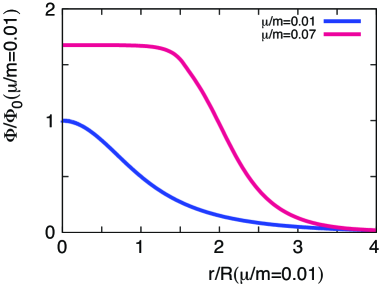
(a) Left Panel

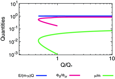
(b) Right Panel

Figure 1: Left Panel shows the profile of I/Q-ball for $\mu=0.01m$ and $\mu=0.07m$ for $\lambda=0.1,g=\lambda^{2}$ normalized by values at $\mu=0.01m$. Right Panel shows several dimensionless quantities of I/Q-ball for $\lambda=0.1,g=\lambda^{2}$ as a function of normalized charge $Q/Q_{\ast}$

Next, suppose that the real scalar field theory has the following potential:

$$V(\phi)=-\frac{1}{2}m^{2}(\phi_{0})\phi^{2}K\ln\left[\frac{\phi^{2}}{\phi_{0}^{2}}\right],$$ (3.10)

where $K$ comes from a one-loop correction which is assumed to be small and positive, $0<K\ll 1$, and $m^{2}(\phi_{0})$ is the mass defined at the scale $\phi_{0}$. Here and hereafter we write the mass term as $m^{2}=m^{2}(\phi_{0})$ unless otherwise stated. The corresponding complex scalar field theory with a conserved global U(1) symmetry has a following potential:

$$V_{\text{U(1)}}(|\Phi|)=-m^{2}|\Phi|^{2}K\ln\left[\frac{|\Phi|^{2}}{\Phi_{0}^{2}}\right];~{}~{}\Phi_{0}^{2}\equiv c\phi_{0}^{2},$$ (3.11)

with $c$ being a numerical constant given by $4/e$. Thus, Eq. (3.2) reads

$$\left[\frac{\partial^{2}}{\partial r^{2}}+\frac{2}{r}\frac{\partial}{\partial r}\right]\tilde{\Psi}=-\left(m^{2}-2\mu m\right)\tilde{\Psi}+m^{2}\tilde{\Psi}\left(1-K-K\ln\left[\frac{\tilde{\Psi}^{2}}{\Phi_{0}^{2}}\right]\right).$$ (3.12)

Since this potential satisfies the condition Eq. (3.4) as long as $K>0$, there is a non-trivial solution with boundary conditions Eq. (3.3). It is known that the solution can be well approximated by the Gaussian form in this case. Thus, the Q-ball solution has the following form

$$\Phi_{Q}(t,r)=e^{-i(m-\mu)t}\tilde{\Psi}_{G}(r);~{}~{}\tilde{\Psi}_{G}(r)=\Phi_{0}\exp\left[-\frac{r^{2}}{2R^{2}}\right],$$ (3.13)

where

$$mR=K^{-1/2};~{}~{}\mu=-Km,$$ (3.14)

which satisfy the non-relativistic condition: $1/R\ll m$ and $\mu\ll m$. Note that this relation is consistent with the rough estimation given in Eq. (3.5). One can see that if the amplitude is large enough, the Q-ball solution is energetically favored by considering the effective mass outside the Q-ball solution. Suppose that the typical energy scale outside the Q-ball solution is $\Lambda$, the effective mass outside $m(\Lambda)$ can be written as

$$m^{2}(\Lambda)\simeq m^{2}(\Phi_{0})\left(1+K\ln\left[\frac{\Phi_{0}^{2}}{\Lambda^{2}}\right]\right).$$ (3.15)

If the amplitude $\Phi_{0}$ is larger than $\Lambda$ so that $\ln(\Phi_{0}/\Lambda)>1$, the condition $m(\Phi_{0})-\mu<m(\Lambda)$ is satisfied and the Q-ball solution is energetically favored for a positive $K$. Contrary to the narrow regime in the polynomial potential, since the radius is given by $R\propto m(\Phi_{0})^{-1}$, the frequency of I/Q-ball, $\omega\sim m(\Phi_{0})$, decreases as the charge increases, $Q\propto m(\Phi_{0})\Phi_{0}^{2}R^{3}\propto(\Phi_{0}/m(\Phi_{0}))^{2}$. The I-ball solution reads

$$\phi_{I}(t,r)=\cos\left[\left(m-\mu\right)t\right]\tilde{\Phi}_{G}(r).$$ (3.16)

Note that if one defines the amplitude of I-ball solution as a square root of oscillation time average of $\phi_{I}^{2}$, the amplitude becomes

$$\sqrt{\overline{\phi_{I}^{2}}}=\frac{\Phi_{0}}{\sqrt{2}}\exp\left[-\frac{r^{2}}{2R^{2}}\right],$$ (3.17)

which is used in Ref. [31].

4 Stability of I-balls

Up to here, we have seen that the I-ball can be regarded as a non-topological soliton associated with the approximate U(1) conservation as long as the non-relativistic condition is maintained. However, after the formation of I-ball, if small fluctuations around the I-ball solution grow rapidly, such relativistic modes break the condition and hence the stability of I-ball is lost. Therefore, in this section, we discuss the robustness of the non-relativistic condition around the I-ball solution, which is verified if the effects from $V_{\rm B}(\Phi,\Phi^{\dagger})$ term are negligible.

Before going into details, it is instructive to recall the stability of Q-balls. Once one finds the bounce solution $\tilde{\Psi}_{B}$, its energy in the complex scalar field theory can be obtained from Eq. (2.13) as

$$E_{\text{Q-ball}}=\int 4\pi r^{2}dr\left[\left(m-\mu\right)^{2}\tilde{\Psi}_{B}^{2}+\left(\frac{\partial}{\partial r}\tilde{\Psi}_{B}\right)^{2}+V_{\text{U(1)}}(\tilde{\Psi}_{B})\right],$$ (4.1)

and its charge as

$$Q=2(m-\mu)\int 4\pi r^{2}dr\tilde{\Psi}_{B}^{2}.$$ (4.2)

The Q-ball solution is stable only if its energy is smaller than that of free particles:

$$E_{\text{Q-ball}}<mQ.$$ (4.3)

Intuitively, this condition indicates that the effective mass of the Q-ball solution is smaller than that of a free particle. The shallowness of the potential ensures this condition. For instance, in the case of the gravity mediation type potential, its energy and charge are given by

$$E_{\text{Q-ball}} =2\pi^{3/2}\left(1+\frac{5}{2}K\right)m^{2}(\phi_{0})\Phi_{0}^{2},$$ (4.4)

$$Q =2\pi^{3/2}\left(1+K\right)m(\phi_{0})\Phi_{0}^{2}R^{3}.$$ (4.5)

As explained in the previous section, as long as the typical scale of background plasma $\Lambda$ is much smaller than $\phi_{0}$, the condition (4.3) is satisfied

$$E_{\text{Q-ball}}\simeq m(\phi_{0})Q\left(1+\frac{3}{2}K\right)<m(\Lambda)Q,$$ (4.6)

because $m(\Lambda)<m(\phi_{0})$ for a positive $K$.

Then, let us discuss the stability of the corresponding I-ball. Once it is guaranteed that the non-relativistic condition holds, the I-ball solution can be obtained from that of the corresponding Q-ball and hence it becomes (quasi-)stable as long as Eq. (4.3) is met. To justify this statement, we have to verify that small fluctuations around the I-ball solution, $\delta\Phi$, does not grow violently due to the charge violating term $V_{\rm B}$, since otherwise such modes immediately break the non-relativistic condition. One can obtain the equation of motion for $\delta\Phi\equiv\Phi-\Phi_{Q}$ from Eq. (2.4) as

$$\left(\Box+m^{2}\right)\delta\Phi=-\left.\frac{\partial V^{\text{(int)}}}{\partial\Phi^{\dagger}}\right|_{\Phi=\Phi_{Q}+\delta\Phi}+\left.\frac{\partial V_{\rm U(1)}}{\partial\Phi^{\dagger}}\right|_{\Phi=\Phi_{Q}},$$ (4.7)

where we denote the full interaction except for the mass term as $V^{\text{(int)}}=V_{\rm U(1)}(|\Phi|)+V_{\rm B}(\Phi,\Phi^{\dagger})$.

To make our discussion concrete, let us for example see $\phi^{4}$ theory: $V^{\text{(int)}}=-(3\lambda/8)|\Phi|^{4}-(\lambda/16)(\Phi^{4}+{\Phi^{\dagger}}^{4})$. Then, the equation of motion for $\delta\Phi$ can be written as

$$\left(\Box+m^{2}\right)\delta\Phi=\frac{3\lambda}{2}|\Phi_{Q}|^{2}\delta\Phi+\frac{\lambda}{4}{\Phi^{\dagger}_{Q}}^{3}+\frac{3\lambda}{4}\left(\Phi_{Q}^{2}+{\Phi_{Q}^{\dagger}}^{2}\right)\delta\Phi^{\dagger}+O(\delta\Phi^{2}),$$ (4.8)

at the leading order in $\delta\Phi$. Note that $\delta\Phi=0$ does not satisfy the equation of motion because the rapidly oscillating $V_{B}$ term, $\lambda{\Phi_{Q}^{\dagger}}^{3}$, remains. Thus, we separate $\delta\Phi$ into $\delta\Phi_{\rm cmp}$ and $\delta\Phi_{\rm flc}$, and assume $\delta\Phi_{\rm cmp}$ compensates this term inside the I-ball. In the case of the $\phi^{4}$ potential, $\delta\Phi_{\rm cmp}$ can be estimated as a solution of the following equation

$$\left(\Box+m^{2}-\frac{3\lambda}{2}|\Phi_{Q}|^{2}\right)\delta\Phi_{\text{cmp}}\simeq\frac{\lambda}{4}{\Phi^{\dagger}_{Q}}^{3}.$$ (4.9)

$\delta\Phi_{\text{cmp}}$ simply oscillates with a frequency $3(m-\mu)$ inside the I-ball, and does not grow violently. A typical amplitude of the solution can be estimated as $|\delta\Phi_{\text{cmp}}|\sim(\lambda\Phi_{0}^{2}/m^{2})\Phi_{0}\ll\Phi_{0}$, which justifies the approximation we used, $|\Phi_{Q}|\gg|\delta\Phi|$. Note that in general $|\delta\Phi_{\rm cmp}|\sim|V^{\prime}_{\rm B}(\Phi_{Q},\Phi^{\dagger}_{Q})|/m^{2}\ll\Phi_{0}$ is ensured by the non-relativistic condition:

$$\left|V^{\prime}_{\rm B}(\Phi_{Q},\Phi^{\dagger}_{Q})\right|\sim\left|V^{\prime}_{\rm U(1)}(|\Phi_{Q}|)\right|\ll m^{2}|\Phi_{Q}|.$$ (4.10)

Hence, $\Phi_{\text{cmp}}$ does not threaten the non-relativistic condition. Here we omit effects from $\lambda(\Phi_{Q}^{2}+{\Phi_{Q}^{\dagger}}^{2})\delta\Phi_{\text{cmp}}^{\dagger}$ that may produce flux of relativistic particles from the I-ball. Its effects are discussed in the following as $\delta\Phi_{\text{flc}}$.

Then, let us focus on remaining modes defined as $\delta\Phi_{\text{flc}}$, which might break the non-relativistic condition. The equation of motion for $\delta\Phi_{\text{flc}}$ is given by

$$\left(\Box+m^{2}-\frac{3\lambda}{2}|\Phi_{Q}|^{2}\right)\delta\Phi_{\text{flc}}=\frac{3\lambda}{4}\left(\Phi_{Q}^{2}+{\Phi_{Q}^{\dagger}}^{2}\right)\delta\Phi_{\text{flc}}^{\dagger}.$$ (4.11)

Since the dispersion relation of $\delta\Phi_{\text{flc}}^{({\dagger})}$ oscillates with time due to the right hand side of Eq. (4.11), $\delta\Phi_{\text{flc}}^{({\dagger})}$ might grow exponentially due to the parametric resonance. Roughly speaking, this term may contain two classes of processes: number conserving processes ($2$ to $2$) as the first band and number violating processes ($n+m$ to $n$) as the higher band.

In the case of gravity mediation type potential, $V_{B}$ contains infinite series of terms as

$$V_{\rm B}=\frac{-m^{2}K}{6}\frac{\Phi^{4}+{\Phi^{\dagger}}^{4}}{|\Phi|^{2}}+\sum_{n\geq 3}c_{n}m^{2}K\frac{\Phi^{2n}+{\Phi^{\dagger}}^{2n}}{|\Phi|^{2n-2}},$$ (4.12)

with $c_{n}$ being a numerical constant (See Appendix. A). The interaction rate that comes from a higher power of $1/|\Phi|^{2}$ results in a higher power of $m/|\Phi_{Q}|$. Thus, if $m/|\Phi_{Q}|\ll 1$ holds, the expansion above is controlled. Here and hereafter, we assume $m/|\Phi_{Q}|\ll 1$ (in other words $\epsilon^{3}Q\gg 1$) in the case of gravity mediation type potential. The interaction terms for $\delta\Phi_{\rm flc}$ can be expressed as the following form

$$V\supset c\frac{Km^{2}}{|\Phi|^{2}}\frac{[\Phi_{Q}^{a}\text{ or }{{\Phi_{Q}^{\dagger}}^{a}}]}{|\Phi_{Q}|^{a}}\frac{(\delta\Phi_{\rm flc}\text{ or }\delta\Phi^{\dagger}_{\rm flc})^{b}}{|\Phi_{Q}|^{b-4}},$$ (4.13)

with non negative integer $a$, $b$ and numerical constant c. These interaction terms can cause both number conserving and number violating processes if they are energetically allowed.

The following of this section is devoted to show that, for sufficiently long time, effects of $\delta\Phi_{\rm flc}$ are negligible and the non-relativistic condition holds. We estimate the effects from $\delta\Phi_{\rm flc}$ focusing on particle production processes in two cases: the charge violating process of number conserving ($n$ to $n$) one and number changing ($n+m$ to $n$) one.

4.1 Number conserving processes

Let us consider charge violating but number conserving processes. In both polynomial potential and gravity mediation type potential, the U(1) violating term contains $V_{\text{B}}\supset(\Phi^{4}+{\Phi^{\dagger}}^{4})$, and hence charge violating but number conserving two to two processes $(++\rightarrow--)$ may happen.

The Q-ball solution with charge Q oscillates with a frequency $\omega(Q)\equiv m-\mu$. Thus, the produced particles in number conserving processes have energy $\omega(Q)$ per one particle. On the other hand, Q-ball solution with charge Q has energy $E_{\rm Q-ball}(Q)\simeq\omega(Q)Q$. Now, suppose that Q-ball solution loses its charge by $\triangle Q$ due to number conserving but charge violating processes. Then, the time-averaged total energy shifts to $\bar{E}^{\prime}$ that is roughly given by

$$\bar{E}^{\prime} \simeq\omega(Q-\triangle Q)\cdot[Q-\triangle Q]+\omega(Q)\triangle Q$$

$$\simeq\omega(Q)Q-\frac{\partial\omega(Q)}{\partial Q}Q\triangle Q$$

$$\geq\omega(Q)Q,$$ (4.14)

if the condition

$$\frac{\partial\omega(Q)}{\partial Q}<0,$$ (4.15)

is satisfied.

As explained before, in the case of gravity mediation potential, since the charge $Q$ is proportional to $Q\propto m(\Phi_{0})\Phi_{0}^{2}R^{3}\propto(\Phi_{0}/m(\Phi_{0}))^{2}$, the frequency of I/Q-ball $\omega\sim m(\Phi_{0})$ decreases as the charge increases. Therefore, the number conserving but charge violating processes are energetically unfavored.

On the other hand, in the case of polynomial potential, the frequency of I/Q-ball decrease as the charge increases in the flat-top regime similar to the case of gravity mediation potential but the opposite happens in the narrow regime (see Fig. 1(b)). Therefore, in the narrow regime, the charge violating but number conserving processes are energetically allowed. If such a process occurs effectively, the charge $Q$ drops down and the shape of the I-ball becomes sharper and sharper, which makes the non-relativistic condition worse and worse. Thus, in this regime, the collapse of I/Q-balls may be initiated by the charge violating but number conserving processes, and its time scale can be estimated as $\Gamma\sim\lambda\epsilon^{2}\omega$, which is much longer than the oscillation period as is consistent with [22, 36, 25].

4.2 Number changing processes

Now, we consider the number changing ($n+m$ to $n$) processes. First, let us consider the case of polynomial potential. Suppose a Q-ball solution with a size $R$, a wall width $L$, frequency $\omega$, and typical amplitude $\Phi_{0}$. Using relations Eq. (3.5), (4.2) and $\Phi_{0}^{2}\sim\lambda/g$ for flat-top regime, the followings hold

$$Q \sim\omega R^{3}\Phi_{0}^{2},$$ (4.16)

$$\epsilon \equiv 1/L\omega\sim\begin{cases}1/Rm~{}~{}\text{for narrow regime}\\ \lambda/\sqrt{g}~{}~{}\text{for flat-top regime}\end{cases},$$ (4.17)

$$\lambda\Phi_{0}^{2} \sim\epsilon^{2}m^{2}~{}~{}\text{for both regimes}.$$ (4.18)

Recall that the parameter $\epsilon\equiv 1/L\omega$ is small in general [See Eq. (3.6)]. In the case of polynomial potential, the dominant charge violating channel is a four to two process with $(++++\rightarrow+-)$ caused by quartic interaction term or sixtic one. For produced modes which have momenta compatible with $2\omega$, the size $R$ and the typical wall width $L$ are rather large. Thus, the number changing particle production processes which have typical length scales $\sim 1/\omega$ may not be sensitive to the spatial variations of the amplitude $\partial\ln\Phi/\partial r\sim 1/L\ll\omega$. Therefore, for simplicity, we approximate that the background condensation is spatially homogeneous in the following analysis. The four to two rate in the homogeneous background condensation can be calculated by, for example, using a method developed in [38]. We can estimate the decay rate of Q-ball charge as

$$\frac{dQ}{dt}\sim-\lambda\epsilon^{6}\omega Q,$$ (4.19)

for quartic interaction and

$$\frac{dQ}{dt}\sim-\lambda\epsilon^{6}\left(\frac{g}{\lambda^{2}}\right)^{2}\omega Q,$$ (4.20)

for sixtic interaction. Finally one can get typical decay rate by this process as

$$\Gamma_{I,4\rightarrow 2}\sim\begin{cases}\lambda\epsilon^{6}\omega~{}~{}~{}~{}\text{by quartic interaction}\\ \lambda\epsilon^{6}\left(\frac{g}{\lambda^{2}}\right)^{2}\omega\lesssim\lambda\epsilon^{2}\omega~{}~{}\text{by sixtic interaction}\end{cases},$$ (4.21)

which is suppressed by factors on $\lambda$ and $\epsilon$ compared to the frequency of I-ball. This result agrees with oscillon decay rate with a quartic or sixtic interaction estimated in [36]. One can say that smallness of the parameter $\epsilon\equiv 1/L\omega$, which is a consequence of the non-relativistic condition, ensures the approximate stability of I-ball.

Let us see the case of gravity mediation type potential. In this case, interaction terms have the form of (4.13). Using dimensional analysis we can estimate typical decay rate as

$$\Gamma_{\rm typ}\sim\frac{\epsilon^{1+4d}}{Q}(\epsilon^{3}Q)^{-e}\omega,$$ (4.22)

with non negative integer $d$ and $e$ depending on the interactions. The largest rate comes from the reaction $(++++\rightarrow++)$ with vertex $\sim Km^{2}\Phi^{6}/|\Phi|^{2}$ with $d=e=0$. With $\epsilon^{3}Q\gg 1$, the rate above is highly suppressed.

5 Discussion and Conclusions

In a non-relativistic configuration, a classical real scalar field theory can be embedded into a complex one with a conserved U(1) charge. From this fact, we have shown that an I-ball can be understood as a projection of a Q-ball, and that if the non-relativistic condition holds, the stability of I-ball is guaranteed by that of Q-ball. We have discussed the robustness of the non-relativistic condition and confirmed the long-lived nature of I-ball. Interestingly, we have seen that the main processes which determine a lifetime of the I/Q-ball may depend on the property of its frequency as a function of charge, $\omega(Q)$: number conserving processes are unfavored/favored for $\partial\omega/\partial Q\lessgtr 0$.

As one can guess, the separation of time scale plays a crucial role in the formation of I-ball. If one prepares inhomogeneous non-relativistic real scalar fields with a potential nearly but shallower than quadratic, they first fragment into I-balls if the non-relativistic condition is maintained for sufficiently long time. Then, they gradually reduce their number by producing relativistic particles, and the system finally relaxes into thermal equilibrium.

In more realistic situations, the background space-time expands, and a real scalar field may interact with light particles which participate in the background thermal plasma. On the one hand, since the momenta of scalar fields decrease due to the expansion of the Universe, the non-relativistic condition is expected to be satisfied easily. On the other hand, the interaction with the background plasma might make the scalar field energetic, and eventually the I-ball may evaporate [39]. It is also interesting to pursue, with what initial conditions and external force that deviates the system from thermal equilibrium (e.g., the cosmic expansion), the scalar field first fragments into the I-ball not into thermal equilibrium particles [40, 41, 32, 33]. We will return to these issues elsewhere.

Appendix A Embedding a real scalar field theory into complex one

We consider a real scalar $\phi$ field theory with the potential $V(2\phi^{2})$. The equation of motion is the following

$$\Box\phi+4V^{\prime}(2\phi^{2})\phi=0.$$ (A.1)

Now, we introduce a complex field $\Phi$ which satisfies $\Re(\Phi)=\phi$. The following holds

$$4V^{\prime}(2\phi^{2})\phi=2V^{\prime}\left(|\Phi|^{2}+\frac{\Phi^{2}+{\Phi^{\dagger}}^{2}}{2}\right)\cdot(\Phi+\Phi^{\dagger}).$$ (A.2)

By expanding the potential around $|\Phi|^{2}$, one can obtain the following form

$$4V^{\prime}(2\phi^{2})\phi =2V^{\prime}\left(|\Phi|^{2}+\frac{\Phi^{2}+{\Phi^{\dagger}}^{2}}{2}\right)(\Phi+\Phi^{\dagger})$$

$$=\sum_{n}k_{n}(|\Phi|^{2})\left(\frac{\Phi^{2}+{\Phi^{\dagger}}^{2}}{2}\right)^{n}(\Phi+\Phi^{\dagger})$$

$$=\sum_{n}g_{n}(|\Phi|^{2})\left[\Phi^{2n+1}+{\Phi^{\dagger}}^{2n+1}\right],$$ (A.3)

with some functions $k_{n}$ and $g_{n}$. Suppose $\Phi=re^{i\theta}$, we have

$$2rV^{\prime}\left(r^{2}(1+\cos 2\theta)\right)\cos\theta=\sum_{n}g_{n}(r^{2})\cos((2n+1)\theta)r^{2n+1}.$$ (A.4)

From this expression, we can calculate the function $g_{n}(x)$

$$g_{n}(r^{2})=\frac{2}{\pi}\int_{-\pi}^{\pi}\frac{V^{\prime}\left(r^{2}(1+\cos 2\theta)\right)\cdot\cos\theta\cdot\cos((2n+1)\theta)}{r^{2n}}d\theta.$$ (A.5)

On the other hand, the equation of motion can be rewritten as

$$\Re\left[\Box\Phi+\sum_{n}g_{n}(|\Phi|^{2})\left(\Phi^{2n+1}+{\Phi^{\dagger}}^{2n+1}\right)\right]+\Re\left[\sum_{n}f_{n}(|\Phi|^{2})\left(\Phi^{2n+1}-{\Phi^{\dagger}}^{2n+1}\right)\right]=0,$$ (A.6)

with arbitrary functions $f_{n}(x)$ because the last term vanishes. We can consider a complex scalar equation of motion

$$\Box\Phi+\sum_{n}\left[g_{n}(|\Phi|^{2})+f_{n}(|\Phi|^{2})\right]\Phi^{2n+1}+\sum_{n}\left[g_{n}(|\Phi|^{2})-f_{n}(|\Phi|^{2})\right]{\Phi^{\dagger}}^{2n+1}=0.$$ (A.7)

This equation of motion can be derived from the potential $G(\Phi,\Phi^{\dagger})$ which satisfies

$$G(\Phi,\Phi^{\dagger}) =\sum_{n}G_{n}(|\Phi|^{2})\left[\Phi^{2n}+{\Phi^{\dagger}}^{2n}\right],$$ (A.8)

$$g_{n}(x)+f_{n}(x) =G^{\prime}_{n}(x),$$ (A.9)

$$g_{n}(x)-f_{n}(x) =xG^{\prime}_{n+1}(x)+2(n+1)G_{n+1}(x),$$ (A.10)

$$G_{1}(x) =0.$$ (A.11)

With condition $G_{1}(x)=0$, we can compute $f_{n}$ and $G_{n}$. This is because $G_{n+1}$ can be determined by

$$2(n+1)G_{n+1}(x)+xG^{\prime}_{n+1}(x)=2g_{n}(x)-G^{\prime}_{n}(x).$$ (A.12)

Now, we have the charge conserving potential $V_{\rm U(1)}$ and violating term $V_{\rm B}$ as

$$V_{\rm U(1)}(|\Phi|^{2}) \equiv G_{0}(|\Phi|^{2}),$$ (A.13)

$$V_{\rm B}(\Phi,\Phi^{\dagger}) \equiv\sum_{n\geq 2}G_{n}(|\Phi|^{2})\left[\Phi^{2n}+{\Phi^{\dagger}}^{2n}\right].$$ (A.14)

For example, in the case of polynomial potential $V(x)=Ax^{m+1}/(m+1)$ with constant A, $G_{n}(x)$ can be obtained as

$$G_{n}(x)=2^{2-m}A\frac{1+(-1)^{n}}{2}\frac{{}_{2m+1}\mathrm{C}_{m-n+1}}{m+n+1}x^{m+1-n}\text{ for $n\leq m+1$ otherwise zero.}$$ (A.15)

References

- [1] A. H. Guth, Phys. Rev. D 23, 347-356 (1981); A. A. Starobinsky, Phys. Lett. B 91 (1980) 99; K. Sato, Mon. Not. Roy. Astron. Soc. 195, 467-479 (1981).
- [2] A. D. Linde, Phys. Lett. B 108 (1982) 389; A. Albrecht and P. J. Steinhardt, Phys. Rev. Lett. 48, 1220 (1982).
- [3] P. A. R. Ade et al. [Planck Collaboration], arXiv:1303.5076 [astro-ph.CO].
- [4] I. Affleck and M. Dine, Nucl. Phys. B 249, 361 (1985).
- [5] S. R. Coleman, Nucl. Phys. B 262, 263 (1985) [Erratum-ibid. B 269, 744 (1986)].
- [6] A. Kusenko and M. E. Shaposhnikov, Phys. Lett. B 418, 46 (1998) [hep-ph/9709492].
- [7] K. Enqvist and J. McDonald, Phys. Lett. B 425, 309 (1998) [hep-ph/9711514].
- [8] K. Enqvist and J. McDonald, Nucl. Phys. B 538, 321 (1999) [hep-ph/9803380].
- [9] S. Kasuya and M. Kawasaki, Phys. Rev. D 61, 041301 (2000) [hep-ph/9909509].
- [10] S. Kasuya and M. Kawasaki, Phys. Rev. D 62, 023512 (2000) [hep-ph/0002285].
- [11] S. Kasuya and M. Kawasaki, Phys. Rev. D 64, 123515 (2001) [hep-ph/0106119].
- [12] P. A. R. Ade et al. [BICEP2 Collaboration], arXiv:1403.3985 [astro-ph.CO].
- [13] I. L. Bogolyubsky and V. G. Makhankov, JETP Lett. 24, 12 (1976).
- [14] M. Gleiser, Phys. Rev. D 49, 2978 (1994) [hep-ph/9308279].
- [15] E. J. Copeland, M. Gleiser and H. -R. Muller, Phys. Rev. D 52, 1920 (1995) [hep-ph/9503217].
- [16] M. Gleiser and A. Sornborger, Phys. Rev. E 62, 1368 (2000) [patt-sol/9909002].
- [17] E. P. Honda and M. W. Choptuik, Phys. Rev. D 65, 084037 (2002) [hep-ph/0110065].
- [18] M. Gleiser, Phys. Lett. B 600, 126 (2004) [hep-th/0408221].
- [19] G. Fodor, P. Forgacs, P. Grandclement and I. Racz, Phys. Rev. D 74, 124003 (2006) [hep-th/0609023].
- [20] M. Hindmarsh and P. Salmi, Phys. Rev. D 74, 105005 (2006) [hep-th/0606016].
- [21] P. M. Saffin and A. Tranberg, JHEP 0701, 030 (2007) [hep-th/0610191].
- [22] G. Fodor, P. Forgacs, Z. Horvath and A. Lukacs, Phys. Rev. D 78, 025003 (2008) [arXiv:0802.3525 [hep-th]].
- [23] G. Fodor, P. Forgacs, Z. Horvath and M. Mezei, Phys. Rev. D 79, 065002 (2009) [arXiv:0812.1919 [hep-th]].
- [24] M. Gleiser and D. Sicilia, Phys. Rev. D 80, 125037 (2009) [arXiv:0910.5922 [hep-th]].
- [25] M. A. Amin and D. Shirokoff, Phys. Rev. D 81, 085045 (2010) [arXiv:1002.3380 [astro-ph.CO]].
- [26] M. A. Amin, R. Easther, H. Finkel, R. Flauger and M. P. Hertzberg, Phys. Rev. Lett. 108, 241302 (2012) [arXiv:1106.3335 [astro-ph.CO]].
- [27] P. Salmi and M. Hindmarsh, Phys. Rev. D 85, 085033 (2012) [arXiv:1201.1934 [hep-th]].
- [28] E. A. Andersen and A. Tranberg, JHEP 1212, 016 (2012) [arXiv:1210.2227 [hep-ph]].
- [29] M. Kawasaki and N. Takeda, arXiv:1310.4615 [astro-ph.CO].
- [30] P. M. Saffin, P. Tognarelli and A. Tranberg, arXiv:1401.6168 [hep-ph].
- [31] S. Kasuya, M. Kawasaki and F. Takahashi, Phys. Lett. B 559, 99 (2003) [hep-ph/0209358].
- [32] J. Berges and J. Jaeckel, arXiv:1402.4776 [hep-ph].
- [33] S. Davidson, arXiv:1405.1139 [hep-ph].
- [34] S. R. Coleman, V. Glaser and A. Martin, Commun. Math. Phys. 58, 211 (1978).
- [35] K. Enqvist and M. Laine, JCAP 0308, 003 (2003) [cond-mat/0304355].
- [36] M. P. Hertzberg, Phys. Rev. D 82, 045022 (2010) [arXiv:1003.3459 [hep-th]].
- [37] M. Kawasaki and M. Yamada, arXiv:1311.0985 [hep-ph].
- [38] S. Matsumoto and T. Moroi, Phys. Rev. D 77, 045014 (2008) [arXiv:0709.4338 [hep-ph]].
- [39] K. Mukaida and K. Nakayama, JCAP 1301, 017 (2013) [arXiv:1208.3399 [hep-ph]].
- [40] J. Berges and D. Sexty, Phys. Rev. Lett. 108, 161601 (2012) [arXiv:1201.0687 [hep-ph]].
- [41] B. Nowak, S. Erne, M. Karl, J. Schole, D. Sexty and T. Gasenzer, arXiv:1302.1448 [cond-mat.quant-gas].