A monolithic multi-time-step computational
framework for first-order transient systems
with disparate scales
   
An e-print of the paper is available on arXiv: http://arxiv.org/abs/1405.3230.

Authored by

S. Karimi

Graduate Student, University of Houston.

K. B. Nakshatrala

Department of Civil & Environmental Engineering
University of Houston, Houston, Texas 77204–4003.
phone: +1-713-743-4418, e-mail: knakshatrala@uh.edu
website: http://www.cive.uh.edu/faculty/nakshatrala

Abstract.

Developing robust simulation tools for problems involving multiple mathematical scales has been a subject of great interest in computational mathematics and engineering. A desirable feature to have in a numerical formulation for multiscale transient problems is to be able to employ different time-steps (multi-time-step coupling), and different time integrators and different numerical formulations (mixed methods) in different regions of the computational domain. To this end, we present two new monolithic multi-time-step mixed coupling methods for first-order transient systems. We shall employ unsteady advection-diffusion-reaction equation with linear decay as the model problem, which offers several unique challenges in terms of non-self-adjoint spatial operator and rich features in the solutions. We shall employ the dual Schur domain decomposition technique to split the computational domain into an arbitrary number of subdomains. It will be shown that the governing equations of the decomposed problem, after spatial discretization, will be differential/algebraic equations. This is a crucial observation to obtain stable numerical results. Two different methods of enforcing compatibility along the subdomain interface will be used in the time discrete setting. A systematic theoretical analysis (which includes numerical stability, influence of perturbations, bounds on drift along the subdomain interface) will be performed. The first coupling method ensures that there is no drift along the subdomain interface, but does not facilitate explicit/implicit coupling. The second coupling method allows explicit/implicit coupling with controlled (but non-zero) drift in the solution along the subdomain interface. Several canonical problems will be solved to numerically verify the theoretical predictions, and to illustrate the overall performance of the proposed coupling methods. Finally, we shall illustrate the robustness of the proposed coupling methods using a multi-time-step transient simulation of a fast bimolecular advective-diffusive-reactive system.

1. INTRODUCTION AND MOTIVATION

Advection-diffusion-reaction equations can exhibit several mathematical (i.e., temporal and spatial) scales depending on the relative strengths of advection, diffusion and reaction processes, and on the strength of the volumetric source/sink. The presence of these mathematical scales is evident from the qualitative richness that the solutions of advection-diffusion-reaction equations exhibit. For example, it is well-known that solutions to advection-dominated problems typically exhibit steep gradients near the boundaries [Gresho and Sani, 2000]. Solutions to diffusion-dominated problems tend to be diffusive and smooth [McOwen, 1996], whereas reaction-dominated solutions typically exhibit sharp fronts and complex spatial patterns [Walgraef, 1997]. These scales can be systematically characterized using the well-known non-dimensional numbers – the Péclet number and the Damköhler numbers [Bird et al., 2006]. It needs to be emphasized that these equations, in general, are not amenable to analytical solutions. Therefore, one has to rely on predictive numerical simulations for solving problems of any practical relevance. Due to the presence of disparate mathematical scales in these systems, it is highly desirable to have a stable computational framework that facilitates tailored numerical formulations in different regions of the computational domain.

Several advances have been made in developing numerical formulations for advection-diffusion-reaction equations, especially in the area of stabilized formulations [Codina, 2000; Augustin et al., 2011], and in the area of discrete maximum principles [Burman and Ern, 2002]. However, the main research challenge that still remains is to develop numerical methodologies for these type of problems to adequately resolve different mathematical scales in time and in space. This paper precisely aims at addressing this issue by developing a stable multi-time-step coupling framework for first-order transient systems that allows different time-steps, different time integrators and different numerical formulations in different regions of a computational domain.

Most of the prior works on multi-time-step coupling methods have focused on the second-order transient systems arising in the area of structural dynamics (e.g., see the discussion in [Karimi and Nakshatrala, 2014], and references therein). Some attempts regarding time integration of partitioned first-order systems can be found in [Nakshatrala et al., 2008, 2009]. In [Nakshatrala et al., 2008], a staggered multi-time-step coupling method is proposed. This method is considered as a staggered scheme as the Lagrange multipliers are calculated in an explicit fashion (i.e., based on the quantities known at prior time-levels). The stability and accuracy (especially, the control of drift along the subdomain interface) have been improved through the use of projection methods at appropriate time-levels. Since the method is a staggered scheme the obvious drawback is that the overall accuracy is first-order. However, it needs to be emphasized that the method proposed in [Nakshatrala et al., 2008] has better accuracy and stability properties than the previously proposed staggered schemes (e.g., [Piperno et al., 1995; Piperno, 1997]). In [Nakshatrala et al., 2009], several monolithic schemes are discussed for first-order transient systems but the treatment is restricted to transient diffusion equations (i.e., self-adjoint spatial operators) and multi-time-stepping was not addressed. Motivated by the work of Akkasale [Akkasale, 2011]; in which it has been systematically shown that many popular staggered schemes (e.g., [Piperno et al., 1995; Piperno, 1997]) suffer from numerical instabilities for both first- and second-order transient systems; we herein choose a monolithic approach to develop coupling methods that allow multi-time-steps.

Recently, a multi-time-step monolithic coupling method for linear elastodynamics, which is a second-order transient system, has been proposed in [Karimi and Nakshatrala, 2014]. However, developing a multi-time-step coupling method for first-order transient systems (e.g., unsteady advection-diffusion and advection-diffusion-reaction equations) will bring unique challenges. To name a few:

1. As shown in [Karimi and Nakshatrala, 2014], coupling explicit and implicit time-stepping schemes is always possible in the case of second-order transient systems. We will show later in this paper that such coupling is not always possible for first-order transient systems, and can be achieved only if an appropriate stabilized form of the interface continuity constraint is employed. We will also show that this explicit/implicit coupling for first-order transient systems will come at an expense of controlled drift.

2. Spatial operators in advection-diffusion-reaction equations are not self-adjoint. Symmetry and positive definiteness of the discretized operators should be carefully examined to ensure the stability of multi-time-step coupling methods. For second-order transient systems, the overall stability of the coupling method can be achieved provided the stability criterion in each subdomain is satisfied (which depends on the choice of the time-stepping scheme in the subdomain and the choice of the subdomain time-step) [Karimi and Nakshatrala, 2014]. We will show in a subsequent section that ensuring the stability of the time-stepping schemes in subdomains alone will not guarantee the overall stability of the coupling method. There is a need to place additional restrictions on the continuity constraints along the subdomain interface.

3. The governing equations of decomposed first-order transient systems form a system of differential/algebraic equations (DAEs) in Hessenberg form with a differential index 2. On the other hand, the governing equations for second-order transient systems form a system of DAEs with differential index 3. For more details on DAEs and associated terminology, see the brief discussion provided in subsection 3.1.1 or consult [Hairer and Wanner, 1996].

The current paper builds upon the ideas presented in [Nakshatrala et al., 2009; Karimi and Nakshatrala, 2014]. The central hypothesis on which the proposed multi-time-step coupling framework has been developed is two-fold: (i) The governing equations before the domain decomposition form a system of ordinary differential equations (ODEs). On the other hand, the governing equations resulting from the decomposition of the domain form a system of differential/algebraic equations. It needs to be emphasized that many of the popular time-stepping schemes (which are developed for solving ODEs) are not appropriate for solving DAEs [Gear and Petzold, 1984; Petzold, 1992]. At least, the accuracy and the stability properties will be altered considerably. The title of an influential paper in the area of numerical solutions of DAEs by Petzold [Petzold, 1982] clearly conveys the aforementioned sentiment: “Differential/algebraic equations are not ODEs.” Therefore, we shall take a differential/algebraic equations perspective in posing the governing equations of the decomposed problems, and apply time-stepping strategies that are appropriate to solve DAEs. (ii) Development and performance of multi-time-step coupling methods for first-order transient systems is different from that of second-order transient systems.

The proposed monolithic multi-time-step coupling framework for first-order transient systems enjoys several attractive features, which will be illustrated in the subsequent sections by both theoretical analysis and numerical results. In the remainder of this paper, we shall closely follow the notation introduced for multi-time-step coupling in [Karimi and Nakshatrala, 2014].

2. CONTINUOUS MODEL PROBLEM: TRANSIENT ADVECTION-DIFFUSION-REACTION EQUATION

We shall consider transient advection-diffusion-reaction equation as the continuous model problem. Our choice provides an ideal setting for developing multi-time-step coupling methods for first-order transient systems, as the governing equations pose several unique challenges. First, the relative strengths of advection, diffusion, reaction, and volumetric source introduce multiple temporal scales, which compel a need for a multi-time-step computational framework. Second, the spatial operator is not self-adjoint, which adds to the complexity of obtaining stability proofs. It needs to be emphasized that the current efforts on multi-time-step coupling have focused on second-order transient systems, and the stability analyses have been restricted to the cases in which the coefficient (i.e., “stiffness”) matrix is symmetric and positive definite [Karimi and Nakshatrala, 2014]. This will not be the case with respect to the advective-diffusive and advective-diffusive-reactive systems. Third, a numerical method to the chosen model problem can serve as a template for developing multi-time-step coupling methods for more complicated and important problems like transport-controlled bimolecular reactions, which exhibit complex spatial and temporal patterns. None of the prior works on multi-time-step coupling methods have undertaken such a comprehensive study, which this paper strives to achieve.

Consider a chemical species that is transported by both advection and diffusion processes, and simultaneously undergoes a chemical reaction. Let $\Omega\subset\mathbb{R}^{nd}$ denote the spatial domain, where “$nd$” denotes the number of spatial dimensions. The boundary is denoted by $\partial\Omega$, which is assumed to be piece-wise smooth. The gradient and divergence operators with respect to $\mathbf{x}\in\Omega$ are, respectively, denoted by $\mathrm{grad}[\cdot]$ and $\mathrm{div}[\cdot]$. The time is denoted by $t\in\mathcal{I}:=(0,T]$, where $\mathcal{I}$ is the time interval of interest. Let $c(\mathbf{x},t)$ denote the concentration of the chemical species. As usual, the boundary is divided into two parts: $\Gamma^{\mathrm{D}}$ and $\Gamma^{\mathrm{N}}$ such that $\Gamma^{\mathrm{D}}\cup\Gamma^{\mathrm{N}}=\partial\Omega$ and $\Gamma^{\mathrm{D}}\cap\Gamma^{\mathrm{N}}=\emptyset$. $\Gamma^{\mathrm{D}}$ is the part of the boundary on which concentration is prescribed (i.e., Dirichlet boundary condition), and $\Gamma^{\mathrm{N}}$ is that part of the boundary on which flux is prescribed (i.e., Neumann boundary condition). We shall denote the advection velocity vector field by $\mathbf{v}(\mathbf{x},t)$. The diffusivity tensor, which is a second-order tensor, is denoted by $\mathbf{D}(\mathbf{x})$, and is assumed to be symmetric and uniformly elliptic [Evans, 1998]. The initial boundary value problem for a transient advective-diffusive-reactive system can be written as follows:

$$\frac{\partial\mathrm{c}}{\partial t}+\mathrm{div}\left[\mathbf{v}\mathrm{c}-\mathbf{D}\left(\mathbf{x}\right)\mathrm{grad}[\mathrm{c}]\right]+\beta\mathrm{c}=f(\mathbf{x},t)\quad \mathrm{in}\;\Omega\times\mathcal{I}$$ (2.1a)

$$\mathrm{c}(\mathbf{x},t)=\mathrm{c}^{\mathrm{p}}(\mathbf{x},t)\quad \mathrm{on}\;\Gamma^{\mathrm{D}}\times\mathcal{I}$$ (2.1b)

$$- \widehat{\mathbf{n}}(\mathbf{x})\cdot\mathbf{D}(\mathbf{x})\mathrm{grad}[\mathrm{c}]=q^{\mathrm{p}}(\mathbf{x},t)\quad \mathrm{on}\;\Gamma^{\mathrm{N}}\times\mathcal{I}$$ (2.1c)

$$\mathrm{c}(\mathbf{x},t=0)=\mathrm{c}_{0}(\mathbf{x})\quad \mathrm{in}\;\Omega$$ (2.1d)

where $\widehat{\mathbf{n}}(\mathbf{x})$ denotes the unit outward normal to the boundary, $\mathrm{c}_{0}(\mathbf{x})$ is the prescribed initial concentration, $\mathrm{c}^{\mathrm{p}}(\mathbf{x},t)$ is the prescribed concentration on the boundary, $q^{\mathrm{p}}(\mathbf{x},t)$ is the prescribed diffusive flux on the boundary, $f(\mathbf{x},t)$ is the prescribed volumetric source/sink, and $\beta\geq 0$ is the coefficient of decay due to a chemical reaction.

As mentioned earlier, the mathematical scales in advective-diffusive-reactive systems can be characterized using popular non-dimensional numbers. A non-dimensional measure to identify the relative dominance of advection is the Péclet number, which can be defined as follows:

$$P_{e}(\mathbf{x},t):=\frac{L\|\mathbf{v}(\mathbf{x},t)\|}{D(\mathbf{x})}$$ (2.2)

where $L$ is the characteristic length, $D$ is the characteristic diffusivity, and $\|\cdot\|$ denotes the standard 2-norm. In the case of anisotropic diffusion tensor, $D(\mathbf{x})$ can be taken as the minimum eigenvalue of the diffusivity tensor at $\mathbf{x}$ (i.e., $D(\mathbf{x})=\mathrm{min}\left\{\kappa\;|\;\mathrm{det}\left(\mathbf{D}(\mathbf{x})-\kappa\mathbf{I}\right)=0\right\}$). Clearly, the higher the Péclet number the greater will be the relative dominance of advection. A non-dimensional quantity to measure the relative dominance of the chemical reaction is the Damköhler number, which takes the following form:

$$D_{a}:=\frac{\beta L^{2}}{D(\mathbf{x})}$$ (2.3)

In the context of numerical solutions, the characteristic length is typically associated with an appropriate measure of the mesh size. A popular choice under the finite element method is $L=h_{e}/2$, where $h_{e}$ is the diameter of the circumscribed circle of the element and the factor $1/2$ is for convenience. This choice gives rise to what is commonly referred to as the element Péclet number (e.g., see [Donea and Huerta, 2003]):

$$P_{e}^{h}=\frac{h_{e}\|\mathbf{v}(\mathbf{x},t)\|}{2D}$$ (2.4)

which will be used in subsequent sections, especially, in defining stabilized weak formulations. We shall employ the semi-discrete methodology [Zienkiewicz and Taylor, 1989] based on the finite element method for spatial discretization and the trapezoidal family of time-stepping schemes for the temporal discretization.

2.1. Trapezoidal family of time-stepping schemes

The time interval of interest is divided into $\mathcal{N}$ sub-intervals such that

$$\mathcal{I}=\left(0,T\right]=\bigcup_{n=1}^{\mathcal{N}}\left(t^{(n-1)},t^{(n)}\right]$$ (2.5)

where $t^{(0)}=0$ and $t^{(\mathcal{N})}=T$. To make the presentation simple, we shall assume that the sub-intervals are uniform. That is,

$$t^{(n)}-t^{(n-1)}=\Delta t\quad\forall n=1,\cdots,\mathcal{N}$$ (2.6)

where $\Delta t$ will be referred to as the time-step. However, it should be noted that the methods presented in this paper can be easily extended to variable time-steps. The primary variable (which, in our case, will be the concentration) and the corresponding time derivative at discrete time levels are denoted as follows:

$$d^{(n)}\approx\mathrm{c}(t=t^{(n)}),\quad v^{(n)}\approx\left.\frac{\partial\mathrm{c}}{\partial t}\right|_{t=t^{(n)}}$$ (2.7)

The trapezoidal family of time-stepping schemes can be compactly written as follows:

$$d^{(n+1)}=d^{(n)}+\Delta t\left((1-\vartheta)v^{(n)}+\vartheta v^{(n+1)}\right)$$ (2.8)

where $\vartheta\in[0,1]$ is a user-specified parameter. Some popular time-stepping schemes under the trapezoidal family include the explicit Euler ($\vartheta=0$, which is also known as the forward Euler), the midpoint rule $(\vartheta=1/2)$, and the implicit Euler ($\vartheta=1$, which is also known as the backward Euler). The forward Euler method is an explicit scheme, and the midpoint and the backward Euler schemes are implicit. The stability and accuracy properties of these time-stepping schemes in the context of ordinary differential equations are well-known (e.g., see [Hairer and Wanner, 2009]).

2.2. Weak formulations

We will now present several weak formulations for the initial boundary value problem given by equations (2.1a)–(2.1d), which will be used in the remainder of the paper. Since we address advection-dominated and reaction-dominated problems, we will present two popular stabilized weak formulations in addition to the Galerkin weak formulation. Let us introduce the following function spaces:

$$\mathsf{C}_{t} :=\left\{\mathrm{c}(\mathbf{x},\cdot)\in H^{1}(\Omega)\;|\;\mathrm{c}(\mathbf{x},t)=\mathrm{c}^{\mathrm{p}}(\mathbf{x},t)\;\mathrm{on}\;\Gamma^{\mathrm{D}}\right\}$$ (2.9a)

$$\mathsf{W} :=\left\{\mathrm{w}(\mathbf{x})\in H^{1}(\Omega)\;|\;\mathrm{w}(\mathbf{x})=0\;\mathrm{on}\;\Gamma^{\mathrm{D}}\right\}$$ (2.9b)

where $H^{1}(\Omega)$ is a standard Sobolev space [Brezzi and Fortin, 1991]. For convenience, we shall denote the standard $L_{2}$ inner-product over a set $K$ as follows:

$$\left(a;b\right)_{K}\equiv\int_{K}a\cdot b\;\mathrm{d}K$$ (2.10)

The subscript $K$ will be dropped if the set is the entire spatial domain (i.e., $K=\Omega$).

2.2.1. Galerkin weak formulation

The Galerkin formulation for the initial boundary value problem (2.1a)–(2.1d) can be written as follows: Find $\mathrm{c}(\mathbf{x},t)\in\mathsf{C}_{t}$ such that we have

$$\left(\mathrm{w};\partial\mathrm{c}/\partial t\right)+\left(\mathrm{w};\mathrm{div}[\mathbf{v}\mathrm{c}]\right)+\left(\mathrm{grad}[\mathrm{w}];\mathbf{D}(\mathbf{x})\mathrm{grad}[\mathrm{c}]\right)+(\mathrm{w};\beta\mathrm{c}-f)=\left(\mathrm{w};q^{\mathrm{p}}\right)_{\mathrm{\Gamma}^{\mathrm{N}}}\;\forall\mathrm{w}(\mathbf{x})\in\mathsf{W}$$ (2.11)

It is well-known that the Galerkin formulation may exhibit numerical instabilities (e.g., spurious node-to-node oscillations) for non-self-adjoint spatial operators like the advective-diffusive and advective-diffusive-reactive systems. The reason can be attributed to the presence of boundary layers and interior layers in the solutions of these systems when advection is more dominant than the diffusion and reaction processes. Designing stable numerical formulations for advection-diffusion and advection-diffusion-reaction problems is still an active area of research (e.g., see [Turner et al., 2011; Franca et al., 2006; Gresho and Sani, 2000]). This paper is not concerned with developing new stabilized formulations.

In order to avoid spurious oscillations and obtain accurate numerical solutions, it is sufficient to have the element Péclet number to be smaller than unity. To put it differently, if the element Péclet number is greater than unity, the computational mesh may not be adequate to resolve the steep gradients due to boundary layers and internal layers, which are typical in the solutions of advection dominated problems. One can always achieve smaller values for the element Péclet number by refining the computational mesh adequately. However, in some cases, the mesh has to be so fine that it may be computationally prohibitive to employ such a mesh. In order to alleviate the deficiencies of the Galerkin formulation for advection-dominated problems, many alternative methods have been proposed in the literature. For example, see [Augustin et al., 2011] for a short description and comparison of these methods. In this paper, we shall employ the SUPG formulation [Brooks and Hughes, 1982] and the GLS formulation [Hughes et al., 1989], which are two popular approaches employed to enhance the stability of the Galerkin formulation. For completeness and future reference, we now briefly outline these two stabilized formulations.

2.2.2. Streamline Upwind/Petrov-Galerkin (SUPG) weak formulation

The SUPG formulation reads as follows: Find $c(\mathbf{x},t)\in\mathsf{C}_{t}$ such that we have

$$(\mathrm{w};\partial\mathrm{c}/\partial t) +(\mathrm{w};\mathrm{div}[\mathbf{v}\mathrm{c}])+(\mathrm{grad}[\mathrm{w}];\mathbf{D}(\mathbf{x})\mathrm{grad}[\mathrm{c}])+(\mathrm{w};\beta\mathrm{c})$$

$$+\sum_{e=1}^{Nele}\left(\tau_{\mathrm{SUPG}}\mathbf{v}\cdot\mathrm{grad}[\mathrm{w}];\partial\mathrm{c}/\partial t+\mathrm{div}\left[\mathbf{v}\mathrm{c}-\mathbf{D}(\mathbf{x})\mathrm{grad}[\mathrm{c}]\right]+\beta\mathrm{c}-f\right)_{\Omega_{e}}$$

$$=(\mathrm{w};f)+\left(\mathrm{w};q^{\mathrm{p}}\right)_{\mathrm{\Gamma}^{\mathrm{N}}}\quad\forall\mathrm{w}(\mathbf{x})\in\mathsf{W}$$ (2.12)

where $Nele$ is the number of elements, and $\tau_{\mathrm{SUPG}}$ is the stabilization parameter under the SUPG formulation. We shall use the stabilization parameter proposed in [John and Knobloch, 2007]:

$$\tau_{\mathrm{SUPG}}=\frac{h_{e}}{2\|\mathbf{v}\|}\xi_{0}\left(P_{e}^{h}\right),\quad\xi_{0}\left(\chi\right)=\coth\left(\chi\right)-\frac{1}{\chi}$$ (2.13)

where $h_{e}$ is the element length, and $\xi_{0}$ is known as the upwind function. Recall that $P_{e}^{h}$ is the local (element) Péclet number.

2.2.3. Galerkin/least-squares (GLS) weak formulation

The GLS formulation reads as follows: Find $c(\mathbf{x},t)\in\mathsf{C}_{t}$ such that we have

$$(\mathrm{w};\partial\mathrm{c}/\partial t) +(\mathrm{w};\mathrm{div}[\mathbf{v}\mathrm{c}])+(\mathrm{grad}[\mathrm{w}];\mathbf{D}(\mathbf{x})\mathrm{grad}[\mathrm{c}])+(\mathrm{w};\beta\mathrm{c})$$

$$+\sum_{e=1}^{Nele}\left(\mathrm{w}/\Delta t+\mathrm{div}[\mathbf{v}\mathrm{w}-\mathbf{D}(\mathbf{x})\mathrm{grad}[\mathrm{w}]]+\beta\mathrm{w};\tau_{\mathrm{GLS}}\left(\partial\mathrm{c}/\partial t+\mathrm{div}\left[\mathbf{v}\mathrm{c}-\mathbf{D}(\mathbf{x})\mathrm{grad}[\mathrm{c}]\right]+\beta\mathrm{c}-f\right)\right)_{\Omega_{e}}$$

$$=(\mathrm{w};f)+\left(\mathrm{w};q^{\mathrm{p}}\right)_{\mathrm{\Gamma}^{\mathrm{N}}}\quad\forall\mathrm{w}(\mathbf{x})\in\mathsf{W}$$ (2.14)

where $\tau_{\mathrm{GLS}}$ is the stabilization parameter under the GLS formulation, and $\Delta t$ is the time-step. In this paper, we shall take $\tau_{\mathrm{GLS}}=\tau_{\mathrm{SUPG}}$, which is a common practice. It should be emphasized that an optimal choice of stabilization parameter for stabilized formulations in two- and three-dimensions is still an active area of research (e.g., see [Augustin et al., 2011]).

3. PROPOSED MULTI-TIME-STEP COMPUTATIONAL FRAMEWORK

The proposed multi-time-step computational framework is built upon the semi-discrete methodology [Zienkiewicz and Taylor, 1989] and the dual Schur domain decomposition method [Toselli and Widlund, 2004]. The semi-discrete methodology converts the partial differential equations into a system of ordinary differential equations. For spatial discretization of the problem at hand, one can use either the Galerkin formulation or a stabilized formulation, which could depend on the relative strengths of transport processes and the decay coefficient due to chemical reactions. The dual Schur domain decomposition is an elegant way to handle decomposition of the computational domain into subdomains through Lagrange multipliers.

3.1. Domain decomposition and the resulting equations

In order to facilitate multi-time-step coupling, we decompose the computational domain into $\mathcal{S}$ non-overlapping subdomains such that

$$\overline{\Omega}=\bigcup_{i=1}^{\mathcal{S}}\overline{\Omega}_{i}\quad\mathrm{and}\quad\Omega_{i}\cap\Omega_{j}=\emptyset\;\mathrm{for}\;i\neq j$$ (3.1)

where a superposed bar denotes the set closure. The meshes in all subdomains are assumed to be conforming along the subdomain interface, see Figure 1. We shall use signed Boolean matrices to write the compatibility constraints along the subdomain interface, as they provide a systematic way to write the interface constraints as a system of linearly independent equations. Moreover, the mathematical structure of the resulting equations is suitable for a mathematical analysis. The entries of a signed Boolean matrix are either -1, 0, or 1, and each row has at most one non-zero entry. However, it needs to be emphasized that a signed Boolean matrix is never constructed explicitly in a computer implementation, as it is computationally not efficient to store such a matrix. It should also be noted that signed Boolean matrices can handle constraints arising from cross-points, which are the points on the subdomain interface that are connected to more than two subdomains. For more details on signed Boolean matrices see [Nakshatrala et al., 2008].

In a time-continuous setting, the governing equations after spatial discretization can be written as follows:

$$\boldsymbol{M}_{i}\dot{\boldsymbol{c}}_{i}(t)+\boldsymbol{K}_{i}\boldsymbol{c}_{i}(t)=\boldsymbol{f}_{i}(t)+\boldsymbol{C}_{i}^{\mathrm{T}}\boldsymbol{\lambda}\left(t\right)\quad i=1,\cdots,\mathcal{S}$$ (3.2a)

$$\sum_{i=1}^{\mathcal{S}}\boldsymbol{C}_{i}\boldsymbol{c}_{i}\left(t\right)=\boldsymbol{0}$$ (3.2b)

where a superposed dot denotes a derivative with respect to time, the subscript $i$ denotes the subdomain number, the nodal concentration vector of the $i$-th subdomain is denoted by $\boldsymbol{c}_{i}$, the capacity matrix of the $i$-th subdomain is denoted by $\boldsymbol{M}_{i}$, the transport matrix of the $i$-th subdomain is denoted by $\boldsymbol{K}_{i}$, $\boldsymbol{f}_{i}(t)$ is the forcing vector of the $i$-th subdomain, $\boldsymbol{\lambda}$ denotes the vector of Lagrange multipliers, and $\boldsymbol{C}_{i}$ denotes the signed Boolean matrix for the $i$-th subdomain. Let the number of degrees-of-freedom in the $i$-th subdomain be denoted by $N_{i}$, and the number of degrees-of-freedom on the subdomain interface be denoted by $N_{\lambda}$. The size of $\boldsymbol{c}_{i}$ is $N_{i}\times 1$, and both the capacity and transport matrices of the $i$-th subdomain will be of the size $N_{i}\times N_{i}$. The size of $\boldsymbol{\lambda}$ will be $N_{\lambda}\times 1$, and the size of the signed Boolean matrix $\boldsymbol{C}_{i}$ will be $N_{\lambda}\times N_{i}$.

It is imperative to note that the governing equations (3.2a)–(3.2b), which arise from domain decomposition, form a system of differential/algebraic equations (DAEs). For completeness and future reference we now present the necessary details about differential/algebraic equations.

3.1.1. Differential/algebraic equations

A differential/algebraic equation is an equation involving a set of independent variables, an unknown function of the independent variables, and derivatives of the functions with respect to the independent variables. Clearly, ordinary differential equations, and algebraic equations form subclasses of differential/algebraic equations. In this paper, we are concerned with first-order differential/algebraic equations. Mathematically, a DAE in first-order form takes the following general form:

$$\boldsymbol{w}\left(\dot{\boldsymbol{x}}(t),\boldsymbol{x}\left(t\right),t\right)=\boldsymbol{0}\quad t\in\mathcal{I}$$ (3.3)

where $t$ is the independent variable, and $\boldsymbol{x}(t)$ is the unknown function. It is well-known that solving a system of differential/algebraic equations numerically can be more difficult than solving a system of ordinary differential equations [Hairer and Wanner, 1996; Petzold, 1982]. A notion which is popularly employed to measure the difficulty of obtaining numerical solutions to a particular DAE is the differential index. The differential index of a DAE is the number of times one has to take derivatives of equation (3.3) in order to be able to derive an ODE by mere algebraic manipulations. It is obvious that a system of ODEs will have differential index of zero. A special form of DAEs which is of interest to us in this paper is the Hessenberg index-2 DAE. It has the following mathematical form:

$$\dot{\boldsymbol{x}}=\boldsymbol{p}(\boldsymbol{x},\boldsymbol{y},t)$$ (3.4a)

$$\boldsymbol{0}=\boldsymbol{q}(\boldsymbol{x})$$ (3.4b)

which consists of a system of ordinary differential equations along with a set of algebraic equations (i.e., constraints). This paper concerns with differential/algebraic equations of differential index two or lower. Many of the constrained mechanical systems can be modeled using DAEs (e.g., see [Geradin and Cardona, 2001]). In the case of coupling algorithms, the compatibility of subdomains along the interfaces will appear as an algebraic constraint to the ODEs obtained from a finite element discretization. It is not possible to solve differential/algebraic equations analytically unless in some very special cases. Hence, one has to resort to numerical solutions. In this paper, we shall restrict to time-stepping schemes from the trapezoidal family. However, the corresponding properties when applied to differential/algebraic equations can be different. For a detailed discussion on this topic see [Hairer and Wanner, 1996].

3.2. Time discretization

We now construct two multi-time-step coupling methods that can handle multiple subdomains, and can allow the use of different time-steps, different time-integrators and/or different numerical formulation in different subdomains. To this end, the time interval of interest is divided into non-overlapping intervals whose end points will be referred to as system time-levels. The algebraic compatibility constraints will be enforced at the system time-levels. For convenience, we shall assume that the system time-levels are uniform. The $n$-th system time-level will be denoted by $t^{(n)}$ and can be written as follows:

$$t^{(n)}=n\Delta t\quad n=0,1,\cdots,\mathcal{N}$$ (3.5)

where $\Delta t$ is called the system time-step. The numerical time-integration of each subdomain will advance by the subdomain time-step. The subdomain time-step of the $i$-th subdomain will be denoted by $\Delta t_{i}$. Note that $\Delta t\geq\Delta t_{i}\;\forall i$. Furthermore, we shall assume that the ratio between the system and subdomain time-step is a natural number, and is denoted by $\eta_{i}$. That is,

$$\eta_{i}=\frac{\Delta t}{\Delta t_{i}}$$ (3.6)

Figure 2 presents a pictorial description of the system and subdomain time-steps. In the rest of the paper, we will use the following notation to show the value of a variable at a time-level:

$$x^{\left(n+\frac{j}{\eta_{i}}\right)}=x\left(t^{(n)}+j\Delta t_{i}\right)$$ (3.7)

$$t^{\left(n+\frac{j}{\eta_{i}}\right)}=t^{(n)}+j\Delta t_{i}$$ (3.8)

Note that because of the enforcement of compatibility constraint at system time-levels only, the Lagrange multipliers can only be calculated at system time-levels. We shall linearly interpolate the Lagrange multipliers within system time-levels. That is,

$$\boldsymbol{\lambda}^{\left(n+\frac{j+1}{\eta_{i}}\right)}=\left(1-\frac{j+1}{\eta_{i}}\right)\boldsymbol{\lambda}^{(n)}+\left(\frac{j+1}{\eta_{i}}\right)\boldsymbol{\lambda}^{(n+1)}$$ (3.9)

As discussed earlier, coupling explicit and implicit time-stepping schemes is not straightforward in the case of first-order transient systems as compared with second-order systems. The proposed computational framework will employ different compatibility constraints in order to enforce continuity and to make an explicit/implicit coupling possible.

3.3. Mathematical statements of the proposed coupling methods

The compatibility constraints along the subdomain interface will be enforced at system time-levels. Mathematically, the time discretization of compatibility constraints reads as follows:

$$\sum_{i=1}^{\mathcal{S}}\boldsymbol{C}_{i}\boldsymbol{d}_{i}^{(n+1)}=\boldsymbol{0}\quad\forall n d$$ -continuity method (3.10)

$$\sum_{i=1}^{\mathcal{S}}\boldsymbol{C}_{i}\left(\boldsymbol{v}_{i}^{(n+1)}+\frac{\alpha}{\Delta t}\boldsymbol{d}_{i}^{(n+1)}\right)=\boldsymbol{0}\quad\forall n$$ Baumgarte stabilization (3.11)

where $\alpha>0$ is the Baumgarte stabilization parameter. The proposed coupling method based on $d$-continuity will read as follows: Find $\left(\boldsymbol{v}^{\left(n+(j+1)/\eta_{i}\right)}_{i},\boldsymbol{d}^{\left(n+(j+1)/\eta_{i}\right)}_{i},\boldsymbol{\lambda}^{(n+1)}\right)$ for $n=1,...,\mathcal{N}$; $j=0,...,\eta_{i}-1$; and $i=1,...,\mathcal{S}$ such that we have

$$\boldsymbol{M}_{i}\boldsymbol{v}_{i}^{\left(n+\frac{j+1}{\eta_{i}}\right)}+\boldsymbol{K}_{i}\boldsymbol{d}_{i}^{\left(n+\frac{j+1}{\eta_{i}}\right)}=\boldsymbol{f}_{i}^{\left(n+\frac{j+1}{\eta_{i}}\right)}+\boldsymbol{C}_{i}^{\mathrm{T}}\boldsymbol{\lambda}^{\left(n+\frac{j+1}{\eta_{i}}\right)}$$ (3.12a)

$$\boldsymbol{d}_{i}^{\left(n+\frac{j+1}{\eta_{i}}\right)}=\boldsymbol{d}_{i}^{\left(n+\frac{j}{\eta_{i}}\right)}+\Delta t_{i}\left(\left(1-\vartheta_{i}\right)\boldsymbol{v}_{i}^{\left(n+\frac{j}{\eta_{i}}\right)}+\vartheta_{i}\boldsymbol{v}_{i}^{\left(n+\frac{j+1}{\eta_{i}}\right)}\right)$$ (3.12b)

$$\boldsymbol{\lambda}^{\left(n+\frac{j+1}{\eta_{i}}\right)}=\left(1-\frac{j+1}{\eta_{i}}\right)\boldsymbol{\lambda}^{(n)}+\left(\frac{j+1}{\eta_{i}}\right)\boldsymbol{\lambda}^{(n+1)}$$ (3.12c)

$$\sum_{i=1}^{S}\boldsymbol{C}_{i}\boldsymbol{d}_{i}^{(n+1)}=\boldsymbol{0}$$ (3.12d)

The proposed coupling method based on the Baumgarte stabilization will read as follows: Find $\left(\boldsymbol{v}^{\left(n+(j+1)/\eta_{i}\right)}_{i},\boldsymbol{d}^{\left(n+(j+1)/\eta_{i}\right)}_{i},\boldsymbol{\lambda}^{(n+1)}\right)$ for $n=1,...,\mathcal{N}$; $j=0,...,\eta_{i}-1$; and $i=1,...,\mathcal{S}$ such that we have

$$\boldsymbol{M}_{i}\boldsymbol{v}_{i}^{\left(n+\frac{j+1}{\eta_{i}}\right)}+\boldsymbol{K}_{i}\boldsymbol{d}_{i}^{\left(n+\frac{j+1}{\eta_{i}}\right)}=\boldsymbol{f}_{i}^{\left(n+\frac{j+1}{\eta_{i}}\right)}+\boldsymbol{C}_{i}^{\mathrm{T}}\boldsymbol{\lambda}^{\left(n+\frac{j+1}{\eta_{i}}\right)}$$ (3.13a)

$$\boldsymbol{d}_{i}^{\left(n+\frac{j+1}{\eta_{i}}\right)}=\boldsymbol{d}_{i}^{\left(n+\frac{j}{\eta_{i}}\right)}+\Delta t_{i}\left(\left(1-\vartheta_{i}\right)\boldsymbol{v}_{i}^{\left(n+\frac{j}{\eta_{i}}\right)}+\vartheta_{i}\boldsymbol{v}_{i}^{\left(n+\frac{j+1}{\eta_{i}}\right)}\right)$$ (3.13b)

$$\boldsymbol{\lambda}^{\left(n+\frac{j+1}{\eta_{i}}\right)}=\left(1-\frac{j+1}{\eta_{i}}\right)\boldsymbol{\lambda}^{(n)}+\left(\frac{j+1}{\eta_{i}}\right)\boldsymbol{\lambda}^{(n+1)}$$ (3.13c)

$$\sum_{i=1}^{S}\boldsymbol{C}_{i}\left(\boldsymbol{v}_{i}^{(n+1)}+\frac{\alpha}{\Delta t}\boldsymbol{d}_{i}^{(n+1)}\right)=\boldsymbol{0}$$ (3.13d)

Before we perform a systematic theoretical analysis of the proposed multi-time-step coupling methods in the next section, it needs to be mentioned that the quantity $\partial c/\partial t$ in the stabilization terms under the SUPG and GLS stabilized formulations (see equations (2.13) and (2.2.3)) will be evaluated at the weighted time-level $n+(j+\vartheta_{i})/\eta_{i}$ for the $i$-th subdomain. This implies that this quantity in the stabilization terms for the $i$-th subdomain needs to be calculated as follows:

$$\left.\frac{\partial c}{\partial t}\right|_{n+(j+\vartheta_{i})/\eta_{i}}\approx(1-\vartheta_{i})\boldsymbol{v}^{(n+j/\eta_{i})}+\vartheta_{i}\boldsymbol{v}^{(n+(j+1)/\eta_{i})}=\frac{\boldsymbol{d}^{(n+(j+1)/\eta_{i})}-\boldsymbol{d}^{(n+j/\eta_{i})}}{\Delta t_{i}}$$ (3.14)

This form of discretization will be crucial in proving the stability of the proposed coupling methods. More details on the implementation of the proposed coupling methods can be be found in Appendix.

4. A THEORETICAL STUDY ON THE PROPOSED METHODS

4.1. Notation

The jump and average operators over the $i$-th subdomain time-step are, respectively, defined as follows:

$$\left[x^{\left(n+\frac{j}{\eta_{i}}\right)}\right]_{i} :=x^{\left(n+\frac{j+1}{\eta_{i}}\right)}-x^{\left(n+\frac{j}{\eta_{i}}\right)}$$ (4.1a)

$$\left\langle x^{\left(n+\frac{j}{\eta_{i}}\right)}\right\rangle_{i} :=\frac{1}{2}\left(x^{\left(n+\frac{j+1}{\eta_{i}}\right)}+x^{\left(n+\frac{j}{\eta_{i}}\right)}\right)$$ (4.1b)

One can similarly define the jump and average operators over a system time-step as follows:

$$\left\llbracket x^{(n)}\right\rrbracket:=x^{(n+1)}-x^{(n)}=\sum_{j=0}^{\eta_{i}-1}\left[x^{\left(n+\frac{j}{\eta_{i}}\right)}\right]_{i}$$ (4.2a)

$$\left\llangle x^{(n)}\right\rrangle:=\frac{1}{2}\left(x^{(n+1)}+x^{(n)}\right)$$ (4.2b)

Let $\boldsymbol{S}$ be a symmetric matrix, then we have the following identity:

$$\left\llangle\boldsymbol{x}\right\rrangle^{\mathrm{T}}\boldsymbol{S}\llbracket\boldsymbol{x}\rrbracket=\frac{1}{2}\llbracket\boldsymbol{x}^{\mathrm{T}}\boldsymbol{S}\boldsymbol{x}\rrbracket$$ (4.3)

The trapezoidal family of time-stepping schemes applied over a subdomain time-step can be compactly written as follows:

$$\left[\boldsymbol{d}_{i}^{\left(n+\frac{j}{\eta_{i}}\right)}\right]_{i}=\Delta t_{i}\left(\left\langle\boldsymbol{v}_{i}^{\left(n+\frac{j}{\eta_{i}}\right)}\right\rangle_{i}+\left(\vartheta_{i}-\frac{1}{2}\right)\left[\boldsymbol{v}_{i}^{\left(n+\frac{j}{\eta_{i}}\right)}\right]_{i}\right)$$ (4.4)

4.2. Stability analysis

Consistency of the proposed coupling methods is trivial by construction. Hence, for convergence, it is necessary and sufficient to show that the proposed coupling methods are stable. We now show that both the proposed coupling methods are indeed stable using the energy method [Wood, 1990]. For numerical stability analysis, it is common to assume that supply function is zero. Therefore, we take $\boldsymbol{f}_{i}(t)=\boldsymbol{0}$ in all the subdomains. Before we can provide stability proofs for the proposed coupling methods, we need to present an important property that the transport matrices enjoy under the three weak formulations that were outlined in the previous section. This property will play a crucial role in the stability analysis. We provide a proof for the Galerkin weak formulation.

Lemma 1.

Consider the Galerkin weak formulation given by equation (2.11). If the advection velocity satisfies $\mathrm{div}[\mathbf{v}]\geq 0$, and the diffusivity tensor $\mathbf{D}(\mathbf{x})$ is symmetric and positive definite, then the symmetric part of the transport matrix resulting from the finite element discretization will be positive semi-definite.

Proof.

Let us denote the spatial operator of the advective-diffusive system as follows:

$$\mathcal{L}[\mathrm{c}]:=\mathrm{div}[\mathbf{v}\mathrm{c}]-\mathrm{div}[\mathbf{D}(\mathbf{x})\mathrm{grad}[\mathrm{c}]]$$ (4.5)

It is easy to show that the adjoint of the spatial operator takes the following form:

$$\mathcal{L}^{*}[\mathrm{c}]=-\mathbf{v}\cdot\mathrm{grad}[\mathrm{c}]-\mathrm{div}\left[\mathbf{D}^{\mathrm{T}}(\mathbf{x})\mathrm{grad}[\mathrm{c}]\right]$$ (4.6)

Noting the symmetry of diffusivity tensor, the symmetric part of the spatial operator takes the following form:

$$\widetilde{\mathcal{L}}[\mathrm{c}]=\frac{\mathcal{L}[\mathrm{c}]+\mathcal{L}^{*}[\mathrm{c}]}{2}=\frac{1}{2}\mathrm{div}[\mathbf{v}]\mathrm{c}-\mathrm{div}[\mathbf{D}(\mathbf{x})\mathrm{grad}[\mathrm{c}]]$$ (4.7)

The coefficient (i.e., “stiffness”) matrix corresponding to the operator $\widetilde{\mathcal{L}}[\mathrm{c}]$ over a finite element $\Omega_{e}$ can be written as follows:

$$\boldsymbol{K}_{e}=\int_{\Omega_{e}}\frac{1}{2}\mathrm{div}[\mathbf{v}]\boldsymbol{N}^{\mathrm{T}}(\mathbf{x})\boldsymbol{N}(\mathbf{x})\;\mathrm{d}\Omega+\int_{\Omega_{e}}\boldsymbol{B}(\mathbf{x})\mathbf{D}(\mathbf{x})\boldsymbol{B}^{\mathrm{T}}(\mathbf{x})\;\mathrm{d}\Omega$$ (4.8)

where $\boldsymbol{N}\left(\mathbf{x}\right)$ is the row vector containing shape functions, and $\boldsymbol{B}\left(\mathbf{x}\right)$ is the matrix containing the derivatives of shape functions with respect to $\mathbf{x}$. Since $\mathrm{div}[\mathbf{v}]\geq 0$ and $\mathbf{D}(\mathbf{x})$ is positive definite, the matrix $\boldsymbol{K}_{e}$ will be positive semi-definite. Since $\mathbf{D}(\mathbf{x})$ is symmetric, the matrix $\boldsymbol{K}_{e}$ is symmetric. The assembly procedure preserves the positive semi-definiteness when the local matrices are mapped to a global matrix. ∎

One can similarly show that the symmetric part of the transport matrix under the GLS formulation is also positive semi-definite. On the other hand, the symmetric part of the transport matrix under the SUPG formulation will be positive semi-definite only if the diffusivity tensor is constant, and low-order simplicial elements (e.g, two-node element, three-node triangle element, four-node tetrahedron element) are employed.

Theorem 2 (Stability of the $d$-continuity coupling method).

Under the proposed multi-time-step method with $d$-continuity, the rate variables $\boldsymbol{v}_{i}$ will remain bounded if $1/2\leq\vartheta_{i}\leq 1\;\forall i$.

Proof.

Using the notation introduced earlier, one can write:

$$\boldsymbol{M}_{i}\left[\boldsymbol{v}_{i}^{\left(n+\frac{j}{\eta_{i}}\right)}\right]_{i}+\boldsymbol{K}_{i}\left[\boldsymbol{d}_{i}^{\left(n+\frac{j}{\eta_{i}}\right)}\right]_{i}=\frac{1}{\eta_{i}}\boldsymbol{C}_{i}^{\mathrm{T}}\left\llbracket\boldsymbol{\lambda}^{\left(n\right)}\right\rrbracket$$ (4.9a)

$$\sum_{i=1}^{\mathcal{S}}\boldsymbol{C}_{i}\left\llbracket\boldsymbol{d}_{i}^{\left(n\right)}\right\rrbracket=\boldsymbol{0}$$ (4.9b)

where interpolation of Lagrange multipliers using a first-order polynomial is used. For convenience, let us denote:

$$\boldsymbol{Q}_{i}:=\boldsymbol{M}_{i}+2\left(\vartheta_{i}-\frac{1}{2}\right)\Delta t_{i}\;\mathrm{sym}\left[\boldsymbol{K}_{i}\right]$$ (4.10)

Clearly, the matrix $\boldsymbol{Q}_{i}$ is symmetric, as the matrix $\boldsymbol{M}_{i}$ is symmetric. Since the matrix $\boldsymbol{M}_{i}$ is positive definite, the symmetric part of $\boldsymbol{K}_{i}$ is positive semi-definite, $\vartheta_{i}\geq 1/2$, and $\Delta t_{i}>0$; one can conclude that the matrix $\boldsymbol{Q}_{i}$ is positive definite.

Premultiplying both sides of equation (4.9a) by $\left[\boldsymbol{d}_{i}^{\left(n+\frac{j}{\eta_{i}}\right)}\right]_{i}$ and using equation (4.4), gives the following equation:

$$\left\langle\boldsymbol{v}_{i}^{\left(n+\frac{j}{\eta_{i}}\right)}\right\rangle_{i}^{\mathrm{T}}\boldsymbol{Q}_{i}\left[\boldsymbol{v}_{i}^{\left(n+\frac{j}{\eta_{i}}\right)}\right]_{i} +\left(\vartheta_{i}-\frac{1}{2}\right)\left[\boldsymbol{v}_{i}^{\left(n+\frac{j}{\eta_{i}}\right)}\right]_{i}^{\mathrm{T}}\left(\boldsymbol{M}_{i}+(\vartheta_{i}-\frac{1}{2})\Delta t_{i}\;\mathrm{sym}\left[\boldsymbol{K}_{i}\right]\right)\left[\boldsymbol{v}_{i}^{\left(n+\frac{j}{\eta_{i}}\right)}\right]_{i}$$

$$+\Delta t_{i}\left\langle\boldsymbol{v}_{i}^{\left(n+\frac{j}{\eta_{i}}\right)}\right\rangle_{i}^{\mathrm{T}}\mathrm{sym}\left[\boldsymbol{K}_{i}\right]\left\langle\boldsymbol{v}_{i}^{\left(n+\frac{j}{\eta_{i}}\right)}\right\rangle_{i}=\frac{1}{\Delta t}\left\llbracket\boldsymbol{\lambda}^{\left(n\right)}\right\rrbracket^{\mathrm{T}}\boldsymbol{C}_{i}\left[\boldsymbol{d}_{i}^{\left(n+\frac{j}{\eta_{i}}\right)}\right]_{i}$$ (4.11)

Since the symmetric part of $\boldsymbol{K}_{i}$ is positive semi-definite, and $\Delta t_{i}>0$, we have the following inequality:

$$\left\langle\boldsymbol{v}_{i}^{\left(n+\frac{j}{\eta_{i}}\right)}\right\rangle_{i}^{\mathrm{T}}\boldsymbol{Q}_{i}\left[\boldsymbol{v}_{i}^{\left(n+\frac{j}{\eta_{i}}\right)}\right]_{i} +\left(\vartheta_{i}-\frac{1}{2}\right)\left[\boldsymbol{v}_{i}^{\left(n+\frac{j}{\eta_{i}}\right)}\right]_{i}^{\mathrm{T}}\left(\boldsymbol{M}_{i}+(\vartheta_{i}-\frac{1}{2})\Delta t_{i}\;\mathrm{sym}\left[\boldsymbol{K}_{i}\right]\right)\left[\boldsymbol{v}_{i}^{\left(n+\frac{j}{\eta_{i}}\right)}\right]_{i}$$

$$\leq\frac{1}{\Delta t}\left\llbracket\boldsymbol{\lambda}^{\left(n\right)}\right\rrbracket^{\mathrm{T}}\boldsymbol{C}_{i}\left[\boldsymbol{d}_{i}^{\left(n+\frac{j}{\eta_{i}}\right)}\right]_{i}$$ (4.12)

The matrices $\boldsymbol{M}_{i}$ and $\mathrm{sym}\left[\boldsymbol{K}_{i}\right]$ are positive definite and semidefinite respectively. In addition to that, if one has $\vartheta_{i}\geq 1/2\;\forall i$, then the following inequality can be derived:

$$\left\langle\boldsymbol{v}_{i}^{\left(n+\frac{j}{\eta_{i}}\right)}\right\rangle_{i}^{\mathrm{T}}\boldsymbol{Q}_{i}\left[\boldsymbol{v}_{i}^{\left(n+\frac{j}{\eta_{i}}\right)}\right]_{i}\leq\frac{1}{\Delta t}\left\llbracket\boldsymbol{\lambda}^{\left(n\right)}\right\rrbracket^{\mathrm{T}}\boldsymbol{C}_{i}\left[\boldsymbol{d}_{i}^{\left(n+\frac{j}{\eta_{i}}\right)}\right]_{i}$$ (4.13)

Summing over all the subdomain time levels (i.e., summing over $j$), subdomains (i.e., summing over $i$), and using equation (4.9b) will give:

$$\sum_{i=1}^{\mathcal{S}}\sum_{j=0}^{\eta_{i}-1}\left\langle\boldsymbol{v}_{i}^{\left(n+\frac{j}{\eta_{i}}\right)}\right\rangle_{i}^{\mathrm{T}}\boldsymbol{Q}_{i}\left[\boldsymbol{v}_{i}^{\left(n+\frac{j}{\eta_{i}}\right)}\right]_{i}\leq 0$$ (4.14)

Since the matrices $\boldsymbol{Q}_{i}$ are symmetric, the above inequality can be rewritten as follows:

$$\sum_{i=1}^{\mathcal{S}}\sum_{j=0}^{\eta_{i}-1}\left[\left(\boldsymbol{v}_{i}^{\left(n+\frac{j}{\eta_{i}}\right)}\right)^{\mathrm{T}}\boldsymbol{Q}_{i}\boldsymbol{v}_{i}^{\left(n+\frac{j}{\eta_{i}}\right)}\right]_{i}\leq 0$$ (4.15)

By executing the telescopic summation, we obtain the following:

$$\sum_{i=1}^{\mathcal{S}}\left\llbracket\left(\boldsymbol{v}_{i}^{(n)}\right)^{\mathrm{T}}\boldsymbol{Q}_{i}\boldsymbol{v}_{i}^{(n)}\right\rrbracket\leq 0$$ (4.16)

This further implies that

$$\sum_{i=1}^{\mathcal{S}}{\boldsymbol{v}_{i}^{(n)}}^{\mathrm{T}}\boldsymbol{Q}_{i}\boldsymbol{v}_{i}^{(n)}\leq\sum_{i=1}^{\mathcal{S}}{\boldsymbol{v}_{i}^{(n-1)}}^{\mathrm{T}}\boldsymbol{Q}_{i}\boldsymbol{v}_{i}^{(n-1)}\leq\cdots\leq\sum_{i=1}^{\mathcal{S}}{\boldsymbol{v}_{i}^{(0)}}^{\mathrm{T}}\boldsymbol{Q}_{i}\boldsymbol{v}_{i}^{(0)}$$ (4.17)

Boundedness of $\boldsymbol{v}_{i}^{(0)}$ and positive definiteness of matrices $\boldsymbol{Q}_{i}$ ($i=1,\cdots,\mathcal{S}$) concludes the boundedness of $\boldsymbol{v}_{i}^{(n)}$, in all subdomains and at all time-levels. ∎

Remark 3.

One cannot relax the condition $\vartheta_{i}\geq 1/2$ under the coupling method based on the $d$-continuity method. It should be noted that one would obtain numerical instability if this condition is violated. This will be the case even if one does not employ subcycling [Nakshatrala et al., 2009]. However, the main advantage of employing the coupling method based on the $d$-continuity is that one can choose any system time-step and subdomain time-step, and still achieve numerical stability.

We now assess the stability of the proposed coupling method based on the Baumgarte stabilization. We are able to construct a proof only for the case in which the matrices $\boldsymbol{K}_{i}$ are symmetric. This means that the proof does not hold for the case in which advection is present. However, the numerical results presented in a subsequent section show that the coupling method based on the Baumgarte stabilization provide stable solutions even in the presence of advection. It is therefore a good research problem to theoretically assess the stability of the coupling method based on the Baumgarte stabilization in the presence of advection.

Theorem 4 (Stability of the proposed method with Baumgarte stabilization).

Under the proposed multi-time-step method with Baumgarte stabilization, the rate variables $\boldsymbol{v}_{i}$, will remain bounded if one chooses $\Delta t_{i}\leq\Delta t_{i}^{\mathrm{critical}}$ and $\alpha\leq\alpha_{\mathrm{max}}$ where

$$\Delta t_{i}^{\mathrm{critical}}:=\left\{\begin{array}[]{c}\frac{2}{\left(1-2\vartheta_{i}\right)\omega_{i}}\quad\text{if}\quad 0\leq\vartheta_{i}<1/2\\ +\infty\quad\quad\quad\text{if}\quad 1/2\leq\vartheta_{i}\leq 1\end{array}\right.$$ (4.18c)

$$\alpha_{\mathrm{max}}:=\left\{\begin{array}[]{c}\min\left\{\frac{2\eta_{i}}{1-2\vartheta_{i}}:0\leq\vartheta_{i}<1/2\right\}\\ +\infty\quad\text{if}\quad 1/2\leq\vartheta_{i}\leq 1\;\forall i\end{array}\right.$$ (4.18f)

and $\omega_{i}=\mathrm{max}\left\{\omega\;:\;\mathrm{det}\left(\omega\boldsymbol{I}_{i}-\boldsymbol{M}_{i}^{-1}\boldsymbol{K}_{i}\right)=0\right\}.$ It is assumed that the matrices $\boldsymbol{K}_{i}\;(i=1,\cdots,\mathcal{S})$ are symmetric and positive semi-definite.

Proof.

Consider the following equations:

$$\boldsymbol{M}_{i}\left[\boldsymbol{v}_{i}^{\left(n+\frac{j}{\eta_{i}}\right)}\right]_{i}+\boldsymbol{K}_{i}\left[\boldsymbol{d}_{i}^{\left(n+\frac{j}{\eta_{i}}\right)}\right]_{i}=\frac{1}{\eta_{i}}\boldsymbol{C}_{i}^{\mathrm{T}}\left\llbracket\boldsymbol{\lambda}^{\left(n\right)}\right\rrbracket$$ (4.19a)

$$\sum_{i=1}^{S}\boldsymbol{C}_{i}\left(\left\llbracket\boldsymbol{v}_{i}^{\left(n\right)}\right\rrbracket+\frac{\alpha}{\Delta t}\left\llbracket\boldsymbol{d}_{i}^{\left(n\right)}\right\rrbracket\right)=\boldsymbol{0}$$ (4.19b)

Premultiplying both sides of equation (4.19a) by $\left[\boldsymbol{v}_{i}^{\left(n+\frac{j}{\eta_{i}}\right)}\right]_{i}+\frac{\alpha}{\Delta t}\left[\boldsymbol{d}_{i}^{\left(n+\frac{j}{\eta_{i}}\right)}\right]_{i}$ we obtain the following:

$$\left[\boldsymbol{v}_{i}^{\left(n+\frac{j}{\eta_{i}}\right)}\right]_{i}^{\mathrm{T}}\boldsymbol{M}_{i}\left[\boldsymbol{v}_{i}^{\left(n+\frac{j}{\eta_{i}}\right)}\right]_{i}+\frac{\alpha}{\Delta t}\left[\boldsymbol{d}_{i}^{\left(n+\frac{j}{\eta_{i}}\right)}\right]_{i}^{\mathrm{T}}\boldsymbol{M}_{i}\left[\boldsymbol{v}_{i}^{\left(n+\frac{j}{\eta_{i}}\right)}\right]_{i}+\left[\boldsymbol{v}_{i}^{\left(n+\frac{j}{\eta_{i}}\right)}\right]_{i}^{\mathrm{T}}\boldsymbol{K}_{i}\left[\boldsymbol{d}_{i}^{\left(n+\frac{j}{\eta_{i}}\right)}\right]_{i}$$

$$\qquad+\frac{\alpha}{\Delta t}\left[\boldsymbol{d}_{i}^{\left(n+\frac{j}{\eta_{i}}\right)}\right]_{i}^{\mathrm{T}}\boldsymbol{K}_{i}\left[\boldsymbol{d}_{i}^{\left(n+\frac{j}{\eta_{i}}\right)}\right]_{i}=\frac{1}{\eta_{i}}\left\llbracket\boldsymbol{\lambda}^{\left(n\right)}\right\rrbracket^{\mathrm{T}}\boldsymbol{C}_{i}\left(\left[\boldsymbol{v}_{i}^{\left(n+\frac{j}{\eta_{i}}\right)}\right]_{i}+\frac{\alpha}{\Delta t}\left[\boldsymbol{d}_{i}^{\left(n+\frac{j}{\eta_{i}}\right)}\right]_{i}\right)$$ (4.20)

Employing equation (4.4) yields:

$$\left[\boldsymbol{v}_{i}^{\left(n+\frac{j}{\eta_{i}}\right)}\right]_{i}^{\mathrm{T}}\left(\left(1+\alpha\left(\vartheta_{i}-\frac{1}{2}\right)\frac{\Delta t_{i}}{\Delta t}\right)\boldsymbol{M}_{i}+\Delta t_{i}\left(\vartheta_{i}-\frac{1}{2}\right)\left(1+\alpha\left(\vartheta_{i}-\frac{1}{2}\right)\frac{\Delta t_{i}}{\Delta t}\right)\boldsymbol{K}_{i}\right)\left[\boldsymbol{v}_{i}^{\left(n+\frac{j}{\eta_{i}}\right)}\right]_{i}$$

$$+ \left\langle\boldsymbol{v}_{i}^{\left(n+\frac{j}{\eta_{i}}\right)}\right\rangle_{i}^{\mathrm{T}}\left(\alpha\frac{\Delta t_{i}}{\Delta t}\boldsymbol{M}_{i}+\Delta t_{i}\left(1+2\alpha\left(\vartheta_{i}-\frac{1}{2}\right)\frac{\Delta t_{i}}{\Delta t}\right)\boldsymbol{K}_{i}\right)\left[\boldsymbol{v}_{i}^{\left(n+\frac{j}{\eta_{i}}\right)}\right]_{i}+\alpha\frac{\Delta t_{i}^{2}}{\Delta t}\left\langle\boldsymbol{v}_{i}^{\left(n+\frac{j}{\eta_{i}}\right)}\right\rangle_{i}^{\mathrm{T}}\boldsymbol{K}_{i}\left\langle\boldsymbol{v}_{i}^{\left(n+\frac{j}{\eta_{i}}\right)}\right\rangle_{i}$$

$$= \frac{1}{\eta_{i}}\left\llbracket\boldsymbol{\lambda}^{\left(n\right)}\right\rrbracket^{\mathrm{T}}\boldsymbol{C}_{i}\left(\left[\boldsymbol{v}_{i}^{\left(n+\frac{j}{\eta_{i}}\right)}\right]_{i}+\frac{\alpha}{\Delta t}\left[\boldsymbol{d}_{i}^{\left(n+\frac{j}{\eta_{i}}\right)}\right]_{i}\right)$$ (4.21)

Note that the parameters $\alpha$, $\Delta t_{i}$, and $\Delta t$ are strictly positive. The matrices $\boldsymbol{K}_{i}$ are assumed to be positive semi-definite. Thus, we have the following inequality:

$$\left[\boldsymbol{v}_{i}^{\left(n+\frac{j}{\eta_{i}}\right)}\right]_{i}^{\mathrm{T}}\boldsymbol{P}_{i}\left[\boldsymbol{v}_{i}^{\left(n+\frac{j}{\eta_{i}}\right)}\right]_{i} +\left\langle\boldsymbol{v}_{i}^{\left(n+\frac{j}{\eta_{i}}\right)}\right\rangle_{i}^{\mathrm{T}}\boldsymbol{U}_{i}\left[\boldsymbol{v}_{i}^{\left(n+\frac{j}{\eta_{i}}\right)}\right]_{i}$$

$$\leq\left\llbracket\boldsymbol{\lambda}^{\left(n\right)}\right\rrbracket^{\mathrm{T}}\boldsymbol{C}_{i}\left(\left[\boldsymbol{v}_{i}^{\left(n+\frac{j}{\eta_{i}}\right)}\right]_{i}+\frac{\alpha}{\Delta t}\left[\boldsymbol{d}_{i}^{\left(n+\frac{j}{\eta_{i}}\right)}\right]_{i}\right)$$ (4.22)

where

$$\boldsymbol{P}_{i}:=\left(\eta_{i}+\alpha\left(\vartheta_{i}-\frac{1}{2}\right)\right)\boldsymbol{M_{i}}+\Delta t_{i}\left(\vartheta_{i}-\frac{1}{2}\right)\left(\eta_{i}+\alpha\left(\vartheta_{i}-\frac{1}{2}\right)\right)\boldsymbol{K}_{i}$$ (4.23a)

$$\boldsymbol{U}_{i}:=\alpha\boldsymbol{M}_{i}+\Delta t_{i}\left(\eta_{i}+2\alpha\left(\vartheta_{i}-\frac{1}{2}\right)\right)\boldsymbol{K}_{i}$$ (4.23b)

Summing over all the subdomains (i.e., summing over $i$) and subdomain time-levels (i.e., summing over $j$), gives the following inequality:

$$\sum_{i=1}^{\mathcal{S}}\sum_{j=0}^{\eta_{i}-1}\left[\boldsymbol{v}_{i}^{\left(n+\frac{j}{\eta_{i}}\right)}\right]_{i}^{\mathrm{T}}\boldsymbol{P}_{i}\left[\boldsymbol{v}_{i}^{\left(n+\frac{j}{\eta_{i}}\right)}\right]_{i} +\sum_{i=1}^{\mathcal{S}}\sum_{j=0}^{\eta_{i}-1}\left\langle\boldsymbol{v}_{i}^{\left(n+\frac{j}{\eta_{i}}\right)}\right\rangle_{i}^{\mathrm{T}}\boldsymbol{U}_{i}\left[\boldsymbol{v}_{i}^{\left(n+\frac{j}{\eta_{i}}\right)}\right]_{i}$$

$$\leq\left\llbracket\boldsymbol{\lambda}^{\left(n\right)}\right\rrbracket^{\mathrm{T}}\sum_{i=1}^{\mathcal{\mathcal{S}}}\boldsymbol{C}_{i}\left(\left\llbracket\boldsymbol{v}_{i}^{\left(n\right)}\right\rrbracket+\frac{\alpha}{\Delta t}\left\llbracket\boldsymbol{d}_{i}^{\left(n\right)}\right\rrbracket\right)$$ (4.24)

The compatibility condition along the subdomain interface in the form given by equation (4.2) implies that

$$\sum_{i=1}^{\mathcal{S}}\sum_{j=0}^{\eta_{i}-1}\left[\boldsymbol{v}_{i}^{\left(n+\frac{j}{\eta_{i}}\right)}\right]_{i}^{\mathrm{T}}\boldsymbol{P}_{i}\left[\boldsymbol{v}_{i}^{\left(n+\frac{j}{\eta_{i}}\right)}\right]_{i}+\sum_{i=1}^{\mathcal{S}}\sum_{j=0}^{\eta_{i}-1}\left\langle\boldsymbol{v}_{i}^{\left(n+\frac{j}{\eta_{i}}\right)}\right\rangle_{i}^{\mathrm{T}}\boldsymbol{U}_{i}\left[\boldsymbol{v}_{i}^{\left(n+\frac{j}{\eta_{i}}\right)}\right]_{i}\leq 0$$ (4.25)

From the hypothesis of the theorem, it is easy to show that the matrix $\boldsymbol{P}_{i}$ is positive semi-definite. This implies that we have the following inequality:

$$\sum_{i=1}^{\mathcal{S}}\sum_{j=0}^{\eta_{i}-1}\left\langle\boldsymbol{v}_{i}^{\left(n+\frac{j}{\eta_{i}}\right)}\right\rangle_{i}^{\mathrm{T}}\boldsymbol{U}_{i}\left[\boldsymbol{v}_{i}^{\left(n+\frac{j}{\eta_{i}}\right)}\right]_{i}\leq 0$$ (4.26)

It is easy to check that $\boldsymbol{U}_{i}$ is symmetric, which implies the following:

$$\sum_{i=1}^{\mathcal{S}}\sum_{j=0}^{\eta_{i}-1}\left\langle\boldsymbol{v}_{i}^{\left(n+\frac{j}{\eta_{i}}\right)}\right\rangle_{i}^{\mathrm{T}}\boldsymbol{U}_{i}\left[\boldsymbol{v}_{i}^{\left(n+\frac{j}{\eta_{i}}\right)}\right]_{i} =\sum_{i=1}^{\mathcal{S}}\sum_{j=0}^{\eta_{i}-1}\frac{1}{2}\left[{\boldsymbol{v}_{i}^{\left(n+\frac{j}{\eta_{i}}\right)}}^{\mathrm{T}}\boldsymbol{U}_{i}\boldsymbol{v}_{i}^{\left(n+\frac{j}{\eta_{i}}\right)}\right]_{i}$$

$$=\frac{1}{2}\sum_{i=1}^{\mathcal{\mathcal{S}}}\left\llbracket{\boldsymbol{v}_{i}^{\left(n\right)}}^{\mathrm{T}}\boldsymbol{U}_{i}\boldsymbol{v}_{i}^{\left(n\right)}\right\rrbracket\leq 0\quad\forall n$$ (4.27)

This further implies that

$$\sum_{i=1}^{\mathcal{S}}{\boldsymbol{v}_{i}^{(n)}}^{\mathrm{T}}\boldsymbol{U}_{i}\boldsymbol{v}_{i}^{(n)}\leq\sum_{i=1}^{\mathcal{S}}{\boldsymbol{v}_{i}^{(n-1)}}^{\mathrm{T}}\boldsymbol{U}_{i}\boldsymbol{v}_{i}^{(n-1)}\leq\cdots\leq\sum_{i=1}^{\mathcal{S}}{\boldsymbol{v}_{i}^{(0)}}^{\mathrm{T}}\boldsymbol{U}_{i}\boldsymbol{v}_{i}^{(0)}$$ (4.28)

Since the matrices $\boldsymbol{U}_{i}\;(i=1,\cdots,\mathcal{S})$ are positive definite, and the initial rates $\boldsymbol{v}_{i}^{(0)}$ are bounded, one can conclude that the rate variables will remain bounded at all time-levels. ∎

4.3. Bounds on drifts in concentrations and rate variables

A well-known phenomenon appearing in numerical solutions of DAEs is the drift in the compatibility/constraint equations [Hairer and Wanner, 1996]). In our case, the drift will manifest as discontinuity in the primary and/or rate variables along the subdomain interface. The drifts will be different for two proposed coupling methods, as they differ in handling compatibility conditions along the subdomain interface. Herein, we shall ignore subcycling (i.e., $\eta_{i}=1\;\forall i$), and assume that $\vartheta_{i}=\vartheta\;\forall i$. The following notation is employed:

$$\boldsymbol{d}_{\mathrm{drift}}^{(n)}:=\sum_{i=1}^{\mathcal{S}}\boldsymbol{C}_{i}\boldsymbol{d}_{i}^{(n)}\;,\quad\boldsymbol{v}_{\mathrm{drift}}^{(n)}:=\sum_{i=1}^{\mathcal{S}}\boldsymbol{C}_{i}\boldsymbol{v}_{i}^{(n)}$$ (4.29)

Under the $d$-continuity coupling method, by construction of the method, there is no drift in the primary variable (i.e., concentration) along the subdomain interface at all system time levels. The drift in the rate satisfy the following recursive relation:

$$\boldsymbol{v}_{\mathrm{drift}}^{\left(n+1\right)}=\left(1-\frac{1}{\vartheta}\right)\boldsymbol{v}_{\mathrm{drift}}^{\left(n\right)}\quad\forall n>1$$ (4.30)

Note that if the implicit Euler method (i.e., $\vartheta=1$) is employed then the drifts at system time-levels will be zero in both concentrations and rate variables.

Under the proposed coupling method with Baumgarte stabilization, the following recursive relations hold:

$$\boldsymbol{d}_{\mathrm{drift}}^{\left(n+1\right)}=\frac{1}{1+\alpha\vartheta}\boldsymbol{d}_{\mathrm{drift}}^{\left(n\right)}+\frac{\Delta t\left(1-\vartheta\right)}{1+\alpha\vartheta}\boldsymbol{v}_{\mathrm{drift}}^{\left(n\right)}\quad\forall n>1$$ (4.31a)

$$\boldsymbol{v}_{\mathrm{drift}}^{\left(n+1\right)}=-\frac{\alpha}{\Delta t\left(1+\alpha\vartheta\right)}\boldsymbol{d}_{\mathrm{drift}}^{\left(n\right)}-\frac{\alpha\left(1-\vartheta\right)}{1+\alpha\vartheta}\boldsymbol{v}_{\mathrm{drift}}^{\left(n\right)}\quad\forall n>1$$ (4.31b)

which imply that choosing larger $\alpha$ will decrease drifts in concentration. It should be noted that subcycling, and mixed methods can have adverse effects on the drifts. That is, the drifts can be worse than predictions made by the above bounds. However, the above relations can be valuable to check a computer implementation, and can show a general trend of the drifts in the numerical time integration process. In a subsequent section, some numerical results are presented to corroborate the aforementioned theoretical predictions.

4.4. Influence of perturbations

In this section, we will study the propagation of perturbations over a system time-step. This analysis will help us to better understand how perturbations in input (in this case, previous time-level) will affect the solution at the next time-level. In the following theorem, we will consider application of the proposed method to non-linear DAEs of the form:

$$\boldsymbol{M}_{i}\dot{\boldsymbol{c}}_{i}\left(t\right)=\boldsymbol{h}_{i}\left(\boldsymbol{c}_{i}\left(t\right),t\right)+\boldsymbol{C}_{i}^{\mathrm{T}}\boldsymbol{\lambda}\left(t\right)\quad\forall i$$ (4.32)

$$\sum_{i=1}^{\mathcal{S}}\boldsymbol{C}_{i}\boldsymbol{c}_{i}\left(t\right)=\boldsymbol{0}$$ (4.33)

Theorem 5.

Let $\left(\widehat{\boldsymbol{v}}_{i}^{\left(n+(j+1)/\eta_{i}\right)},\widehat{\boldsymbol{d}}_{i}^{\left(n+(j+1)/\eta_{i}\right)},\widehat{\lambda}^{(n+1)}\right)$ with $j=1,\cdots,\eta_{i}-1$ and $i=1,\cdots,\mathcal{S}$ be the solution of the following system

$$\widehat{\boldsymbol{v}}_{i}^{\left(n+\frac{j+1}{\eta_{i}}\right)}=\boldsymbol{M}_{i}^{-1}\boldsymbol{h}_{i}\left(\widehat{\boldsymbol{d}}_{i}^{\left(n+\frac{j+1}{\eta_{i}}\right)},t^{\left(n+\frac{j+1}{\eta_{i}}\right)}\right)+\boldsymbol{M}_{i}^{-1}\boldsymbol{C}_{i}^{\mathrm{T}}\widehat{\boldsymbol{\lambda}}^{\left(n+\frac{j+1}{\eta_{i}}\right)}$$ (4.34a)

$$\widehat{\boldsymbol{d}}_{i}^{\left(n+\frac{j+1}{\eta_{i}}\right)}=\widehat{\boldsymbol{d}}_{i}^{\left(n+\frac{j+1}{\eta_{i}}\right)}+\Delta t_{i}\left(1-\vartheta_{i}\right)\widehat{\boldsymbol{v}}_{i}^{\left(n+\frac{j}{\eta_{i}}\right)}+\Delta t_{i}\vartheta_{i}\widehat{\boldsymbol{v}}_{i}^{\left(n+\frac{j+1}{\eta_{i}}\right)}+\Delta t_{i}\boldsymbol{\varepsilon}_{d_{i}}$$ (4.34b)

$$\widehat{\boldsymbol{\lambda}}^{\left(n+\frac{j+1}{\eta_{i}}\right)}=\left(1-\frac{j+1}{\eta_{i}}\right)\widehat{\boldsymbol{\lambda}}^{(n)}+\left(\frac{j+1}{\eta_{i}}\right)\widehat{\boldsymbol{\lambda}}^{(+1)}+\Delta t\boldsymbol{\Delta}_{\lambda}$$ (4.34c)

$$\underbrace{\sum_{i=1}^{\mathcal{S}}\boldsymbol{C}_{i}\widehat{\boldsymbol{d}}_{i}^{(n+1)}=\boldsymbol{\varepsilon}_{\lambda}}_{d-\mathrm{continuity}}\quad\text{or}\quad\underbrace{\sum_{i=1}^{\mathcal{S}}\boldsymbol{C}_{i}\left(\widehat{\boldsymbol{v}}_{i}^{(n+1)}+\frac{\alpha}{\Delta t}\widehat{\boldsymbol{d}}_{i}^{(n+1)}\right)=\frac{1}{\Delta t}\boldsymbol{\varepsilon}_{\lambda}}_{\mathrm{Baumgarte\;stabilization}}$$ (4.34d)

in which we have assumed that

$$\boldsymbol{\Delta}_{\lambda}=O(\Delta t),\quad\boldsymbol{\varepsilon}_{d_{i}}=O(\Delta t_{i}),\quad\boldsymbol{\varepsilon}_{\lambda}=O(\Delta t^{2})$$ (4.35)

Furthermore,

$$\widehat{\boldsymbol{v}}_{i}^{\left(n\right)}-\boldsymbol{v}_{i}^{\left(n\right)}=O(\Delta t_{i}),\quad\widehat{\boldsymbol{d}}_{i}^{\left(n\right)}-\boldsymbol{d}_{i}^{\left(n\right)}=O(\Delta t_{i}^{2}),\quad\widehat{\boldsymbol{\lambda}}^{(n)}-\boldsymbol{\lambda}^{(n)}=O(\Delta t)$$ (4.36)

Let the functions $\boldsymbol{M}_{i}^{-1}\boldsymbol{h}_{i}\;(i=1,\cdots,\mathcal{S})$ be Lipschitz continuous, then the following inequalities will hold:

$$\left\|\delta\boldsymbol{d}_{i}^{(n+1)}\right\|\leq\mathcal{C}_{d}\left(\sum_{l=1}^{\mathcal{S}}\left(\left\|\delta\boldsymbol{d}_{l}^{(n)}\right\|+\Delta t\left\|\boldsymbol{\varepsilon}_{d_{l}}\right\|\right)+\Delta t\left\|\delta\boldsymbol{\lambda}^{(n)}\right\|+\phi\left\|\boldsymbol{\varepsilon}_{\lambda}\right\|+\Delta t^{2}\left\|\boldsymbol{\Delta}_{\lambda}\right\|\right)$$ (4.37a)

$$\left\|\delta\boldsymbol{v}_{i}^{(n+1)}\right\|\leq\mathcal{C}_{v}\left(\sum_{l=1}^{\mathcal{S}}\left(\frac{1}{\Delta t}\left\|\delta\boldsymbol{d}_{l}^{(n)}\right\|+\left\|\boldsymbol{\varepsilon}_{d_{l}}\right\|\right)+\left\|\delta\boldsymbol{\lambda}^{(n)}\right\|+\frac{\phi}{\Delta t}\left\|\boldsymbol{\varepsilon}_{\lambda}\right\|+\Delta t\left\|\boldsymbol{\Delta}_{\lambda}\right\|\right)$$ (4.37b)

$$\left\|\delta\boldsymbol{\lambda}^{(n+1)}\right\|\leq\mathcal{C}_{\lambda}\left(\sum_{l=1}^{\mathcal{S}}\left(\frac{1}{\Delta t}\left\|\delta\boldsymbol{d}_{l}^{(n)}\right\|+\left\|\boldsymbol{\varepsilon}_{d_{l}}\right\|\right)+\left\|\delta\boldsymbol{\lambda}^{(n)}\right\|+\frac{\phi}{\Delta t}\left\|\boldsymbol{\varepsilon}_{\lambda}\right\|+\Delta t\left\|\boldsymbol{\Delta}_{\lambda}\right\|\right)$$ (4.37c)

where $\mathcal{C}_{d}$, $\mathcal{C}_{v}$, $\mathcal{C}_{\lambda}$ are constants, $\delta\Box=\widehat{\Box}-\Box$, and

$$\phi=\left\{\begin{array}[]{ll}1&d-\mathrm{continuity\;method}\\ \Delta t&\mathrm{Baumgarte\;stabilization\;method}\end{array}\right.$$ (4.40)

Proof.

From equation (4.34) we can write:

$$\delta\boldsymbol{v}_{i}^{\left(n+\frac{j+1}{\eta_{i}}\right)} =\boldsymbol{M}_{i}^{-1}\left(\boldsymbol{h}_{i}\left(\widehat{\boldsymbol{d}}_{i}^{\left(n+\frac{j+1}{\eta_{i}}\right)},t^{\left(n+\frac{j+1}{\eta_{i}}\right)}\right)-\boldsymbol{h}_{i}\left(\boldsymbol{d}_{i}^{\left(n+\frac{j+1}{\eta_{i}}\right)},t^{\left(n+\frac{j+1}{\eta_{i}}\right)}\right)\right)$$

$$+\boldsymbol{M}_{i}^{-1}\boldsymbol{C}_{i}^{\mathrm{T}}\left(\left(1-\frac{j+1}{\eta_{i}}\right)\delta\boldsymbol{\lambda}^{(n)}+\left(\frac{j+1}{\eta_{i}}\right)\delta\boldsymbol{\lambda}^{(n+1)}+\Delta t\boldsymbol{\Delta}_{\lambda}\right)\quad\forall i$$ (4.41)

Lipschitz continuity of functions $\boldsymbol{M}_{i}^{-1}\boldsymbol{h}_{i}$ and $\boldsymbol{M}_{i}^{-1}\boldsymbol{C}_{i}^{\mathrm{T}}$ can be used to obtain the following inequalities:

$$\left\|\boldsymbol{M}_{i}^{-1}\boldsymbol{h}_{i}\left(\widehat{\boldsymbol{d}}_{i}^{\left(n+\frac{j+1}{\eta_{i}}\right)},t^{\left(n+\frac{j+1}{\eta_{i}}\right)}\right)-\boldsymbol{M}_{i}^{-1}\boldsymbol{h}_{i}\left(\boldsymbol{d}_{i}^{\left(n+\frac{j+1}{\eta_{i}}\right)},t^{\left(n+\frac{j+1}{\eta_{i}}\right)}\right)\right\|\leq\mathcal{C}_{i}^{h}\left\|\delta\boldsymbol{d}_{i}^{\left(n+\frac{j+1}{\eta_{i}}\right)}\right\|$$ (4.42a)

$$\left\|\boldsymbol{M}_{i}^{-1}\boldsymbol{C}_{i}^{\mathrm{T}}\left(\widehat{\boldsymbol{\lambda}}^{\left(n+\frac{j+1}{\eta_{i}}\right)}-\boldsymbol{\lambda}^{\left(n+\frac{j+1}{\eta_{i}}\right)}\right)\right\|\leq\mathcal{C}_{i}^{\lambda}\left\|\delta\boldsymbol{\lambda}^{\left(n+\frac{j+1}{\eta_{i}}\right)}\right\|$$ (4.42b)

By taking norms of both sides of equation (4.4), and applying the triangle inequality, we obtain the following:

$$\left\|\delta\boldsymbol{v}_{i}^{\left(n+\frac{j+1}{\eta_{i}}\right)}\right\| \leq\mathcal{C}_{i}^{h}\left\|\delta\boldsymbol{d}_{i}^{\left(n+\frac{j+1}{\eta_{i}}\right)}\right\|+\left(1-\frac{j+1}{\eta_{i}}\right)\mathcal{C}_{i}^{\lambda}\left\|\delta\boldsymbol{\lambda}^{(n)}\right\|+\left(\frac{j+1}{\eta_{i}}\right)\mathcal{C}_{i}^{\lambda}\left\|\delta\boldsymbol{\lambda}^{(n+1)}\right\|+\Delta t\mathcal{C}_{i}^{\lambda}\left\|\boldsymbol{\Delta}_{\lambda}\right\|$$

$$\leq\mathcal{C}_{i}^{h}\left\|\delta\boldsymbol{d}_{i}^{\left(n+\frac{j+1}{\eta_{i}}\right)}\right\|+\mathcal{C}_{i}^{\lambda}\left\|\delta\boldsymbol{\lambda}^{(n)}\right\|+\mathcal{C}_{i}^{\lambda}\left\|\delta\boldsymbol{\lambda}^{(n+1)}\right\|+\Delta t\mathcal{C}_{i}^{\lambda}\left\|\boldsymbol{\Delta}_{\lambda}\right\|$$ (4.43)

Note that $0\leq(j+1)/\eta_{i}\leq 1\;\forall j$. Using equation (4.34b) one can obtain the following inequality:

$$\left\|\delta\boldsymbol{d}_{i}^{\left(n+\frac{j+1}{\eta_{i}}\right)}\right\| \leq\left\|\delta\boldsymbol{d}_{i}^{\left(n+\frac{j}{\eta_{i}}\right)}\right\|+\Delta t_{i}\left(1-\vartheta_{i}\right)\left\|\delta\boldsymbol{v}_{i}^{\left(n+\frac{j}{\eta_{i}}\right)}\right\|+\Delta t_{i}\vartheta_{i}\left\|\delta\boldsymbol{v}_{i}^{\left(n+\frac{j+1}{\eta_{i}}\right)}\right\|+\Delta t_{i}\left\|\boldsymbol{\varepsilon}_{d_{i}}\right\|$$

$$\leq\left\|\delta\boldsymbol{d}_{i}^{\left(n+\frac{j}{\eta_{i}}\right)}\right\|+\Delta t_{i}\left\|\delta\boldsymbol{v}_{i}^{\left(n+\frac{j}{\eta_{i}}\right)}\right\|+\Delta t_{i}\left\|\delta\boldsymbol{v}_{i}^{\left(n+\frac{j+1}{\eta_{i}}\right)}\right\|+\Delta t_{i}\left\|\boldsymbol{\varepsilon}_{d_{i}}\right\|$$ (4.44)

Inequalities (4.4) and (4.4) imply the following:

$$\left(1-\Delta t_{i}\mathcal{C}_{i}^{h}\right)\left\|\delta\boldsymbol{d}_{i}^{\left(n+\frac{j+1}{\eta_{i}}\right)}\right\| \leq\left(1+\Delta t_{i}\mathcal{C}_{i}^{h}\right)\left\|\delta\boldsymbol{d}_{i}^{\left(n+\frac{j}{\eta_{i}}\right)}\right\|+2\Delta t_{i}\mathcal{C}_{i}^{\lambda}\left\|\delta\boldsymbol{\lambda}^{(n)}\right\|+2\Delta t_{i}\mathcal{C}_{i}^{\lambda}\left\|\delta\boldsymbol{\lambda}^{(n+1)}\right\|$$

$$+2\Delta t_{i}\Delta t\mathcal{C}_{i}^{\lambda}\left\|\boldsymbol{\Delta}_{\lambda}\right\|+\Delta t_{i}\left\|\boldsymbol{\varepsilon}_{d_{i}}\right\|$$ (4.45)

We shall assume that the subdomain time-steps $\Delta t_{i}$ are sufficiently small such that $1-\Delta t_{i}\mathcal{C}_{i}^{h}>0$ holds. Then, the propagation of perturbations over a subdomain time-step will satisfy the following inequality:

$$\left\|\delta\boldsymbol{d}_{i}^{\left(n+\frac{j+1}{\eta_{i}}\right)}\right\| \leq\frac{1+\Delta t_{i}\mathcal{C}_{i}^{h}}{1-\Delta t_{i}\mathcal{C}_{i}^{h}}\left\|\delta\boldsymbol{d}_{i}^{\left(n+\frac{j}{\eta_{i}}\right)}\right\|+\frac{2\Delta t_{i}\mathcal{C}_{i}^{\lambda}}{1-\Delta t_{i}\mathcal{C}_{i}^{h}}\left\|\delta\boldsymbol{\lambda}^{(n)}\right\|+\frac{2\Delta t_{i}\mathcal{C}_{i}^{\lambda}}{1-\Delta t_{i}\mathcal{C}_{i}^{h}}\left\|\delta\boldsymbol{\lambda}^{(n+1)}\right\|$$

$$+\frac{2\Delta t_{i}\Delta t\mathcal{C}_{i}^{\lambda}}{1-\Delta t_{i}\mathcal{C}_{i}^{h}}\left\|\boldsymbol{\Delta}_{\lambda}\right\|+\frac{\Delta t_{i}}{1-\Delta t_{i}\mathcal{C}_{i}^{h}}\left\|\boldsymbol{\varepsilon}_{d_{i}}\right\|$$ (4.46)

Applying the above inequality in a recursive manner, the following inequality can be obtained over a system time-step:

$$\left\|\delta\boldsymbol{d}_{i}^{\left(n+1\right)}\right\| \leq\left(\frac{1+\Delta t_{i}\mathcal{C}_{i}^{h}}{1-\Delta t_{i}\mathcal{C}_{i}^{h}}\right)^{\eta_{i}}\left\|\delta\boldsymbol{d}_{i}^{(n)}\right\|+\left\{\sum_{k=0}^{\eta_{i}-1}\left(\frac{1+\Delta t_{i}\mathcal{C}_{i}^{h}}{1-\Delta t_{i}\mathcal{C}_{i}^{h}}\right)^{k}\right\}\left(\frac{2\Delta t_{i}\mathcal{C}_{i}^{\lambda}}{1-\Delta t_{i}\mathcal{C}_{i}^{h}}\left\|\delta\boldsymbol{\lambda}^{(n)}\right\|\right.$$

$$\left.+\frac{2\Delta t_{i}\mathcal{C}_{i}^{\lambda}}{1-\Delta t_{i}\mathcal{C}_{i}^{h}}\left\|\delta\boldsymbol{\lambda}^{(n+1)}\right\|+\frac{2\Delta t_{i}\Delta t\mathcal{C}_{i}^{\lambda}}{1-\Delta t_{i}\mathcal{C}_{i}^{h}}\left\|\boldsymbol{\Delta}_{\lambda}\right\|+\frac{\Delta t_{i}}{1-\Delta t_{i}\mathcal{C}_{i}^{h}}\left\|\boldsymbol{\varepsilon}_{d_{i}}\right\|\right)$$ (4.47)

Similarly, one can derive the following inequality for the rate variables:

$$\left\|\delta\boldsymbol{v}_{i}^{(n+1)}\right\| \leq\mathcal{C}_{i}^{h}\left(\frac{1+\Delta t_{i}\mathcal{C}_{i}^{h}}{1-\Delta t_{i}\mathcal{C}_{i}^{h}}\right)^{\eta_{i}}\left\|\delta\boldsymbol{d}_{i}^{(n)}\right\|$$

$$+\left\{\mathcal{C}_{i}^{h}\left\{\sum_{k=0}^{\eta_{i}-1}\left(\frac{1+\Delta t_{i}\mathcal{C}_{i}^{h}}{1-\Delta t_{i}\mathcal{C}_{i}^{h}}\right)^{k}\right\}\frac{2\Delta t_{i}\mathcal{C}_{i}^{\lambda}}{1-\Delta t_{i}\mathcal{C}_{i}^{h}}+\mathcal{C}_{i}^{\lambda}\right\}\left(\left\|\delta\boldsymbol{\lambda}^{(n)}\right\|+\left\|\delta\boldsymbol{\lambda}^{(n+1)}\right\|\right)$$

$$+\left\{\mathcal{C}_{i}^{h}\left\{\sum_{k=0}^{\eta_{i}-1}\left(\frac{1+\Delta t_{i}\mathcal{C}_{i}^{h}}{1-\Delta t_{i}\mathcal{C}_{i}^{h}}\right)^{k}\right\}\frac{2\Delta t_{i}\Delta t\mathcal{C}_{i}^{\lambda}}{1-\Delta t_{i}\mathcal{C}_{i}^{h}}+\Delta t\mathcal{C}_{i}^{\lambda}\right\}\left\|\boldsymbol{\Delta}_{\lambda}\right\|$$

$$+\mathcal{C}_{i}^{h}\left\{\sum_{k=0}^{\eta_{i}-1}\left(\frac{1+\Delta t_{i}\mathcal{C}_{i}^{h}}{1-\Delta t_{i}\mathcal{C}_{i}^{h}}\right)^{k}\right\}\frac{\Delta t_{i}}{1-\Delta t_{i}\mathcal{C}_{i}^{h}}\left\|\boldsymbol{\varepsilon}_{d_{i}}\right\|$$ (4.48)

From the perturbed constraint equations, we get the following inequality for the $d$-continuity method:

$$\left\|\boldsymbol{\varepsilon}_{\lambda}\right\|=\left\|\sum_{i=1}^{\mathcal{S}}\boldsymbol{C}_{i}\boldsymbol{d}_{i}^{(n+1)}\right\|\leq\sum_{i=1}^{\mathcal{S}}\left\|\boldsymbol{d}_{i}^{(n+1)}\right\|$$ (4.49)

Similarly, the following inequality can be derived for the coupling method based on the Baumgarte stabilization:

$$\left\|\boldsymbol{\varepsilon}_{\lambda}\right\|=\left\|\sum_{i=1}^{\mathcal{S}}\boldsymbol{C}_{i}\left(\boldsymbol{v}_{i}^{(n+1)}+\frac{\alpha}{\Delta t}\boldsymbol{d}_{i}^{(n+1)}\right)\right\|\leq\sum_{i=1}^{\mathcal{S}}\left(\left\|\boldsymbol{v}_{i}^{(n+1)}\right\|+\frac{\alpha}{\Delta t}\left\|\boldsymbol{d}_{i}^{(n+1)}\right\|\right)$$ (4.50)

By substituting inequalities (4.4) and (4.4) in the above inequalities, one can obtain the desired inequality for $\left\|\delta\boldsymbol{\lambda}^{(n+1)}\right\|$. By substituting the resulting inequality in (4.4) and (4.4), one can obtain the desired inequalities for $\left\|\delta\boldsymbol{d}_{i}^{(n+1)}\right\|$ and $\left\|\delta\boldsymbol{v}_{i}^{(n+1)}\right\|$. ∎

Remark 6.

The difference in the order of the perturbation in the algebraic constraints in (4.34) arises due to the difference in the differential index of the governing DAEs. That is, the $d$-continuity method form a system of DAEs of index 2, whereas the coupling method based on the Baumgarte stabilization form a system of DAEs of index 1. One can also decide on the order of perturbations based on dimensional analysis and consistency.

5. BENCHMARK PROBLEMS FOR VERIFICATION

In this section, several benchmark problems are solved to illustrate the accuracy of the proposed coupling methods, to verify numerically the theoretical predictions, and to check the computer implementation.

5.1. Split degree-of-freedom problem

The governing equations of the coupled system that is shown in Figure 3 take the following form:

$$m_{1}\dot{\mathrm{c}}_{1}(t)+k_{1}\mathrm{c}_{1}(t)=f_{1}(t)+\lambda(t)$$ (5.1a)

$$m_{2}\dot{\mathrm{c}}_{2}(t)+k_{2}\mathrm{c}_{2}(t)=f_{2}(t)-\lambda(t)$$ (5.1b)

$$\mathrm{c}_{1}(t)-\mathrm{c}_{2}(t)=0$$ (5.1c)

where $\lambda(t)$ is the Lagrange multiplier. The following parameters have been used in this numerical simulation:

$$m_{1}=100,\;m_{2}=1,\;k_{1}=1,\;k_{2}=100,\;f_{1}=f_{2}=0$$ (5.2)

We shall solve the DAEs given by equations (5.1a)–(5.1c) using the proposed multi-time-step coupling methods, subject to the initial condition $\mathrm{c}_{1}(t=0)=\mathrm{c}_{2}(t=0)=1$.

5.1.1. Performance of the $d$-continuity method

Figure 4 shows the results of numerical solution to (5.1) using the proposed coupling method with $d$-continuity. Implicit Euler method (i.e., $\vartheta_{1}=1$) is used to integrate the first subdomain, and the second subdomain is integrated using the midpoint rule (i.e., $\vartheta_{2}=1/2$). The results are shown for several different choices of system and subdomain time-steps (see Table 1). As shown earlier, the proposed method is stable under $d$-continuity if $\vartheta_{i}\geq 1/2$ in all subdomains. Enforcing $d$-continuity, assures the continuity of primary variable (which will be the concentration in this paper) along the interface at all system time-levels. The proposed methods shows good compatibility with the exact solution.

Table 1. Split degree-of-freedom problem: Time-integration parameters for the $d$-continuity method.

Case	$\Delta t$	$\Delta t_{1}$	$\Delta t_{2}$	$\vartheta_{1}$	$\vartheta_{2}$
1	0.5	0.25	0.5	1	1/2
2	0.5	0.05	0.1	1	1/2
3	0.1	0.05	0.1	1	1/2

5.1.2. Performance of the Baumgarte stabilization

Baumgarte stabilization allows coupling explicit and implicit time-integrators in different subdomains. Midpoint rule is employed in the first subdomain (i.e., $\vartheta_{1}=1/2$). In this problem explicit Euler method is used in the second subdomain (i.e., $\vartheta_{2}=0$). As it can be seen in Figure 5, choice of system time-step $\Delta t$, and Baumgarte stabilization parameter $\alpha$, influence the accuracy of the numerical result (see Table 2 for the values of integration parameters). The drift in the primary variables, $u_{1}$ and $u_{2}$, is nonzero. One can observe in Figure 5, that increasing the Baumgarte stabilization parameter $\alpha$, or decreasing the system time-step $\Delta t$ can improve the accuracy. Figure 6 shows the absolute error at time $t=1$ vs. the system time-step. These figures show that despite subcycling (and using linear interpolation for Lagrange multipliers), the convergence rate remains close to that of the midpoint rule (which was used in all subdomains).

Table 2. Split degree-of-freedom problem: Time-integration parameters for the Baumgarte stabilization method.

Case	$\Delta t$	$\alpha$	$\Delta t_{1}$	$\Delta t_{2}$	$\vartheta_{1}$	$\vartheta_{2}$
1	0.5	1.0	0.1	0.02	1/2	0
2	0.1	1.0	0.1	0.02	1/2	0
3	0.5	25.0	0.1	0.02	1/2	0

5.2. One-dimensional problem

We will consider an unsteady diffusion with decay in one-dimension, which is an extension of the steady-state version considered in [Farrell et al., 1995]. The governing equations can be written as follows:

$$\frac{\partial\mathrm{c}}{\partial t}+\mathrm{c}-\varepsilon^{2}\frac{\partial^{2}\mathrm{c}}{\partial\mathrm{x}^{2}}=1\quad \mathrm{x}\in(0,1),\;t\in(0,T]$$ (5.3a)

$$\mathrm{c}(\mathrm{x}=0,t)=\mathrm{c}(\mathrm{x}=1,t)=0\quad t\in(0,T]$$ (5.3b)

$$\mathrm{c}(\mathrm{x},t=0)=0\quad \mathrm{x}\in(0,1)$$ (5.3c)

It is well-known that the solution of this singularly perturbed problem will exhibit boundary layers for small values of $\varepsilon$. Herein, we have taken $\varepsilon=0.01$. We shall demonstrate the benefits of using the proposed multi-time-step coupling methods to problems in which the behavior of the solution can be very different in various regions of the computational domain.

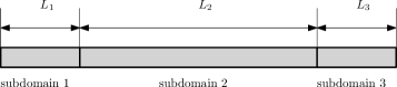
Figure 7. One-dimensional problem: The computational domain is divided into three subdomains of lengths $L_{1}=0.1$, $L_{2}=0.8$, and $L_{3}=0.1$. Two-node linear finite elements are used in all the subdomains. The source is unity in the entire domain (i.e., $f(\mathrm{x},t)=1$). It should be noted that there will be boundary layers for the chosen parameters. In order to adequately capture these boundary layers, we shall employ very fine meshes in subdomains one and three.

The domain is decomposed into three subdomains, as shown in Figure 7. Subdomains 1 and 3 are the regions in which the boundary layers will appear. Note that these subdomains are meshed using much finer elements than subdomain 2. For time-integration variables, see tables 3 and 4. The numerical results obtained using the proposed multi-time-step coupling methods are shown in Figures 8 and 9. Results are in good agreement with the exact solution, and the boundary layers are captured accurately by the proposed coupling methods. The drifts in concentrations and rate variables are plotted in figures 10 and 11. This numerical experiment illustrates the following attractive features of the proposed coupling methods:

1. The system time-step can be much larger than subdomain time-steps.

2. For fixed subdomain time-steps, smaller system time-step will result in better accuracy.

3. Under the coupling method based on the Baumgarte stabilization and fixed subdomain time-steps, decreasing system time-step and/or increasing the Baumgarte stabilization parameter will result in improved accuracy.

4. Utilizing smaller time-steps in individual subdomains improves the accuracy of results in the respective subdomain.

Table 3. One-dimensional problem: Time-integration parameters for the $d$-continuity method.

Case	$\Delta t$	$\Delta t_{1}$	$\Delta t_{2}$	$\Delta t_{3}$	$\vartheta_{1}$	$\vartheta_{2}$	$\vartheta_{3}$
1	0.25	0.05	0.25	0.05	1/2	1	1/2
2	0.25	0.05	0.01	0.05	1/2	1	1/2
3	0.1	0.1	0.1	0.1	1/2	1/2	1/2

Table 4. One-dimensional problem: Time-integration parameters for the Baumgarte stabilization method.

Case	$\Delta t$	$\alpha$	$\Delta t_{1}$	$\Delta t_{2}$	$\Delta t_{3}$	$\vartheta_{1}$	$\vartheta_{2}$	$\vartheta_{3}$
1	0.25	1	0.125	0.25	0.125	1/2	0	1/2
2	0.25	5	0.125	0.05	0.125	1/2	0	1/2
3	0.25	5	0.00125	0.25	0.00125	0	1	0
4	0.25	1	0.0025	0.25	0.0025	0	1	0
5	0.1	1	0.1	0.1	0.1	1/2	1/2	1/2

5.3. Two-dimensional problem

A transient version of the well-known problem proposed by Hemker [Hemker, 1996] will be considered. The governing equations take the following form:

$$\frac{\partial\mathrm{c}}{\partial t}+\frac{\partial\mathrm{c}}{\partial\mathrm{x}}-\varepsilon\mathrm{div}\left[\mathrm{grad}[\mathrm{c}]\right]=0\quad \mathrm{in}\;\Omega$$ (5.4a)

$$\mathrm{c}(\mathrm{x},\mathrm{y},t)=1\quad \mathrm{on}\;\Gamma^{\mathrm{D}}_{1}$$ (5.4b)

$$\mathrm{c}(\mathrm{x},\mathrm{y},t)=0\quad \mathrm{on}\;\Gamma^{\mathrm{D}}_{2}$$ (5.4c)

$$- \varepsilon\mathrm{grad}[\mathrm{c}]\cdot\widehat{\mathbf{n}}(\mathbf{x})=0\quad \mathrm{on}\;\Gamma^{\mathrm{N}}$$ (5.4d)

$$\mathrm{c}(\mathrm{x},\mathrm{y},t=0)=0\quad \mathrm{in}\;\Omega$$ (5.4e)

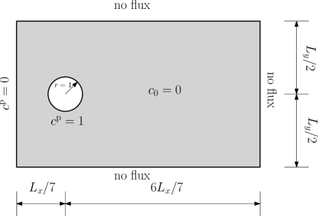
Figure 12. Two-dimensional transient Hemker problem: The dimensions of the computational domain are taken as $L_{x}=14$ and $L_{y}=8$. A circular hole is centered at the origin, and has a radius of unity. Concentration is unity on the circumference of the circle, and zero along the left side of the domain. No-flux boundary condition is enforced on the rest of the boundary. The prescribed initial condition is zero.

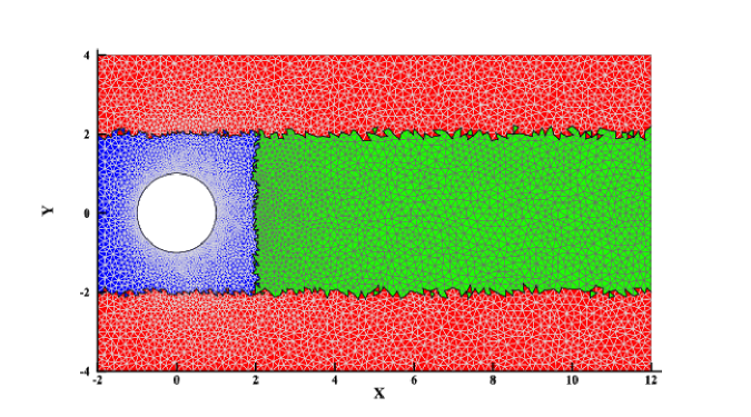
Figure 13. Two-dimensional transient Hemker problem: This figure shows the computational mesh, and the decomposition of the domain into subdomains. The computational domain is meshed using 11512 triangular finite elements using GMSH [Geuzaine and Remacle, 2009], and is partitioned into three subdomains. The first subdomain is indicated in blue color, the second subdomain is in green color, and the third subdomain is in red color. (See the online version of the paper for a color picture.)

Computational domain, mesh, and domain decomposition are shown in Figures 12 and 13. In this problem, the advection velocity is $\mathbf{v}=(1,0)$, and $\varepsilon=0.01$. The problem at hand is a singularly perturbed equation and is known to exhibit both boundary and interior layers. Furthermore, the standard Galerkin formulation is known to produce spurious oscillations for small values of $\varepsilon$ [Gresho and Sani, 2000].

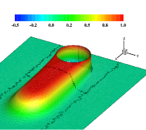
(b) Baumgarte stabilization

Figure 14. Two-dimensional transient Hemker problem: The value of concentrations is shown on the domain of interest at $t=5$. In this particular example, Galerkin weak formulation is employed. In figure (a), $d$-continuity method is employed to enforce continuity at the subdomain interface. The computational domain is partitioned into three subdomains. Figure (b) shows the results when Baumgarte stabilization is employed to enforce continuity at the interface. Spurious oscillations due to semi-discrete Galerkin method can be seen in near the circle. The minimum value of concentrations seen in these examples is -0.439, which is significant compared to the maximum, which is unity. The values of numerical time-integration parameters are given in Table 5.

The numerical results obtained using the Galerkin weak formulation are shown in Figure 14. As expected, spurious oscillations occur at the vicinity of the circle. The minimum value observed in both cases is -0.439. The spurious oscillations and the violation of the non-negative constraint is because of using the Galerkin weak formulation, and is not due to the use of proposed multi-time-step coupling methods. To corroborate this claim, Figure 15 shows the results where tailored weak formulations are employed in different subdomains. The GLS formulation is used in subdomain 1, the SUPG formulation is employed in subdomain 2, and the Galerkin formulation in subdomain 3. There are no spurious oscillations and the minimum value observed is -0.062. In Figure 16, the $\infty$-norm of drift of concentrations from compatibility constraints is shown. There is no noticeable drift and in the case of Baumgarte stabilization method, the the drifts are controlled. Time integration parameters are given in tables 5 and 6. This example demonstrates choice of disparate time-steps, and different numerical formulations in different spatial regions of the computational domain.

Table 5. Two-dimensional transient Hemker problem: Time-integration parameters for results using the standard Galerkin method.

Compatibility condition	$\Delta t$	$\alpha$	$\Delta t_{1}$	$\Delta t_{2}$	$\Delta t_{3}$	$\vartheta_{1}$	$\vartheta_{2}$	$\vartheta_{3}$
$d$-continuity method	0.1		0.001	0.01	0.1	1/2	1	1
Baumgarte stabilization	0.2	1	0.01	0.05	0.02	1/2	1	0

Table 6. Two-dimensional transient Hemker problem: Time-integration parameters for results using the GLS-SUPG-Galerkin formulations.

Compatibility condition	$\Delta t$	$\alpha$	$\Delta t_{1}$	$\Delta t_{2}$	$\Delta t_{3}$	$\vartheta_{1}$	$\vartheta_{2}$	$\vartheta_{3}$
$d$-continuity method	0.2		0.001	0.005	0.2	1/2	1	1
Baumgarte stabilization	0.2	1	0.001	0.005	0.02	1	1/2	0

6. MULTI-TIME-STEP TRANSIENT ANALYSIS OF A TRANSPORT-CONTROLLED BIMOLECULAR REACTION

In this section, we shall apply the proposed multi-time-step coupling methods to a transport-controlled bimolecular reaction. This problem is of tremendous practical importance in areas such as transverse mixing-limited chemical reactions in groundwater and aquifers, and mixing-controlled bioreactive transport in heterogeneous porous media arising in bioremediation. We shall now document the most important equations of the mathematical model. A more detailed discussion about the model can be found in [Nakshatrala et al., 2013], which however did not address multi-time-step coupling methods.

6.1. Mathematical model

Consider the following irreversible chemical reaction:

$$n_{A}A+n_{B}B\rightarrow n_{C}C$$ (6.1)

where $A$, $B$ and $C$ are the chemical species participating in the reaction, and $n_{A}$, $n_{B}$ and $n_{C}$ are their respective (positive) stoichiometry coefficients. The fate of the reactants and the product are governed by coupled system of transient advection-diffusion-reaction equations. We shall assume the part of the boundary on which the Dirichlet boundary condition is enforced to be the same for the reactants and the product. Likewise is assumed for the Neumann boundary conditions. One can then find two invariants that are unaffected by the underlying reaction, which can be obtained via the following linear transformation:

$$\mathrm{c}_{F}:=\mathrm{c}_{A}+\left(\frac{n_{A}}{n_{C}}\right)\mathrm{c}_{C}$$ (6.2a)

$$\mathrm{c}_{G}:=\mathrm{c}_{B}+\left(\frac{n_{B}}{n_{C}}\right)\mathrm{c}_{C}$$ (6.2b)

The evolution of these invariants is given by the following uncoupled transient advection-diffusion equations:

$$\frac{\partial\mathrm{c}_{i}}{\partial t}+\mathrm{div}\left[\mathbf{v}\mathrm{c}_{i}-\mathbf{D}(\mathbf{x})\mathrm{grad}[\mathrm{c}_{i}]\right]=f_{i}(\mathbf{x},t)\quad \mathrm{in}\;\Omega\times\mathcal{I}$$ (6.3a)

$$\mathrm{c}_{i}(\mathbf{x},t)=\mathrm{c}_{i}^{\mathrm{p}}(\mathbf{x},t):=\mathrm{c}_{j}^{\mathrm{p}}(\mathbf{x},t)+\left(\frac{n_{j}}{n_{C}}\right)\mathrm{c}_{C}^{\mathrm{p}}(\mathbf{x},t)\quad \mathrm{on}\;\Gamma^{\mathrm{D}}\times\mathcal{I}$$ (6.3b)

$$- \widehat{\mathbf{n}}(\mathbf{x})\cdot\mathbf{D}(\mathbf{x})\mathrm{grad}[\mathrm{c}_{i}]=h_{i}^{\mathrm{p}}(\mathbf{x},t):=h_{j}^{\mathrm{p}}(\mathbf{x},t)+\left(\frac{n_{j}}{n_{C}}\right)h_{C}^{\mathrm{p}}(\mathbf{x},t)\quad \mathrm{on}\;\Gamma^{\mathrm{N}}\times\mathcal{I}$$ (6.3c)

$$\mathrm{c}_{i}(\mathbf{x},t=0)=\mathrm{c}_{i}^{0}(\mathbf{x}):=\mathrm{c}_{j}^{0}(\mathbf{x})+\left(\frac{n_{j}}{n_{C}}\right)\mathrm{c}_{C}^{0}(\mathbf{x})\quad \mathrm{in}\;\Omega$$ (6.3d)

where $i=F$ or $G$. We shall restrict to fast bimolecular reactions. That is, the time-scale of the chemical reaction is much smaller than the time-scale of the transport processes. For such situations, one can assume that the chemical species $A$ and $B$ cannot coexist at a spatial point and for a given instance of time. This implies that the concentrations of the reactants and the product can be obtained from the concentrations of the invariants through algebraic manipulations. To wit,

$$\mathrm{c}_{A}\left(\mathbf{x},t\right)=\mathrm{max}\left\{\mathrm{c}_{F}\left(\mathbf{x},t\right)-\left(\frac{n_{A}}{n_{B}}\right)\mathrm{c}_{G}\left(\mathbf{x},t\right),0\right\}$$ (6.4a)

$$\mathrm{c}_{B}\left(\mathbf{x},t\right)=\left(\frac{n_{B}}{n_{A}}\right)\mathrm{max}\left\{-\mathrm{c}_{F}\left(\mathbf{x},t\right)+\left(\frac{n_{A}}{n_{B}}\right)\mathrm{c}_{G}\left(\mathbf{x},t\right),0\right\}$$ (6.4b)

$$\mathrm{c}_{C}\left(\mathbf{x},t\right)=\left(\frac{n_{C}}{n_{A}}\right)\left(\mathrm{c}_{F}\left(\mathbf{x},t\right)-\mathrm{c}_{A}\left(\mathbf{x},t\right)\right)$$ (6.4c)

Note that the solution procedure is still nonlinear, as the $\mathrm{max}\{\cdot,\cdot\}$ operator is nonlinear.

We shall employ the proposed multi-time-step computational framework to solve equations (6.3a)–(6.3d) to obtain concentrations of the invariants. Using the calculated values, we then find the concentrations for the reactants and the product using equations (6.4a)–(6.4c). The Galerkin formulation is employed in all subdomains. The negative values for the concentration are clipped at every subdomain time-step in the numerical simulations.

6.2. Numerical results for a diffusion-controlled bimolecular reaction

Consider a reaction chamber with $L_{x}=L_{y}=1$, as shown in Figure 17. The computational domain is meshed using 5442 four-node quadrilateral elements. As shown in this figure, the domain is decomposed into four non-contiguous subdomains using METIS [Karypis and Kumar, 1999]. The diffusivity tensor is taken as follows:

$$\mathbf{D}\left(\mathrm{x},\mathrm{y}\right)=\left[\begin{array}[]{c c}\gamma\mathrm{x}^{2}+\mathrm{y}^{2}&-\left(1-\gamma\right)\mathrm{x}\mathrm{y}\\ -\left(1-\gamma\right)\mathrm{x}\mathrm{y}&\mathrm{x}^{2}+\gamma\mathrm{y}^{2}\end{array}\right]$$ (6.7)

where $\gamma=0.001$. Baumgarte stabilization is employed to enforce compatibility along the subdomain interfaces with $\alpha=100$. Implicit Euler method is employed in subdomains 1 and 3, and midpoint rule is employed in subdomains 2 and 4. The system time-step is taken as $\Delta t=10^{-3}$, and the subdomain time-steps are taken as $\Delta t_{1}=\Delta t_{3}=5\times 10^{-4}$, and $\Delta t_{2}=\Delta t_{4}=10^{-3}$.

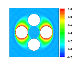
(b) Concentration of invariant $F$ at $t=0.1$.

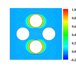
(c) Concentration of invariant $G$ at $t=0.01$.

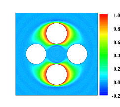
(d) Concentration of invariant $G$ at $t=0.1$.

Figure 18. Diffusion-controlled fast bimolecular reaction: This figure shows the concentrations of the invariants $F$ and $G$ at $t=0.01$ and $t=0.1$.

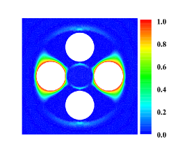
(b) Concentration of reactant $A$ at $t=0.1$.

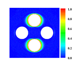
(c) Concentration of reactant $B$ at $t=0.01$.

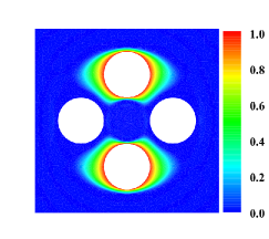
(d) Concentration of reactant $B$ at $t=0.1$.

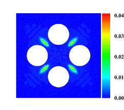
(e) Concentration of product $C$ at $t=0.01$.

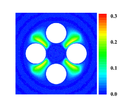
(f) Concentration of product $C$ at $t=0.1$.

Figure 19. Diffusion-controlled fast bimolecular reaction:  Concentrations of the reactants and the product are shown at $t=0.01$ and $t=0.1$.

Numerical results for the concentrations of the invariants, reactants and product are shown in Figures 18 and 19. As discussed earlier, Baumgarte stabilized coupling method can result in drift in the primary variable but it can be controlled using the stabilization parameter $\alpha$. Equation (4.31) can serve as a valuable tool assessing the overall behavior of drifts with respect to system time-step, and the Baumgarte stabilization parameter $\alpha$. Drifts for several choices of $\alpha$ and $\Delta t$ are shown in Figure 20. Note that equation (4.31) assumes no subcycling, and no mixed time-integration.

6.3. Numerical results for a fast bimolecular reaction with advection

Consider a reaction chamber with $L_{x}=4$ and $L_{y}=1$, as shown in Figure 21(a). The computational domain is meshed using three-node triangular elements, and METIS [Karypis and Kumar, 1999] is employed to decomposed the domain into four non-contiguous subdomains using , as shown in Figure 21(b). There are 4151 interface constraints to ensure continuity of concentration along the subdomain interface. The diffusivity tensor is taken as follows:

$$\mathbf{D}(\mathbf{x})=\alpha_{T}\|\mathbf{v}\|\mathbf{I}+\frac{\alpha_{L}-\alpha_{T}}{\|\mathbf{v}\|}\mathbf{v}\otimes\mathbf{v}$$ (6.8)

where $\mathbf{I}$ is the second-order identity tensor, $\otimes$ is the tensor product, $\|\cdot\|$ is the 2-norm, $\mathbf{v}(\mathbf{x})$ is the velocity, and $\alpha_{L}$ and $\alpha_{T}$ are, respectively, the longitudinal and transverse diffusivities. This form of diffusivity tensor is commonly employed in subsurface hydrology [Pinder and Celia, 2006]. We define the velocity through the following stream function:

$$\psi(\mathrm{x},\mathrm{y})=-\mathrm{y}-\sum_{k=1}^{3}A_{k}\mathrm{cos}\left(\frac{p_{k}\pi\mathrm{x}}{L_{x}}-\frac{\pi}{2}\right)\mathrm{sin}\left(\frac{q_{k}\pi\mathrm{y}}{L_{y}}\right)$$ (6.9)

The components of the advection velocity can then be calculated as follows:

$$\mathrm{v}_{x}(\mathrm{x},\mathrm{y})=-\frac{\partial\psi}{\partial\mathrm{y}},\quad\mathrm{v}_{y}(\mathrm{x},\mathrm{y})=+\frac{\partial\psi}{\partial\mathrm{x}}$$ (6.10)

The following parameters are used in the numerical simulation:

$$p_{1}=4,\;p_{2}=5,\;p_{3}=10,\;q_{1}=1,\;q_{2}=5,\;q_{3}=10,\;A_{1}=0.08,\;A_{2}=0.02,\;A_{3}=0.01$$ (6.11)

The diffusivities are taken as $\alpha_{L}=1$ and $\alpha_{T}=10^{-4}$, and the prescribed concentrations on the boundary are taken as $c_{A}^{\mathrm{p}}=1.0$ and $c_{B}^{\mathrm{p}}=1.5$.

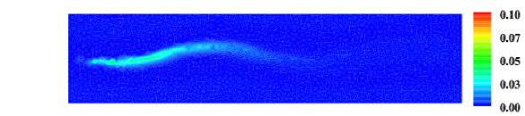
(a) Concentration of the product $C$ at $t=0.5.$

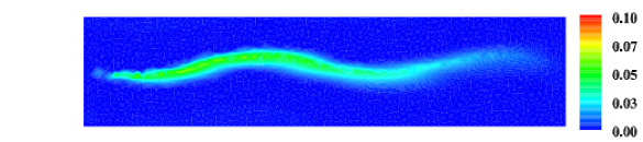
(b) Concentration of the product $C$ at $t=1.5.$

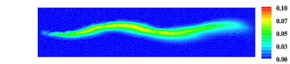
(c) Concentration of the product $C$ at $t=4.0.$

Figure 22. Fast bimolecular reaction with advection: This figure shows the concentration of the product $C$ at various instances of time obtained using the proposed $d$-continuity multi-time-step coupling method. The system time-step is taken to be $\Delta t=0.1$, and the subdomain time-steps are $\Delta t_{1}=0.01$, $\Delta t_{2}=0.05$, $\Delta t_{3}=0.01$ and $\Delta t_{4}=0.05$. Implicit Euler method is employed in subdomains 1 and 3 (i.e., $\vartheta_{1}=\vartheta_{3}=1$), and the midpoint rule is employed in subdomains 2 and 4 (i.e., $\vartheta_{2}=\vartheta_{4}=1/2$). As one can see from the figure, there is no drift along the subdomain interface, and the proposed coupling method performed well.

The numerical results for the concentration of the product at various time levels obtained using the $d$-continuity coupling method are shown in Figure 22, and there is no drift along the subdomain interface, which is expected under the proposed $d$-continuity method.

The above numerical examples clearly demonstrate that the proposed multi-time-step coupling methods can handle any decomposition of the computational domain: either the subdomains are contiguous or non-contiguous; whether the decomposition is based on the physics of the problem or based on numerical performance; or whether the decomposition is done manually by the user or obtained from a graph-partitioning software package.

7. CONCLUDING REMARKS

We presented a stable multi-time-step computational framework for transient advective-diffusive-reactive systems. The computational domain can be divided into an arbitrary number of subdomains. Different time-stepping schemes under the trapezoidal family can be used in different subdomains. Different time-steps and different numerical formulations can be employed in different subdomains. Unlike many of the prior works on multi-time-step methods (e.g., staggered schemes proposed in [Piperno, 1997]), no preferential treatment is given to the subdomain with the largest subdomain time-step, and thereby eliminating the associated subdomain-dependent solutions.

Under the framework, we proposed two different monolithic coupling methods, which differ in the way compatibility conditions are enforced along the subdomain interface. Under the first method (i.e., $d$-continuity method), the continuity of the primary variable is enforced along the subdomain interface at every system time-step. An attractive feature of the $d$-continuity method is that, by construction, there is no drift in the primary variable along the subdomain interface. However, one cannot couple explicit and implicit schemes under the $d$-continuity method. But this method has good stability characteristics. The second method is based on an extension of the classical Baumgarte stabilization [Baumgarte, 1972; Nakshatrala et al., 2009] to first-order transient systems. Under this method one can couple explicit and implicit schemes. However, there can be drift in the primary variable along the subdomain interface. But this drift is bounded and small, which we have shown both theoretically and numerically. The other salient features of the proposed coupling methods are as follows: There is no limitation on the number of subdomains or on the subcycling ratios $\eta_{i}$. Since no preference is given to any subdomain, the numerical solutions under the proposed coupling methods will not be affected by the way the computational domain is decomposed into subdomains. This is also evident from the numerical results presented in this paper. The coupling methods are shown to be stable, which has been illustrated both mathematically and numerically.

Based on the above discussion, we shall make the following two recommendations for a multi-time-step analysis of first-order transient systems:

1. If it is not needed to couple explicit/implicit time integrators, but one just wants to use different time-steps and different numerical formulations in different regions, then it is recommended to use the proposed $d$-continuity method. If one wants to couple explicit and implicit schemes, then one has to use the proposed coupling method based on Baumgarte stabilization.

2. Accuracy can be improved by decreasing the system time-step.

A possible research work can be towards the implementation of the proposed multi-time-step coupling methods in a parallel computing environment and on graphical processing units (GPUs).

APPENDIX: A COMPACT NOTATION FOR COMPUTER IMPLEMENTATION

Herein, we present a compact matrix form for the proposed coupling methods. In fact, we present in a more general setting by considering nonlinear first-order transient DAEs of the following form:

$$\boldsymbol{M}_{i}\dot{\boldsymbol{c}}_{i}\left(t\right)=\boldsymbol{h}_{i}\left(\boldsymbol{c}_{i}\left(t\right),t\right)+\boldsymbol{C}_{i}^{\mathrm{T}}\boldsymbol{\lambda}\left(t\right)\quad\forall i$$ (7.1)

$$\sum_{i=1}^{\mathcal{S}}\boldsymbol{C}_{i}\boldsymbol{c}_{i}\left(t\right)=\boldsymbol{0}$$ (7.2)

We will employ a Newton-Raphson-based approach to solve the given system of equation. Other methods of solving nonlinear equations (e.g., Picard method) can also be utilized. However for simplicity of the presentation, we shall ignore further details on solution techniques for solving nonlinear equations.

The resulting system of equations will have to be solved in iterations until some suitable convergence condition is met. Let us denote the differentiation operator with respect to $\boldsymbol{u}$ by $\mathrm{D}$ (i.e., $\mathrm{D}:=\partial/\partial\boldsymbol{u}$). Let $\Box^{\left(n+(j+1)/\eta_{i}\right)}_{i,\nu}$ denote the nodal values of $\Box$ in the $i$-th subdomain, at time-level $n+\frac{j+1}{\eta_{i}}$, and after $\nu$ iterations. The following notation will be useful:

$$\boldsymbol{h}_{i,\nu}^{\left(n+\frac{j+1}{\eta_{i}}\right)}=\boldsymbol{h}_{i}\left(\boldsymbol{d}_{i,\nu}^{\left(n+\frac{j+1}{\eta_{i}}\right)},t^{\left(n+\frac{j+1}{\eta_{i}}\right)}\right)$$ (7.3)

$$\mathrm{D}\boldsymbol{h}_{i,\nu}^{\left(n+\frac{j+1}{\eta_{i}}\right)}=\mathrm{D}\boldsymbol{h}_{i}\left(\boldsymbol{d}_{i,\nu}^{\left(n+\frac{j+1}{\eta_{i}}\right)},t^{\left(n+\frac{j+1}{\eta_{i}}\right)}\right)$$ (7.4)

The unknowns at all subdomain time-levels for the $i$-th subdomain and for a given Newton-Raphson iteration number $\nu$ can be grouped as follows:

$$\boldsymbol{X}_{i,\nu+1}^{\left(n+\frac{j}{\eta_{i}}\right)}=\left[\begin{array}[]{c}\boldsymbol{v}_{i,\nu+1}^{\left(n+\frac{j}{\eta_{i}}\right)}\\ \boldsymbol{d}_{i,\nu+1}^{\left(n+\frac{j}{\eta_{i}}\right)}\end{array}\right],\quad\mathbb{X}_{i,\nu+1}^{\left(n+1\right)}=\left[\begin{array}[]{c}\boldsymbol{X}_{i,\nu+1}^{\left(n+\frac{1}{\eta_{i}}\right)}\\ \boldsymbol{X}_{i,\nu+1}^{\left(n+\frac{2}{\eta_{i}}\right)}\\ \vdots\\ \boldsymbol{X}_{i,\nu+1}^{\left(n+1\right)}\end{array}\right],\quad\mathbb{X}_{\nu+1}^{\left(n+1\right)}=\left[\begin{array}[]{c}\mathbb{X}_{1,\nu+1}^{\left(n+1\right)}\\ \mathbb{X}_{2,\nu+1}^{\left(n+1\right)}\\ \vdots\\ \mathbb{X}_{\mathcal{S},\nu+1}^{\left(n+1\right)}\end{array}\right]$$ (7.15)

Using equation (7.3) and the trapezoidal time-stepping schemes, the following linearized matrices can be constructed:

$$\mathbb{L}_{i,\nu}^{\left(n+\frac{j+1}{\eta_{i}}\right)}=\left[\begin{array}[]{c c}\boldsymbol{M}_{i}&-\mathrm{D}\boldsymbol{h}_{i,\nu}^{\left(n+\frac{j+1}{\eta_{i}}\right)}\\ -\vartheta_{i}\Delta t_{i}\boldsymbol{I}_{i}&\boldsymbol{I}_{i}\end{array}\right],\quad\mathbb{R}_{i}=\left[\begin{array}[]{c c}\mathcal{O}_{i}&\mathcal{O}_{i}\\ \left(1-\vartheta_{i}\right)\Delta t_{i}\boldsymbol{I}_{i}&\boldsymbol{I}_{i}\end{array}\right],\quad\mathbb{C}_{i}=\left[\boldsymbol{C}_{i}\quad\mathrm{O}_{i}\right]$$ (7.20)

where $\mathcal{O}_{i}$ and $\boldsymbol{I}_{i}$ are, respectively, zero matrix and identity matrix of size $N_{i}\times N_{i}$, and the matrix $\mathrm{O}_{i}$ is a zero matrix of size $N_{\lambda}\times N_{i}$. The forcing function and the results from the previous iteration can be compactly assumed into the following vector:

$$\boldsymbol{F}_{i,\nu}^{\left(n+\frac{j+1}{\eta_{i}}\right)}=\left[\begin{array}[]{c}\boldsymbol{h}_{i,\nu}^{\left(n+\frac{j+1}{\eta_{i}}\right)}-\mathrm{D}\boldsymbol{h}_{i,\nu}^{\left(n+\frac{j+1}{\eta_{i}}\right)}\boldsymbol{d}_{i,\nu}^{\left(n+\frac{j+1}{\eta_{i}}\right)}\\ \boldsymbol{0}\end{array}\right]$$ (7.23)

Now, let the square matrices $\mathbb{A}_{i,\nu}$ and $\mathbb{A}_{\nu}$, and column vectors $\mathbb{F}_{\nu}^{\left(n+1\right)}$ and $\mathbb{F}_{\nu}^{\left(n+1\right)}$ be defined as below:

$$\mathbb{A}_{i,\nu}^{(n+1)}=\underbrace{\left[\begin{array}[]{c c c c}\mathbb{L}_{i,\nu}^{\left(n+\frac{1}{\eta_{i}}\right)}&&&\\ -\mathbb{R}_{i}&\mathbb{L}_{i,\nu}^{\left(n+\frac{2}{\eta_{i}}\right)}&&\\ &\ddots&\ddots&\\ &&-\mathbb{R}_{i}&\mathbb{L}_{i,\nu}^{\left(n+1\right)}\end{array}\right]}_{2\eta_{i}N_{i}},\quad\mathbb{A}_{\nu}^{(n+1)}=\left[\begin{array}[]{c c c c}\mathbb{A}_{1,\nu}^{(n+1)}&&&\\ &\mathbb{A}_{2,\nu}^{(n+1)}&&\\ &&\ddots&\\ &&&\mathbb{A}_{\mathcal{S},\nu}^{(n+1)}\end{array}\right]$$ (7.32)

$$\mathbb{F}_{i,\nu}^{\left(n+1\right)}=\left[\begin{array}[]{c}\boldsymbol{F}_{i,\nu}^{\left(n+\frac{1}{\eta_{i}}\right)}+\mathbb{R}_{i}\boldsymbol{X}_{i}^{\left(n\right)}+\mathbb{C}_{i}^{\mathrm{T}}\boldsymbol{\lambda}^{\left(n\right)}\\ \boldsymbol{F}_{i,\nu}^{\left(n+\frac{2}{\eta_{i}}\right)}+\mathbb{C}_{i}^{\mathrm{T}}\boldsymbol{\lambda}^{\left(n\right)}\\ \vdots\\ \boldsymbol{F}_{i,\nu}^{\left(n+1\right)}+\mathbb{C}_{i}^{\mathrm{T}}\boldsymbol{\lambda}^{\left(n\right)}\end{array}\right],\quad\mathbb{F}_{\nu}^{\left(n+1\right)}=\left[\begin{array}[]{c}\mathbb{F}_{1,\nu}^{\left(n+1\right)}\\ \mathbb{F}_{2,\nu}^{\left(n+1\right)}\\ \vdots\\ \mathbb{F}_{\mathcal{S},\nu}^{\left(n+1\right)}\end{array}\right]$$ (7.41)

Enforcing the algebraic constraints can be done using the following matrices:

$$\mathbb{B}_{i} =\underbrace{\left[\mathrm{O}_{i}\quad\mathrm{O}_{i}\quad\ldots\quad\overbrace{\mathrm{O}_{i}\quad\boldsymbol{C}_{i}}^{2N_{i}}\right]}_{2\eta_{i}N_{i}}\quad\mbox{for $d$-continuity method}$$ (7.42)

$$\mathbb{B}_{i} =\underbrace{\left[\mathrm{O}_{i}\quad\mathrm{O}_{i}\quad\ldots\quad\overbrace{\boldsymbol{C}_{i}\quad\frac{\alpha}{\Delta t}\boldsymbol{C}_{i}}^{2N_{i}}\right]}_{2\eta_{i}N_{i}}\quad\mbox{for Baumgarte stabilization method}$$ (7.43)

Using the notation above, one can then construct the following augmented matrix:

$$\mathbb{B}=\left[\mathbb{B}_{1}\quad\mathbb{B}_{2}\quad\ldots\quad\mathbb{B}_{\mathcal{S}}\right]$$ (7.44)

The algebraic constraint (for both $d$-continuity and Baumgarte stabilization) can be compactly written as follows:

$$\mathbb{B}\mathbb{X}_{\nu+1}^{\left(n+1\right)}=\boldsymbol{0}$$ (7.45)

We define the matrix $\mathbb{C}$ as below:

$$\mathbb{C}=\underbrace{\left[\quad-\frac{1}{\eta_{1}}\mathbb{C}_{1}\quad-\frac{2}{\eta_{1}}\mathbb{C}_{1}\quad\ldots\quad-\mathbb{C}_{1}\quad|\quad\ldots\quad|\quad-\frac{1}{\eta_{\mathcal{S}}}\mathbb{C}_{\mathcal{S}}\quad-\frac{2}{\eta_{\mathcal{\mathcal{S}}}}\mathbb{C}_{\mathcal{S}}\quad\ldots\quad-\mathbb{C}_{\mathcal{S}}\quad\right]}_{\sum_{i=1}^{\mathcal{S}}2\eta_{i}N_{i}}$$ (7.46)

Finally, time marching can be performed by solving the following equation:

$$\left[\begin{array}[]{c | c}\mathbb{A}_{\nu}^{(n+1)}&\mathbb{C}^{\mathrm{T}}\\ \hline\cr\mathbb{B}&\mathbb{O}\end{array}\right]\left[\begin{array}[]{c}\mathbb{X}_{\nu+1}^{\left(n+1\right)}\\ \hline\cr\boldsymbol{\lambda}_{\nu+1}^{\left(n+1\right)}-\boldsymbol{\lambda}^{\left(n\right)}\end{array}\right]=\left[\begin{array}[]{c}\mathbb{F}_{\nu}^{\left(n+1\right)}\\ \hline\cr\boldsymbol{0}\end{array}\right]$$ (7.53)

which gives the values of the nodal concentrations and the corresponding rates within a Newton-Raphson iteration for all subdomains and at all subdomain time-levels within a system time-step. The solution procedure is outlined in Algorithm 1.

Algorithm 1 Multi-time-step transient analysis using the proposed coupling methods.

1:  Generate subdomain specific matrices and vectors $\boldsymbol{M}_{i}$, $\boldsymbol{C}_{i}$, and $\boldsymbol{h}_{i}$

2:  Read time integration parameters: $\Delta t$, $\Delta t_{i}$ ($i=1,\cdots,\mathcal{S}$), and $\alpha$ (in the case of Baumgarte stabilization)

2:  Time integration parameters should satisfy the criteria given in Theorems 2 and 4

3:  Read the initial values $\boldsymbol{d}_{i}^{(0)}$ ($i=1,\cdots,\mathcal{S}$)

4:  Calculate the initial values for the Lagrange multipliers, $\boldsymbol{\lambda}^{(0)}$, by solving the following system: $\left(\sum_{i=1}^{\mathcal{S}}\boldsymbol{C}_{i}\boldsymbol{M}_{i}^{-1}\boldsymbol{C}_{i}^{\mathrm{T}}\right)\boldsymbol{\lambda}^{(0)}=-\sum_{i=1}^{\mathcal{S}}\boldsymbol{C}_{i}\boldsymbol{M}_{i}^{-1}\boldsymbol{h}_{i}\left(\boldsymbol{d}_{i}^{(0)},t=0\right)$

5:  Calculate the initial values of the rate variables: $\boldsymbol{M}_{i}\boldsymbol{v}_{i}^{(0)}=\boldsymbol{h}_{i}\left(\boldsymbol{d}_{i}^{(0)},t=0\right)+\boldsymbol{C}_{i}^{\mathrm{T}}\boldsymbol{\lambda}^{(0)}\quad\forall i=1,...,\mathcal{S}$

6:  Specify some convergence criteria (e.g., maximum number of iterations, maximum tolerance for concentrations, rate variables, or the Lagrange multipliers)

7:  for $n=1,\cdots,\mathcal{N}$ do

8:     Initiate the iteration counter: $\nu\leftarrow 0$

9:     Assign values for $\boldsymbol{d}_{i,0}^{(n+j/\eta_{i})}$ (for $i=1,\cdots,\mathcal{S}$ and $j=1,\cdots,\eta_{i}$) {a consistent initial guess for the nodal concentrations}

10:     repeat

11:        Set $\nu\leftarrow\nu+1$

12:        Initiate/update $\mathbb{A}_{\nu-1}^{(n)}$ according to equation (7.32)

13:        Initiate/update $\mathbb{F}_{\nu-1}^{(n)}$ according to equation (7.32)

14:        Solve for $\mathbb{X}_{\nu}^{(n)}$ and $\boldsymbol{\lambda}_{\nu}^{(n)}$ using equation (7.53)

15:     until convergence criteria are met

16:  end for

\psfrag{1}{$\omega_{1}$}\psfrag{2}{$\omega_{2}$}\psfrag{3}{$\omega_{3}$}\psfrag{...}{$\cdots$}\psfrag{S}{$\omega_{\mathcal{S}}$}\psfrag{omega}{$\Omega$}\psfrag{i}{Interface interaction}\psfrag{l}{$\boldsymbol{\lambda}$}\includegraphics[scale={0.75}]{dual_schur.eps}

Figure 1. A pictorial description of computational domain and its decomposition into subdomains, subdomain interface, and interface interactions (i.e., Lagrange multipliers).

\psfrag{1}{Subdomain 1}\psfrag{2}{Subdomain 2}\psfrag{S}{Subdomain $\mathcal{S}$}\psfrag{ex}{Information exchange}\psfrag{system}{System time-step $\Delta t$}\psfrag{tn}{$t_{n}$}\psfrag{tn+1}{$t_{n+1}$}\psfrag{dt1}{$\Delta t_{1}$}\psfrag{dt2}{$\Delta t_{2}$}\psfrag{dtS}{$\Delta t_{\mathcal{S}}$}\psfrag{vdot}{$\vdots$}\psfrag{en}{enforcement of compatibility conditions at system time-levels}\includegraphics[scale={0.8}]{multi-time-step.eps}

Figure 2. A pictorial description of time levels ($t_{n}$), system time-step $(\Delta t)$, subdomain time-step $(\Delta t_{i})$, and subcycling. By subcycling in the $i$-th subdomain we mean that $\Delta t_{i}<\Delta t$.

\psfrag{m1}{$m_{1}$}\psfrag{m2}{$m_{2}$}\psfrag{f1}{$f_{1}$}\psfrag{f2}{$f_{2}$}\psfrag{k1}{$k_{1}$}\psfrag{k2}{$k_{2}$}\psfrag{l1}{$\lambda$}\psfrag{l2}{$-\lambda$}\includegraphics[scale={0.8}]{SDOF_problem.eps}

Figure 3. Split degree-of-freedom problem: A pictorial description.

\psfrag{time}{time}\psfrag{cons}{concentration}\psfrag{L}{$\lambda$}\psfrag{drift}{$d_{\mathrm{drift}}^{(n)}$}\psfrag{v_drift}{$v_{\mathrm{drift}}^{(n)}$}\psfrag{rate}{rate variable}\psfrag{exact}{exact solution}\psfrag{s1_1}{subdomain 1; case 1}\psfrag{s1_2}{subdomain 2; case 1}\psfrag{s2_1}{subdomain 1; case 2}\psfrag{s2_2}{subdomain 2; case 2}\psfrag{s3_1}{subdomain 1; case 3}\psfrag{s3_2}{subdomain 2; case 3}\psfrag{s1}{Case 1}\psfrag{s2}{Case 2}\psfrag{s3}{Case 3}\includegraphics[scale={0.3},clip]{SDOF_d_cons.eps}

\psfrag{time}{time}\psfrag{cons}{concentration}\psfrag{L}{$\lambda$}\psfrag{drift}{$d_{\mathrm{drift}}^{(n)}$}\psfrag{v_drift}{$v_{\mathrm{drift}}^{(n)}$}\psfrag{rate}{rate variable}\psfrag{exact}{exact solution}\psfrag{s1_1}{subdomain 1; case 1}\psfrag{s1_2}{subdomain 2; case 1}\psfrag{s2_1}{subdomain 1; case 2}\psfrag{s2_2}{subdomain 2; case 2}\psfrag{s3_1}{subdomain 1; case 3}\psfrag{s3_2}{subdomain 2; case 3}\psfrag{s1}{Case 1}\psfrag{s2}{Case 2}\psfrag{s3}{Case 3}\includegraphics[scale={0.3},clip]{SDOF_d_rate.eps}

\psfrag{time}{time}\psfrag{cons}{concentration}\psfrag{L}{$\lambda$}\psfrag{drift}{$d_{\mathrm{drift}}^{(n)}$}\psfrag{v_drift}{$v_{\mathrm{drift}}^{(n)}$}\psfrag{rate}{rate variable}\psfrag{exact}{exact solution}\psfrag{s1_1}{subdomain 1; case 1}\psfrag{s1_2}{subdomain 2; case 1}\psfrag{s2_1}{subdomain 1; case 2}\psfrag{s2_2}{subdomain 2; case 2}\psfrag{s3_1}{subdomain 1; case 3}\psfrag{s3_2}{subdomain 2; case 3}\psfrag{s1}{Case 1}\psfrag{s2}{Case 2}\psfrag{s3}{Case 3}\includegraphics[scale={0.3},clip]{SDOF_d_lambda.eps}

\psfrag{time}{time}\psfrag{cons}{concentration}\psfrag{L}{$\lambda$}\psfrag{drift}{$d_{\mathrm{drift}}^{(n)}$}\psfrag{v_drift}{$v_{\mathrm{drift}}^{(n)}$}\psfrag{rate}{rate variable}\psfrag{exact}{exact solution}\psfrag{s1_1}{subdomain 1; case 1}\psfrag{s1_2}{subdomain 2; case 1}\psfrag{s2_1}{subdomain 1; case 2}\psfrag{s2_2}{subdomain 2; case 2}\psfrag{s3_1}{subdomain 1; case 3}\psfrag{s3_2}{subdomain 2; case 3}\psfrag{s1}{Case 1}\psfrag{s2}{Case 2}\psfrag{s3}{Case 3}\includegraphics[scale={0.3},clip]{SDOF_d_drift.eps}

\psfrag{time}{time}\psfrag{cons}{concentration}\psfrag{L}{$\lambda$}\psfrag{drift}{$d_{\mathrm{drift}}^{(n)}$}\psfrag{v_drift}{$v_{\mathrm{drift}}^{(n)}$}\psfrag{rate}{rate variable}\psfrag{exact}{exact solution}\psfrag{s1_1}{subdomain 1; case 1}\psfrag{s1_2}{subdomain 2; case 1}\psfrag{s2_1}{subdomain 1; case 2}\psfrag{s2_2}{subdomain 2; case 2}\psfrag{s3_1}{subdomain 1; case 3}\psfrag{s3_2}{subdomain 2; case 3}\psfrag{s1}{Case 1}\psfrag{s2}{Case 2}\psfrag{s3}{Case 3}\includegraphics[scale={0.3},clip]{SDOF_d_v_drift.eps}

Figure 4. Split degree-of-freedom problem: We have employed the multi-time-step coupling method based on $d$-continuity method. The values of concentrations, rate variables, Lagrange multipliers, and drifts are compared with their respective exact solutions. It can be seen that the numerical results obtained using the proposed coupling method based on $d$-continuity method show very good compatibility with the exact solution. For values of time-integration parameters see Table 1. Values for the time-integration parameters are given in Table 1.

\psfrag{time}{time}\psfrag{cons}{concentration}\psfrag{L}{$\lambda$}\psfrag{rate}{rate variable}\psfrag{drift}{$d_{\mathrm{drift}}^{(n)}$}\psfrag{v_drift}{$v_{\mathrm{drift}}^{(n)}$}\psfrag{exact}{exact solution}\psfrag{s1_1}{subdomain 1; case 1}\psfrag{s1_2}{subdomain 2; case 1}\psfrag{s2_1}{subdomain 1; case 2}\psfrag{s2_2}{subdomain 2; case 2}\psfrag{s3_1}{subdomain 1; case 3}\psfrag{s3_2}{subdomain 2; case 3}\psfrag{s1}{Case 1}\psfrag{s2}{Case 2}\psfrag{s3}{Case 3}\includegraphics[scale={0.3},clip]{SDOF_Baumgarte_cons.eps}

\psfrag{time}{time}\psfrag{cons}{concentration}\psfrag{L}{$\lambda$}\psfrag{rate}{rate variable}\psfrag{drift}{$d_{\mathrm{drift}}^{(n)}$}\psfrag{v_drift}{$v_{\mathrm{drift}}^{(n)}$}\psfrag{exact}{exact solution}\psfrag{s1_1}{subdomain 1; case 1}\psfrag{s1_2}{subdomain 2; case 1}\psfrag{s2_1}{subdomain 1; case 2}\psfrag{s2_2}{subdomain 2; case 2}\psfrag{s3_1}{subdomain 1; case 3}\psfrag{s3_2}{subdomain 2; case 3}\psfrag{s1}{Case 1}\psfrag{s2}{Case 2}\psfrag{s3}{Case 3}\includegraphics[scale={0.3},clip]{SDOF_Baumgarte_rate.eps}

\psfrag{time}{time}\psfrag{cons}{concentration}\psfrag{L}{$\lambda$}\psfrag{rate}{rate variable}\psfrag{drift}{$d_{\mathrm{drift}}^{(n)}$}\psfrag{v_drift}{$v_{\mathrm{drift}}^{(n)}$}\psfrag{exact}{exact solution}\psfrag{s1_1}{subdomain 1; case 1}\psfrag{s1_2}{subdomain 2; case 1}\psfrag{s2_1}{subdomain 1; case 2}\psfrag{s2_2}{subdomain 2; case 2}\psfrag{s3_1}{subdomain 1; case 3}\psfrag{s3_2}{subdomain 2; case 3}\psfrag{s1}{Case 1}\psfrag{s2}{Case 2}\psfrag{s3}{Case 3}\includegraphics[scale={0.3},clip]{SDOF_Baumgarte_lambda.eps}

\psfrag{time}{time}\psfrag{cons}{concentration}\psfrag{L}{$\lambda$}\psfrag{rate}{rate variable}\psfrag{drift}{$d_{\mathrm{drift}}^{(n)}$}\psfrag{v_drift}{$v_{\mathrm{drift}}^{(n)}$}\psfrag{exact}{exact solution}\psfrag{s1_1}{subdomain 1; case 1}\psfrag{s1_2}{subdomain 2; case 1}\psfrag{s2_1}{subdomain 1; case 2}\psfrag{s2_2}{subdomain 2; case 2}\psfrag{s3_1}{subdomain 1; case 3}\psfrag{s3_2}{subdomain 2; case 3}\psfrag{s1}{Case 1}\psfrag{s2}{Case 2}\psfrag{s3}{Case 3}\includegraphics[scale={0.3},clip]{SDOF_Baumgarte_drift.eps}

\psfrag{time}{time}\psfrag{cons}{concentration}\psfrag{L}{$\lambda$}\psfrag{rate}{rate variable}\psfrag{drift}{$d_{\mathrm{drift}}^{(n)}$}\psfrag{v_drift}{$v_{\mathrm{drift}}^{(n)}$}\psfrag{exact}{exact solution}\psfrag{s1_1}{subdomain 1; case 1}\psfrag{s1_2}{subdomain 2; case 1}\psfrag{s2_1}{subdomain 1; case 2}\psfrag{s2_2}{subdomain 2; case 2}\psfrag{s3_1}{subdomain 1; case 3}\psfrag{s3_2}{subdomain 2; case 3}\psfrag{s1}{Case 1}\psfrag{s2}{Case 2}\psfrag{s3}{Case 3}\includegraphics[scale={0.3},clip]{SDOF_Baumgarte_v_drift.eps}

Figure 5. Split degree-of-freedom problem: The values of concentrations, rate variables, Lagrange multipliers, and drifts are compared with their respective exact solutions. In this problem Baumgarte stabilization is used. As it can be observed, the accuracy can be improved by decreasing the system time-step and increasing the Baumgarte stabilization parameter $\alpha$. Note that there is no significant drift in the numerical solutions. Values for time-integration parameters are given in Table 2.

\psfrag{time-step}{$\Delta t$}\psfrag{subdomain}{Subdomains 1 and 2}\psfrag{s1}{Subdomain 1}\psfrag{s2}{Subdomain 2}\psfrag{error}{Error in concentration}\psfrag{sis2}{slope = $2$}\includegraphics[scale={0.4},clip]{SDOF_Error_d_d.eps}

(a) $d$-continuity method

\psfrag{time-step}{$\Delta t$}\psfrag{subdomain}{Subdomains 1 and 2}\psfrag{s1}{Subdomain 1}\psfrag{s2}{Subdomain 2}\psfrag{error}{Error in concentration}\psfrag{sis2}{slope = $2$}\includegraphics[scale={0.4},clip]{SDOF_Error_Baumgarte_d.eps}

(b) Baumgarte stabilization method

Figure 6. Split degree-of-freedom problem: In these figures absolute error vs. system time-step at $t=1$ is plotted. In all cases, the subdomain time-steps are $\Delta t_{i}=0.01,\;i=1,2$. All subdomains are integrated using the midpoint rule ($\vartheta_{i}=1/2,\;i=1,2$). The Baumgarte stabilization parameter is $\alpha=1$. These figures show the convergence of the proposed method at a desirable rate; despite subcycling, the convergence rate remains close to 2 (that of the midpoint rule).

\psfrag{u}{$u$}\psfrag{x}{$x$}\psfrag{exact}{exact solution}\psfrag{sd1}{subdomain 1; $\Delta t_{1}=0.05$}\psfrag{sd2}{subdomain 2; $\Delta t_{2}=0.25$}\psfrag{sd2_2}{subdomain 2; $\Delta t_{2}=0.01$}\psfrag{sd3}{subdomain 3; $\Delta t_{3}=0.05$}\includegraphics[scale={0.3},clip]{Hemker_1D_d_con_fig1.eps}

(a) Case 1, $t=1$

\psfrag{u}{$u$}\psfrag{x}{$x$}\psfrag{exact}{exact solution}\psfrag{sd1}{subdomain 1; $\Delta t_{1}=0.05$}\psfrag{sd2}{subdomain 2; $\Delta t_{2}=0.25$}\psfrag{sd2_2}{subdomain 2; $\Delta t_{2}=0.01$}\psfrag{sd3}{subdomain 3; $\Delta t_{3}=0.05$}\includegraphics[scale={0.3},clip]{Hemker_1D_d_con_fig2.eps}

(b) Case 2, $t=1$

Figure 8. One-dimensional problem: This figure compares the numerical solution obtained using the proposed $d$-continuity method to the exact solution. Each subdomain is meshed using $100$ two-node finite elements. It should be noted that the time-stepping schemes chosen are implicit in all the subdomains, as it is not possible to have explicit/implicit coupling under the $d$-continuity coupling method. Time-integration parameters are given in Table 3.

\psfrag{u}{$u$}\psfrag{x}{$x$}\psfrag{c}{$u$}\psfrag{t}{$x$}\psfrag{exact}{exact solution}\psfrag{sd1}{subdomain 1; $\eta_{1}=2$}\psfrag{sd2}{subdomain 2; $\eta_{2}=1$}\psfrag{sd2_2}{subdomain 2; $\eta_{2}=5$}\psfrag{sd3}{subdomain 3; $\eta_{3}=2$}\includegraphics[scale={0.3},clip]{Hemker_1D_Baumgarte_fig1.eps}

(a) Case 1, $t=1$

\psfrag{u}{$u$}\psfrag{x}{$x$}\psfrag{c}{$u$}\psfrag{t}{$x$}\psfrag{exact}{exact solution}\psfrag{sd1}{subdomain 1; $\eta_{1}=2$}\psfrag{sd2}{subdomain 2; $\eta_{2}=1$}\psfrag{sd2_2}{subdomain 2; $\eta_{2}=5$}\psfrag{sd3}{subdomain 3; $\eta_{3}=2$}\includegraphics[scale={0.3},clip]{Hemker_1D_Baumgarte_fig2.eps}

(b) Case 2, $t=1$

\psfrag{u}{$u$}\psfrag{x}{$x$}\psfrag{c}{$u$}\psfrag{t}{$x$}\psfrag{exact}{exact solution}\psfrag{sd1}{subdomain 1; $\eta_{1}=200$}\psfrag{sd2}{subdomain 2; $\eta_{2}=1$}\psfrag{sd3}{subdomain 3; $\eta_{3}=200$}\includegraphics[scale={0.3},clip]{Hemker_1D_Baumgarte_fig3.eps}

(c) Case 3, $t=0.25$

\psfrag{u}{$u$}\psfrag{x}{$x$}\psfrag{c}{$u$}\psfrag{t}{$x$}\psfrag{exact}{exact solution}\psfrag{sd1}{subdomain 1; $\eta_{1}=100$}\psfrag{sd2}{subdomain 2; $\eta_{2}=1$}\psfrag{sd3}{subdomain 3; $\eta_{3}=100$}\includegraphics[scale={0.3},clip]{Hemker_1D_Baumgarte_fig4.eps}

(d) Case 4, $t=0.25$

Figure 9. One-dimensional problem: The numerical solution using the proposed coupling method with Baumgarte stabilization is shown in this figure. As it was shown in theorem 4, when conditionally stable trapezoidal schemes are used, multi-time-stepping can expand the acceptable values of $\alpha$ without compromising the stability of the coupling method. Under the proposed coupling method, choosing system time-step larger than the critical time-step of subdomains, does not cause instability. However, reducing the system time-step, or opting for a larger Baumgarte stabilization parameter $\alpha$, improves the overall accuracy. Time-integration parameters in different cases of the are given in Table 4.

\psfrag{time}{time}\psfrag{drift}{$\left\|\boldsymbol{v}_{\mathrm{drift}}^{(n)}\right\|_{2}$}\psfrag{s2}{Case 2}\psfrag{es1}{Case 3; observed}\psfrag{es1_pred}{Case 3; predicted}\includegraphics[scale={0.4},clip]{Hemker_1D_d_con_v_drift.eps}

Figure 10. One-dimensional problem: This figure shows the 2-norm of the drift in the rate variable under the $d$-continuity method. (Note that, by algorithmic design, there will be no drift in the concentration along the subdomain interface at all system time levels.) In case 2, subcycling and mixed time-integrators are used. To demonstrate the correctness of equation (4.30), a third case is devised. For the values of the time-integration parameters in different cases please see Table 3.

\psfrag{tc}{Case 5; observed and predicted}\psfrag{cb}{Case 2}\psfrag{cc}{Case 4}\psfrag{time}{time}\psfrag{d_drift}{$\left\|\boldsymbol{d}_{\mathrm{drift}}^{(n)}\right\|_{2}$}\psfrag{v_drift}{$\left\|\boldsymbol{v}_{\mathrm{drift}}^{(n)}\right\|_{2}$}\includegraphics[scale={0.4},clip]{Hemker_1D_Baumgarte_d_drift.eps}

(a) Drift in concentrations

\psfrag{tc}{Case 5; observed and predicted}\psfrag{cb}{Case 2}\psfrag{cc}{Case 4}\psfrag{time}{time}\psfrag{d_drift}{$\left\|\boldsymbol{d}_{\mathrm{drift}}^{(n)}\right\|_{2}$}\psfrag{v_drift}{$\left\|\boldsymbol{v}_{\mathrm{drift}}^{(n)}\right\|_{2}$}\includegraphics[scale={0.4},clip]{Hemker_1D_Baumgarte_v_drift.eps}

(b) Drift in rate variables

Figure 11. One-dimensional problem: This figure shows the drifts in the concentration and the rate variable for various cases under the Baumgarte stabilization method. As it can be observed, the proposed method with Baumgarte stabilization enables explicit/implicit coupling at the expense of controlled drifts. For the value of time-integration parameters in different cases see Table 4.

(a) $d$-continuity method

(a) $d$-continuity method

(b) Baumgarte stabilization

Figure 15. Two-dimensional transient Hemker problem:  Concentrations at $t=5$ are shown. GLS formulation is used in subdomain 1, SUPG formulation is used in subdomain 2, and the standard Galerkin formulation is used in subdomain 3. The minimum value for concentrations is -0.062 in both cases. Time-integration parameters are given in Table 6.

\psfrag{d_con}{$d$-continuity}\psfrag{baum_gal}{Baumgarte; Standard Galerkin}\psfrag{baum_mixed}{Baumgarte; GLS-SUPG-Galerkin}\psfrag{time}{time}\psfrag{d_drift}{$\left\|\boldsymbol{d}_{\mathrm{drift}}^{(n)}\right\|_{\infty}$}\includegraphics[scale={0.5},clip]{Hemker_2D_d_drift.eps}

Figure 16. Two-dimensional transient Hemker problem:  The maximum drift in concentrations is plotted against time. The time integration parameters are the same as in Figures 14 and 15. In case of $d$-continuity method, there will be no drift in concentrations. As it can be observed in the Baumgarte stabilization method drifts are controlled.

(a) A pictorial description of the problem.

(b) Domain decomposition

Figure 17. Diffusion-controlled fast bimolecular reaction: The initial condition for the concentrations of all reactants is taken to be zero. The computational domain is meshed using 5442 four-node quadrilateral elements, and is divided into four subdomains using METIS [Karypis and Kumar, 1999]. Subdomain one is indicated in blue color, subdomain two is indicated in green color, subdomain three is in yellow color, and subdomain four is in red color. (See the online version of the paper for a color picture.)

(a) Concentration of invariant $F$ at $t=0.01$.

(a) Concentration of reactant $A$ at $t=0.01$.

\psfrag{t}{$t$}\psfrag{d}{$\|\boldsymbol{d}_{\mathrm{drift}}^{(n)}\|_{\infty}$}\psfrag{s1}{$\Delta t=0.005$, $\alpha=10$}\psfrag{s2}{$\Delta t=0.005$, $\alpha=100$}\psfrag{s3}{$\Delta t=0.005$, $\alpha=1000$}\includegraphics[scale={0.265},clip]{Bimolecular_Baumgarte_drift_1.eps}

\psfrag{t}{$t$}\psfrag{d}{$\|\boldsymbol{d}_{\mathrm{drift}}^{(n)}\|_{\infty}$}\psfrag{s1}{$\Delta t=0.001$, $\alpha=10$}\psfrag{s2}{$\Delta t=0.001$, $\alpha=100$}\psfrag{s3}{$\Delta t=0.001$, $\alpha=1000$}\includegraphics[scale={0.265},clip]{Bimolecular_Baumgarte_drift_2.eps}

Figure 20. Diffusion-controlled fast bimolecular reaction:  This figure shows the drift in the concentration of the chemical species $C$ in the $\infty$-norm along the subdomain interface under the Baumgarte stabilization coupling method. The subdomain time-steps are $\Delta t_{1}=\Delta t_{3}=5\times 10^{-4}$, and $\Delta t_{2}=\Delta t_{4}=10^{-3}$. Implicit Euler method is employed in subdomains 1 and 3 (i.e., $\vartheta_{1}=\vartheta_{3}=1$), and midpoint rule is employed in subdomains 2 and 4 (i.e., $\vartheta_{2}=\vartheta_{4}=1/2$). There are 10047 interface constraints in this problem. The main observation is that the drift always decreases with decrease in system time-step. On the other hand, the drift typically decreases with increase in the Baumgarte stabilization parameter $\alpha$. But the presence of subcycling and mixed methods will alter the monotonic decreasing property over the entire time of interest. Although subcycling is present in this problem, it has been observed that the drifts followed the general trend predicted by equation (4.31), which assumes no subcycling.

\psfrag{ly}{$L_{y}/2$}\psfrag{lx}{$L_{x}$}\psfrag{cA}{$c_{A}^{\mathrm{p}}$}\psfrag{cB}{$c_{B}^{\mathrm{p}}$}\psfrag{cA0}{$c_{A}\left(\mathbf{x},t=0\right)=0$}\psfrag{cB0}{$c_{B}\left(\mathbf{x},t=0\right)=0$}\psfrag{cC0}{$c_{C}\left(\mathbf{x},t=0\right)=0$}\psfrag{nf}{$c_{A}^{\mathrm{p}}=c_{B}^{\mathrm{p}}=0$}\includegraphics[scale={0.8}]{Bimolecular_d_con.eps}

(a) A pictorial description of the problem.

\psfrag{ly}{$L_{y}/2$}\psfrag{lx}{$L_{x}$}\psfrag{cA}{$c_{A}^{\mathrm{p}}$}\psfrag{cB}{$c_{B}^{\mathrm{p}}$}\psfrag{cA0}{$c_{A}\left(\mathbf{x},t=0\right)=0$}\psfrag{cB0}{$c_{B}\left(\mathbf{x},t=0\right)=0$}\psfrag{cC0}{$c_{C}\left(\mathbf{x},t=0\right)=0$}\psfrag{nf}{$c_{A}^{\mathrm{p}}=c_{B}^{\mathrm{p}}=0$}\includegraphics[scale={0.75},clip]{Bimolecular_d_con_subdomain_map.eps}

(b) Decomposition of the computational domain into subdomains.

Figure 21. Fast bimolecular reaction with advection:  Chemical species $A$ and $B$ pumped into the reaction chamber from the left side and produce the product $C$ as a result of the chemical reaction. The computational domain is divided into four subdomains, which are indicated using different colors. Subdomains 1, 2, 3 and 4 are, respectively, indicated in blue, green, yellow and red colors. The computational domain is meshed using 4148 three-node triangular elements. The decomposition of the computational domain is done using the METIS software package [Karypis and Kumar, 1999]. Note that each subdomain consists of many non-contiguous parts, and is highly unstructured. (See the online version of the paper for a color picture.)

References

• Akkasale [2011] A. Akkasale. Stability of Coupling Algorithms. Master’s thesis, Texas A&M University, College Station, Texas, USA, 2011. http://repository.tamu.edu/handle/1969.1/ETD-TAMU-2011-05-9500.
• Augustin et al. [2011] M. Augustin, A. Caiazzo, A. Fiebach, J. Fuhrmann, V. John, A. Linke, and R. Umla. An assessment of discretizations for convection-dominated convection-diffusion equations. Computer Methods in Applied Mechanics and Engineering, 200:3395–3409, 2011.
• Baumgarte [1972] J. Baumgarte. Stabilization of constraints and integrals of motion in dynamical systems. Computer Methods in Applied Mechanics and Engineering, 1:1–16, 1972.
• Bird et al. [2006] R. B. Bird, W. E. Stewart, and E. N. Lightfoot. Transport Phenomena. John Wiley & Sons, Inc., New York, 2006.
• Brezzi and Fortin [1991] F. Brezzi and M. Fortin. Mixed and Hybrid Finite Element Methods, volume 15 of Springer series in computational mathematics. Springer-Verlag, New York, 1991.
• Brooks and Hughes [1982] A. N. Brooks and T. J. R. Hughes. Streamline-upwind/Petrov-Galerkin methods for convection dominated flows with emphasis on the incompressible Navier-Stokes equations. Computer Methods in Applied Mechanics and Engineering, 32:199–259, 1982.
• Burman and Ern [2002] E. Burman and A. Ern. Nonlinear diffusion and discrete maximum principle for stabilized Galerkin approximations of the convection-diffusion-reaction equation. Computer Methods in Applied Mechanics and Engineering, 191:3833–3855, 2002.
• Codina [2000] R. Codina. On stabilized finite element methods for linear systems of convection-diffusion-reaction equations. Computer Methods in Applied Mechanics and Engineering, 188:61–82, 2000.
• Donea and Huerta [2003] J. Donea and A. Huerta. Finite Element Methods for Flow Problems. John Wiley & Sons, Inc., Chichester, U.K., 2003.
• Evans [1998] L. C. Evans. Partial Differential Equations. American Mathematical Society, Providence, Rhode Island, 1998.
• Farrell et al. [1995] P. A. Farrell, P. W. Hemker, and G. I. Shishkin. Discrete approximations for singularly perturbed boundary value problems with parabolic layers. Journal of Computational Mathematics, 14:71–97, 1995.
• Franca et al. [2006] L. P. Franca, G. Hauke, and A. Masud. Revisiting stabilized finite element methods for the advective-diffusive equation. Computer Methods in Applied Mechanics and Engineering, 195:1560–1572, 2006.
• Gear and Petzold [1984] C. W. Gear and L. R. Petzold. ODE methods for the solution of differential/algebraic systems. SIAM Journal on Numerical Analysis, 27:716–728, 1984.
• Geradin and Cardona [2001] M. Geradin and A. Cardona. Flexible Multibody Dynamics: A Finite Element Approach. John Wiley & Sons Ltd., Chichester, U.K., 2001.
• Geuzaine and Remacle [2009] C. Geuzaine and J.-F. Remacle. Gmsh: A three-dimensional finite element mesh generator with built-in pre- and post-processing facilities. International Journal for Numerical Methods in Engineering, 79:1309–1331, 2009.
• Gresho and Sani [2000] P. M. Gresho and R. L. Sani. Incompressible Flow and the Finite Element Method: Advection-Diffusion, volume 1. John Wiley & Sons, Inc., Chichester, U.K., 2000.
• Hairer and Wanner [1996] E. Hairer and G. Wanner. Solving Ordinary Differential Equations II: Stiff and Differential-Algebraic Problems. Springer-Verlag, New York, 1996.
• Hairer and Wanner [2009] E. Hairer and G. Wanner. Solving Ordinary Differential Equations I: Nonstiff Problems. Springer-Verlag, New York, 2009.
• Hemker [1996] P. W. Hemker. A singularly perturbed model problem for numerical computation. Journal of Computational and Applied Mathematics, 76:277–285, 1996.
• Hughes et al. [1989] T. J. R. Hughes, L. Franca, and G. Hulbert. A new finite element formulation for computational fluid dynamics: VIII. The Galerkin/least-squares method for advective-diffusive equations. Computer Methods in Applied Mechanics and Engineering, 73:173–189, 1989.
• John and Knobloch [2007] V. John and P. Knobloch. On spurious oscillations at layers diminishing (SOLD) methods for convection-diffusion equations: Part I - A review. Computer Methods in Applied Mechanics and Engineering, 196:2197–2215, 2007.
• Karimi and Nakshatrala [2014] S. Karimi and K. B. Nakshatrala. On multi-time-step monolithic coupling algorithms for elastodynamics. Journal of Computational Physics, 273:671–705, 2014.
• Karypis and Kumar [1999] G. Karypis and V. Kumar. A fast and highly quality multilevel scheme for partitioning irregular graphs. SIAM Journal on Scientific Computing, 20:359–392, 1999.
• McOwen [1996] R. McOwen. Partial Differential Equations: Methods and Applications. Prentice Hall, New Jersey, 1996.
• Nakshatrala et al. [2008] K. B. Nakshatrala, K. D. Hjelmstad, and D. A. Tortorelli. A FETI-based domain decomposition technique for time dependent first-order systems based on a DAE approach. International Journal for Numerical Methods in Engineering, 75:1385–1415, 2008.
• Nakshatrala et al. [2009] K. B. Nakshatrala, A. Prakash, and K. D. Hjelmstad. On dual Schur domain decomposition method for linear first-order transient problems. Journal of Computational Physics, 228:7957–7985, 2009.
• Nakshatrala et al. [2013] K. B. Nakshatrala, M. K. Mudunuru, and A. J. Valocchi. A numerical framework for diffusion-controlled bimolecular-reactive systems to enforce maximum principles and non-negative constraint. Journal of Computational Physics, 253:278–307, 2013.
• Petzold [1982] L. Petzold. Differential/algebraic equations are not ODEs. SIAM Journal on Scientific and Statistical Computing, 3:367–384, 1982.
• Petzold [1992] L. Petzold. Numerical solution of differential-algebraic equations in mechanical systems simulation. Physica D, 60:269–279, 1992.
• Pinder and Celia [2006] G. F. Pinder and M. A. Celia. Subsurface Hydrology. John Wiley & Sons, Inc., New Jersey, 2006.
• Piperno [1997] S. Piperno. Explicit/implicit fluid/structure staggered procedures with a structural predictor and fluid subcycling for 2D inviscid aeroelastic simulations. International Journal for Numerical Methods in Fluids, 25:1207–1226, 1997.
• Piperno et al. [1995] S. Piperno, C. Farhat, and B. Larrouturou. Partitioned procedures for the transient solution of coupled aeroelastic problems Part I: Model problem, theory and two-dimensional application. Computer Methods in Applied Mechanics and Engineering, 124:79–112, 1995.
• Toselli and Widlund [2004] A. Toselli and O. Widlund. Domain Decomposition Methods. Springer-Verlag, New York, 2004.
• Turner et al. [2011] D. Z. Turner, K. B. Nakshatrala, and K. D. Hjelmstad. A stabilized formulation for the advection-diffusion equation using the Generalized Finite Element Method. International Journal for Numerical Methods in Fluids, 66:64–81, 2011.
• Walgraef [1997] D. Walgraef. Spatio-Temporal Pattern Formation. Springer-Verlag, New York, 1997.
• Wood [1990] W. L. Wood. Practical Time-Stepping Schemes. Oxford University Press, New York, 1990.
• Zienkiewicz and Taylor [1989] O. C. Zienkiewicz and R. L. Taylor. The Finite Element Method : Vol.1. McGraw-Hill, New York, 1989.