MS-TP-14-20
Phase structure of the $\mathcal{N}=1$ supersymmetric Yang-Mills theory at finite temperature

Abstract

Supersymmetry (SUSY) has been proposed to be a central concept for the physics beyond the standard model and for a description of the strong interactions in the context of the AdS/CFT correspondence. A deeper understanding of these developments requires the knowledge of the properties of supersymmetric models at finite temperatures. We present a Monte Carlo investigation of the finite temperature phase diagram of the $\mathcal{N}=1$ supersymmetric Yang-Mills theory (SYM) regularised on a space-time lattice. The model is in many aspects similar to QCD: quark confinement and fermion condensation occur in the low temperature regime of both theories. A comparison to QCD is therefore possible. The simulations show that for $\mathcal{N}=1$ SYM the deconfinement temperature has a mild dependence on the fermion mass. The analysis of the chiral condensate susceptibility supports the possibility that chiral symmetry is restored near the deconfinement phase transition.

1 Introduction

Gauge theories at finite temperatures have been explored intensively by means of Monte Carlo simulations on a lattice. For Yang-Mills theories without fermions many calculations have been done for different gauge groups, see for example [1, 2]. A phase transition has been found, separating a low-temperature phase with confinement of static quarks from a high-temperature deconfined phase. In full QCD, including also up, down, and strange quarks, a crossover separates the confined nuclear matter phase at low temperatures from the quark-gluon plasma in the high temperature regime [3, 4, 5]. The realisation of chiral symmetry in QCD is another temperature dependent phenomenon. At low temperatures chiral symmetry is broken, while it is restored at high temperatures. This provides another (pseudo-)critical temperature. Recent numerical investigations have shown that the restoration of chiral symmetry takes place near the deconfinement transition [6]. The physical relation between the two critical temperatures remains, however, unclear due to the lack of an exact order parameter [7].

For supersymmetric Yang-Mills theory (SYM) there are only few non-perturbative results about its behaviour at finite temperatures. A great interest in the subject comes from the application of the AdS/CFT conjecture [8] to the description of the deconfinement transition of QCD. The AdS/CFT conjecture is a duality between low-energy string theory in ten dimensions and strong coupling $\mathcal{N}=4$ SYM in four dimensions [9]. $\mathcal{N}=4$ SYM is a conformal theory and therefore reductions are needed in order to relate the results to a theory like QCD with a mass-gap. Finite temperature is a possibility to break both supersymmetry and conformal invariance of $\mathcal{N}=4$ SYM [9] and therefore it could be possible that many fundamental properties are shared between the weakly interacting quark-gluon plasma and supersymmetric models at finite temperature.

Supersymmetric models at finite temperatures have a different behaviour than other models, due to the difference between the thermal statistic of Bose and Fermi particles. In the Euclidean time direction periodic and anti-periodic boundary conditions must be imposed on fermionic and bosonic fields, respectively. At zero temperature, in the infinite volume limit, this difference can be neglected and exact SUSY can be formulated consistently. At finite temperatures, the temporal direction is compactified and boundary conditions will break the supersymmetry between fermions and bosons [10]. Therefore there is no high temperature limit in which a possible spontaneously or explicitly broken supersymmetry can be effectively restored [11]. This intriguing property was subject of many studies in the past, in particular for understanding the nature and the pattern of this temperature induced SUSY breaking, see [12] for a review.

Supersymmetry opens the possibility to study the relation between the deconfinement transition and chiral symmetry restoration. Dual gravity calculations proved that confinement implies chiral symmetry breaking for a class of supersymmetric Yang-Mills theories [9, 13].

The object of our investigations is $\mathcal{N}=1$ SYM at finite temperatures. This theory describes the strong interactions between gluons and their superpartners, the gluinos, which are Majorana fermions in the adjoint representation of the gauge group. At zero temperature the theory is in a confined phase and chiral symmetry is spontaneously broken by a non-vanishing expectation value of the gluino condensate. This theory has been subject of intensive theoretical investigations. Relations between SYM and QCD have been found in terms of the orientifold planar equivalence [14]. They have lead to conjectures about SYM relics in QCD [15]. $\mathcal{N}=1$ SYM has also a crucial role in the context of the gauge/gravity duality of the $\mathcal{N}=4$ theory [16]. Numerical simulations of $\mathcal{N}=1$ SYM are possible with the Monte Carlo methods [17] and they provide an important non-perturbative tool for exploring the phase diagram at finite temperatures.

A mass term for the gluinos is added in our numerical simulations and the results are extrapolated to the chiral limit. The gauge group chosen is SU(2). The results obtained show clearly that deconfinement occurs at a temperature which decreases with decreasing gluino mass. The distribution of the order parameter and the finite size scaling support the possibility that the order of the associated phase transition is the same for a pure gauge theory and its supersymmetric extension, at least for the range of masses considered. Possible scenarios for the relation between chiral symmetry breaking and deconfinement are also discussed. The chiral symmetry is found to be restored near the temperature of the deconfinement phase transition, even if it requires a more careful extrapolation to the chiral limit. A chiral phase transition of the same order of the deconfinement transition is argued considering the general symmetries of the model.

2 Supersymmetric Yang-Mills theory

The $\mathcal{N}=1$ SYM theory is the supersymmetric extension of pure gauge theory. The model is constructed imposing SU($N_{c}$) gauge invariance and a single conserved supercharge, obeying the algebra

$$\{Q_{\alpha},Q_{\beta}\}=(\gamma^{\mu}C)_{\alpha\beta}P_{\mu}\quad(\alpha,\beta=1,\dots,4),$$ (1)

where the generators of the supersymmetry $Q_{\alpha}$ are Majorana spinors, $C$ is the charge conjugation matrix and $P_{\mu}$ the momentum operator. The theory contains gluons as bosonic particles, and gluinos as their fermionic superpartners. The gluino is a spin-½ Majorana fermion in the adjoint representation of the gauge group. A Majorana fermion obeys the “reality” condition

$$\bar{\lambda}(x)=(\lambda(x))^{T}C.$$ (2)

Supersymmetry relates the gauge fields $A_{\mu}(x)$ and gluino fields $\lambda(x)$:

$$A_{\mu}(x) \rightarrow A_{\mu}(x)-2\,\mathrm{i}\hskip 1.0pt\bar{\lambda}(x)\gamma_{\mu}\epsilon$$ (3)

$$\lambda^{a}(x) \rightarrow \lambda^{a}(x)-\sigma_{\mu\nu}F^{a}_{\mu\nu}(x)\epsilon,$$ (4)

where $\epsilon$ is a global Majorana fermion, parametrising the transformation.

The Euclidean on-shell action for $\mathcal{N}=1$ SYM theory in the continuum is

$$S(g,m)=\int d^{4}x\left\{\frac{1}{4}(F_{\mu\nu}^{a}F_{\mu\nu}^{a})+\frac{1}{2}\bar{\lambda}_{a}(\gamma^{\mu}D^{ab}_{\mu}+m)\lambda_{b}-\frac{\Theta}{16\pi}\epsilon_{\mu\nu\rho\sigma}F^{\mu\nu}F^{\rho\sigma}\right\}.$$ (5)

The $\Theta$-term can be added to the action as in QCD without violating the underlying symmetries of the model. The operator $\epsilon_{\mu\nu\rho\sigma}F^{\mu\nu}F^{\rho\sigma}$ is topologically invariant and the theory is periodic in the parameter $\Theta$, i. e. $\Theta$ and $\Theta+2n\pi$ are equivalent. In the following $\Theta=0$ will be assumed.

The additional parameter $m$ introduces a bare mass for the gluino. This mass in the fermionic sector breaks supersymmetry softly, i. e. this kind of breaking guarantees that the main features of the supersymmetric theory, concerning the ultraviolet renormalisability, remain intact.

At zero temperature, gluons and gluinos can be found only in colourless bound states. Those bound states are expected to form supermultiplets of equal masses if exact supersymmetry is realised. A low-energy effective Lagrangian has been formulated [18, 19], predicting a bound spectrum of mesons, glueballs and gluino-glueballs, which has been subject of many numerical lattice investigations [20, 21].

3 Lattice discretisation

On the lattice, the gauge fields $A_{\mu}^{b}(x)$ are associated with the links of the lattice using the exponential map

$$U_{\mu}^{R}(x)=\exp{(\mathrm{i}\hskip 1.0ptgaA_{\mu}^{b}(x)\tau_{b}^{R})},$$ (6)

where $\tau_{b}^{R}$ are the Lie group generators in the representation $R$. In the following, $U_{\mu}(x)$ and $V_{\mu}(x)$ will denote the link variables in the fundamental and in the adjoint representation, respectively. The adjoint links $V_{\mu}(x)$ are related to the fundamental links $U_{\mu}(x)$ through the well-known formula

$$V_{\mu}(x)_{ab}=2\,\mathrm{tr}{(U_{\mu}(x)^{\dagger}\tau_{a}^{F}U_{\mu}(x)\tau_{b}^{F})}.$$ (7)

In our investigations the gauge group is SU(2), therefore $U_{\mu}(x)\in$ SU(2) and $V_{\mu}(x)\in$ SO(3). The generators in the fundamental representation are normalised such that:

$$\mathrm{tr}(\tau_{a}^{F}\tau_{b}^{F})=\frac{1}{2}\delta_{ab}.$$ (8)

In our simulations, the gauge part of $S$ in Eq. (5) is discretised with a tree-level Symanzik improved action:

$$S_{g}=\sum_{x}\mathrm{Re}\,\mathrm{tr}\left\{\frac{\beta}{N_{c}}\sum_{\mu\neq\nu}\left(\frac{5}{3}P_{\mu\nu}(x)-\frac{1}{12}R_{\mu\nu}(x)\right)\right\},$$ (9)

where $P_{\mu\nu}(x)$ is the standard plaquette term formed out of four links, and $R_{\mu\nu}(x)$ represents a rectangle with lower left corner on the point $x$. The gluino part of $S$ in Eq. (5) is represented on the lattice using the discretised version of the Dirac operator, depending on the links in the adjoint representation $V_{\mu}(x)$:

$$S_{f}=\sum_{x,y}\bar{\lambda}(y)D_{W}[V_{\mu}](y,x)\lambda(x).$$ (10)

The action of the Wilson-Dirac operator $D_{W}$ on the gluino field $\lambda$ is given by (Dirac and colour indices suppressed)

$$D_{W}(x,y)\lambda(y)=\lambda(x)-\kappa\sum_{\mu}\left\{(1-\gamma_{\mu})V_{\mu}(x)\lambda(x+\mu)+(1+\gamma_{\mu})V_{\mu}(x-\mu)^{\dagger}\lambda(x-\mu)\right\},$$ (11)

where $\kappa=\frac{1}{2m+8}$ is the hopping parameter. Supersymmetry and chiral symmetry are explicitly broken using this discretisation scheme.

Euclidean invariance is explicitly broken on the lattice and therefore it is impossible to construct a local action invariant under supersymmetry transformations for finite lattice spacing $a$ [22, 23]. A fine tuning is needed to recover the broken supersymmetry and chiral symmetry in the continuum limit. In supersymmetric Yang-Mills theory the tuning of a single parameter, namely the bare gluino mass $m$, is enough to recover both symmetries [24, 25]. The tuning to the chiral limit can be defined by the vanishing of the adjoint pion mass, which is defined in a partially quenched setup [26]. We use it here to define different lines of constant physics for theories with a softly broken supersymmetry.

4 The finite temperature phase diagram

The $\mathcal{N}=1$ SYM is an asymptotically free theory, expected to behave at high temperatures as a conformal gas of free gluons and gluinos [27]. At zero temperature confinement and gluino condensation take place. The possible phases are characterised by the expectation value of their related order parameters considered as a function of the temperature.

4.1 Deconfinement phase transition

A useful order parameter for the deconfinement transition is the Polyakov loop

$$P_{L}=\frac{1}{V}\sum_{\vec{x}}\textrm{Tr}\left\{\prod_{t=0}^{N_{\tau}}U_{4}(\vec{x},t)\right\}.$$ (12)

The expectation value of the Polyakov loop has the physical meaning of the exponential of the negative free energy of a single static Dirac quark in the fundamental representation

$$\langle P_{L}\rangle=\exp\left(-\frac{F_{q}}{T}\right).$$ (13)

Therefore a non-vanishing value of $\langle P_{L}\rangle$ means that a state with a single isolated quark exists, i. e. deconfinement. Deconfinement is associated with the spontaneous breaking of the center symmetry, defined by the following transformation of the gauge fields in a fixed time-slice at $t=t^{\prime}$:

$$U_{4}(\vec{x},t^{\prime})\rightarrow U_{4}(\vec{x},t^{\prime})^{\prime}=\exp{\left(2\pi\mathrm{i}\hskip 1.0pt\frac{n}{N_{c}}\right)}U_{4}(\vec{x},t^{\prime}),\qquad n\in\{0,1,\dots,N_{c}-1\}.$$ (14)

In contrast to QCD with fermions in the fundamental representation, this transformation leaves invariant both the gauge and the fermionic part of the action of $\mathcal{N}=1$ SYM. The Wilson-Dirac operator is written in terms of links in the adjoint representation that are unaffected by the complex rotation. On the other hand, the Polyakov loop transforms non-trivially under the center transformations:

$$P_{L}\rightarrow P_{L}^{\prime}=\exp{\left(2\pi\mathrm{i}\hskip 1.0pt\frac{n}{N_{c}}\right)}P_{L}\,.$$ (15)

It is thus an exact order parameter for the deconfinement transition at any value of the gluino mass $m$. The pattern for the center symmetry breaking is hence the same as in pure SU($N_{c}$) gauge theories, and it is possible that the Svetitsky-Yaffe conjecture [28] is valid for $\mathcal{N}=1$ SYM. This conjecture implies a deconfinement transition of second order for the gauge group SU(2), corresponding to the universality class of the $Z_{2}$ Ising model in three dimensions.

4.2 Chiral phase transition

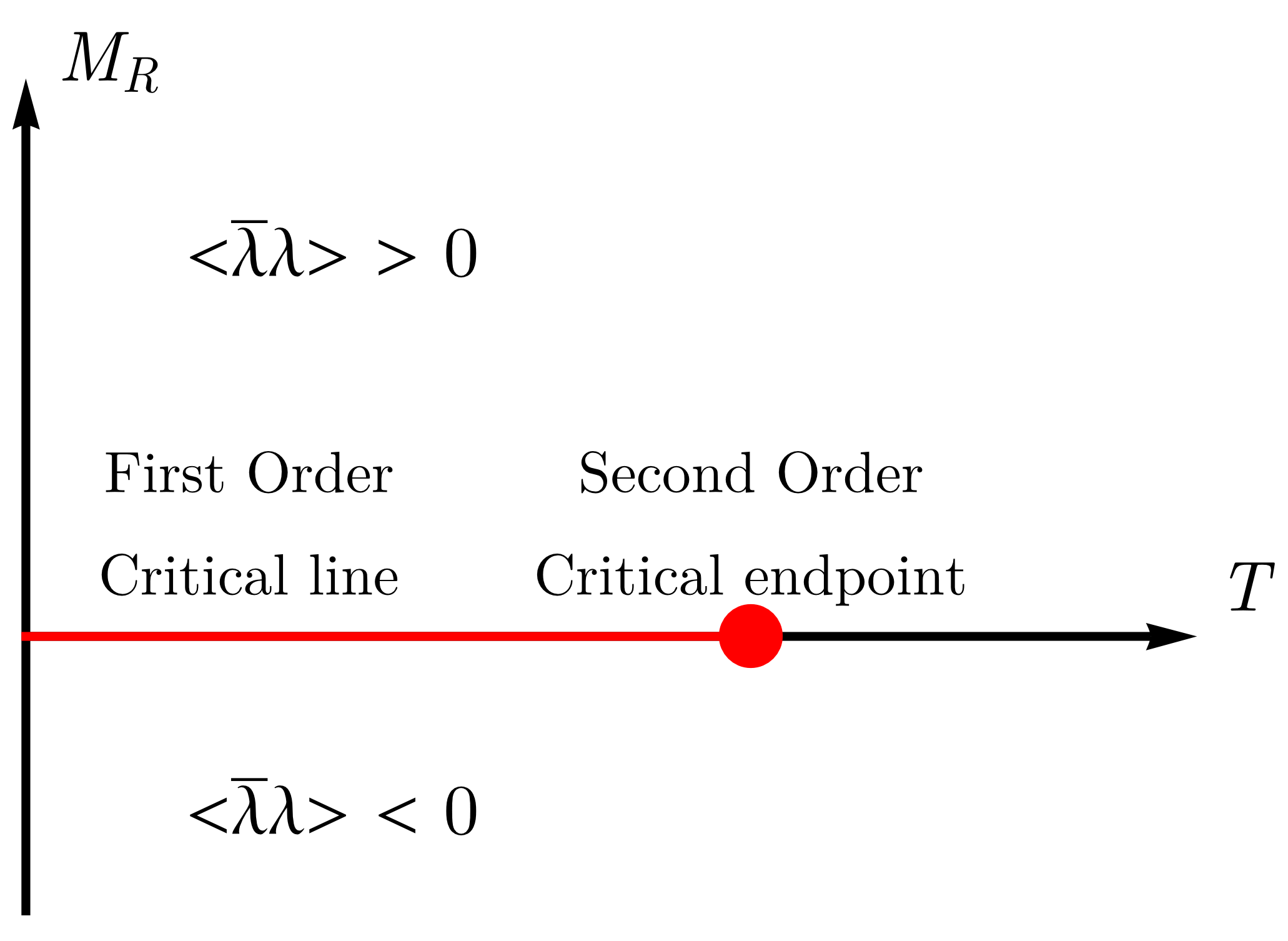
Figure 1: Expected phase diagram for chiral symmetry breaking of $\mathcal{N}=1$ SYM with gauge group SU(2). The chiral condensate $\langle\bar{\lambda}\lambda\rangle$ is the order parameter of the chiral phase transition. Each non-zero value of the renormalised gluino mass $M_{R}$ introduces a source of chiral symmetry breaking. At low temperatures, moving from positive to negative gluino mass $M_{R}$, the chiral condensate jumps from a positive to a negative expectation value. The phase transition is therefore of first order with a coexistence of two phases. The line of first order phase transitions is expected to terminate in a second order endpoint.

The $\mathcal{N}=1$ SYM has a classical U(1)_A axial symmetry, meaning that the transformation

$$\lambda\rightarrow\lambda^{\prime}=\exp{(-\mathrm{i}\hskip 1.0pt\omega\gamma_{5})}\lambda$$ (16)

leaves the action invariant when the gluino mass is exactly zero. This symmetry is known as the R-symmetry U(1)_R and it corresponds to the relative rotation of the left- and the right-handed Weyl components of the gluino field $\lambda$.

Beyond the classical level, quantum fluctuations break chiral symmetry by a term proportional to the gauge coupling and to the number of colours:

$$\partial_{\mu}J^{\mu}_{5}=\partial_{\mu}(\bar{\lambda}\gamma^{\mu}\gamma_{5}\lambda)=N_{c}\frac{g^{2}}{32\pi^{2}}\epsilon_{\mu\nu\rho\sigma}F^{\mu\nu}F^{\rho\sigma}.$$ (17)

The dependence on $N_{c}$ is absent in QCD, and it is typical of gauge models with fermions in the adjoint representation.

The anomalous contribution to the axial transformations can be absorbed in the periodicity of the parameter $\Theta$:

$$\Theta\rightarrow\Theta-2N_{c}\,\omega,$$ (18)

if the angle $\omega$ assumes one of the values $\omega=\frac{n\pi}{N_{c}}$, $n=0,\ldots,2N_{c}-1$. The remaining chiral symmetries thus from the group $Z_{2N_{c}}$. Numerical investigations [29] have confirmed the conjecture [27, 30, 31] that this invariance is spontaneously broken at zero temperature by a non-vanishing expectation value of the gluino condensate $\langle\bar{\lambda}\lambda\rangle\neq 0$ to a remaining $Z_{2}$ symmetry corresponding to the sign flip $\lambda\rightarrow-\lambda$. The complete pattern of chiral symmetry breaking is thus

$$\mathrm{U}(1)_{A}\rightarrow Z_{2N_{c}}\rightarrow Z_{2}.$$ (19)

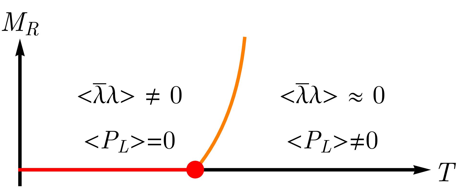
(a) Coincident phase transitions

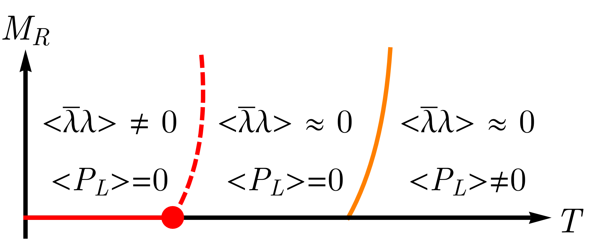
(b) Mixed phases allowed

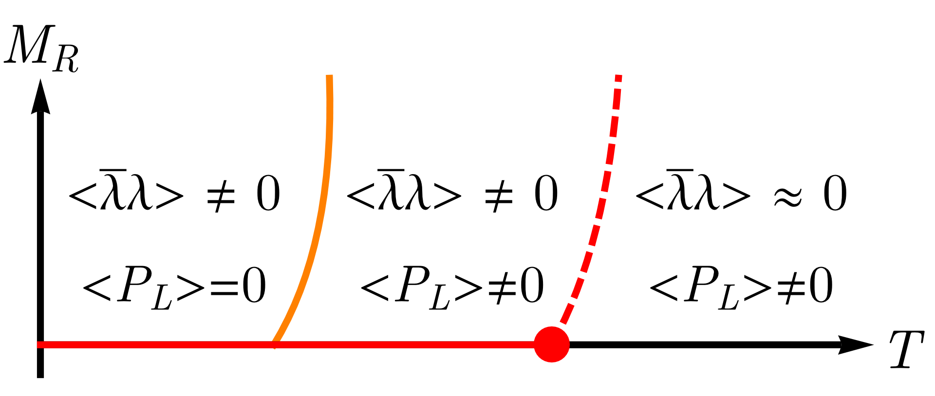
(c) Mixed phases allowed

Figure 2: Possible scenarios for the phase diagram of $\mathcal{N}=1$ SYM. The two chiral phases are separated by a crossover for $M_{R}\neq 0$ (dashed red lines) and by a phase transition in the massless limit. The orange line represents the deconfinement phase transition, present for any value of $M_{R}$. (a) In the supersymmetric limit chiral and deconfinement transition coincide. (b) A mixed confined phase occurs with chiral symmetry restored. (c) A mixed deconfined phase occurs with chiral symmetry broken.

The phase transition associated with the spontaneous breaking $Z_{2N_{c}}\rightarrow Z_{2}$ is of first order at zero temperature, related to the jump of the expectation value of the chiral condensate. The system is in this respect similar to a $Z_{N_{c}}$ Ising model ($Z_{N_{c}}=Z_{2N_{c}}/Z_{2}$), with the gluino condensate corresponding to the spontaneous magnetisation and the renormalised gluino mass to the external magnetic field. This similarity suggests that for the gauge group SU(2) there is a critical temperature $T_{c}^{\textrm{chiral}}$ of a second order phase transition and a phase with restored $Z_{4}$ symmetry at high temperatures, see Fig. 1.

There are three possible scenarios for the relation of deconfinement and chiral symmetry restoration. $T_{c}^{\textrm{chiral}}$ might coincide with the deconfinement transition temperature $T_{c}^{\textrm{deconf.}}$, but there is no restriction to this scenario from first principles. If they do not coincide either a mixed deconfined phase with broken chiral symmetry or a mixed confined phase with restored chiral symmetry exists, see Fig. 2.

In addition, the remaining part of the U(1)_R symmetry broken by the anomaly could be effectively restored in high temperature limit.

5 Simulation algorithms

In order to perform Monte Carlo simulations of $\mathcal{N}=1$ SYM, the gluino field is integrated out in the path integral. For Majorana fermions the result is the Pfaffian of the Wilson-Dirac operator

$$Z=\int DU\ \mathrm{Pf}(CD_{W})\exp{(-S_{g})}.$$ (20)

The Pfaffian of an antisymmetric matrix is related to the square root of the determinant by

$$\mathrm{Pf}(CD_{W})=\mathrm{sign}(\mathrm{Pf}(CD_{W}))\sqrt{\mathrm{det}(D_{W})}.$$ (21)

The additional factor leads to the notorious sign problem of this theory. At a fixed lattice spacing, configurations with a negative Pfaffian sign can appear. This happens in particular at small residual gluino masses close to the supersymmetric limit. These contributions are reduced moving to smaller lattice spacings and the Pfaffian is strictly positive in the continuum limit. It is hence possible to stay in the region where the sign problem is irrelevant. On the other hand, a reliable extrapolation to the supersymmetric limit requires small gluino masses, and negative Pfaffian signs cannot be excluded. We have monitored the Pfaffian signs for the runs with the most critical parameters using the method introduced in [32] to keep this effect under control.

Our simulations have been performed using the Hybrid Monte Carlo algorithm (HMC). We have applied two different approaches for the approximation of the square root of the determinant: an exploratory study was done with a code based on the polynomial (PHMC) approximation; the second, and main part of the work, was performed instead using a new code, based on the rational (RHMC) approximation. The PHMC algorithm is used with one-level stout links in the Wilson-Dirac operator, while the RHMC is used with unsmeared links.

When the renormalised gluino mass is sent to zero, the Wilson-Dirac operator becomes ill-conditioned and the computational demand for the numerical integration of the classical trajectory in the HMC increases drastically. The most reliable approach is therefore to perform the simulations for several non-zero values of the gluino mass and obtain the supersymmetric limit by extrapolation of the results.

6 Scale setting in supersymmetric Yang-Mills theory

The phase diagram of $\mathcal{N}=1$ SYM theory is investigated on lattices of finite size $N_{s}^{3}\times N_{\tau}$ for different values of the bare couplings $\kappa$ and $\beta$. The boundary conditions are anti-periodic in the Euclidean time direction for fermions and periodic in all other cases. In order to convert the bare parameters into physical units the size of the lattice spacing in physical units is needed. This is done by means of the Sommer parameter $r_{0}$ [33] and the $w_{0}$ parameter [34]. The calculation of the scale is based on results of simulations at zero temperature.

At fixed $\beta$ and $\kappa$ the temperature is proportional to the inverse of the number of lattice sites in the temporal direction $N_{\tau}$,

$$T=\frac{1}{N_{\tau}a}.$$ (22)

The continuum limit is obtained when $a\rightarrow 0$ at fixed $T$. The phase transitions are determined as a function of the renormalised value of the residual gluino mass $M_{R}$ that breaks supersymmetry softly. The extrapolation of the transition temperatures to the supersymmetric limit $M_{R}\rightarrow 0$ is the final result of our calculation. It has been shown in a partially quenched setup that $M_{R}$ is proportional to the square of the adjoint pion mass $m_{\text{a--}\pi}$ [26]. For several critical couplings $\beta_{c}^{\textrm{dec}}$ and $\kappa_{c}^{\textrm{dec}}$ of the deconfinement transition the adjoint pion mass is measured in zero temperature simulations on lattices of size $N_{s}^{3}\times 2N_{s}$. These results are summarised in Table A.4. At small values of $m_{\text{a--}\pi}$ the dependence of $M_{R}$ on $1/\kappa$ for fixed $\beta$ is approximately linear. In cases, where zero temperature results at $\beta_{c}^{\textrm{dec}}$ and different values of $\kappa$ were present from previous investigations we apply a linear fit to interpolate $M_{R}$ at $\kappa_{c}^{\textrm{dec}}$.

In the continuum the scaling function is given by the Novikov-Shifman-Vainshtein-Zakharov beta-function [35] to all orders in perturbation theory. From this beta-function the one-loop perturbative scaling of the lattice spacing as a function of the coupling $\beta$ in the supersymmetric limit is given by

$$a(\beta)=\frac{1}{\Lambda}\exp{\left(-\frac{\pi^{2}}{3}\beta\right)}.$$ (23)

However, at finite lattice spacings it is more feasible to consider a non-perturbative scale setting based on measurable scale parameters.

We consider two different observables for the scale setting. The first one is the Sommer parameter $r_{0}/a$ obtained from the static quark-antiquark potential [33]. Since in SYM there is no string breaking for static quarks in the fundamental representation, this scale can be measured in the same way as for pure Yang-Mills theory. The second observable is the recently proposed alternative $w_{0}/a$ [34]. This observable is obtained from the gradient flow of the gauge action density $E$ with $G^{a}_{\mu\nu}$ represented by clover plaquettes,

$$E=\frac{1}{4}G_{\mu\nu}^{a}G_{\mu\nu}^{a}\;.$$ (24)

The gradient flow is defined as continuous smearing procedure using, in our case, the functional derivative of the Wilson plaquette action. The scale parameter $w_{0}/a$ is defined by the flow time $t$, where

$$\left.t\frac{d}{dt}\left[t^{2}\langle E(t)\rangle\right]\right|_{t=w_{0}^{2}}=0.3\;.$$ (25)

The dependence of the observable on the flow time is shown in Fig. 3(a). As expected, the dependence of $t^{2}E$ on $t$ is approximately linear for large $t$.

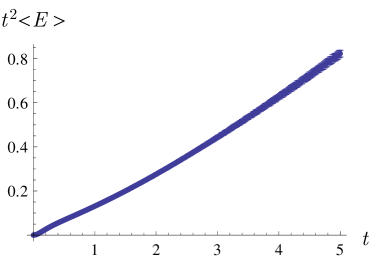
(a) Wilson flow energy

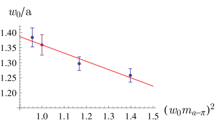
(b) Mass dependence of $w_{0}/a$

Figure 3: a) Expectation value of the gauge energy as a function of the Wilson flow time $t$ on a $14^{4}$ lattice at $\beta=1.65$ and $\kappa=0.1875$. b) Dependence of $w_{0}/a$ on the gluino mass for $\beta=1.62$, see Table A.4. In a mass independent renormalisation scheme, the scale is fixed at a reference gluino mass (in our case $(w_{0}m_{\text{a--}\pi})^{2}=1$, purple point), extracted from a linear fit of the available data.

An advantage of $r_{0}/a$ and $w_{0}/a$ is their weak dependence on the residual gluino mass. In both cases a mild, but not negligible, linear dependence is observed, see Fig. 3(b). As a consequence two different approaches can be applied to set the scale: in a mass dependent renormalisation scheme the scale is set separately at each value of $M_{R}$ and consequently the lattice spacing depends on the gluino mass,

$$a\equiv a(\beta,M_{R}).$$ (26)

In the second approach the lattice spacing is taken to be independent of the gluino mass $M_{R}$,

$$a\equiv a(\beta)\;.$$ (27)

Therefore, in this case the linear behaviour of $w_{0}/a$ and $r_{0}/a$ is interpreted as a physical dependence of their value on the fermion mass [36]. This approach is called mass independent renormalisation scheme and it requires an extrapolation of $r_{0}/a$ and $w_{0}/a$ to a fixed reference value of $M_{R}$, as shown in Fig. 3(b).

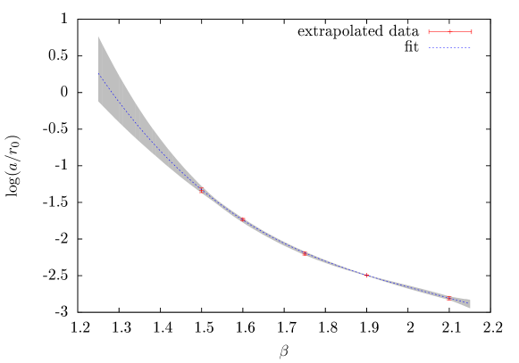
Figure 4: The scale setting of supersymmetric Yang-Mills theory. The figure shows the values of $r_{0}/a$ extrapolated to the chiral limit ($M_{R}=0$).

In our exploratory study, where the PHMC approximation with one-level of stout smearing has been used, the mass independent approach has been applied. From previous investigations we have already some zero temperature results at $\beta=1.6$, $1.75$, $1.9$, and $2.1$, see Table A.2. In these studies the Sommer parameter $r_{0}/a$ has been extrapolated to the value $r_{0}^{e}/a$ at the supersymmetric limit, corresponding to a reference scale of $M_{R}=0$. We have completed the data with additional simulations at $\beta=1.5$, see Table A.1. The dependence of the scale $r_{0}^{e}/a$ on $\beta$ is fitted with a similar parametrisation as used in [37],

$$\log(a/r_{0}^{e})=a_{1}+a_{2}(\beta-2)+a_{3}(\beta-2)^{2}+a_{4}(\beta-2)^{3}\;.$$ (28)

Due to the limited amount of data the error of the coefficients $a_{1}$, $a_{2}$, $a_{3}$, and $a_{4}$ is not reliably obtained from a single fit. To get a better estimate we have assembled several samples of data points by taking values within the given error bounds of each point. With the fits of these samples one obtains a set of curves that determines the error bound of the interpolation, see Fig. 4. This result determines the values of $r_{0}^{e}/a$ for the $\beta$ values without enough data from zero temperature simulations.

In the second part of the work, where the simulations have been performed with the RHMC algorithm and without stout smearing, the scale has been set by the parameter $w_{0}$ and both the mass dependent and independent schemes. In the mass independent scheme $w_{0}$ is extrapolated to the chosen reference point $(w_{0}m_{\text{a--}\pi})^{2}=1$, see Fig. 3(b). This reference point can be accurately extrapolated already from a small number of zero temperature simulations. The obtained value $w_{0}^{e}(\beta)$ is used to fix the scale for all the simulations with the same value of $\beta$. In order to exclude possible systematic errors with this approach we have also applied a mass dependent scale setting prescription, see Table A.4. In that case the scale at $\beta$ and $\kappa$ is set with the value of $w_{0}$ measured at the same combination of the parameters in a zero temperature simulation.

7 The confinement-deconfinement phase transition

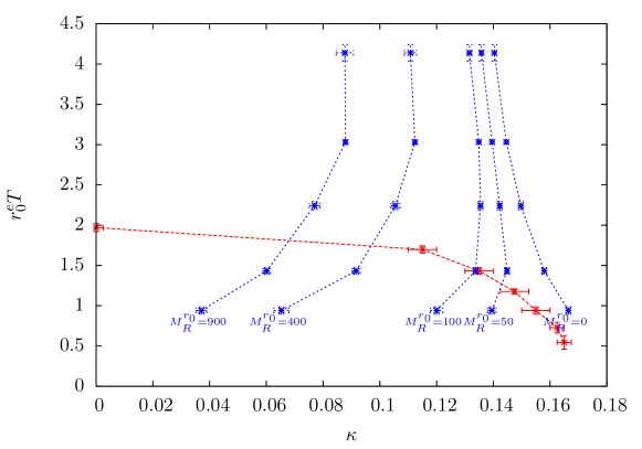
(a) Temperature versus $\kappa$

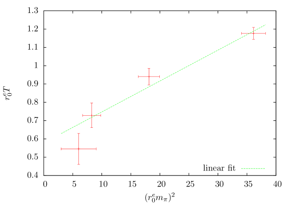
(b) Extrapolation of $T_{c}$

Figure 5: a) The confinement-deconfinement phase transition as a function of the bare parameter $\kappa$ (red line). The simulations are done with one level of stout smearing on $8^{3}\times 4$ and $12^{3}\times 4$ lattices. The blue lines indicate the lines of constant physics, corresponding to a fixed residual mass $M^{r_{0}}_{R}=(r_{0}^{e}m_{\text{a--}\pi})^{2}$. The chiral limit is approached at the line $M_{R}=0$. In these data the scale $r_{0}^{e}$ is fixed to the extrapolated value in the chiral limit. b) Linear extrapolation of the critical temperature to the chiral limit.

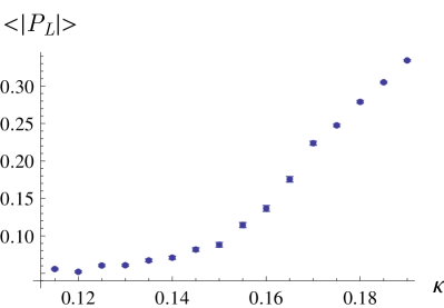
(a) Polyakov loop $\langle P_{L}\rangle$

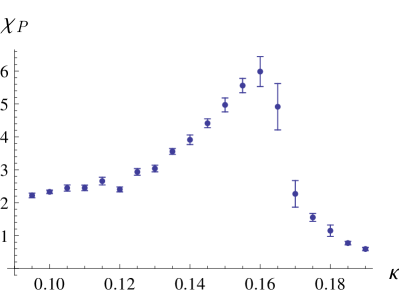
(b) Polyakov loop susceptibility $\chi_{P}$

Figure 6: The expectation value of the Polyakov loop and of its susceptibility on a $12^{3}\times 4$ lattice at $\beta=1.65$.

We have done the first scan of the phase diagram of supersymmetric Yang-Mills theory with the same parameters and settings as in our zero temperature studies of the particle spectrum [21]. One level of stout smearing has been applied in these simulations. They have been performed at fixed lattice size of $N_{s}=8$ and $N_{\tau}=4$. A few runs, to check the finite volume effects, have been done using $N_{s}=12$. We have collected for each value of $\beta$ the critical value $\kappa_{c}^{\textrm{dec}}$ determined by the peak in the Polyakov loop susceptibility. The results can be found in Table A.3 and are represented by the red symbols in Fig. 5(a). The value of $r_{0}^{e}T=(r_{0}^{e}/a)/N_{\tau}$ is calculated with the value of $r_{0}^{e}/a$, for each value of $\beta$, obtained from an interpolation based on Eq. (28).

The red line indicates the transition between confined and deconfined phase for a residual gluino mass $M_{R}$ different from zero. In the limit of $\kappa=0$, i. e. infinite $M_{R}$, the result of pure SU(2) Yang-Mills theory is obtained. Lowering the mass, i.e. increasing $\kappa$, towards the chiral limit the phase transition temperature decreases. Since $N_{\tau}$ is fixed these lower temperatures correspond to a smaller value of $\beta$ and a larger lattice spacing.

The blue symbols in Fig. 5(a) indicate the lines of constant $M^{r_{0}}_{R}\doteq(r_{0}^{e}m_{\text{a--}\pi})^{2}$ in zero temperature simulations. They are based on the results of simulations at $\beta=1.5$, $1.6$, $1.75$, $1.9$, and $2.1$, where theses five values correspond to the five points along each blue line. A linear interpolation of $m_{\text{a--}\pi}$ as a function of $1/\kappa$ has been used. Each of the intersections between the (blue) lines of constant $M_{R}$ and the phase transition (red) line corresponds to the phase transition at temperature $r_{0}^{e}T_{c}$ of a theory with softly broken supersymmetry.

The phase transition of the supersymmetric Yang-Mills theory would correspond to the intersection between the red line and the $M_{R}=0$ line. From these results it can only be estimated to be around $0.5\lesssim r_{0}^{e}T_{c}\lesssim 1.0$. A systematic extrapolation can be done as a function of the physical parameter $M_{R}$ instead of the bare parameter $\kappa$. We take the four largest values of $\kappa$, corresponding to $\beta=1.55,1.50,1.45,1.40$. They are converted to $M_{R}^{r_{0}}$ using the values of $am_{\text{a--}\pi}$ of Table A.1. We can perform a linear fit to determine the critical temperature, see Fig. 5(b). Already with these rough data the phase transition point can thus be estimated to be around

$$r_{0}^{e}T_{c}=0.577(81)\;.$$ (29)

In these first investigations it turned out that much larger statistics and a more precise scale estimation is necessary. Compared to these uncertainties the improvement by stout smearing of the links is not important. We have therefore developed a new more flexible update program and performed a careful investigation in the region with small $M_{R}$ at the phase transition. In that way we have obtained a more reliable extrapolation of the supersymmetric limit without stout smearing.

As explained above, the parameter $w_{0}$ is used as a more recent alternative scale setting. Different spatial and temporal lattice extents are considered with lattice sizes $N_{s}^{3}\times N_{\tau}$ = $8^{3}\times 4$, $12^{3}\times 4$, ${16^{3}\times 4}$, and $10^{3}\times 5$ to estimate the influence of finite size effects and lattice artifacts. For each lattice size, simulations are done with different bare gauge couplings $\beta$ and gluino masses ($\kappa$). The details of the simulations, done at the critical value $\kappa_{c}^{\textrm{dec}}$, are summarised in Table A.5. The autocorrelations between consecutive configurations generated by the HMC algorithm increase drastically near the critical point of the deconfinement transition. We have increased the statistics near the phase transition in order to compensate this effect, and we have investigated accurately the finite volume effects and the scaling behaviour. Hence these points require a huge amount of computer time.

The bare gluino mass ($\kappa$) is varied for each $N_{\tau}$ and for each $\beta$ to locate the point of the deconfinement phase transition $\kappa_{c}^{\textrm{dec}}$. Fig. 6(a) demonstrates this approach for a lattice size $12^{3}\times 4$ and $\beta=1.65$, where the Polyakov loop starts to rise at $\kappa_{c}^{\textrm{dec}}\simeq 0.15$. The point of the phase transition can be determined more clearly by the maximum of the Polyakov loop susceptibility

$$\chi_{P}=V(\langle|P_{L}|^{2}\rangle-\langle|P_{L}|\rangle^{2}).$$ (30)

Here the susceptibility is defined in terms of the modulus of the Polyakov loop. While this choice does not alter the position of the peak, it introduces a non-zero value of $\chi_{P}$ below the critical point.

As can be seen in Fig. 6(b), the location of the transition is found at $\kappa_{c}^{\textrm{dec}}=0.160(5)$, where the susceptibility shows a clear peak. We have found that $\kappa_{c}^{\textrm{dec}}$ defined in this way has only a mild finite volume dependence, which is impossible to distinguish with our current precision.

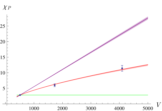
Figure 7: Finite size scaling for the susceptibility $\chi(|P_{L}|)$ at $\beta=1.65$ and $\kappa=0.160$. The red line is the expected scaling for a second order phase transition in the universality class of the $Z_{2}$ Ising model, the purple and the green lines represent instead a first order phase transition and a cross-over, respectively. The coloured shadows indicate the errors from the extrapolation of Eq. (31).

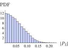
(a) $\kappa=0.100$

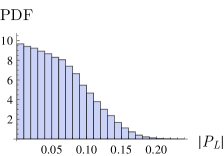
(b) $\kappa=0.125$

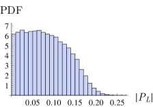
(c) $\kappa=0.145$

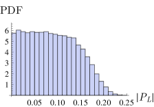
(d) $\kappa=0.150$

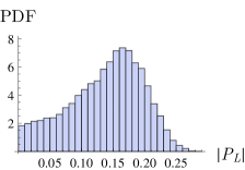
(e) $\kappa=0.160$

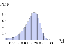
(f) $\kappa=0.165$

Figure 8: Polyakov loop distribution on a $12^{3}\times 4$ lattice at $\beta=1.65$ and various $\kappa$.

The finite size scaling of the susceptibility $\chi_{P}$ contains information about the nature of the phase transition in the infinite volume limit. The susceptibility has a scaling dependence on the volume,

$$\frac{\chi_{P}(V_{1})}{\chi_{P}(V_{2})}=\left(\frac{V_{1}}{V_{2}}\right)^{x},$$ (31)

which is linear for a first order phase transition ($x=1$), flat for a crossover behaviour ($x=0$), and non-linear, with $x=0.657(4)$, for a second order phase transition in the universality class of three-dimensional $Z_{2}$ Ising model [38]. We have obtained the ratios of the Polyakov loop susceptibility for $V_{2}=8^{3}$ and $V_{1}=12^{3},16^{3}$ with $N_{\tau}=4$. The resulting volume dependence is shown in Fig. 7. The Svetitsky-Yaffe conjecture is in good agreement with the data and a possible change from the second order phase transition of pure gauge theory to first order induced by gluinos seems to be excluded.

As a further evidence for this statement the distributions of the Polyakov loop at different values of $\kappa$ demonstrate the slow continuous emergence of a new peak in addition to the central distribution of the absolute value, see Fig. 8. This is in accordance with the divergence of the correlation length at a second order phase transition.

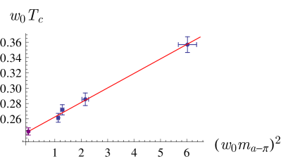
(a) Mass independent

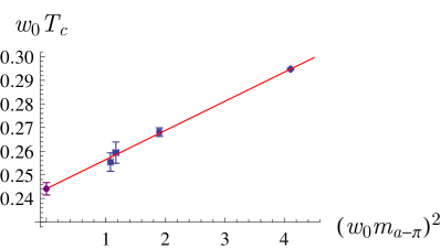
(b) Mass dependent

Figure 9: The critical temperature of the deconfinement phase transition is extrapolated to the supersymmetric limit by extrapolating the results to the point where $(w_{0}m_{\text{a--}\pi})^{2}$ is equal to zero. The four points plotted in the two figures can be found in Table A.4.

The peak of the Polyakov loop susceptibility, Eq. (30), defines a critical combination of bare parameters $(\kappa_{c}^{\textrm{dec}},\beta_{c}^{\textrm{dec}})$, see Table A.5. At these values new simulations have been performed at zero temperature, see Table A.4, to determine the value of the adjoint pion mass in lattice units $am_{\text{a--}\pi}$ and to set the scale. Note that in Table A.4, for each $\beta_{c}^{\textrm{dec}}$, in addition to the result obtained at the corresponding $\kappa_{c}^{\textrm{dec}}$, other values determined at different $\kappa$ are present: these are necessary to extrapolate the mass independent scale $w_{0}^{e}/a$ as explained in Sec. 6. With the previous determinations, the critical temperature and the adjoint pion mass are obtained in dimensionless units, i. e. $w_{0}^{e}T_{c}$ and $w_{0}^{e}m_{\text{a--}\pi}$.

In the mass independent scheme the points $((w_{0}^{e}m_{\text{a--}\pi})^{2},w_{0}^{e}T_{c})$ are linearly interpolated, and the deconfinement temperature is extrapolated to

$$M^{w^{e}_{0}}_{R}\doteq(w_{0}^{e}m_{\text{a--}\pi})^{2}=0.$$ (32)

The linear fit shown in Fig. 9(a) clearly indicates that the deconfinement transition occurs at lower temperatures when the gluino mass is decreased,

$$w_{0}^{e}\,T_{c}(M^{w_{0}^{e}}_{R})=0.0190(22)M^{w^{e}_{0}}_{R}+0.2432(45).$$ (33)

The final extrapolation to the supersymmetric limit $M^{w_{0}^{e}}_{R}=0$ leads to

$$w_{0}^{e}\,T_{c}=0.2432(45),$$ (34)

where the quoted error is only statistical.

As an alternative we employ a mass-dependent renormalisation scheme. The points $((w_{0}m_{\text{a--}\pi})^{2},w_{0}T_{c})$ with $w_{0}$ determined at the same value of the bare parameters $\kappa$ and $\beta$ at the phase transition are linearly interpolated,

$$w_{0}\,T_{c}(M^{w_{0}}_{R})=0.01234(7)M^{w_{0}}_{R}+0.2441(26),$$ (35)

where $M^{w_{0}}_{R}\doteq(w_{0}m_{\text{a--}\pi})^{2}$. The interpolation is shown in Fig. 9(b). The slope is different due to the change of renormalisation scheme. However, the final extrapolation to the supersymmetric limit leads to the compatible result

$$w_{0}T_{c}=0.2441(26),$$ (36)

but with a smaller error due to the more precise determination of the scale for points with heavier gluino masses.

For a comparison of $\mathcal{N}=1$ SYM and pure gauge theory, we computed the scale $w_{0}/a$ at infinite gluino mass on a lattice $18^{4}$ and $\beta=1.829$. The chosen $\beta$ is the critical value for the deconfinement transition of pure SU(2) Yang-Mills theory with a Symanzik improved gauge action at $N_{\tau}=6$ [39]. The measured value of

$$w_{0}/a=1.7649(78)$$ (37)

leads to

$$w_{0}T_{c}=0.2941(13)$$ (38)

for pure SU(2) Yang-Mills theory.

The ratio of the deconfinement temperatures for pure and supersymmetric Yang-Mills theory is thus

$$\frac{T_{c}(\textrm{SYM})}{T_{c}(\textrm{pure Yang-Mills})}=0.826(18).$$ (39)

Introducing physical units by setting $T_{c}=240$ MeV for the critical temperature in pure gauge theory, we obtain a physical value of the deconfinement phase transition temperature for $\mathcal{N}=1$ SU(2) supersymmetric Yang-Mills theory,

$$T_{c}=198(4)\ \textrm{MeV}.$$ (40)

This value is consistent with the one level stout data, see Eq. (29), where we obtain the rough estimate

$$T_{c}=227(32)\ \textrm{MeV}$$ (41)

from our data, assuming $r_{0}^{e}=0.5\ \textrm{fm}$ as in QCD.

In the analysis of the deconfinement transition we have found no evidence for contributions from negative Pfaffians even at the largest values of $\kappa$.

8 The chiral phase transition

The order parameter of the chiral phase transition is the gluino condensate. A non-zero expectation value of this parameter signals the breaking of the $Z_{2}$ remnant of the U(1)_R symmetry. The bare gluino condensate is defined as the derivative of the logarithm of the partition function with respect to the bare gluino mass parameter,

$$\langle\bar{\lambda}\lambda\rangle_{B}\doteq-\frac{T}{V}\frac{\partial}{\partial m}\log(Z(\beta,m)).$$ (42)

Chiral symmetry is broken by our lattice action with the Wilson-Dirac operator for the fermions, and the bare gluino condensate $\langle\bar{\lambda}\lambda\rangle_{B}$ acquires an additive and multiplicative renormalisation:

$$\langle\bar{\lambda}\lambda\rangle_{R}=Z_{\bar{\lambda}\lambda}(\beta)(\langle\bar{\lambda}\lambda\rangle_{B}-b_{0}).$$ (43)

At zero temperature a first order transition is expected when the bare gluino mass is changed, crossing a critical value corresponding to $M_{R}=0$. Close to such a transition the histogram of $\langle\bar{\lambda}\lambda\rangle$ shows a two peak structure in a finite volume. The transition can be identified with the point where the symmetry of the two peaks changes, as done in [29]. Such an analysis is independent of the renormalisation described in Eq. (43). At finite temperatures the first order chiral phase transition extends to a phase transition line at $M_{R}=0$, terminating in a second order end-point. Beyond that point the transition changes from first order to a cross over, see Fig. 2. For this reason, considerations on the renormalisation procedure become important for the precise localisation of the phase transition.

The additive renormalisation is removed by a subtraction of the zero temperature result:

$$\langle\bar{\lambda}\lambda\rangle_{S}=\langle\bar{\lambda}\lambda\rangle_{B}^{T=0}-\langle\bar{\lambda}\lambda\rangle_{B}^{T}\;.$$ (44)

The calculation of the renormalisation constant $Z_{\bar{\lambda}\lambda}(\beta)$ can be avoided in a fixed scale approach, where the bare coupling $\beta$ and $\kappa$ are fixed and the temperature is changed by a variation of $N_{\tau}$.

The bare gluino condensate is obtained from the trace of the inverse Wilson-Dirac operator,

$$-\frac{T}{V}\frac{\partial}{\partial m}\log(Z(\beta,m)) = -\frac{1}{Z(\beta,m)}\frac{T}{V}\frac{\partial}{\partial m}\left\langle\exp{\left(\frac{1}{2}\mathrm{tr}\log(D_{W}(m))\right)}\right\rangle_{S_{g}}$$ (45)

$$= -\frac{T}{V}\left\langle\frac{1}{2}\mathrm{tr}(D_{W}^{-1})\right\rangle.$$

Here and in the following $\langle O\rangle_{S_{g}}$ denotes the functional integral with respect to the gauge part of the action, i. e. $Z(\beta,m)=\left\langle\exp{\left(\frac{1}{2}\mathrm{tr}\log(D_{W}(m))\right)}\right\rangle_{S_{g}}$, where a positive Pfaffian is assumed. The trace of the inverse Wilson-Dirac operator is evaluated with 20 random noise vectors using the stochastic estimator technique.

The simulations are done on a lattice $12^{3}\times N_{\tau}$, with $N_{\tau}\in\{4,\dots,11\}$, $\beta=1.7$, and $\kappa=0.192$. A simulation at zero temperature, i. e. $N_{\tau}=12$, has been performed to determine the adjoint pion mass $am_{\text{a--}\pi}=0.388(9)$ and the value of the scale $w_{0}/a=2.070(38)$.

The subtracted chiral condensate starts to rise at $N_{\tau}\simeq 7$, but its behaviour is quite smooth due the crossover nature of the transition away from the supersymmetric limit, see Fig. 10(a). For a better identification of the pseudo-critical transition point, we determine the peak of the chiral susceptibility $\chi_{c}$. This observable is proportional to the derivative of the gluino condensate and it has connected and disconnected contributions:

$$\chi_{c} = -\frac{T}{V}\frac{\partial^{2}}{\partial m^{2}}\log(Z(g,m))=-\frac{T}{V}\frac{\partial}{\partial m}\left\langle\frac{1}{2}\mathrm{tr}(D_{W}^{-1})\exp{\left(\frac{1}{2}\mathrm{tr}\log(D_{W}(m))\right)}\right\rangle_{S_{g}}$$ (46)

$$= -\frac{T}{V}\left\{\left\langle\frac{1}{4}\mathrm{tr}(D_{W}^{-1})^{2}\right\rangle-\left\langle\frac{1}{4}\mathrm{tr}(D_{W}^{-1})\right\rangle^{2}-\left\langle\frac{1}{2}\mathrm{tr}(D_{W}^{-2})\right\rangle\right\}.$$

The connected contribution is expected to vanish in the supersymmetric limit. In the range of parameters that we have considered in this investigation the disconnected contribution is already dominant and the connected contribution can be neglected for a localisation of the peak, see Fig. 11. In that respect the relevant dynamics of the phase transition is already similar to the one at a vanishing residual gluino mass. Even though the connected contribution is negligible, we consider the complete observable in the following. In that way we ensure that absence of additional systematic uncertainties in our extrapolations.

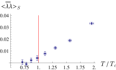
(a) Subtracted chiral condensate

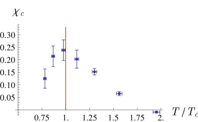
(b) Chiral susceptibility

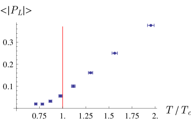
(c) Polyakov loop

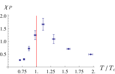
(d) Polyakov loop susceptibility

Figure 10: a-b) Chiral condensate and its susceptibility on a $12^{3}\times N_{\tau}$ lattice at $\beta=1.7$, $\kappa=0.192$; c-d) Polyakov loop and its susceptibility at the same parameters. $T_{c}$ refers to the deconfinement transition temperature obtained from an extrapolation to the supersymmetric limit using Eq. (35).

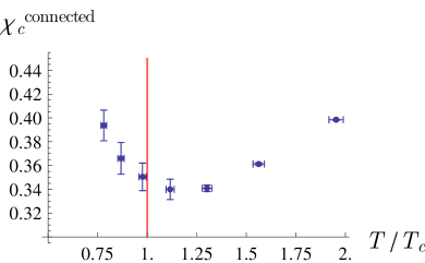
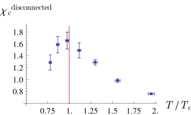
Figure 11: Comparison of connected (left) and disconnected (right) contributions to the chiral susceptibility on a $12^{3}\times N_{\tau}$ lattice at $\beta=1.7$, $\kappa=0.192$.

The results of our simulation are shown in Fig. 10(b). Even though there is quite a broad central region, a visible peak can be identified corresponding to the value at $N_{\tau}=9$. For comparison, the Polyakov loop is shown in Fig. 10(c). It acquires a non-vanishing expectation value at $N_{\tau}=8$. This small deviation is still consistent with the scenario of a chiral symmetry restoration and a deconfinement phase transition at the same temperature.

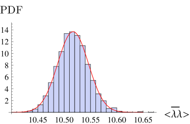
(a) $N_{\tau}=5$

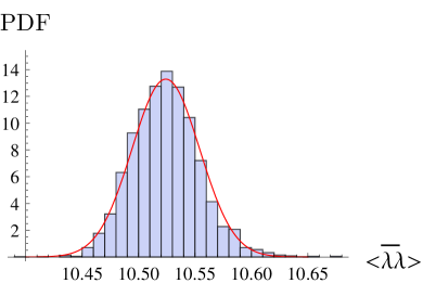
(b) $N_{\tau}=6$

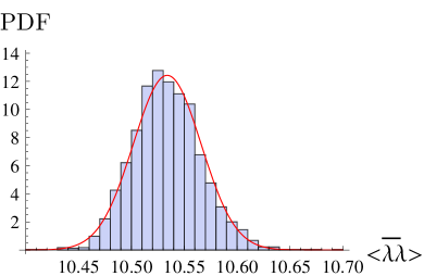
(c) $N_{\tau}=7$

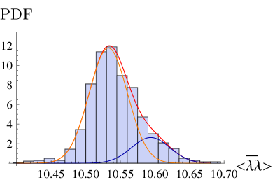
(d) $N_{\tau}=8$

Figure 12: Distributions of the chiral condensate on $12^{3}\times N_{\tau}$ lattices at $\beta=1.7$ and $\kappa=0.194$. For $N_{\tau}=5$ the distribution is compatible with a single Gaussian, while for $N_{\tau}=8$ a second peak emerges.

In order to provide an upper limit for the chiral symmetry restoration temperature, we have done new simulations approximately at the supersymmetric limit, i. e. around the value of $\kappa$ where the adjoint pion mass is expected to vanish, following the approach of [29]. This corresponds to $\kappa=0.194$ at $\beta=1.7$. The lattice sizes were chosen to be $12^{3}\times N_{\tau}$ with $N_{\tau}\in\{5,6,7,8\}$. Note that these simulations cannot be done at large values of $N_{\tau}$, due to the long time needed for a convergence of the conjugate gradient algorithm in that limit. The distributions are displayed in Fig. 12. At high temperatures, like $N_{\tau}=5$, the distribution is close to a Gaussian without any indications for a double peak in the gluino condensate. At $N_{\tau}=8$, on the other hand, we observe a small second peak emerging from the distribution. Therefore, at these low temperatures the transition, close to the supersymmetric limit, becomes consistent with a first order chiral phase transition. Moreover, this suggests that the transition happens in the region between $N_{\tau}=7$ and $N_{\tau}=8$. It is another indication that the chiral phase transition and the deconfinement transition are close to each other: assuming that the value of $w_{0}$ does not change so much going from $\kappa=0.192$ to $\kappa=0.194$ we are able to estimate an upper limit for the supersymmetric chiral critical temperature: $T_{\chi}(M_{R}=0)\lesssim 1.5\,T_{c}$.

We have checked our assumption of a positive Pfaffian by a measurement of its sign on 200 configurations. At $\kappa=0.192$ we have found no contribution, whereas at $\kappa=0.194$ around $8\%$ of the configurations have a negative sign on the $12^{3}\times 8$ lattice. Hence the simulations at the supersymmetric limit provide only an estimate of the transition point. In further studies the contributions with a negative sign have to be taken into account more carefully; alternatively, with a larger amount of computing time, the supersymmetric limit can extrapolated from a region without a relevant sign problem.

9 Conclusions

We have investigated the deconfinement and the chiral phase transitions in $\mathcal{N}=1$ supersymmetric Yang-Mills theory. Different from the case of QCD, the Polyakov loop is a well-defined order parameter at all values of the gluino mass, and the deconfinement transition can be identified in an unambiguous way. The U(1)_R chiral symmetry is only partially broken by the anomaly and a remnant $Z_{2N_{c}}$ symmetry survives. The expectation value of the gluino condensate is the order parameter for the breaking of this remnant symmetry down to $Z_{2}$.

We have investigated the dependence of both order parameters on the temperature and on the gluino mass. We have determined the temperature, where the deconfinement phase transition takes place, with a good accuracy, and extrapolated the transition temperature in the supersymmetric limit. Different scale setting prescriptions lead to consistent results, indicating the reliability of the result. The transition happens at a temperature, which is around 80% of the transition temperature in pure Yang-Mills theory.

The identification of the chiral phase transition point, on the other hand, needs more effort, since the transition becomes a crossover at finite gluino masses. In a fixed scale approach we have identified the transition region taking also the renormalisation into account. We were able to narrow the range for the chiral transition down to a region close to the deconfinement transition. This situation can be compared with $N_{f}=2$ adjoint QCD (aQCD), a theory similar to SYM. In the case of aQCD, there exists a mixed phase with deconfinement but a broken chiral symmetry. The deconfinement temperature is eight times smaller than the point of chiral symmetry restoration [40]. From this perspective, SYM appears to be more similar to QCD, where the deconfinement and chiral symmetry restoration seem to occur at the same temperature.

In order to confirm scenario (a) of Fig. 2 with coincident phase transitions, it will be necessary to perform simulations in more parameter points, with higher statistics, and on larger lattices. A study of the finite size scaling is of great importance to test the existence of a second order endpoint for the chiral phase transition in the supersymmetric limit.

Presently we have been able to study the phase transitions only at rather low values of $\beta$, i. e. at relatively large lattice spacings. At these parameters there is still a considerable deviation from the degeneracy of the particle masses in supermultiplets. Hence studies at larger values of $N_{\tau}$ are needed for reliable extrapolations to the supersymmetric limit. This is the largest source of a systematic uncertainty for our current determination of the deconfinement transition point.

In the future we also plan to study different numbers of colours $N_{c}$, and different boundary conditions, since the phase transitions seem to be sensitive to these parameters.

Appendix A Details of the simulations

$N_{\tau}$	$N_{s}$	$\beta$	$\kappa$	$r_{0}/a$	$am_{\text{a--}\pi}$	$N_{\text{conf.}}$
32	16	1.65	0.1150	–	2.206(14)	600
32	16	1.55	0.1475	–	1.2770(24)	621
32	16	1.5	0.155	–	1.1316(34)	800
32	16	1.5	0.158	2.68(6)	0.97863(84)	2036
32	16	1.5	0.160	2.85(3)	0.8570(20)	2177
32	16	1.5	0.162	3.11(9)	0.7085(19)	2076
32	16	1.5	0.163	3.15(8)	0.6199(12)	2001
32	16	1.5	0.164	3.34(8)	0.5066(26)	1720
24	12	1.45	0.1625	–	0.9865(25)	1000
24	12	1.40	0.145	–	1.722(40)	1199
24	12	1.40	0.150	–	1.563(72)	1599
24	12	1.40	0.153	–	1.501(13)	1800
24	12	1.40	0.155	–	1.434(18)	1999
24	12	1.40	0.160	–	1.2858(13)	1240

Table A.1: Parameters for the additional zero temperature simulations with one level of stout smearing. At $\beta=1.5$ the value of $r_{0}/a$ is extrapolated to the supersymmetric limit.

$\beta$	1.5	1.6	1.75	1.9	2.1
$r_{0}^{e}/a$	3.81(12)	5.93(5)	9.02(18)	12.20(12)	16.56(39)

Table A.2: Values of $r_{0}^{e}/a$ determined for different values of $\beta$. The values for $\beta=1.6$ and $1.75$ can be found in our previous publications; the others are presented here for the first time. The value at $\beta=1.5$ is determined from the extrapolation of the zero temperature results in Table A.1.

$N_{\tau}$	$N_{s}$	$\beta$	$N_{\text{conf.}}$	$\kappa_{c}^{\textrm{dec}}$
4	12	1.60	2500	0.140(15)
4	12	1.50	2500	0.155(10)
4	8	1.70	20000	0.0000(25)
4	8	1.65	20000	0.1150(50)
4	8	1.60	20000	0.1350(50)
4	8	1.55	20000	0.1475(50)
4	8	1.50	20000	0.1550(50)
4	8	1.45	20000	0.1625(25)
4	8	1.40	20000	0.1650(25)

Table A.3: The number of measured configurations $N_{\text{conf.}}$, produced at the $\kappa_{c}^{\textrm{dec}}$ value, used for estimating the deconfinement transition, using one level of stout smearing. The parameters are the same as in our zero temperature investigations of the particle spectrum [21].

$N_{\tau}$	$N_{s}$	$\beta$	$\kappa$	$am_{\text{a--}\pi}$	$w_{0}/a$	$w_{0}^{e}/a$
20	10	1.65	0.1600	1.7182(09)	1.179(02)	1.428(36)
20	10	1.65	0.1825	1.1138(20)	1.310(09)	1.428(36)
20	10	1.65	0.1850	1.0277(24)	1.340(09)	1.428(36)
20	10	1.65	0.1875	0.9342(22)	1.326(13)	1.428(36)
20	10	1.62	0.1900	0.9398(26)	1.258(23)	1.359(34)
20	10	1.62	0.1925	0.8331(29)	1.297(23)	1.359(34)
20	10	1.62	0.1950	0.7067(44)	1.384(31)	1.359(34)
20	10	1.60	0.1950	0.8159(62)	1.277(20)	1.307(30)
20	10	1.60	0.1975	0.6868(40)	1.351(26)	1.307(30)
20	10	1.60	0.2000	0.4980(58)	1.553(31)	1.307(30)

Table A.4: The table summarises the zero temperature measurements done for setting the scale without stout smearing. $w_{0}/a$ is the mass dependent value while $w_{0}^{e}/a$ is the mass independent one, i. e. obtained by extrapolation to $(w_{0}m_{\text{a--}\pi})^{2}=1$.

$N_{\tau}$	$N_{s}$	$\beta$	$N_{\text{conf.}}$	$\tau$	$\kappa_{c}^{\textrm{dec}}$
4	8	1.65	150000	400	0.1600(50)
4	12	1.65	80000	1100	0.1600(50)
4	16	1.65	40000	1600	0.1580(50)
5	15	1.65	20000	1500	0.1850(25)
5	15	1.62	20000	1500	0.1925(20)
5	15	1.60	20000	1500	0.1950(20)

Table A.5: The table summarises the number of measurements $N_{\text{conf.}}$, produced at the $\kappa_{c}^{\textrm{dec}}$ value, for estimating the deconfinement transition using the action without stout smearing. The autocorrelation time $\tau$ is computed for the Polyakov loop at the critical point.

References

- [1] J. Engels, J. Fingberg and M. Weber, Nucl. Phys. B 332 (1990) 737.
- [2] B. Lucini, M. Teper and U. Wenger, Phys. Lett. B 545 (2002) 197, [arXiv: hep-lat/0206029 ].
- [3] Y. Aoki, G. Endrodi, Z. Fodor, S. D. Katz and K. K. Szabo, Nature 443 (2006) 675, [arXiv: hep-lat/0611014 ].
- [4] Y. Aoki, Z. Fodor, S. D. Katz and K. K. Szabo, JHEP 0601 (2006) 089, [arXiv: hep-lat/0510084 ].
- [5] A. Bazavov et al., Phys. Rev. D 80 (2009) 014504, [arXiv: 0903.4379 [hep-lat]].
- [6] Y. Aoki, Z. Fodor, S. D. Katz and K. K. Szabo, Phys. Lett. B 643 (2006) 46, [arXiv: hep-lat/0609068 ].
- [7] S. Borsanyi et al. [Wuppertal-Budapest Collaboration], JHEP 1009 (2010) 073, [arXiv: 1005.3508 [hep-lat]].
- [8] J. M. Maldacena, Adv. Theor. Math. Phys. 2 (1998) 231, [arXiv: hep-th/9711200 ].
- [9] S. S. Gubser and A. Karch, Ann. Rev. Nucl. Part. Sci. 59 (2009) 145, [arXiv: 0901.0935 [hep-th]].
- [10] L. Girardello, M. T. Grisaru and P. Salomonson, Nucl. Phys. B 178 (1981) 331.
- [11] T. E. Clark and S. T. Love, Nucl. Phys. B 217 (1983) 349.
- [12] A. K. Das, Physica A 158 (1989) 1.
- [13] O. Aharony, J. Sonnenschein and S. Yankielowicz, Annals Phys. 322 (2007) 1420, [arXiv: hep-th/0604161 ].
- [14] A. Armoni, M. Shifman and G. Veneziano, in: Shifman, M. (ed.) et al.: From fields to strings, vol. 1, 353-444, [arXiv: hep-th/0403071 ].
- [15] A. Armoni, M. Shifman and G. Veneziano, Phys. Rev. Lett. 91 (2003) 191601, [arXiv: hep-th/0307097 ].
- [16] L. Girardello, M. Petrini, M. Porrati and A. Zaffaroni, Nucl. Phys. B 569 (2000) 451, [arXiv: hep-th/9909047 ].
- [17] I. Montvay, Nucl. Phys. B 466 (1996) 259, [arXiv: hep-lat/9510042 ].
- [18] G. Veneziano and S. Yankielowicz, Phys. Lett. B 113 (1982) 231.
- [19] G. R. Farrar, G. Gabadadze and M. Schwetz, Phys. Rev. D 58 (1998) 015009, [arXiv: hep-th/9711166 ].
- [20] G. Bergner, T. Berheide, I. Montvay, G. Münster, U. D. Özugurel and D. Sandbrink, JHEP 1209 (2012) 108, [arXiv: 1206.2341 [hep-lat]].
- [21] G. Bergner, I. Montvay, G. Münster, U. D. Özugurel and D. Sandbrink, JHEP 1311 (2013) 061, [arXiv: 1304.2168 [hep-lat]].
- [22] G. Bergner, JHEP 1001 (2010) 024, [arXiv: 0909.4791 [hep-lat]].
- [23] M. Kato, M. Sakamoto and H. So, JHEP 0805 (2008) 057, [arXiv: 0803.3121 [hep-lat]].
- [24] G. Curci and G. Veneziano, Nucl. Phys. B 292 (1987) 555.
- [25] H. Suzuki, Nucl. Phys. B 861 (2012) 290, [arXiv: 1202.2598 [hep-lat]].
- [26] G. Münster and H. Stüwe, JHEP (2014), in press, [arXiv: 1402.6616 [hep-th]].
- [27] D. Amati, K. Konishi, Y. Meurice, G. C. Rossi and G. Veneziano, Phys. Rept. 162 (1988) 169.
- [28] B. Svetitsky and L. G. Yaffe, Nucl. Phys. B 210 (1982) 423.
- [29] R. Kirchner, I. Montvay, J. Westphalen, S. Luckmann and K. Spanderen, Phys. Lett. B 446 (1999) 209, [arXiv: hep-lat/9810062 ].
- [30] N. Seiberg, Phys. Rev. D 49 (1994) 6857, [arXiv: hep-th/9402044 ].
- [31] N. Seiberg, Nucl. Phys. B 435 (1995) 129, [arXiv: hep-th/9411149 ].
- [32] G. Bergner and J. Wuilloud, Comput. Phys. Commun. 183 (2012) 299, [arXiv: 1104.1363 [hep-lat]].
- [33] R. Sommer, Nucl. Phys. B 411 (1994) 839, [arXiv: hep-lat/9310022 ].
- [34] S. Borsanyi et al., JHEP 1209 (2012) 010, [arXiv: 1203.4469 [hep-lat]].
- [35] V. A. Novikov, M. A. Shifman, A. I. Vainshtein and V. I. Zakharov, Nucl. Phys. B 229 (1983) 381.
- [36] A. K. De, A. Harindranath and J. Maiti, [arXiv: 0803.1281 [hep-lat]].
- [37] S. Necco and R. Sommer, Nucl. Phys. B 622 (2002) 328, [arXiv: hep-lat/0108008 ].
- [38] A. M. Ferrenberg and D. P. Landau. Phys. Rev. B 44 (1991) 5081.
- [39] G. Cella, G. Curci, R. Tripiccione and A. Vicere, Phys. Rev. D 49 (1994) 511, [arXiv: hep-lat/9306011 ].
- [40] F. Karsch and M. Lütgemeier, Nucl. Phys. B 550 (1999) 449, [arXiv: hep-lat/9812023 ].