D numbers theory: a generalization of Dempster-Shafer evidence theory

Abstract

Efficient modeling of uncertain information in real world is still an open issue. Dempster-Shafer evidence theory is one of the most commonly used methods. However, the Dempster-Shafer evidence theory has the assumption that the hypothesis in the framework of discernment is exclusive of each other. This condition can be violated in real applications, especially in linguistic decision making since the linguistic variables are not exclusive of each others essentially. In this paper, a new theory, called as D numbers theory (DNT), is systematically developed to address this issue. The combination rule of two D numbers is presented. An coefficient is defined to measure the exclusive degree among the hypotheses in the framework of discernment. The combination rule of two D numbers is presented. If the exclusive coefficient is one which means that the hypothesis in the framework of discernment is exclusive of each other totally, the D combination is degenerated as the classical Dempster combination rule. Finally, a linguistic variables transformation of D numbers is presented to make a decision. A numerical example on linguistic evidential decision making is used to illustrate the efficiency of the proposed D numbers theory.

1 Introduction

Quantitative handling incomplete, uncertain and imprecise information data warrants the use of soft computing methods [1]. Soft computing methods such as fuzzy set theory [2], rough set [3, 4], Dempster-Shafer evidence theory [5, 6] can essentially provide rational solutions for complex real-world problems. The traditional Bayesian (subjectivist) probability approach cannot differentiate between aleatory and epistemic uncertainties and is unable to handle non-specific, ambiguous and conflicting information without making strong assumptions. These limitations can be partially addressed by the application of Dempster-Shafer evidence theory, which was found to be flexible enough to combine the rigor of probability theory with the flexibility of rule-based systems [7, 8]. Due to its efficiency to handle uncertain information, evidence theory is widely used in many applications such as pattern recognition[9], evidential reasoning [10, 11], complex network and systems [12, 13], DS/AHP [14, 15, 16, 17, 18, 19, 20, 21, 22, 23] and other decision making fields [24, 25, 26, 27, 28, 29, 30].

However, there are some limitations in the classical Dempster-Shafer evidence theory. One of the well known problems is the conflict management when evidence highly conflicts, which is heavily studied. However, some other issues are paid little attention. For example, the elements in the frame of discernment must be mutually exclusive which has greatly limited its practical application [31, 32]. For example, it is not correct to have a basic probability assignment as $m\{good\}=0.8,m\{good,verygood\}=0.2$, since the linguistic variable $verygood$ is not exclusive of the other linguistic variable $good$.

Recently, some applications of D numbers to represent uncertain information has been reported, which is an extension of Dempster-Shafer evidence theory [31, 32, 33, 34] . D numbers can effectively represent uncertain information since that the exclusive property of the elements in the frame of discernment is not required, and the completeness constraint is released if necessary. Due to the propositions of applications in the real word could not be strictly mutually exclusive, these two improvements are greatly beneficial. To get a more accurate uncertain data fusion, a discounting of D numbers based on the exclusive degree is necessary. However, some key issues on D numbers are not yet well addressed. For example, it is necessary to develop a reasonable combination rule of D numbers. In addition, similar to the pignistic probability transformation in belief function theory, the transformation of D numbers into linguistic variables to make a final decision is inevitable. To address these issues, the D numbers theory (DNT) is systematically developed in this paper.

The rest of the paper is organized as follows. Section 2, some preliminaries are briefly introduced. The D numbers theory is presented in Section 3. The application in linguistic decision making is used to illustrate the efficiency of the proposed DNT. Conclusions are given in Section 5.

2 Preliminaries

2.1 Fuzzy set theory

Fuzzy set theory is widely used in uncertain modelling [35, 36]. In some decision makings, assessments are given by natural language in the qualitative form. These linguistic variables can be assessed by means of linguistic terms [37, 38, 39] which is proposed by Zadeh.

Definition 1

Let $X$ be a universe of discourse. Where $\widetilde{A}$ is a fuzzy subset of $X$; and for all $x\in X$ there is a number ${\mu_{\widetilde{A}}}(x)\in[0,1]$ which is assigned to represent the membership of $x$ in $A$, and is called the membership of $\widetilde{A}$. [2].

Definition 2

A fuzzy set $\widetilde{A}$ of the universe if discourse $X$ is convex if and only if for all $x_{1}$, $x_{2}$ in $X$,

$${\mu_{\widetilde{A}}}(\lambda{x_{1}}+(1-\lambda){x_{2}})\geq\min({\mu_{\widetilde{A}}}({x_{1}}),{\mu_{\widetilde{A}}}({x_{2}}))$$ (1)

where $\lambda\in[0,1]$.

Definition 3

A triangular fuzzy number $\widetilde{A}$ can be defined by a triplet(a, b, c), as shown in Fig. 1.

$${\mu_{\widetilde{A}}}(x)=\left\{{\begin{array}[]{*{20}{c}}{0,}&{x<a}\\ {\frac{{x-a}}{{b-a}},}&{a\leq x\leq b}\\ {\frac{{c-x}}{{c-b}},}&{b\leq x\leq c}\\ {0,}&{x>c}\end{array}}\right.$$ (2)

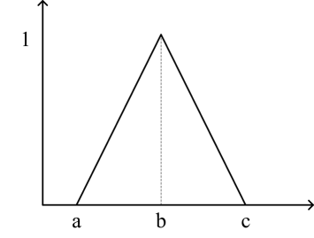
Figure 1: The membership function.

2.1.1 Linguistic variable

The concept of a linguistic variable is very useful in dealing with situations which are too complex or poorly-defined to be reasonably described in conventional quantitative expressions. Linguistic variables are represented in words, sentences or artificial languages, where each linguistic value can modeled by a fuzzy set [40]. In this paper, the importance weights of various criteria and the ratings of qualitative criteria are considered as linguistic variables. These linguistic variables can be expressed in positive triangular fuzzy numbers, as shown in Tables 1 and 2.

Table 1: Linguistic variables for the importance weight of each criterion

Very low (VL)	(0,0,0.1)
Low (L)	(0,0.1,0.3)
Medium low (ML)	(0.1,0.3,0.5)
Medium (M)	(0.3,0.5,0.7)
Medium high (MH)	(0.5,0.7,0.9)
High (H)	(0.7,0.9,1.0)
Very High (VH)	(0.9,1.0,1.0)

Table 2: Linguistic variables for the importance weight of each criterion

Very poor (VP)	(0,0,1)
Poor (P)	(0,1,3)
Medium poor (MP)	(1,3,5)
Fair (F)	(3,5,7)
Medium goog (MG)	(5,7,9)
Good (G)	(7,9,10)
Very good (VG)	(9,10,10)

2.2 Dempster-Shafer (DS) theory of evidence

Let $\Theta$ denote a finite nonempty set of mutually exclusice and exhaustive hypotheses, called the frame of decernment.

Definition 4

A mass function is a mapping m: $2^{\Theta}\to[0,1]$, which satisfies:

$$m(\emptyset)=0\quad and\quad\sum\limits_{A\subseteq\Theta}{m(A)=1}.$$ (3)

A mass function is also called a basic probability assignment(BPA) to all subsets of $\Theta$.

Definition 5

The belief Bel(A) and plausibility Pl(A) measures of an event A $\subseteq$ $\Theta$ can be defined as

$$Bel(A)=\sum\limits_{A_{i}:A_{i}\subseteq A}{m(A_{i})},Pl(A)=\sum\limits_{A_{i}:A_{i}\cap A\neq\emptyset}{m(A_{i})}.$$ (4)

The belief Bel(A) and Plausibility Pl(A) measures can be regarded as lower and upper bounds for the probability of A according to [41, 42]. Let $p_{i}$ be some unknown probability of the i-th element of the $\Theta$, then the probability distribution p = $(p_{1},p_{2},$…,$p_{m})$ satisfies the following inequalities for all focal elements A:

Bel(A) $\leq$ $\sum\limits_{i:u_{i}\in A}{p_{i}}$ $\leq$ Pl(A).

Definition 6

Discounting Evidences: If a source of evidence provides a mass function $m$ which has probability $\alpha$ of reliability. Then the discounted belief m^′ on $\Theta$ is defined as:

$$m^{\prime}(A)=\alpha m(A),\quad\forall A\subset\Theta,A\neq\Theta.$$ (5)

$$m^{\prime}(\Theta)=1-\alpha+\alpha m(\Theta).$$ (6)

All mass function is discounted by $\alpha$, which is called discount coefficient.

Definition 7

Dempster’s rule of combination, denoted by ${(m_{1}\oplus m_{2})}($also called the orthogonal sum of $m_{1}$ and $m_{2})$, is defined as follows:

$$m(A)=\frac{1}{{1-k}}\sum\limits_{B\cap C=A}{m_{1}(B)m_{2}(C)}.$$ (7)

where

$$k=\sum\limits_{B\cap C=\emptyset}{m_{1}(B)m_{2}(C)}.$$ (8)

Note that $k$ is called the normalization constant of the orthogonal sum ${(m_{1}\oplus m_{2})}$. The coefficient $k$ is also called as the conflict coefficient between $m_{1}$ and $m_{2}$, denoted as $\mathop{m}\nolimits_{\oplus}(\emptyset)$ in the following of the paper.

2.3 Pignistic probability transformation(PPT) [43]

Definition 8

Beliefs manifest themselves at two levels - the credal level(from credibility) where belief is entertained, and the pignistic level where beliefs are used to make decisions. The term ”pignistic” was proposed by Smets [43] and originates from the word pignus, meaning ’bet’ in Latin. Pignistic probability is used for decision-making and uses Principle of Insufficient Reason to derive from BPA. It has been increasingly used in recent years [44, 45, 46]. It represents a point estimate in a belief interval and can be determined as:

$$BetP(B)=\sum\limits_{A\in\Theta}{m(A)}\frac{{\left|{B\cap A}\right|}}{{\left|A\right|}}.$$ (9)

where $\left|A\right|$ denotes the number of elements of $\Theta$ in $A$.

3 D numbers theory

In this section, the D numbers theory is developed systematically. There are three main parts of this theory, namely the uncertainty modelling, the combination of D numbers and the decision making based on linguistic variable transformation. These parts are detailed as follows.

3.1 Definition of D numbers

In the mathematical framework of Dempster-Shafer theory, the basic probability assignment (BPA) defined on the frame of discernment is used to express the uncertainty in judgement. A problem domain indicated by a finite non-empty set $\Omega$ of mutually exclusive and exhaustive hypotheses is called a frame of discernment. Let $2^{\Omega}$ denote the power set of $\Omega$, a BPA is a mapping $m:2^{\Omega}\to[0,1]$, satisfying

$$m(\emptyset)=0\quad and\quad\sum\limits_{A\in 2^{\Omega}}{m(A)=1}$$ (10)

BPA has an advantage of directly expressing the “uncertainty” by assigning the basic probability number to a subset composed of $N$ objects, rather than to an individual object. Despite this, however, there exists some strong hypotheses and hard constraints on the frame of discernment and BPA, which limit the representation capability of Dempster-Shafer theory regarding the uncertain information. On the one hand, the frame of discernment must be a mutually exclusive and collectively exhaustive set, i.e., the elements in the frame of discernment are required to be mutually exclusive. This hypothesis however is difficult to be satisfied in many situations. For example some assessments are often expressed by natural language or qualitative ratings such as “Good”, “Fair”, “Bad”. Due to these assessments base on human judgment, they inevitably contain intersections. Therefore, the exclusiveness hypothesis cannot be guaranteed precisely so that the application of Dempster-Shafer theory is questionable and limited. On the other hand, a normal BPA must be subjected to the completeness constraint, which means that the sum of all focal elements in a BPA must equal to 1. But in many cases, the assessment is only on the basis of partial information so that an incomplete BPA is obtained. Fox example in an open world [43], the incompleteness of the frame of discernment may lead to the incompleteness of information. Additionally, the Dempster’s rule of combination also cannot handle the incomplete BPAs.

D numbers [32] is a new representation of uncertain information, which is an extension of Dempster-Shafer theory. It overcomes these existing deficiencies in Dempster-Shafer theory and appears to be more effective in representing various types of uncertainty. D numbers are defined as follows.

Definition 9

Let $\Omega$ be a finite nonempty set, a D number is a mapping formulated by

$$D:\Omega\to[0,1]$$ (11)

with

$$\sum\limits_{B\subseteq\Omega}{D(B)\leq 1}$$ (12)

where $B$ is a subset of $\Omega$.

Compared with the definition of BPA in evidence theory, there are two main differences listed below. One, the sum of the D numbers is not necessary to 1. The main reason is that only in the close world can we guarantee that $D(\emptyset)=0$. The other, $\emptyset$ is an empty set and the following condition is not necessary in D numbers theory since we may be in the open world.

$$D(\emptyset)=0$$ (13)

However, we focus on the situation in close world in this paper. As a result, if we do not specialize to point out, we assume $D(\emptyset)=0$ which means the close world. We focus on the handling the non-exclusive hypotheses based on D numbers, especially in linguistic environment.

Suppose there exists a task to assess a project. In the frame of Dempster-Shafer theory, the frame of discernment is $\{Good,Fair,Bad\}$, shown in Figure 2(a). A BPA could be constructed to express the expert’s assessment:

$$\begin{array}[]{l}m(\{Good\})=0.2\\ m(\{Fair\})=0.7\\ m(\{Fair,Bad\})=0.1\\ \end{array}$$ (14)

If another expert gives his assessment by using D numbers, the problem domain can be shown as Figure 2(b). The assessment is as follows.

$$\begin{array}[]{l}D(\{Good\})=0.2\\ D(\{Fair\})=0.6\\ D(\{Fair,Bad\})=0.1\\ \end{array}$$ (15)

Note that the set of $\{Good,Fair,Bad\}$ in D numbers is not a frame of discernment, because the elements are not mutually exclusive. In addition, the additive constraint is released in D numbers. In this example $D(\{Good\})+D(\{Fair\})+D(\{Fair,Bad\})=0.9$. If $\sum\limits_{B\subseteq\Omega}{D(B)=1}$, the information is said to be complete; If $\sum\limits_{B\subseteq\Omega}{D(B)<1}$, the information is said to be incomplete.

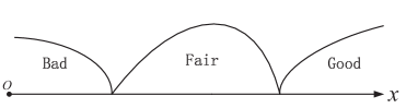
(a) Frame of discernment in Dempster-Shafer evidence theory

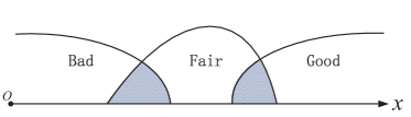
(b) Problem domain in D numbers

Figure 2: The comparison between the frame of discernment in Dempster-Shafer evidence theory and the problem domain in D numbers

If a problem domain is $\Omega=\{b_{1},b_{2},\cdots,b_{i},\cdots,b_{n}\}$, where $b_{i}\in R$ and $b_{i}\neq b_{j}$ if $i\neq j$, a special form of D numbers can be expressed by

$$\begin{array}[]{l}D(\{b_{1}\})=v_{1}\\ D(\{b_{2}\})=v_{2}\\ \cdots\qquad\cdots\\ D(\{b_{i}\})=v_{i}\\ \cdots\qquad\cdots\\ D(\{b_{n}\})=v_{n}\\ \end{array}$$ (16)

simple noted for $D=\{(b_{1},v_{1}),(b_{2},v_{2}),\cdots,(b_{i},v_{i}),\cdots,(b_{n},v_{n})\}$, where $v_{i}>0$ and $\sum\limits_{i=1}^{n}{v_{i}}\leq 1$. Some properties of D numbers are introduced as follows.

Property 1

Permutation invariability. If there are two D numbers that

$$D_{1}=\{(b_{1},v_{1}),\cdots,(b_{i},v_{i}),\cdots,(b_{n},v_{n})\}$$

and

$$D_{2}=\{(b_{n},v_{n}),\cdots,(b_{i},v_{i}),\cdots,(b_{1},v_{1})\},$$

then $D_{1}\Leftrightarrow D_{2}$.

Property 2

Let $D=\{(b_{1},v_{1}),(b_{2},v_{2}),\cdots,(b_{i},v_{i}),\cdots,(b_{n},v_{n})\}$ be a D numbers, the integration representation of $D$ is defined as

$$I(D)=\sum\limits_{i=1}^{n}{b_{i}v_{i}}$$ (17)

where $b_{i}\in R$, $v_{i}>0$ and $\sum\limits_{i=1}^{n}{v_{i}}\leq 1$.

3.2 Combination rule of D numbers

3.2.1 Relative matrix.

$n$ linguistic constants expressed in normal triangular fuzzy numbers are illustrated in Fig. 3. The area of intersection $S_{ij}$ and union $U_{ij}$ between any two triangular fuzzy numbers $L_{i}$ and $L_{j}$ can be can calculated to represent the non-exclusive degree between two D numbers. For example, the intersection $S_{12}$ and the union $U_{12}$ in Fig. 3. The non-exclusive degree $D_{ij}$ can be calculated as follows:

$$D_{ij}=\frac{S_{ij}}{U_{ij}}$$ (18)

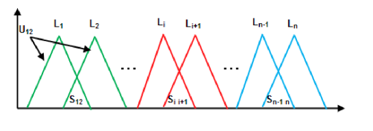
Figure 3: Four linguistic constants.

It should be emphasized that how to determine the non-exclusive degree depends on the application type. Due to the characteristic of the fuzzy numbers, we choose the area of intersection and union between two fuzzy numbers. A relative Matrix for these elements based on the non-exclusive degree can be build as below:

$$R=\left[\begin{array}[]{ccccccc}&L_{1}&L_{2}&\ldots&L_{i}&\ldots&L_{n}\\ L_{1}&1&D_{12}&\ldots&D_{1i}&\ldots&D_{1n}\\ L_{2}&D_{21}&1&\ldots&D_{2i}&\ldots&D_{2n}\\ \vdots&\vdots&\vdots&\ldots&\vdots&\ldots&\vdots\\ L_{i}&D_{i1}&D_{i2}&\ldots&1&\ldots&D_{in}\\ \vdots&\vdots&\vdots&\ldots&\vdots&\ldots&\vdots\\ L_{n}&D_{n1}&D_{n2}&\ldots&D_{ni}&\ldots&1\end{array}\right]$$ (19)

3.2.2 Exclusive coefficient.

The exclusive coefficient $\varepsilon$ is used to characterize the exclusive degree of the propositions in a assessment situation, which is got by calculating the average non-exclusive degree of these elements using the upper triangular of the relative matrix. Namely:

$$\varepsilon=\frac{\sum_{i,j=1,i\neq{j}}^{n}{D_{ij}}}{n(n-1)/2}$$ (20)

where $n$ is the number of the propositions in the assessment situation. Smaller the $\varepsilon$ is, the more exclusive the propositions of the application are. When $\varepsilon=0$, the propositions of application are completely mutually exclusive. That is, this situation is up to the requirements of the Dempster-Shafer evidence theory.

The combination rule of D numbers. Firstly, the given D numbers should be discounted by the exclusive coefficient $\varepsilon$, which can guarantee the elements in the frame of discernment $\Omega$ to be exclusive. The D numbers can be discounted as below:

$$D(A_{i})_{\varepsilon}=D(A_{i}).(1-\varepsilon)$$

$$D(\Theta)_{\varepsilon}=D(\Theta).(1-\varepsilon)+\varepsilon$$ (21)

where $A_{i}$ is the elements in $\Omega$.

Then the combination rule of D numbers based on the exclusive coefficient is illustrated as follows.

$$D(A)_{\varepsilon}=\frac{\sum_{B\cap{C}=A}{D_{1}(B)_{\varepsilon}D_{2}(C)_{\varepsilon}}}{1-k}$$ (22)

with

$$k=\sum_{B\cap{C}={\phi}}{D_{1}(B)_{\varepsilon}D_{2}(C)_{\varepsilon}}$$ (23)

where $k$ is a normalization constant, called conflict because it measures the degree of conflict between $D_{1}$ and $D_{2}$.

One should note that, if $\varepsilon=0$, i.e, the elements in the frame of discernment $\Omega$ are completely mutually exclusive, the D numbers will not be discount by the exclusive coefficient. That is, the mutually exclusive situation of D numbers is completely the same with the Dempster-Shafer evidence theory.

3.3 Decision making based on linguistic variable transformation

In this section, we propose a so called linguistic variable transformation. If the hypothesis is exclusive with each other, the LVT is degenerated to PPT in transferable belief model.

Definition 10

The transformation is determined by the area ratio of the intersection $S_{ij}$ and the corresponding linguistic variable area.

$${D_{LVT}}(A)=D(A)+D(A,B)\frac{{\frac{{{S_{AB}}}}{{{S_{A}}}}}}{{\frac{{{S_{AB}}}}{{{S_{A}}}}+\frac{{{S_{AB}}}}{{{S_{B}}}}}}$$ (24)

$${D_{LVT}}(B)=D(B)+D(A,B)\frac{{\frac{{{S_{AB}}}}{{{S_{B}}}}}}{{\frac{{{S_{AB}}}}{{{S_{A}}}}+\frac{{{S_{AB}}}}{{{S_{B}}}}}}$$ (25)

where $S_{AB}$ denotes the intersection area between linguistic variable $A$ and linguistic variable $B$. $S_{A}$ and $S_{B}$ represents the area of linguistic variable $A$ and linguistic variable $B$, respectively.

Without loss of generality, if the hypothesis is exclusive with each other, which means the intersection $S_{ij}=0$ between each linguistic variable, the discount ratio is $1:1$ in transferable belief model. It is worth noting that LVT is applicative when and only when one linguistic variable do not completely belongs to another linguistic variable. In the following part, a simple example is given to show how LVT works. Suppose the original D number is

$$\begin{array}[]{l}D(VP,P)=0.8\\ D(P)=0.2\end{array}$$

Fig. 4 shows the linguistic variable as described in Table 2.

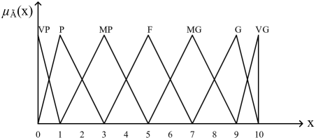
Figure 4: The linguistic variable as described in Table 2.

The areas can be obtained:

$$\begin{array}[]{l}{S_{VP,P}}=0.5\times 1\times 0.5=0.25\\ {S_{VP}}=0.5\times 1\times 1=1\\ {S_{P}}=0.5\times 3\times 1=1.5\end{array}$$

Using Eqs.(24) and (25), the final D number by LVT is calculated

$$\begin{array}[]{l}{D_{LVT}}(VP)=0.8\times\frac{{\frac{{0.25}}{1}}}{{\frac{{0.25}}{1}+\frac{{0.25}}{{1.5}}}}=0.6\\ {D_{LVT}}(P)=0.2+0.8\times\frac{{\frac{{0.25}}{{1.5}}}}{{\frac{{0.25}}{1}+\frac{{0.25}}{{1.5}}}}=0.4\end{array}$$

4 Application

To demonstrate the efficiency and practicability of the proposed method, the example illustrated in [47] is used. Suppose that a company desires to hire an engineer. After preliminary screening, three candidates $A_{1}$, $A_{2}$ and $A_{3}$ remain for further evaluation. A committee of three experts, $D_{1}$, $D_{2}$ and $D_{3}$ has been formed to conduct the interview and select the most suitable candidate. Five benefit criteria are considered:
(1) emotional steadiness ($C_{1}$)
(2) oral communication skill ($C_{2}$)
(3) personality ($C_{3}$)
(4) past experience ($C_{4}$)
(5) self-confidence ($C_{5}$)

Fig. 5 shows the hierarchical structure of the decision process. The proposed method is now applied to solve this decision problem. Then, computational procedure is summarized as follows:

Step 1: The experts use linguistic weighting variables to assess the importance of the criteria, which is shown in Table 3.

Step 2: Using the linguistic rating variables, the ratings of the three candidates by experts under all criteria is obtained as shown in Table 4.

Step 3: Convert the linguistic weighted evaluation shown in Tables 3 and 4 into triangular fuzzy numbers as shown in Table 5.

Step 4: Calculating the ratio of the intersection between the obtained triangular fuzzy number area and the single linguistic variable area to construct the D numbers in each candidate with five criteria as shown in Table 6.

Note that the non-intersecting area represents that this part may belongs to arbitrary linguistic variables, where this ratio is defined as $D(\Theta)$.

Step 5: The discounted D numbers with exclusive coefficient are aggregated by the combination rule of D numbers. The results are shown in Table 7.

Step 6: The proposed linguistic variables transformation (LVT), converted a belief function to a probability function benefited to making a decision, is used to get the final combined D number of three candidates with five criteria as shown in Table 8.

Step 7: The decision of choosing which one candidate is determined by the maximum supported degree of “$Medium~{}Good$” $MSD(MG)$. Calculate $MSD(MG)$ by the sum of “$MG$”, “$G$”, and “$VG$” of each candidate as

$$MS{D_{{A_{1}}}}(MG)={D_{{A_{1}}}}(\{MG\})+{D_{{A_{1}}}}(\{G\})+{D_{{A_{1}}}}(\{VG\})=0.9444$$

$$MS{D_{{A_{2}}}}(MG)={D_{{A_{2}}}}(\{MG\})+{D_{{A_{2}}}}(\{G\})+{D_{{A_{2}}}}(\{VG\})=0.9858$$

$$MS{D_{{A_{3}}}}(MG)={D_{{A_{3}}}}(\{MG\})+{D_{{A_{3}}}}(\{G\})+{D_{{A_{3}}}}(\{VG\})=0.9828$$

Step 8: According to the maximum supported degree of “$Medium~{}Good$”, the ranking order of the three candidates is ${A_{2}}\succ{A_{3}}\succ{A_{1}}$, where “$\succ$” represents “$better~{}than$”. Obviously, the best selection is candidate $A_{2}$.

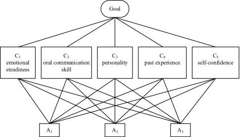
Figure 5: The hierarchical structure

Table 3: The importance weight of the criteria

	$E_{1}$	$E_{2}$	$E_{3}$
$C_{1}$	H	VH	MH
$C_{2}$	VH	VH	VH
$C_{3}$	VH	H	H
$C_{4}$	VH	VH	VH
$C_{5}$	M	MH	MH

Table 4: The ratings of the three candidates by experts under all criteria

Criteria	Candidates	Experts
		$E_{1}$	$E_{2}$	$E_{3}$
$C_{1}$	$A_{1}$	MG	G	MG
	$A_{2}$	G	G	MG
	$A_{3}$	VG	G	F
$C_{2}$	$A_{1}$	G	MG	F
	$A_{2}$	VG	VG	VG
	$A_{3}$	MG	G	VG
$C_{3}$	$A_{1}$	F	G	G
	$A_{2}$	VG	VG	G
	$A_{3}$	G	MG	VG
$C_{4}$	$A_{1}$	VG	G	VG
	$A_{2}$	VG	VG	VG
	$A_{3}$	G	VG	MG
$C_{5}$	$A_{1}$	F	F	F
	$A_{2}$	VG	MG	G
	$A_{3}$	G	G	MG

Table 5: The triangular fuzzy numbers of three candidates with five criteria

	$C_{1}$	$C_{2}$	$C_{3}$	$C_{4}$	$C_{5}$
$A_{1}$	(4.87,6.56,7.92)	(4.83,6.77,8.38)	(5.01,6.81,8.03)	(7.22,8.38,8.67)	(1.90,3.17,4.43)
$A_{2}$	(5.44,7.13,8.21)	(8.70,9.67,9.67)	(7.52,8.71,9.00)	(7.80,8.67,8.67)	(4.30,5.40,6.10)
$A_{3}$	(5.56,6.96,7.44)	(6.77,8.38,9.34)	(6.30,7.81,8.71)	(6.07,7.51,8.38)	(3.97,5.23,6.10)

Table 6: The obtained D number of three candidates with five criteria

$C_{i}$	$A_{1}$	$A_{2}$	$A_{3}$
$C_{1}$	$D(\{MP\},\{F\})=0.0015$	$D(\{F\},\{MG\})=0.2381$	$D(\{F\},\{MG\})=0.3244$
	$D(\{F\})=0.0744$	$D(\{MG\})=0.5853$	$D(\{MG\})=0.6330$
	$D(\{F\},\{MG\})=0.3279$	$D(\{MG\},\{G\})=0.1716$	$D(\{MG\},\{G\})=0.0415$
	$D(\{MG\})=0.4215$	$D(\Theta)=0.0050$	$D(\Theta)=0.0011$
	$D(\{MG\},\{G\})=0.0826$
	$D(\Theta)=0.0921$
$C_{1}$	$D(\{MP\},\{F\})=0.0021$	$D(\{MG\},\{G\})=0.0312$	$D(\{F\},\{MG\})=0.0057$
	$D(\{F\})=0.0529$	$D(\{G\})=0.3377$	$D(\{MG\})=0.1412$
	$D(\{F\},\{MG\})=0.2817$	$D(\{G\},\{VG\})=0.4032$	$D(\{MG\},\{G\})=0.3891$
	$D(\{MG\})=0.4611$	$D(\{VG\})=0.0596$	$D(\{G\})=0.3077$
	$D(\{MG\},\{G\})=0.1486$	$D(\Theta)=0.1983$	$D(\{G\},\{VG\})=0.0230$
	$D(\Theta)=0.0536$		$D(\Theta)=0.1333$
$C_{1}$	$D(\{F\})=0.0141$	$D(\{MG\})=0.4639$	$D(\{F\},\{MG\})=0.0579$
	$D(\{F\},\{MG\})=0.3310$	$D(\{MG\},\{G\})=0.4907$	$D(\{MG\})=0.3889$
	$D(\{MG\})=0.5039$	$D(\Theta)=0.0454$	$D(\{MG\},\{G\})=0.3832$
	$D(\{MG\},\{G\})=0.1091$		$D(\{G\})=0.0352$
	$D(\Theta)=0.0419$		$D(\Theta)=0.1348$
$C_{1}$	$D(\{MG\})=0.0416$	$D(\{MG\})=0.5141$	$D(\{F\},\{MG\})=0.1088$
	$D(\{MG\},\{G\})=0.6060$	$D(\{MG\},\{G\})=0.4377$	$D(\{MG\})=0.5370$
	$D(\{G\})=0.1942$	$D(\Theta)=0.0482$	$D(\{MG\},\{G\})=0.2873$
	$D(\Theta)=0.1582$		$D(\Theta)=0.0669$
$C_{1}$	$D(\{P\},\{MP\})=0.1463$	$D(\{MP\},\{F\})=0.0878$	$D(\{MP\},\{F\})=0.1528$
	$D(\{MP\})=0.5939$	$D(\{F\})=0.6235$	$D(\{F\})=0.6349$
	$D(\{MP\},\{F\})=0.2479$	$D(\{F\},\{MG\})=0.2490$	$D(\{F\},\{MG\})=0.1979$
	$D(\Theta)=0.0119$	$D(\Theta)=0.0397$	$D(\Theta)=0.0144$

Table 7: The combination of discounted D number

$A_{1}$	$A_{2}$	$A_{3}$
$D(\{P\},\{MP\})=0.00083$	$D(\{MP\},\{F\})=0.00027$	$D(\{MP\},\{F\})=0.00016$
$D(\{MP\})=0.00346$	$D(\{F\})=0.01096$	$D(\{F\})=0.01418$
$D(\{MP\},\{F\})=0.00146$	$D(\{F\},\{MG\})=0.00561$	$D(\{F\},\{MG\})=0.00569$
$D(\{F\})=0.03973$	$D(\{MG\})=0.54548$	$D(\{MG\})=0.97317$
$D(\{F\},\{MG\})=0.01988$	$D(\{MG\},\{G\})=0.05219$	$D(\{MG\},\{G\})=0.00408$
$D(\{MG\})=0.92027$	$D(\{G\})=0.38467$	$D(\{G\})=0.00265$
$D(\{MG\},\{G\})=0.01127$	$D(\{G\},\{VG\})=0.00049$	$D(\{G\},\{VG\})=0.00001$
$D(\{G\})=0.00278$	$D(\{VG\})=0.00007$	$D(\Theta)=0.00006$
$D(\Theta)=0.00032$	$D(\Theta)=0.00026$

Table 8: The final D number by linguistic variables transformation

$A_{1}$	$A_{2}$	$A_{3}$
$D(\{VP\})=0.000094$	$D(\{VP\})=0.000075$	$D(\{VP\})=0.000018$
$D(\{P\})=0.000503$	$D(\{P\})=0.000025$	$D(\{P\})=0.000006$
$D(\{MP\})=0.004567$	$D(\{MP\})=0.000153$	$D(\{MP\})=0.000084$
$D(\{F\})=0.050428$	$D(\{F\})=0.013921$	$D(\{F\})=0.017102$
$D(\{MG\})=0.935062$	$D(\{MG\})=0.570672$	$D(\{MG\})=0.977771$
$D(\{G\})=0.009252$	$D(\{G\})=0.414680$	$D(\{G\})=0.004996$
$D(\{VG\})=0.000094$	$D(\{VG\})=0.000474$	$D(\{VG\})=0.000023$

5 Conclusion

One of the assumptions to apply the Dempster-Shafer evidence evidence theory is that all the elements in the frame of discernment should be mutually exclusive. However, it is difficult to meet the requirement in the real-world applications. In this paper, a new mathematic tool to model uncertain information, called as D numbers, is used to model and combine the domain experts’ opinions under the condition that the linguistic constants are not exclusive with each other. An exclusive coefficient is proposed to discount the D numbers. After the discounted D numbers are obtained, the domain experts’ opinion can be fused based on our proposed combination rule of D numbers. It is inevitable to handle the experts’ subjective opinion, the proposed D numbers is promising methodology since it provides more flexible way than classical evidence theory to deal with uncertain. Though the D numbers theory is illustrated to handle linguistic decision making problems in this paper, the proposed theory can handle other situation when the hypothesis is not exclusive with each other. Fianlly, when the elements in the frame of discernment are mutually exclusive, D numbers theory is degenerated as classical Dempster Shafer evidence theory.

References

References

- Zadeh [1984] L. A. Zadeh, Review of a mathematical theory of evidence, AI magazine 5 (3) (1984) 81.
- Zadeh [1965] L. A. Zadeh, Fuzzy sets, Information and control 8 (3) (1965) 338–353.
- Pawlak and Skowron [2007a] Z. Pawlak, A. Skowron, Rudiments of rough sets, Information sciences 177 (1) (2007a) 3–27.
- Pawlak and Skowron [2007b] Z. Pawlak, A. Skowron, Rough sets: some extensions, Information sciences 177 (1) (2007b) 28–40.
- Dempster [1967a] A. P. Dempster, Upper and lower probabilities induced by a multivalued mapping, The annals of mathematical statistics (1967a) 325–339.
- Shafer [1976] G. Shafer, A mathematical theory of evidence, vol. 1, Princeton university press Princeton, 1976.
- Sadiq et al. [2006] R. Sadiq, Y. Kleiner, B. Rajani, Estimating risk of contaminant intrusion in water distribution networks using Dempster–Shafer theory of evidence, Civil Engineering and Environmental Systems 23 (3) (2006) 129–141.
- Huang et al. [2014] S. Huang, X. Su, Y. Hu, S. Mahadevan, Y. Deng, A new decision-making method by incomplete preferences based on evidence distance, Knowledge-Based Systems (56) (2014) 264–272.
- Denoeux and Smets [2006] T. Denoeux, P. Smets, Classification using belief functions: relationship between case-based and model-based approaches, IEEE Transactions on Systems Man and Cybernetics Part B-Cybernetics 36 (6) (2006) 1395–1406.
- Yang and Xu [2002] J.-B. Yang, D.-L. Xu, On the evidential reasoning algorithm for multiple attribute decision analysis under uncertainty, IEEE Transactions on Systems Man and Cybernetics Part A-Systems and Humans 32 (3) (2002) 289–304.
- Yang and Singh [1994] J.-B. Yang, M. G. Singh, An evidential reasoning approach for multiple-attribute decision making with uncertainty, IEEE Transactions on Systems Man and Cybernetics 24 (1) (1994) 1–18.
- Kang et al. [2012] B. Kang, Y. Deng, R. Sadiq, S. Mahadevan, Evidential cognitive maps, Knowledge-Based Systems 35 (2012) 77–86.
- Wei et al. [2013] D. Wei, X. Deng, X. Zhang, Y. Deng, S. Mahadevan, Identifying influential nodes in weighted networks based on evidence theory, Physica A: Statistical Mechanics and its Applications 392 (10) (2013) 2564–2575.
- Beynon [2002] M. Beynon, DS/AHP method: A mathematical analysis, including an understanding of uncertainty, European Journal of Operational Research 140 (1) (2002) 148–164.
- Beynon et al. [2000] M. Beynon, B. Curry, P. Morgan, The Dempster-Shafer theory of evidence: an alternative approach to multicriteria decision modelling, Omega 28 (1) (2000) 37–50.
- Beynon [2005] M. J. Beynon, A method of aggregation in DS/AHP for group decision-making with the non-equivalent importance of individuals in the group, Computers & Operations Research 32 (7) (2005) 1881–1896.
- Yao et al. [2010] S. Yao, Y.-J. Guo, W.-Q. Huang, An improved method of aggregation in DS/AHP for multi-criteria group decision-making based on distance measure, Control and Decision 25 (6) (2010) 894–898.
- Ma et al. [2013] W. Ma, W. Xiong, X. Luo, A model for decision making with missing, imprecise, and uncertain evaluations of multiple criteria, International Journal of Intelligent Systems 28 (2) (2013) 152–184.
- Ju and Wang [2012] Y. Ju, A. Wang, Emergency alternative evaluation under group decision makers: A method of incorporating DS/AHP with extended TOPSIS, Expert Systems with Applications 39 (1) (2012) 1315–1323.
- Utkin and Zhuk [2012] L. V. Utkin, Y. A. Zhuk, Combining of judgments in imprecise voting multi-criteria decision problems, International Journal of Applied Decision Sciences 5 (3) (2012) 199–214.
- Deng and Chan [2011] Y. Deng, F. T. Chan, A new fuzzy dempster MCDM method and its application in supplier selection, Expert Systems with Applications 38 (8) (2011) 9854–9861.
- Beynon [2006] M. J. Beynon, The role of the DS/AHP in identifying inter-group alliances and majority rule within group decision making, Group decision and negotiation 15 (1) (2006) 21–42.
- Deng et al. [2014a] X. Deng, Y. Hu, Y. Deng, S. Mahadevan, Supplier selection using AHP methodology extended by D numbers, Expert Systems with Applications 41 (1) (2014a) 156–167.
- Jousselme and Maupin [2012] A.-L. Jousselme, P. Maupin, Distances in evidence theory: Comprehensive survey and generalizations, International Journal of Approximate Reasoning 53 (2) (2012) 118–145.
- Deng et al. [2013] X. Deng, Q. Liu, Y. Hu, Y. Deng, TOPPER: Topology prediction of transmembrane protein based on evidential reasoning, The Scientific World Journal (2013) http://dx.doi.org/10.1155/2013/123731. Article ID 123731.
- Liu et al. [2012] J. Liu, F. T. Chan, Y. Li, Y. Zhang, Y. Deng, A new optimal consensus method with minimum cost in fuzzy group decision, Knowledge-Based Systems 35 (2012) 357–360.
- Wang et al. [2013] Y. Wang, J. Zhang, X. Chen, X. Chu, X. Yan, A spatial–temporal forensic analysis for inland–water ship collisions using AIS data, Safety Science 57 (2013) 187–202.
- Zargar et al. [2012] A. Zargar, R. Sadiq, G. Naser, F. I. Khan, N. N. Neumann, Dempster-Shafer Theory for Handling Conflict in Hydrological Data: Case of Snow Water Equivalent, Journal of Computing in Civil Engineering 26 (3) (2012) 434–447.
- Yang et al. [2011] J. Yang, H.-Z. Huang, L.-P. He, S.-P. Zhu, D. Wen, Risk evaluation in failure mode and effects analysis of aircraft turbine rotor blades using Dempster-Shafer evidence theory under uncertainty, Engineering Failure Analysis 18 (8) (2011) 2084–2092.
- Denoeux [2013] T. Denoeux, Maximum likelihood estimation from uncertain data in the belief function framework, IEEE Transactions on Knowledge and Data Engineering 25 (2013) 119–130.
- Deng et al. [2014b] X. Deng, Y. Hu, Y. Deng, S. Mahadevan, Environmental impact assessment based on D numbers, Expert Systems with Applications 41 (2) (2014b) 635–643.
- Deng [2012] Y. Deng, D Numbers: Theory and Applications, Journal of Information and Computational Science 9 (9) (2012) 2421–2428.
- Deng et al. [2014c] X. Deng, Y. Hu, Y. Deng, S. Mahadevan, Supplier selection using AHP methodology extended by D numbers, Expert Systems with Applications 41 (1) (2014c) 156–167.
- Deng et al. [2014d] X. Deng, Y. Hu, Y. Deng, Bridge condition assessment using D numbers, The Scientific World Journal 2014 (2014d) Article ID 358057, 11 pages, doi:10.1155/2014/358057.
- Deng et al. [2012] Y. Deng, Y. Chen, Y. Zhang, S. Mahadevan, Fuzzy Dijkstra algorithm for shortest path problem under uncertain environment, Applied Soft Computing 12 (3) (2012) 1231–1237.
- Zhang et al. [2013] X. Zhang, Y. Deng, F. T. Chan, P. Xu, S. Mahadevan, Y. Hu, IFSJSP: A novel methodology for the Job-Shop Scheduling Problem based on intuitionistic fuzzy sets, International Journal of Production Research 51 (17) (2013) 5100–5119.
- Zadeh [1975a] L. A. Zadeh, The concept of a linguistic variable and its application to approximate reasoning I, Information sciences 8 (3) (1975a) 199–249.
- Zadeh [1975b] L. A. Zadeh, The concept of a linguistic variable and its application to approximate reasoning II, Information sciences 8 (4) (1975b) 301–357.
- Zadeh [1975c] L. A. Zadeh, The concept of a linguistic variable and its application to approximate reasoning-III, Information sciences 9 (1) (1975c) 43–80.
- Zimmermann [1991] H. Zimmermann, Fuzzy set theory and its applications, Kluwer, Boston, 1991.
- Dempster [1967b] A. P. Dempster, Upper and lower probabilities induced by a multi-valued mapping, Annals of Mathematics and Statistics 38 (1967b) 325–339.
- Halpern and Fagin [1992] J. Y. Halpern, R. Fagin, Two views of belief: belief as generalized probability and belief as evidence, Artificial Intelligence 54 (3) (1992) 275–317.
- Smets and Kennes [1994] P. Smets, R. Kennes, The transferable belief model, Artificial intelligence 66 (2) (1994) 191–234.
- Chen et al. [2013] S. Chen, Y. Deng, J. Wu, Fuzzy sensor fusion based on evidence theory and its application, Applied Artificial Intelligence 27 (3) (2013) 235–248.
- Du et al. [2012] H. L. Du, F. Lv, N. Du, A Method of Multi-Classifier Combination Based on Dempster-Shafer Evidence Theory and the Application in the Fault Diagnosis, Advanced Materials Research 490 (2012) 1402–1406.
- Díaz-Más et al. [2012] L. Díaz-Más, F. J. Madrid-Cuevas, R. Muñoz-Salinas, A. Carmona-Poyato, R. Medina-Carnicer, An octree-based method for shape from inconsistent silhouettes, Pattern Recognition 45 (9) (2012) 3245–3255.
- Chen [2000] C.-T. Chen, Extensions of the TOPSIS for group decision-making under fuzzy environment, Fuzzy sets and systems 114 (1) (2000) 1–9.