Hydrogenation-induced ferromagnetism on graphite surfaces

Abstract

We calculate the electronic structure and magnetic properties of hydrogenated graphite surfaces using van der Waals density functional theory (DFT) and model Hamiltonians. We find, as previously reported, that the interaction between hydrogen atoms on graphene favors adsorption on different sublattices along with an antiferromagnetic coupling of the induced magnetic moments. On the contrary, when hydrogenation takes place on the surface of graphene multilayers or graphite (Bernal stacking), the interaction between hydrogen atoms competes with the different adsorption energies of the two sublattices. This competition may result in all hydrogen atoms adsorbed on the same sublattice and, thereby, in a ferromagnetic state for low concentrations. Based on the exchange couplings obtained from the DFT calculations, we have also evaluated the Curie temperature by mapping this system onto an Ising-like model with randomly located spins. Remarkably, the long-range nature of the magnetic coupling in these systems makes the Curie temperature size dependent and larger than room temperature for typical concentrations and sizes.

I Introduction

Hydrogenation of carbon nanostructures is recently attracting a lot of interest as a methodology that allows for the tuning of their mechanical, electronic, and magnetic properties. In contrast to direct manipulation of the carbon atoms, e.g., creating vacancies Gómez-Navarro et al. (2005); Ugeda et al. (2010) or reshaping edges Jia et al. (2009), hydrogenation can effectively affect the electronic properties in a similar manner with the advantage that is a reversible process. For instance, hydrogenation of graphene was found, both theoretically and experimentally, to be a way to turn graphene from a gapless semiconductor into a gapful one with a tunable band gap (Elias et al., 2009; Sessi et al., 2009; Haberer et al., 2010; Yang et al., 2010; Balog et al., 2010). It has also been predicted that partial hydrogenation may induce interesting magnetic properties in graphene with potential applications in spintronics (Soriano et al., 2010). For instance, H-induced ferromagnetism is expected under some very particular conditions Zhou et al. (2009). Recent experiments on hydrogenated or fluorinated graphene, however, do not show evidence of ferromagnetism, but rather of paramagnetic behaviour Sepioni et al. (2010); Nair et al. (2012); McCreary et al. (2012).

Many calculations related to the adsorption of H atoms on graphene have been reported in the literature, mostly being based on first-principles or density functional theory (DFT). All the reports coincide in that adsorptive carbon atoms are puckered and, most importantly, that the covalent bond between carbon and H leads to magnetic moments on neighboring carbon atoms totalling 1.0 $\mu_{{\rm B}}$(Lehtinen et al., 2003; Boukhvalov et al., 2008; Casolo et al., 2009; Soriano et al., 2011). Such spin polarization is mainly localized around the adsorptive carbon atom. The magnetic coupling between H atoms adsorbed on graphene has also been studied and basically follows the rules expected from Lieb’s theorem Lieb (1989). Graphene is a single layer of carbon atoms bonded together in a bipartite honeycomb structure. It is thus formed by two interpenetrating triangular sublattices, A and B, such that the nearest neighbors of an atom A belong to the sublattice B and vice versa (Saito et al., 1998). Three different magnetic states can be triggered by a H pair, namely, non-magnetic, ferromagnetic, and antiferromagnetic. The most energetically stable configuration corresponds to having both H atoms adsorbed on two nearest-neighbor carbon atoms, leading to a non-magnetic ground state (Boukhvalov et al., 2008; Casolo et al., 2009; Soriano et al., 2010, 2011). When both H atoms are on the same sublattice they are coupled ferromagnetically with total spin $S=1$. When the pair of H atoms is adsorbed on different sublattices, but sufficiently far away from each other, they induce magnetic moments that couple antiferromagnetically ($S=0$) Soriano et al. (2010). As we show here, for similar distances between the H atoms the ferromagnetic coupling is always favored over the antiferromagnetic one. Previous calculations for vacancy-induced magnetism in graphene have shown similar results as long as the vacancies do not reconstruct (Yazyev and Helm, 2007; Palacios et al., 2008).

Concerning graphite, a few experimental studies, not free from controversy, have reported changes in the magnetic properties produced by irradiation of the graphite sample. The results show that graphite can become ferromagnetic at room temperature out of an originally non-magnetic sample. The ferromagnetic state appears at low concentration of the impurities induced by the irradiation and is independent of the irradiation ion type used (Esquinazi et al., 2003; Ramos et al., 2010). Unlike the case of graphene, not many theoretical studies have been reported in the literature on the magnetic properties of irradiated or hydrogenated graphite. Yazyev(Yazyev, 2008), for instance, has studied the magnetic properties of hydrogenated graphite using a combination of mean-field Hubbard model and first-principles calculations. He obtained, as expected, that the sublattices are inequivalent (approx. 0.16 eV) for hydrogenation in bulk. Graphite is a semi-metal composed of stacked graphene layers. The typical Bernal stacking of these planes effectively breaks sublattice symmetry: A atoms (for instance) are located exactly above and below the atoms of neighboring planes ($\alpha$ atoms from now on) while B atoms are located at the center of the hexagonal rings of the neighboring planes ($\beta$ atoms)(Pauling, 1960).

Here we are concerned with hydrogenation of the surface of graphite. First, through DFT calculations, we revisit the energetics of a H pair on graphene. We confirm previous results and, by considering very large supercells, we find the expected antiferromagnetic state when H atoms are adsorbed sufficiently far apart from each other on different sublattices. Next we present results for the adsorption energies on different sublattices for bilayer and multilayer graphene. Both sets of results are then combined to estimate the maximum average concentration for which all H atoms may occupy the same sublattice and, thereby, will be coupled ferromagnetically. We also compute the exchange coupling constants as a function of the relative distance between H atoms. Finally, we present a study of the Curie temperature in this system based on a Ising model constructed with the DFT coupling constants. Our results support the possible existence of surface sublattice-polarized hydrogenation and concomitant ferromagnetism.

II Atomic, electronic, and magnetic structure of H atoms on graphene and graphene multilayers

II.1 Computational Details

Our calculations are based on the DFT framework(Hohenberg and Kohn, 1964; Kohn and Sham, 1965) as implemented in the SIESTA code (Ordejón et al., 1996; Soler et al., 2002). We are mostly interested here in multilayer graphene and graphite where dispersion (van der Waals) forces due to long-range electron correlation effects play a key role in the binding of the graphene layers. Therefore we use the exchange and correlation nonlocal van der Waals density functional (vdW-DF) of Dion et al. (Dion et al., 2004) as implemented by Román-Pérez and Soler (Román-Pérez and Soler, 2009; Kong et al., 2009). To describe the interaction between the valence and core electrons we used norm-conserved Troullier-Martins pseudopotentials (Troullier and Martins, 1991). To expand the wavefunctions of the valence electrons a double-$\zeta$ plus polarization (DZP) basis set was used (Junquera et al., 2001). We experimented with a variety of basis sets and found that, for both graphene and graphite, the DZP produced high-quality results. The plane-wave cutoff energy for the wavefunctions was set to 500 Ryd. For the Brillouin zone sampling we use $4\times 4\times 2$ Monkhorst-Pack (MP) $k$-mesh for the largest $12\times 12\times 1$ single-layer and for the bilayer graphene supercells. We have also checked that the results are well converged with respect to the real space grid. Regarding the atomic structure, the atoms are allowed to relax down to a force tolerance of 0.005 eV/Å. All supercells are large enough to ensure that the vacuum space is at least 25 Å so that the interaction between functionalized graphene layers and their periodic images is safely avoided. Spin polarization was included in the calculations because, as discussed in the introduction, hydrogenation is known to induce magnetism in single-layer and, possibly, also in bilayer and multilayer graphene.

II.2 Preliminary checks

We begin our study by optimizing the geometric structures of the monolayer, bilayer graphene, and graphite in their natural nonmagnetic state. The C-C bond lengths and cell parameters ($a$ and $c$) and the interlayer distances between the layers ($d$) are listed in Table (1). The accuracy of our procedure is very satisfactory when these magnitudes are contrasted against experimental values. For completeness, we present the atomic structures of single-layer and bilayer graphene in Fig. 1. Different colors are used to stress different sublattices.

Table 1: Atomic structure parameters of monolayer, bilayer graphene, and graphite.

	C-C bond (Å)	$a$ (Å)	$c$ (Å)	$d$ (Å)
Graphene	1.419	2.458	25	-
Bilayer	1.420	2.459	25	3.353
Graphite	1.417	2.455	6.709	3.354
Experimental		2.456 (Sands, 1994)	6.696 (Sands, 1994)

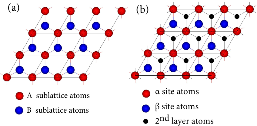
Figure 1: (Color online). Atomic structure of (a) single-layer and (b) bilayer graphene for a $3\times 3\times 1$ supercell.

In Fig. 2 we show the electronic band structure for monolayer, bilayer, five-layer graphene, and graphite along the high-symmetry points M$\Gamma$KM. The well-known case of graphene is shown in Fig. 2(a), being the result similar to that found by many others (see, for instance Ref. (Wallace, 1947; McClure, 1957; Reich et al., 2002)). Since there are two basis atoms in graphene there is one pair of $\pi\pi^{\ast}$ bands of $p_{z}$ character, which are degenerate at the K-point or Dirac Point, coinciding with the Fermi level. We have considered bilayer graphene in Bernal stacking, as for a typical graphite arrangement. Since the basis consists now of four atoms, there are two pairs of $\pi\pi^{\ast}$ bands and there are four sets of $p_{z}$-derived bands close to the K-point as shown in Fig. 2(b). Due to the interaction between the graphene layers these bands split apart. Consistent with previous theoretical works (Latil and Henrard, 2006; Min et al., 2007), we find that, similar to monolayer graphene, the bilayer graphene is also a zero-gap semiconductor with a pair of the $\pi\pi^{\ast}$ bands being degenerate at the K-point. On the other hand, there is an energy gap of 0.8 eV between the other pair of $\pi\pi^{\ast}$ bands. The band structure for five-layer graphene is shown in Fig. 2(c) which already anticipates the characteristic band structure of graphite. For instance, at the $\Gamma$ point, five bands closely packed in energy manifest the emerging dispersion stemming from the perpendicular interlayer coupling. Finally, the bands of graphite are shown in Fig. 2(d). The results are also in agreement with previous works (see, e.g., Ref. Tatar and Rabii, 1982), exhibiting a bandwith of 1.41 eV at the K-point(Ahuja et al., 1997).

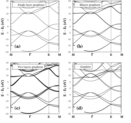
Figure 2: Electronic band structure of monolayer, bilayer, five-layer graphene, and graphite calculated with a $100\times 100\times 2$ MP-grid for a $1\times 1\times 1$ supercell.

II.3 Hydrogen atoms on monolayer graphene

II.3.1 One hydrogen atom

We revisit now, for the sake of completeness, the atomic, electronic, and magnetic structure changes induced on monolayer graphene by the adsorption of a single H atom. In Fig. 3 we present a view of the atomic structure resulting after the adsorption. This can only occur when the substrate is allowed to relax. In the stable configuration the H atom is covalently bonded to one carbon atom and is located right above this atom, as shown in Fig. 3(a). The carbon atom in the adsorption site extrudes out of the graphene plane, displaying the typical $sp^{3}$ hybridization to form the $\sigma$ C-H bond [see Fig. 3(b)]. For all supercell sizes we found that the bond lengths between the adsorptive carbon atom and its nearest neighbors increase up to 1.50Å (which is to be compared to the bond length in graphene of 1.42Å). The other bond lengths are practically unaffected and the C-H distance is always found to be 1.13Å, regardless of the supercell size. Table 2 contains a detailed account of our results compared to those found in the literature for this system.

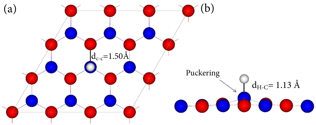
Figure 3: (Color online). Atomic structure of H on graphene. (a) Top and (b) side view for a $3\times 3\times 1$ supercell.

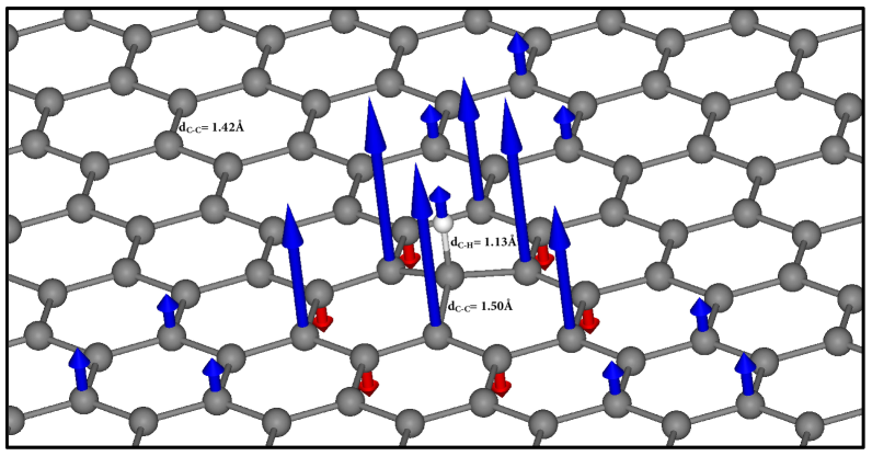
Figure 4: (Color online). Relaxed atomic structure and spin polarization around an adsorbed H atom. Magnetic moments with opposite orientations are depicted by blue and red arrows for clarity.

The adsorption energy $E_{a}$ for a H atom on graphene is calculated as usual

$$E_{a}=E_{\rm graphene+H}-(E_{\rm graphene}+E_{\rm H})$$ (1)

where $E_{\rm graphene+H}$ denotes the total energy of the complete system and $E_{\rm graphene}$ and $E_{\rm H}$ denote the energies of the isolated graphene and H atom, respectively. We have found that the binding energy between the H atom and a graphene monolayer increases with increasing supercell size. A linear fit as a function of the inverse supercell size can be done for the calculated points which shows that the adsorption energy is about -0.98 eV in the limit of zero concentration of H atoms (infinite supercell size). Obviously, for a given supercell size, the binding energy of the H atom sublattice A is equal to the binding energy of the H atom on sublattice B $[E_{a}({\rm A})=E_{a}({\rm B})]$.

Table 2: Equilibrium height of the adsorptive carbon atom above the surface $(d_{puck})$ and adsorption energies $(E_{a})$ for different supercell sizes and corresponding H concentration $C$. All the carbon atoms are allowed to relax along with the H atom.

Unit cell	$C$	$d_{puck}$ (Å)	$d_{puck}$ (Å)	$E_{a}$ (eV)	$E_{a}$(eV)
		this work	other works	this work	other works
$2\times 2$	0.125	0.359	0.36 (Sha and Jackson, 2002), 0.36 (Casolo et al., 2009), 0.36 (Ivanovskaya et al., 2010)	-0.909	-0.67 (Sha and Jackson, 2002), -0.75 (Casolo et al., 2009), -0.83 (Sljivancanin et al., 2009), -0.85 (Ivanovskaya et al., 2010)
$3\times 3$	0.056	0.476	0.41 (Kerwin and Jackson, 2008), 0.42 (Casolo et al., 2009), 0.51 (Ivanovskaya et al., 2010)	-0.915	-0.76 (Kerwin and Jackson, 2008), -0.77 (Casolo et al., 2009), -0.84 (Ivanovskaya et al., 2010)
$4\times 4$	0.031	0.485	0.48 (Casolo et al., 2009), 0.49 (Denis and Iribarne, 2009), 0.58 (Ivanovskaya et al., 2010)	-0.946	-0.76 (Duplock et al., 2004), -0.85 (Hornekær et al., 2006), -0.79 (Casolo et al., 2009), -0.89 (Denis and Iribarne, 2009), -0.89 (Ivanovskaya et al., 2010)
$5\times 5$	0.020	0.500	0.59 (Casolo et al., 2009), 0.63 (Ivanovskaya et al., 2010)	-0.950	-0.82 (Chen et al., 2007), -0.84 (Casolo et al., 2009), -0.94 (Ivanovskaya et al., 2010)
$6\times 6$	0.014	0.531	0.66 (Ivanovskaya et al., 2010)	-0.956	-0.96 (Ivanovskaya et al., 2010)
$\infty\times\infty$	0.0			-0.98

In agreement with previous studies we also find that the adsorption of H leads to the appearance of a staggered magnetization on neighbouring carbon atoms amounting to exactly 1$\mu_{\rm B}$/cell. Such spin density is mainly localized around the adsorptive carbon atom as shown in Fig. 4. In Fig. 5 we show the total density of states (DOS) for the $6\times 6$ H-graphene equilibrium structure. The H adsorption causes the appearance of peak in the DOS at the Fermi level which spin-splits due to electron-electron interactions. Remarkably, this result is compatible with Lieb’s theorem for the Hubbard model on bipartite lattices Lieb (1989). According to such theorem, the removal of a single site in the bipartite lattice should give rise to a ground state with $S=1/2$. The covalent bond between the H atom and the C atom underneath effectively suppresses the “site” (the $p_{z}$ orbital), creating a vacancy in the underlying low-energy Hamiltonian. It is worth noticing how this result contrasts with that obtained for a vacancy. As discussed in Ref. Palacios and Ynduráin, 2012, vacancies could in principle give rise to similar magnetic states. The difference with respect to the case of H adsorption is that vacancies tend to reconstruct and the magnetic moment generated actually vanishes for low concentrations.

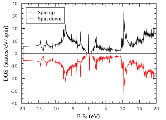
Figure 5: (Color online). Total density of states for a H atom on single-layer graphene calculated with a $6\times 6\times 1$ supercell.

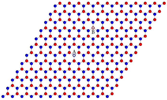
Figure 6: Atomic view of a pair of H atoms on a graphene monolayer for a $12\times 12\times 1$ supercell.

II.3.2 Two hydrogen atoms

To investigate the electronic and magnetic structure induced on graphene by two adsorbed H atoms we need to use a $12\times 12\times 1$ supercell. Figure 6 shows an example and illustrates the required size of the supercell. The use of such a large supercell is essential in order to minimize the influence of neighboring supercells on the pair-wise properties due to the relative long-range interaction between the magnetic clouds induced by the H atoms. The relative extension of the magnetic clouds with respect to the supercell size is illustrated in Figs. 7(a) and (b). Test calculations show that using larger supercells essentially gives similar results. We calculate the energetics for the two fundamentally different adsorption configurations. One in which the two H atoms are sitting on the same sublattice (AA) and the other where they are sitting on different sublattices (AB). The formation or adsorption energies for pairs of H atoms at various relative distances for some AA and AB configurations are shown in Fig. 8. (In order to see the influence of the H atoms on each other, we have subtracted twice the adsorption energy of single H atom.) We have not explored all possibilities, showing only some representative ones. Since the magnetic cloud or localized state associated to each H atom is not isotropic, an angular dependence is expected. The overall result remains valid though.

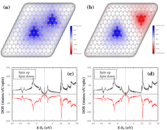
Figure 7: (Color online). Spin density (blue indicates up and red down) and spin-resolved total DOS for graphene monolayer with 2 H atoms sitting on AA [(a) and (c), respectively] and AB [(b) and (d), respectively] sublattices at far distances calculated with a $4\times 4\times 2$ MP-grid for a $12\times 12\times 1$ supercell.

First, we can see that the “interaction” energy between atoms is always negative, i.e., the H atoms “attract” each other regardless of the relative adsorption sublattices. The energy gain is the largest by placing the atoms near each other (barely noticeable for the AA cases, but clearly appreciable below 1 nm for the AB ones). This can be understood in simple terms by noticing that the H adsorption creates a localized state at the Fermi energy occupied by a single electron. When two states are created on different sublattices, these hybridize creating a bonding state that is now occupied by the two electrons forming a singlet statePalacios et al. (2008). This is essentially the reason why magnetic solutions only appear at long distances in the AB cases. As Fig. 6 shows, only for the longest possible calculated distance the H atoms retain their magnetic clouds. There the coupling is antiferromagnetic ($S=0$), as expected from Lieb’s theorem. Figures 7(b) and (d) show the spin-density and the spin-resolved DOS, respectively, in this case. The latter exhibits magnetic splitting near the Fermi energy although the DOS for both spin species are identical. On the contrary, when both atoms are on the same sublattice (AA cases) the solution is always ferromagnetic ($S=1$) regardless of distance [see Figs. 7(a) and (c)], but the energy gain with decreasing distance is very small since the localized states induced by the H atoms belong to the same sublattice and cannot hybridize.

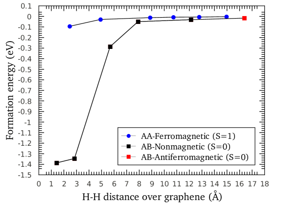
Figure 8: (Color online). Total energy for a pair of H atoms on a graphene monolayer ($12\times 12\times 1$ supercell) relative to twice the adsorption energy of a single atom. Both AA and AB cases are shown.

II.4 Hydrogen atoms on bilayer graphene

II.4.1 One hydrogen atom

The main focus of this work is actually to elucidate how the interactions of the graphene layers underlying the surface monolayer that hosts the adsorbed H atoms changes the well-established results presented in previous section. As we know, the most stable structure for bilayer graphene, multilayer graphene, and bulk graphite consists of stacked graphene monolayers following what is called Bernal stacking. In Fig. 9 we present a top view of the obtained atomic structure for the adsorption of a single H atom on a graphene bilayer. Here the upper layer is allowed to relax while the carbon atoms in the lower layer were fixed at their equilibrium position. The adsorption geometry of a H atom on a bilayer graphene surface is very similar to that for graphene monolayer. Due to the interaction between layers, however, in the bilayer graphene case (and surface graphite as shown below) the sublattices are not equivalent which translates into different adsorption energies $[E_{a}(\alpha)>E_{a}(\beta)]$. (In order to make clear that the surface sublattices are not equivalent anymore, we change the labels A and B to $\alpha$ and $\beta$ from now on.) In Fig. 10 we show the H adsorption energy difference between $\alpha$ and $\beta$ sites [$\Delta E=E_{a}(\alpha)-E_{a}(\beta)$] for different supercell sizes of the graphene bilayer. $\Delta E$ increases linearly with the supercell size, extrapolating to $\approx 85$ meV for infinitely large supercells. Importantly, the induced magnetic moment is not affected by the presence of the second graphene layer.

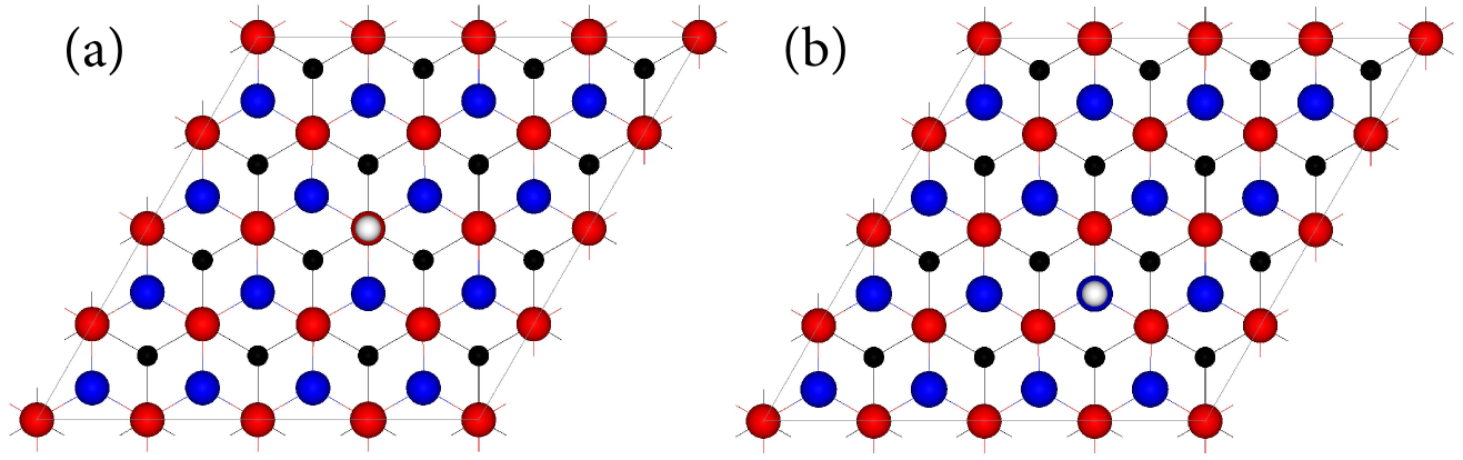
Figure 9: (Color online). Top view of the atomic structure of H on bilayer graphene for (a) $\alpha$ and (b) $\beta$ sites on a $4\times 4\times 1$ supercell.

Figure 10: (Color online). Adsorption energy difference between the two sites ($\alpha$ and $\beta$) of bilayer graphene against different cell sizes.

II.4.2 Two hydrogen atoms

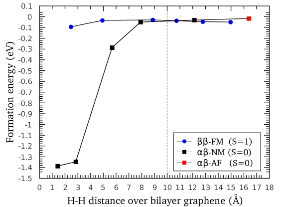
Figure 11: (Color online). Total energy for two H atoms on bilayer graphene as a function of distance.

As shown in previous sections, to properly investigate the interaction between two adsorbed H atoms, one requires very large supercells. A similar study in the bilayer case is computationally prohibited. Here we adopt a different approach. We assume that the attractive interaction between H atoms is not affected by the underlying graphene layer. This is not a strong assumption since the interaction between layers is mainly of van der Waals type while the origin of the magnetic structure changes induced on graphene by the adsorbed H are of kinetic and exchange type. We now simply shift the AA pair energy shown in Fig. 8 by the energy difference between $\alpha$ and $\beta$ adsorption sites, $\Delta E$. There are two possibilities here. One is to use the value of $\Delta E$ obtained in the limit of infinitely large supercells. The other is to use a value of $\Delta E$ that changes with the distance between H atoms. This can be estimated from the calculation for a given supercell size that approximately corresponds to such distance. Either choice obviously favors adsorption on the same sublattice ($\beta$ in this case) when the H atoms are sufficiently far apart and the intra-layer interactions are weakened. There are not significant differences between both choices and the result for the second one is shown in Fig. 11. As can be seen, the pairs of H atoms prefer to sit on the same sublattice for distances longer that $\approx 1$ nm, thus favouring a ferromagnetic state on the surface layer for a maximum coverage $C$ of around 0.05.

We note that, although the thermodynamically most stable situation is when H atoms approach one another forming pairs or clusters, the attraction between H atoms may be counteracted by the diffusion barriers, particularly at low temperaturesSljivancanin et al. (2009). Understanding the dynamics resulting from diffusion processes (and desorption ones for that matter) is of great importance to determine actual hydrogenation patterns, but this lies beyond the scope of this work. Kinetic Monte Carlo studies have been recently carried outMohammed-thesis , indicating that, since desorption rates turn out to be smaller than diffusion ones, metastable states where all H atoms stay, at least temporarily, adsorbed on the same sublattice are possible.

II.5 Hydrogen atoms on the surface of graphite

We have mentioned in passing that the magnetic moment induced in a single graphene monolayer by the H adsorption survives when a second layer is added to form a bilayer. This is result is not necessarily obvious, neither is the fact that H adsorbed on a graphite surface may induce a magnetic moment as well. As discussed in Ref. Palacios and Ynduráin (2012), vacancies tend to loose the magnetic moment because the electron-hole symmetry is severely broken and the localized state hosting the unpaired electron is not exactly placed at the Fermi energy. A similar effect could take place here. To discard this possibility we have evaluated the atomic and magnetic structures of a H atom adsorbed on graphite (represented by up to a five-layer graphene structure). In Fig. 12 we present the atomic structure determined after the adsorption of a H atom on the surface. Here, also, the upper layer is allowed to relax while the carbon atoms in the underlying layers were fixed at their equilibrium position. The adsorption of the H atom leads to the formation of a spin density on neighboring carbon atoms, again amounting to exactly 1$\mu_{\rm B}$/cell. Such spin density is mainly localized on the adsorptive layer, as shown in Fig. 12. Due to the stacking order in the multi-layer graphene structure, the sublattices are, again, inequivalent $[E_{a}(\alpha)>E_{a}(\beta)]$ for adsorption. In Table (3) we show the adsorption energy difference $\Delta E$ for a $5\times 5$ supercell size against different numbers of graphene layers. This converges very quickly with the number of layers so that the results obtained in previous section remain valid here: H atoms adsorbed on a graphite surface prefer to locate themselves on the same sublattice when sufficiently far apart from each other and induce a ferromagnetic state on the surface. The Curie temperature of this novel ferromagnet is analysed in the following section.

Table 3: Energy difference $(\Delta E)$ between $\alpha$ and $\beta$ adsorption sites for a $5\times 5$ supercell size against different numbers of graphene layers.

No. of layers	$\Delta E=E_{a}({\alpha})-E_{a}({\beta}$) (eV)
$1$	0.00000
$2$	0.03930
$3$	0.03798
$4$	0.03866
$5$	0.03857
$6$	0.03871

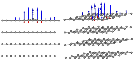
Figure 12: (Color online). Relaxed atomic structure and spin polarization around an adsorbed H atom at $\beta$ site on a 4-layer graphene surface. Magnetic moments are depicted by blue(red) arrows for spin-up(spin-down) for clarity.

III Curie Temperature

Our results show that the adsorption of H atoms on a graphite surface may induce, at low concentrations, ferromagnetically coupled spin densities distributed around the adsorbed H atoms. In the diluted regime, the extension of the polarization cloud may be considered small compared to the mean distance between H atoms; therefore, to study the collective magnetic properties of the system we will use the following Ising-like model Hamiltonian:

$$H=-\frac{1}{2}\sum_{ij}J_{ij}p_{i}S_{i}p_{j}S_{j},$$ (2)

where $S_{i}$ and $S_{j}$ are two discrete spin variables ($\pm 1$) at sites $i$ and $j$ of a given sublattice (say $\beta$) of the graphite surface. The random variables $p_{i}$ and $p_{j}$ represent the occupation of one carbon atom with a H atom. These can take the values 1 (occupied) or 0 (unoccupied). These discrete random variables are drawn from a probability density function:

$$\rho(p)=(1-c)\delta(p)+c\delta(p-1),$$ (3)

where $c$ in $[0,1]$ is related to the graphene lattice coverage by $C=c/2$. The maximum coverage in our case is thus $C=0.5$ although, as explained above, it is only meaningful for $C<0.05$. The adimensional concentration parameter $c$ defines a mean distance between H atoms $\ell=\frac{1}{\sqrt{c}}$ in units of the lattice parameter $a$. $J_{ij}$ is the magnetic coupling constant between two magnetic moments at sites $i$ and $j$. The coupling constant is defined as the total energy difference between the antiparallel (AFM) and parallel (FM) alignment of an AA pair:

$$J_{ij}=(E^{\rm FM})_{ij}-(E^{\rm AFM})_{ij}.$$ (4)

In Fig. 13 we show he magnetic coupling $J_{ij}$ as obtained from our DFT calculations in the configurations shown in Fig. 8. The exchange energy presents a slow linear decrease with the inverse of the H-H pair separation $J_{ij}=\frac{J_{0}a}{r_{ij}}$ where $J_{0}=0.0576$ eVDani , and $r_{ij}$ is the distance between H atoms at sites $i$ and $j$. As expected, it extrapolates to 0 eV in the infinite separation limit.

Figure 13: (Color online). Exchange energy for a pair of H atoms adsorbed on the same sublattice .

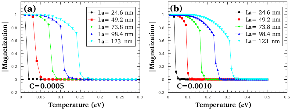
Figure 14: (Color online). Absolute magnetization per spin for supercells sizes in the range $L=24.6$ nm ($L=100$ supercell units) and 123 nm ($L=500$ supercell units), using concentrations (a) $C=0.0005$ and (b) 0.0010.

To study the magnetic ordering in this system we have used a Monte Carlo (MC) algorithm(Matsumoto et al., 2001). We have simulated very diluted triangular lattices with $L\times L$ cells with $L$ in the range $L=80-1280$. Considering that a $1/r$ coupling has always longer range than the size of the system, we have decided to apply open boundary conditions. To make contact with realistic experimental realizationsbrihuega , we have performed simulations at very low concentrations $C=0.0005,0.0006,0.0007,0.0008,0.0009$ and $0.0010$ ($C=1$ means full coverage of the graphite surface with H atoms). Note also that our simulations are performed in the range $\frac{L}{\ell}\gg 1$. The thermal averaging took 50000 MC measurements, after allowing 1000 steps for thermalization. Average over 50 random realizations of the H distribution was taken.

In Fig. 14 we show the thermal average of the magnetization absolute value $|M|$ for two concentrations ($C=0.0005$ and $C=0.0010$) and cell sizes of $L=24.6$ nm ($L=100$ supercell units), 49.2 nm, 73.8 nm, 98.4 nm, and 123 nm ($L=500$ supercell units). The abrupt supression of $|M|$ signals the approximate value of the ordering or Curie temperature $T_{\rm C}$. However, this ordering temperature seems to increase with the system size. In the thermodynamic limit this behavior extrapolates to an infinite value (i.e., a finite magnetization at any finite temperature).

We discuss now that this is an intrinsic property of the system, consequence of the long-range coupling between the induced magnetic moments. To study this we compute the Binder cumulant, used conventionally for an accurate determination of the critical temperature in MC simulations of statistical systems. The Binder cumulant is the fourth order cumulant of the order parameter distribution (Binder, 1981, 1981), which is defined as

$$U_{L}(T)=\frac{1}{2}\biggl{[}3-\frac{\langle\bar{M}^{4}\rangle}{\langle\bar{M}^{2}\rangle^{2}}\biggl{]},$$ (5)

where $\langle\bar{M}^{2}\rangle$ and $\langle\bar{M}^{4}\rangle$ are the second and fourth moments of the magnetization distribution, with the brackets $\langle...\rangle$ and the bar denoting thermal and sample averaging.

The finite-size scaling argument states that, close to a critical point, a thermal average of a generic quantity scales as

$$\langle O\rangle=L^{\mu}g_{O}(L/\xi),$$ (6)

where $L$ is the system size, $\mu$ a critical exponent, and $\xi$ is the temperature dependent correlation length which can be considered adimensional or in units of $a$. Close to the critical point, it scales as $\xi(T)\sim(T-T_{\rm C})^{-\nu}$ . It is well known that several physical properties have important finite size corrections which makes the determination of $T_{\rm C}$ difficult. However, if we specifically consider the scaling of the moments of the order parameter:

$$\langle M^{2n}\rangle=L^{{2n\beta}{\nu}}g_{M^{2n}}(L/\xi)$$ (7)

and substitute in the Binder parameter expression of Eq. 5 we get $U_{L}(T)=U(L/\xi(T))$, which is size independent at the critical point. At large temperatures the histogram of the magnetization is expected to be a Gaussian distribution and therefore $U_{L}(T\rightarrow\infty)=0$. On the other hand, in the zero temperature limit, the magnetization distribution function reduces to two delta peaks at opposite values of the saturation magnetization and hence $U_{L}(T\rightarrow 0)=1$. If a system has a well-defined second order phase transition at a finite temperature, the finite-size analysis of the Binder parameter $U_{L}(T)$ will show a family of decreasing functions of the temperature, all of them crossing, to a very good approximation, at $T_{\rm C}$.

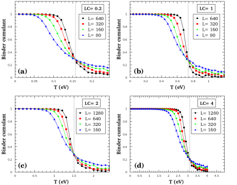
Figure 15: (Color online). Fourth-order cumulant for supercells sizes in the range $L=24.6$ nm ($L=100$ supercell units), and 123 nm ($L=500$ supercell units), using concentrations (a)$C=0.0005$, and (b) 0.0010

In our case the Binder cumulant curves do not cross at a given point (see Fig. 15) which makes it impossible to define a critical temperature. However, we have realized that if we plot the Binder cumulant against the temperature for each value of the product of the size and the concentration $LC$, then we obtain a crossing point (see Fig. 16). From this we obtain a relation between the Curie temperature $T_{\rm C}$ and $LC$ (see Fig. 17):

$$T_{\rm C}=(0.77\pm 0.01)LC\hskip 28.45274pt({\rm eV})$$ (8)

Figure 16: (Color online). Fourth-order cumulant for (a) $LC=$ 0.2, (b)$LC=$ 1.0, (c)$LC=$ 2.0, and (d)$LC=$ 4, using supercell sizes$L=$ 80, 160, 320, 460, and 1280.

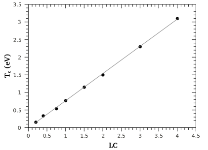
Figure 17: Critical temperature against LC.

Strictly speaking the concept of Curie temperature should be used with caution since the ordering temperature in the thermodynamic limit is not well-defined in this model. However, our numerical simulations show clearly a measurable ordering temperature in any finite lattice. The expression (8) and the Binder cumulant analysis of Figs. 16, and 17 admit a simple interpretation: If the system is going to have a well-defined critical temperature in the thermodynamic limit and the Binder cumulant analysis is going to be an accurate method to determine it, the coupling constant has to be rescaled with the size of system

$$J^{\prime}_{0}(LC)=\frac{J_{0}}{LC},$$ (9)

which redefines a coupling constant with units of energy. Without such rescaling the Binder cumulant analysis results in no crossing points (see Fig. 15).

This behavior is very common in systems with long-range couplings. A very illustrating example is the infinite-range Ising model (see for instance Binney et al. (1992)), where the coupling constant has to be rescaled with the total number of spins to achieve a well-defined critical temperature in the thermodynamic limit. In our model an equally simple scaling argument can be offered to justify the re-scaling implicit in Eq. (9). The effective coupling of a single spin connected by a $1/r$ interactions to the rest of the spins in the system is

$$\langle J\rangle\sim\frac{C}{a^{2}}\int_{0}^{La}\frac{J_{0}a}{r}rdrd\theta\sim{J_{0}}LC.$$ (10)

In other words, the effective coupling of the system increases linearly as its size increases. This is in contrast with a system with a finite coordination number where $\langle J\rangle$ is size independent. Here we have assumed the continuum limit, a circular sample, and we have replaced the stochastic variable $p_{j}$ by its mean value $C$. We can remove these assumptions by evaluating numerically the effective coupling $\langle J\rangle$ in the triangular discrete lattice with a random population of hydrogen atoms distributed with the probability density (3):

$$\langle J_{i}\rangle=\sum_{j}J_{ij}p_{j},$$ (11)

which, averaged over all the sites $i$ of the lattice, also scales as $LC$ in the limit of large cell size $\frac{L}{\ell}\gg 1$.

Finally we have compared the MC simulations with the mean-field approximation (see Fig. 18). In ordered long-ranged/high-coordination systems this approximation can even be exact (see Ref. Heydenreich et al., 2008 and references therein). In our model the agreement is very good.

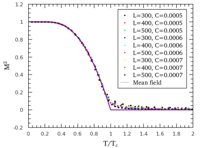
Figure 18: (Color online). Magnetization square vs. temperature over critical temperature computed with Monte Carlo and compared with the mean-field result for various concentrations and sizes.

IV Conclusions

Through extensive DFT calculations we have found that that the interaction between H atoms on graphene favors adsorption on different sublattices along with an antiferromagnetic coupling of the induced magnetic moments. On the contrary, when hydrogenation takes place on the surface of graphite or graphene multilayers (in Bernal stacking), the difference in adsorption energies takes over the interaction between H atoms and may result in all atoms adsorbed on the same sublattice and, thereby, in a ferromagnetic state for low concentrations. Based on the exchange couplings obtained from the DFT calculations, we have also evaluated the Curie temperature by mapping this system onto an Ising-like model with randomly located spins. The long-range nature of the magnetic coupling makes the Curie temperature size dependent and larger than room temperature for typical concentrations and sizes.

V Acknowledgments

This work was supported by MICINN under Grants Nos. FIS2010-21883, CONSOLIDER CSD2007-0010, F1S2009-12721, FIS2012-37549, and by Generalitat Valenciana under Grant PROMETEO/2012/011. We also acknowledge computational support from the CCC of the Universidad Autónoma de Madrid. We thank F. Ynduráin for discussions and I. Brihuega for sharing with us preliminary experimental data.

References

- Gómez-Navarro et al. (2005) C. Gómez-Navarro, P. J. de Pablo, J. Gómez-Herrero, B. Biel, F. J. Garcia-Vidal, a. Rubio, and F. Flores, Nature materials 4, 534 (2005).
- Ugeda et al. (2010) M. M. Ugeda, I. Brihuega, F. Guinea, and J. M. Gómez-Rodríguez, Phys. Rev. Lett. 104, 096804 (2010).
- Jia et al. (2009) X. Jia, M. Hofmann, V. Meunier, B. G. Sumpter, J. Campos-Delgado, J. M. Romo-Herrera, H. Son, Y.-P. Hsieh, A. Reina, J. Kong, et al., Science 323, 1701 (2009).
- Elias et al. (2009) D. C. Elias, R. R. Nair, T. M. G. Mohiuddin, S. V. Morozov, P. Blake, M. P. Halsall, A. C. Ferrari, D. W. Boukhvalov, M. I. Katsnelson, A. K. Geim, et al., Science 323, 610 (2009).
- Sessi et al. (2009) P. Sessi, J. R. Guest, M. Bode, and N. P. Guisinger, Nano letters 9, 4343 (2009).
- Haberer et al. (2010) D. Haberer, D. V. Vyalikh, S. Taioli, B. Dora, M. Farjam, J. Fink, D. Marchenko, T. Pichler, K. Ziegler, S. Simonucci, et al., Nano letters 10, 3360 (2010).
- Yang et al. (2010) M. Yang, A. Nurbawono, C. Zhang, and Y. P. Feng, Applied Physics Letters 96, 193115 (2010).
- Balog et al. (2010) R. Balog, B. Jø rgensen, L. Nilsson, M. Andersen, E. Rienks, M. Bianchi, M. Fanetti, E. Laegsgaard, A. Baraldi, S. Lizzit, et al., Nature materials 9, 315 (2010).
- Soriano et al. (2010) D. Soriano, F. Muñoz-Rojas, J. Fernández-Rossier, and J. J. Palacios, Phys. Rev. B 81, 165409 (2010).
- Zhou et al. (2009) J. Zhou, Q. Wang, Q. Sun, X. S. Chen, Y. Kawazoe, and P. Jena, Nano letters 9, 3867 (2009).
- Sepioni et al. (2010) M. Sepioni, R. R. Nair, S. Rablen, J. Narayanan, F. Tuna, R. Winpenny, A. K. Geim, and I. V. Grigorieva, Phys. Rev. Lett. 105, 207205 (2010).
- Nair et al. (2012) R. R. Nair, M. Sepioni, I.-L. Tsai, O. Lehtinen, J. Keinonen, A. V. Krasheninnikov, T. Thomson, A. K. Geim, and I. V. Grigorieva, Nature Physics 8, 199 (2012).
- McCreary et al. (2012) K. M. McCreary, A. G. Swartz, W. Han, J. Fabian, and R. K. Kawakami, Physical Review Letters 109 186604 (2012).
- Lehtinen et al. (2003) P. O. Lehtinen, A. S. Foster, A. Ayuela, A. Krasheninnikov, K. Nordlund, and R. M. Nieminen, Phys. Rev. Lett. 91, 017202 (2003).
- Boukhvalov et al. (2008) D. W. Boukhvalov, M. I. Katsnelson, and A. I. Lichtenstein, Phys. Rev. B 77, 035427 (2008).
- Casolo et al. (2009) S. Casolo, O. M. Lø vvik, R. Martinazzo, and G. F. Tantardini, The Journal of chemical physics 130, 054704 (2009).
- Soriano et al. (2011) D. Soriano, N. Leconte, P. Ordejón, J.-C. Charlier, J.-J. Palacios, and S. Roche, Phys. Rev. Lett. 107, 016602 (2011).
- Lieb (1989) E. H. Lieb, Phys. Rev. Lett. 62, 1201 (1989).
- Saito et al. (1998) R. Saito, G. Dresselhaus, and S. Dresselhaus, Physical Properties of Carbon Nanotubes (Imperial College Press, 1998).
- Yazyev and Helm (2007) O. V. Yazyev and L. Helm, Phys. Rev. B 75, 125408 (2007).
- Palacios et al. (2008) J. J. Palacios, J. Fernández-Rossier, and L. Brey, Phys. Rev. B 77, 195428 (2008).
- Esquinazi et al. (2003) P. Esquinazi, D. Spemann, R. Höhne, A. Setzer, K. H. Han, and T. Butz, Phys. Rev. Lett. 91, 227201 (2003).
- Ramos et al. (2010) M. A. Ramos, J. Barzola-Quiquia, P. Esquinazi, A. Muñoz-Martin, A. Climent-Font, and M. García-Hernández, Phys. Rev. B 81, 214404 (2010).
- Pauling (1960) L. Pauling, The Nature of the Chemical Bond and the Structure of Molecules and Crystals: An Introduction to Modern Structural Chemistry, George Fisher Baker Non-resident Lectureship in Chemistry at Cornell University (Cornell University Press, 1960).
- Yazyev (2008) O. V. Yazyev, Phys. Rev. Lett. 101, 037203 (2008).
- Hohenberg and Kohn (1964) P. Hohenberg and W. Kohn, Phys. Rev. 136, 864 (1964).
- Kohn and Sham (1965) W. Kohn and L. J. Sham, Phys. Rev. 140, 1133 (1965).
- Ordejón et al. (1996) P. Ordejón, E. Artacho, and J. M. Soler, Phys. Rev. B 53, R10441 (1996).
- Soler et al. (2002) J. M. Soler, E. Artacho, J. D. Gale, A. García, J. Junquera, P. Ordejón, and D. Sánchez-Portal, Journal of Physics: Condensed Matter 14, 2745 (2002).
- Dion et al. (2004) M. Dion, H. Rydberg, E. Schröder, D. C. Langreth, and B. I. Lundqvist, Phys. Rev. Lett. 92, 246401 (2004).
- Román-Pérez and Soler (2009) G. Román-Pérez and J. M. Soler, Phys. Rev. Lett. 103, 096102 (2009).
- Kong et al. (2009) L. Kong, G. Román-Pérez, J. M. Soler, and D. C. Langreth, Phys. Rev. Lett. 103, 096103 (2009).
- Troullier and Martins (1991) N. Troullier and J. L. Martins, Phys. Rev. B 43, 1993 (1991).
- Junquera et al. (2001) J. Junquera, Ó. Paz, D. Sánchez-Portal, and E. Artacho, Phys. Rev. B 64, 235111 (2001).
- Sands (1994) D. E. Sands, Introduction to Crystallography, Dover Classics of Science and Mathematics (Dover Publications, 1994).
- Wallace (1947) P. R. Wallace, Phys. Rev. 71, 622 (1947).
- McClure (1957) J. W. McClure, Phys. Rev. 108, 612 (1957).
- Reich et al. (2002) S. Reich, J. Maultzsch, C. Thomsen, and P. Ordejón, Phys. Rev. B 66, 035412 (2002).
- Latil and Henrard (2006) S. Latil and L. Henrard, Phys. Rev. Lett. 97, 036803 (2006).
- Min et al. (2007) H. Min, B. Sahu, S. K. Banerjee, and A. H. MacDonald, Phys. Rev. B 75, 155115 (2007).
- Tatar and Rabii (1982) R. C. Tatar and S. Rabii, Phys. Rev. B 25, 4126 (1982).
- Ahuja et al. (1997) R. Ahuja, S. Auluck, J. M. Wills, M. Alouani, B. Johansson, and O. Eriksson, Phys. Rev. B 55, 4999 (1997).
- Sha and Jackson (2002) X. Sha and B. Jackson, Surface Science 496, 318 (2002).
- Ivanovskaya et al. (2010) V. V. Ivanovskaya, a. Zobelli, D. Teillet-Billy, N. Rougeau, V. Sidis, and P. R. Briddon, The European Physical Journal B 76, 481 (2010).
- Sljivancanin et al. (2009) Z. Sljivancanin, E. Rauls, L. Hornekaer, W. Xu, F. Besenbacher, and B. Hammer, The Journal of chemical physics 131, 084706 (2009).
- Kerwin and Jackson (2008) J. Kerwin and B. Jackson, The Journal of chemical physics 128, 084702 (2008).
- Denis and Iribarne (2009) P. a. Denis and F. Iribarne, Journal of Molecular Structure: THEOCHEM 907, 93 (2009).
- Duplock et al. (2004) E. J. Duplock, M. Scheffler, and P. J. D. Lindan, Phys. Rev. Lett. 92, 225502 (2004).
- Hornekær et al. (2006) L. Hornekær, E. Rauls, W. Xu, Z. Sljivancanin, R. Otero, I. Stensgaard, E. Lægsgaard, B. Hammer, and F. Besenbacher, Phys. Rev. Lett. 97, 186102 (2006).
- Chen et al. (2007) L. Chen, a. C. Cooper, G. P. Pez, and H. Cheng, Journal of Physical Chemistry C 111, 18995 (2007).
- Palacios and Ynduráin (2012) J. J. Palacios and F. Ynduráin, Phys. Rev. B 85, 245443 (2012).
- (52) E. J. G Santos A. Ayuela, and D. Sánchez-Portal New Journal of Physics 14, 043022 (2012).
- Matsumoto et al. (2001) Y. Matsumoto, M. Murakami, T. Shono, T. Hasegawa, T. Fukumura, M. Kawasaki, P. Ahmet, T. Chikyow, S.-y. Koshihara, and H. Koinuma, Science 291, 854 (2001).
- (54) I. Brihuega, private communication.
- Binder (1981) K. Binder, Zeitschrift fur Physik B Condensed Matter 43, 119 (1981).
- Binder (1981) K. Binder, Phys. Rev. Lett. 47, 693 (1981).
- Binney et al. (1992) J. Binney, J. J. Dowrick, A. T. Fisher, and M. R. S. Newman, The Theory of Critical Phenomena: An Introduction to the Renormalization Group, Oxford Science Publ (Clarendon Press, 1992).
- Heydenreich et al. (2008) M. Heydenreich, R. Hofstad, and A. Sakai, Journal of Statistical Physics 132, 1001 (2008).
- (59) M. Moaied, PhD Thesis. Universidad Autónoma de Madrid, 2014.