Meta-work and the analogous Jarzynski relation in ensembles of dynamical trajectories

Abstract

Recently there has been growing interest in extending the thermodynamic method from static configurations to dynamical trajectories. In this approach, ensembles of trajectories are treated in an analogous manner to ensembles of configurations in equilibrium statistical mechanics: generating functions of dynamical observables are interpreted as partition sums, and the statistical properties of trajectory ensembles are encoded in free-energy functions that can be obtained through large-deviation methods in a suitable large time limit. This establishes what one can call a “thermodynamics of trajectories”. In this paper we go a step further, and make a first connection to fluctuation theorems by generalising them to this dynamical context. We show that an effective “meta-dynamics” in the space of trajectories gives rise to the celebrated Jarzynski relation connecting an appropriately defined “meta-work” with changes in dynamical generating functions. We demonstrate the potential applicability of this result to computer simulations for two open quantum systems, a two-level system and the micromaser. We finally discuss the behavior of the Jarzynski relation across a first-order trajectory phase transition.

1 Introduction

The so-called “thermodynamics of trajectories” approach provides a description of time-ordered dynamic events that is analogous to the thermodynamic description of configurations in space. Using large-deviation methods [1, 2, 3], ensembles of trajectories can be classified by dynamic order parameters and their conjugate fields. This is in effect the thermodynamic formalism of Ruelle [1, 2] applied to the space of trajectories, rather than configurations. Quantities analogous to free-energy densities and entropy densities have been identified, and used to gain insight into rare dynamical behaviours of systems both classical [4, 5, 6, 7, 8, 9, 10, 11, 12, 13, 14, 15, 16] and quantum [17, 18, 19, 20, 21, 22]. Of particular interest has been the identification of dynamical phase transitions into non-equilibrium states with vastly different dynamic properties. To this end, the use of transition path sampling (TPS) [23] has allowed for efficient numerical generation of non-equilibrium states, which has had much success in describing the dynamics of glassy systems [9, 24, 25, 26].

Trajectories and their ensembles also play a central role for the theoretical study of driven non-equilibrium systems that has led to the formulation of a class of relations, called fluctuation theorems [27, 28, 29, 30, 31, 32, 33, 34], which hold arbitrarily far from thermal equilibrium. Of central importance is Jarzynski’s non-equilibrium work relation, which relates the work spent in an arbitrarily fast switching process to the change of free-energy [28, 29]. Given that the thermodynamics of trajectories approach is the generalisation to dynamical ensembles of equilibrium thermodynamics, it is natural to expect that there will also be an analogous extension to trajectory ensembles of the fundamental non-equilibrium relations encoded by the fluctuation theorems. This is the question we address in this work.

The purpose of this paper is two-fold. First, we introduce the concept of processes in the space of trajectories resulting from changing the conjugate field. This allows to identify a meta-work, which, through the analogous Jarzynski relation, allows the computation of the large deviation function. Second, we explore this result in computer simulations of two quantum systems. To this end we employ an algorithm based on transition path sampling while changing the conjugate field. For computational convenience, we work with the recently introduced $x$-ensemble, in which the observation time is the fluctuating order parameter while the number of events is held fixed [35]. Specifically, we study two open quantum systems, the dynamics of which is described by Lindblad master equations [36]. The first system we consider is a dissipative two-level system [37], which can be easily solved analytically and thus provides a simple illustration of our approach. The second model system is the single atom maser, or micromaser [38]. Depending on the parameters, this system exhibits multiple dynamical crossovers, i.e., sharp changes of the mean observation time as we change $x$. It thus allows to investigate the behavior of the Jarzynksi relation as one crosses first-order discontinuities, a situation that seems to have received comparably low attention (see, e.g., Refs. [39, 40] for numerical and Ref. [41] for a mean-field study in the case of the Ising model).

2 Thermodynamic formalism and ensembles of trajectories

The probability distribution of some observable $E$, under rather mild conditions, gives rise to a formal structure that is known from thermodynamics. The first condition is that $E$ is extensive, i.e., there is a “system size” $K$ and the mean of $e=E/K$ remains both nonzero and finite as $K\rightarrow\infty$. Second, the probability of $E$ takes on a large deviation form, $P(E)\asymp e^{-K\phi(e)}$, with $\phi(e)$ independent of $K$. For example, in equilibrium statistical physics, if $K$ is the number of particles in a closed volume and $E$ the energy, the function $\phi(e)$ is immediately identified as the negative specific entropy. In this case, the partition sum

$$Z(\beta)=\int\rmd E\;P(E)e^{-\beta E}\asymp e^{Kg(\beta)}$$ (1)

also has a large deviation form involving the free-energy per particle $g(\beta)$, see Ref. [3] for a general introduction. Both entropy and free-energy are related by a Legendre transform,

$$g(\beta)=-\min_{e}[\phi(e)+\beta e],$$ (2)

which describes the transformation between the micro-canonical ensemble at fixed $e$ to the canonical ensemble at fixed inverse temperature $\beta$.

This thermodynamic formalism can be extended to dynamic processes, where now $K$ denotes the the observation time. In this case the mathematical structure remains the same but one of course loses the immediate physical interpretation of the canonical ensemble. Here we consider systems evolving in time due to their physical, stochastic dynamics. Hence, over a given time $t_{\mathrm{obs}}$ we can define trajectories

$$\chi\equiv\{z_{t}|0\leqslant t\leqslant t_{\mathrm{obs}}\}$$ (3)

recording the random sequence of microstates $z$ the system has visited. We characterize trajectories by an order parameter that plays the role extensive quantities, such as energy, play in conventional thermodynamics. Examples for these dynamical order parameters include the total number of transitions (or “jumps”) [42] in a trajectory, the total number of certain specific events, the time-integral of the mobility of particles [9, 25], or the time-integral of the number of particles that are part of a specific structure [26]. For clarity of presentation, we consider a single order parameter but the extension to more than one is straightforward. The crucial property of admissible order parameters is that they are extensive in space and time.

The parameter $K$, which determines the size of trajectories and the corresponding large-size limit, can be something other than the total observation time [43, 35]. In keeping with our thermodynamic analogy, this would correspond to two distinct trajectory ensembles. For definiteness, we will work here specifically with the recently introduced $x$-ensemble [35] although our results are valid more generally. Consider a system in which it is possible to identify and count some event, the specific nature of the event is unimportant, and could be, for example, photon emissions from an atomic system. These events are separated by waiting times $t_{n}$. We define the probability that observing $K$ events takes a particular amount of time, $t_{\mathrm{obs}}\equiv\sum_{n=1}^{K}t_{n}$, which in the large-$K$ limit takes on a large deviation form

$$P_{K}(t_{\mathrm{obs}})\equiv\int\mathcal{D}\chi\;\rho_{0}(\chi)\delta(t_{\mathrm{obs}}(\chi)-t_{\mathrm{obs}})\asymp e^{-K\phi(\tau)},$$ (4)

where $\rho_{0}(\chi)$ denotes the probability distribution of trajectories, as given by the dynamics under consideration, $\tau\equiv t_{\mathrm{obs}}/K$ is the average waiting time within a single trajectory, and the rate function $\phi(\tau)$ quantifies how fluctuations of $\tau$ decay as the number of events is increased. The functional measure $\mathcal{D}\chi$ of paths implies normalization, $\int\mathcal{D}\chi\;\rho_{0}(\chi)=1$.

Taking the Laplace transform of the probability Eq. (4) defines the moment generating function

$$Z_{K}(x)\equiv\int_{0}^{\infty}\rmd t_{\mathrm{obs}}\;P_{K}(t_{\mathrm{obs}})e^{-xt_{\mathrm{obs}}}\asymp e^{Kg(x)}.$$ (5)

Its logarithm defines the cumulant generating function (CGF) $g(x,K)\equiv\ln Z_{K}(x)/K$, which also has a large-deviation form in the limit of which $g(x)$ becomes independent of $K$. In analogy with thermodynamics, $\phi(\tau)$ and $g(x)$ are identified as the associated (negative) entropy density and free-energy density, respectively, which are related through the Legendre transform Eq. (2). Pursuing the analogy with thermodynamics further through identifying the number of events $K$ with particle numbers and the trajectory length $t_{\mathrm{obs}}$ with a volume, $x$ is analogous to the field conjugate to volume with fixed particle numbers, i.e., a pressure. We have thus introduced a “canonical” ensemble of trajectories [44]

$$\rho_{x}(\chi)\equiv\frac{\rho_{0}(\chi)e^{-xt_{\mathrm{obs}}(\chi)}}{Z_{K}(x)}$$ (6)

where $\rho_{x}(\chi)$ is the probability of a trajectory $\chi$ at fixed $x$ (rather than fixed $K$). Physical dynamics takes place at $x=0$, while $x\neq 0$ probes the statistics of atypical trajectories. For details see [35].

3 Jarzynski relation in trajectory space

3.1 Meta-dynamics: Dynamics in the space of trajectories

The situation considered by the Jarzynski relation is that of a system initially in thermal equilibrium with a heat reservoir, where the system is subsequently driven away from equilibrium by externally changing one or more parameters. The dynamics of the system obeys detailed balance with respect to the stationary distribution corresponding to the instantaneous values of the control parameters. Non-equilibrium can then be described as a “lag” between this stationary distribution and the actual distribution [45]. The Jarzynski relation [28] relates the average over all trajectories with the change of free-energy between initial and final state.

In the trajectory ensemble, we are interested in a very similar situation, where we want to determine the function $g(x)$ over a range of values $x$. Instead of performing many “equilibrated” simulation runs at fixed $x$, we aim to extract the function $g(x)$ while changing $x$. To this end we require to notion of a meta-dynamics and a meta-time, which for convenience we take as integer, enumerating the sequence of generated trajectories $\vec{\chi}\equiv(\chi_{0},\dots,\chi_{N})$. The meta-dynamics that generates these trajectories is required to obey detailed balance with respect to the distribution $\rho_{x}(\chi)$, that is,

$$\rho_{x}(\chi)p_{x}(\chi\rightarrow\chi^{\prime})=\rho_{x}(\chi^{\prime})p_{x}(\chi^{\prime}\rightarrow\chi),$$ (7)

where $p_{x}(\chi\rightarrow\chi^{\prime})$ is the probability to generate the trajectory $\chi$ given a previous trajectory $\chi^{\prime}$, and $\rho_{x}(\chi)$ is defined in Eq. (6). Natural candidates for the algorithm used to generate new trajectories are based on transition path sampling and the specific algorithm used in this work is that of [35] (also detailed for completeness in A).

3.2 Meta-work and the Jarzynski relation

Equation (6) has the form of an equilibrium Boltzmann distribution, where $E_{x}(\chi)=xt_{\mathrm{obs}}(\chi)$ can be identified as the analog of an “energy”. Suppose that we change $x$ along the sequence $\vec{\chi}$: We start with a value $x_{0}$ for the biasing field and generate the initial trajectory $\chi_{0}$. We then change the value of $x_{0}$ to $x_{1}$ and generate the next trajectory $\chi_{1}$ of the sequence and so on. The change of the “energy” along the whole sequence is

$$\Delta E\equiv E_{x_{N}}(\chi_{N})-E_{x_{0}}(\chi_{0})=W+Q,$$ (8)

which can be split into two sums

$$Q\equiv\sum_{i=0}^{N-1}[E_{x_{i+1}}(\chi_{i+1})-E_{x_{i+1}}(\chi_{i})],\quad W\equiv\sum_{i=0}^{N-1}[E_{x_{i+1}}(\chi_{i})-E_{x_{i}}(\chi_{i})].$$ (9)

These sums are identified as “heat” $Q$ and “work” $W$, respectively. In particular, the meta-work

$$W=\sum_{i=0}^{N-1}(x_{i+1}-x_{i})t_{\mathrm{obs}}(\chi_{i})$$ (10)

sums the incremental changes of the “energy” due to a change of the field $x$ for the same trajectory.

We can now prove the Jarzynski relation following standard arguments by combining the form of the path probability Eq. (6) with Eq. (7). Consider the average

$$\langle e^{-W}\rangle=\int\mathcal{D}\chi_{0}\cdots\mathcal{D}\chi_{N}\;\rho_{x_{0}}(\chi_{0})p_{x_{1}}(\chi_{0}\rightarrow\chi_{1})\cdots p_{x_{N}}(\chi_{N-1}\rightarrow\chi_{N})e^{-W}$$ (11)

The first integral reads

$$\frac{1}{Z(x_{0})}\int\mathcal{D}\chi_{0}\;\rho_{0}(\chi_{0})p_{x_{1}}(\chi_{0}\rightarrow\chi_{1})e^{-x_{1}t_{\mathrm{obs}}(\chi_{0})}$$ (12)

$$=\frac{Z_{K}(x_{1})}{Z_{K}(x_{0})}\int\mathcal{D}\chi_{0}\;\rho_{x_{1}}(\chi_{0})p_{x_{1}}(\chi_{0}\rightarrow\chi_{1})=\frac{Z_{K}(x_{1})}{Z_{K}(x_{0})}\rho_{x_{1}}(\chi_{1}).$$

Unraveling all terms thus leads to

$$\langle e^{-W}\rangle=\frac{Z_{K}(x_{N})}{Z_{K}(x_{0})},$$ (13)

which is the analogous Jarzynski relation for the meta-work in canonical ensembles of trajectories.

3.3 Computing the meta-free-energy $g(x)$

From Eq. (13), we can extract the change of the trajectory (or meta-) free-energy

$$\Delta g\equiv g(x_{N})-g(x_{0})=\lim_{K\rightarrow\infty}\frac{1}{K}\ln\langle e^{-W}\rangle$$ (14)

from the meta-work. Using this result, the free-energy $g(x)$ of the $x$-ensemble can be calculated from simulation in the following way. A trajectory with fixed number of events $K$ is created and equilibrated to the desired starting value $x_{0}$ using the $x$-ensemble TPS algorithm described in appendix A. This is basically a Monte Carlo algorithm accepting or rejecting proposed trajectories employing the Metropolis criterion. The system then moves along the “forward” path up to the desired maximum value $x_{N}$ in a series of steps. For simplicity, we consider a linear protocol $x_{i}=x_{0}+i(x_{N}-x_{0})/N$ although other protocols might be more suitable. Each step corresponds to a single change to the trajectory whether the proposed change is accepted under the Metropolis criterion or not.

This process is repeated $M$ times until a good distribution of meta-work for both the forward and the reverse process (going from $x_{N}$ to $x_{0}$) is built up. The free-energy difference between $x_{N}$ and $x_{0}$ can then be computed with an iterative Bennett’s Acceptance Ratio (BAR) method [46, 47],

$$\Delta g^{(k+1)}=-\ln\frac{\sum_{j=1}^{M}\left[1+e^{W_{\uparrow,j}-\Delta g^{(k)}}\right]^{-1}}{\sum_{j=1}^{M}\left[e^{W_{\downarrow,j}}+e^{-\Delta g^{(k)}}\right]^{-1}},$$ (15)

where the sum over $j$ denotes the sum over the work values for each repetition of forward ($\uparrow$) and reverse ($\downarrow$) process. The work values are random numbers with probability distributions $P_{\uparrow}(W)$ and $P_{\downarrow}(W)$, respectively.

As is the case in thermodynamic problems, there need be some overlap in the work distributions for the forward and reverse processes, but the rate at which these processes occur need not be slow enough to ensure equilibrium at all points (resulting in completely overlapping work distributions). Strictly speaking, the large-deviation function $g(x)$ is defined in the limit of $K\to\infty$. In practice, for the numerical estimation of $g(x)$, the length of individual trajectories as defined by the number of events $K$ is not critical to the result, provided the meta free-energies are scaled per event. Furthermore, while short trajectories of low $K$ necessarily require less computation time, they also necessarily have much larger fluctuations in work distributions, requiring more repetitions to build a reasonable distribution numerically, meaning there is some trade off in efficiency. Note however that a positive aspect of these fluctuations is that the broadening of work distributions can lead to an increase in their overlap. These considerations indicate that the optimal trajectory length, and number of steps to calculate the effective meta free-energies as efficiently as possible, are highly system dependent.

4 Application to open quantum systems

For the purpose of demonstrating the validity of the analogous Jarzynski equality (13), we consider simple open quantum systems whose dynamics are described by Lindblad master equations of the form

$$\frac{d}{dt}\rho=-i[H,\rho]+\sum_{\alpha=1}^{N_{L}}\big{(}L_{\alpha}\rho L_{\alpha}^{\dagger}-\frac{1}{2}\{L_{\alpha}^{\dagger}L_{\alpha},\rho\}\big{)},$$ (16)

where $N_{L}$ is the number of dissipative terms and the $L_{\alpha}$ are the corresponding jump operators [48, 37, 36]. Throughout, $\hbar$ is set to unity. The countable events are associated with action under the Lindblad operators (usually photon emission/absorption). Such systems are well suited to simulation using continuous-time Monte Carlo algorithms [37].

4.1 2-Level System

We consider a laser-driven two-level system, which exchanges photons with a radiation bath [37]. The system is comprised of levels $\left|0\right\rangle$ and $\left|1\right\rangle$ with Hamiltonian

$$H=\Omega(\sigma+\sigma^{\dagger})$$ (17)

and two jump operators

$$L_{1}=\sqrt{\kappa}\sigma,\qquad L_{2}=\sqrt{\gamma}\sigma^{\dagger}$$ (18)

corresponding to photon emission and absorption, respectively. Here $\sigma=\left|0\right\rangle\left\langle 1\right|$ and $\sigma^{\dagger}=\left|1\right\rangle\left\langle 0\right|$ are lowering and raising operators, and $\Omega$ is the Rabi frequency of the driving laser. As such, the system emits photons and is projected onto $\left|0\right\rangle$ with rate $\kappa$, and absorbs photons and is projected into $\left|1\right\rangle$ state with rate $\gamma$. The counted events $K$ are any photon emission or absorption, i.e., the total number of quantum jumps.

We consider first the zero-temperature case ($\gamma=0$), for which there is only one jump - described by action under $L_{1}$ (photon emission). The large deviation function in this case reads

$$g(x)=-3\ln{\left(1+\frac{x}{2}\right)}$$ (19)

This result is obtained by inverting $g(x)=\theta^{-1}(x)$, where $\theta(s)$ is the largest eigenvalue of the deformed master equation associated with the $s$-ensemble, see Ref. [35] for details.

Figure  1 provides a numerical test of the Jarzynski relation (13) for trajectories with $K=20$ events. We have sampled $M=5000$ trajectories for the forward and backward protocol, where trajectories started from an initial $x_{0}=0$ (equilibrium) state to a final state ranging between $x=-1$ and $x=1.5$, with $N=1000$ TPS step moves for each direction. As criterion to stop the BAR iterations, we chose the threshold $10^{-5}$ for the fractional change of the estimated $g(x)$ between iterations. For this system convergence is reached very fast taking typically 2-3 iterations, and there is a good agreement between the results obtained from the Jarzynski relation and the exact results.

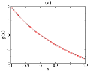
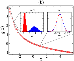
Figure 1: 2-level system. (a) Comparison of the meta-free-energy $g(x)$ obtained numerically via the trajectory Jarzynski relation (symbols) to the exact analytical result (19) (solid line) for a range of $x$, in the zero temperature case, with $\kappa=4\Omega$. (b) Same as in (a), but now for the finite temperature case, with $\kappa=6\Omega$ and $\gamma=2\Omega$. The statistical error is smaller than the symbol sizes. Insets to (b): Sampled histograms for the meta-work distribution $P_{\uparrow}(W)$ for the forward (red) and $P_{\downarrow}(-W)$ for the backward process (blue), at the two final values of $x$ shown.

We now consider the finite temperature case with parameters $\kappa=6\Omega$, $\gamma=2\Omega$. Here action under both $L_{1}$ and $L_{2}$ occurs, and so there are two jump possibilities. Fig. 1(b) provides a numerical test of the Jarzynski relation in this case. Analytical results are again obtained from the largest eigenvalue of the deformed master operator corresponding to the $s$-ensemble, and inverted to give the $x$-ensemble meta-free-energy $g(x)$. The exact expression is available but cumbersome and rather unilluminating to be given explicitly. Note that the true $g(x)$ diverges close to $x\simeq-3.5$ [cf. with the zero temperature case, Eq. (19), where the limiting value is $x=-2$]. Again, $M=5000$ iterations were used for trajectories of $K=20$ events but with now $N=5\times 10^{5}$ TPS step moves for each iteration. While there is a good agreement between the results obtained from the Jarzynski relation and the exact results for a broad range of $x_{N}$, we have extended the plotted range of $x$ values to demonstrate that the numerical estimate for $g(x)$ starts to divert from its analytical prediction as we approach the divergence. For $x<0$ the “pressure” is negative, selecting rare trajectories with large trajectory length $t_{\mathrm{obs}}$. Our numerical procedure breaks down because it takes an increasing amount of time to equilibrate the system at the final $x$ for the backward iterations. For the forward-backward protocol, $N$ has to be sufficiently large to generate work distributions that sufficiently overlap in order for Eq. (15) to work. This is demonstrated in the inset of Fig. 1(b). This is a general feature of the Jarzynski relation. Although in principle it holds for any driving speed and any protocol, application to data requires either to sample extreme work values sufficiently or to generate distributions from forward and backward protocols that overlap.

4.2 Micromaser

The micromaser provides a useful test of a pseudo-many-body system, as well as a system with many first-order phase transitions in the $x$-ensemble. A detailed account of the model can be found in Ref. [38] and is only briefly summarized here. A cavity is pumped by excited two-level atoms and it also interacts with a thermal bath. The system is described by a single bosonic mode evolving according to a Lindblad master equation with four Lindblad terms, two corresponding to the cavity-atom interactions,

$$L_{1}=\sqrt{r}\frac{\sin(\phi\sqrt{aa^{\dagger}})}{\sqrt{aa^{\dagger}}},\qquad L_{2}=\sqrt{r}\cos(\phi\sqrt{aa^{\dagger}}),$$ (20)

and two corresponding to the cavity exchanging photons with a radiation bath,

$$L_{3}=\sqrt{\kappa},\qquad L_{4}=\sqrt{\gamma}a^{\dagger}.$$ (21)

Here, $a$ and $a^{\dagger}$ are the raising and lowering operators of the cavity mode, respectively, and $\kappa$ and $\gamma$ are the rates of photon emission and absorption to/from the radiation bath. The parameter $\varphi$ encodes the information on the atom-cavity interaction and $r$ is the atom beam rate through the cavity. The system can be parametrised by a single “pump parameter” $\alpha\equiv\varphi\sqrt{r/(\kappa-\gamma)}$. The events being counted are the actions under any of the four Lindblad terms.

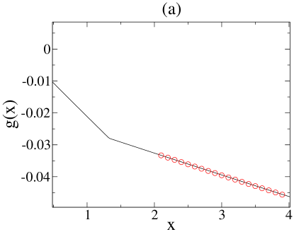
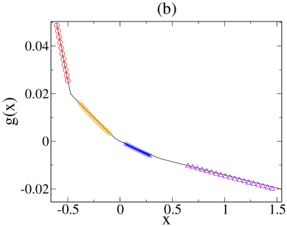
Figure 2: Micromaser. (a) Comparison of the meta-free-energy $g(x)$ obtained numerically via the trajectory Jarzynski relation (symbols) to results obtained by direct diagonalisation of the master operator (solid line) for $\alpha=1.2\pi$, where the system is initially equilibrated to $x=2$. (b) Same as in (a), but now for $\alpha=4\pi$. Different simulations, equilibrated to different initial values of $x$ are denoted by different symbols.

Despite being a system with a single degree of freedom, the micromaser has a rich dynamical behaviour due to the combination of an infinite dimensional Hilbert space and the non-linear jump operators $L_{1}$ and $L_{2}$. In particular, it displays a number of distinct dynamical phases and transitions between them [49, 50, 51]. (Strictly speaking, these are sharp crossovers which only become singular in the limit of $r\to\infty$; see [52, 50].) Note also that in the dynamics generated by the operators (20-21) an initial density matrix that is diagonal stays diagonal for all times. Due to this, the dynamics of the micromaser, while quantum in origin, is in effect that of a classical stochastic system.

We first attempt to compute meta-free-energy differences within a single phase. Fig. 2(a) provides a numerical test of the Jarzynski relation for a pump parameter of $\alpha=1.2\pi$. The trajectories are initially equilibrated to a non-equilibrium dynamical phase with $x_{0}=2$, and the Jarzynski protocol run for trajectories of $K=1000$ jumps, with $M=5000$ iterations and $N=60000$ TPS step moves per iteration. The computed meta-free-energy differences are compared to results obtained from direct diagonalisation of the master operator, as in [49], and a good agreement is found between the two methods. Provided the existence of phases, and the boundaries between them, is known, a complete picture of meta free-energy differences can be constructed even when there are multiple dynamical phases. For example, with the pump parameter taking a value of $\alpha=4\pi$, four distinct phases occur [49, 50], see Fig. 2(b), and $g(x)$ can be computed within phases by initially equilibrating the trajectories to a value of $x$ within the required phase. Again trajectories of $K=1000$ jumps were used, with $M=5000$ iterations and $N=60000$ TPS step moves per iteration.

4.3 Driving across a first-order phase transition

We finally examine the behavior of the Jarzynski relation using a protocol $x_{0}\rightarrow x_{N}$ that crosses a phase boundary $x^{\ast}$ at a finite speed. In the quasi-stationary limit of $N\rightarrow\infty$, we obtain from the definition Eq. (5) the well-known expression

$$\ln\frac{Z_{K}(x_{N})}{Z_{K}(x_{0})}=\int_{x_{0}}^{x_{N}}\rmd x\;\frac{\partial\ln Z_{K}(x)}{\partial x}=-\int_{x_{0}}^{x_{N}}\rmd x\;\langle t_{\mathrm{obs}}\rangle_{x}$$ (22)

for thermodynamic integration, where the subscript emphasizes that the average is calculated from equilibrated trajectories at fixed $x$. Eq. (22) is known to fail in the presence of a discontinuous phase transition, not because the equation is wrong but because of the way a simulation is carried out in practice. Typically, one will apply a small change $x_{i}\rightarrow x_{i+1}$, let the system relax, and then record data to calculate the average. Crossing $x^{\ast}$, the system will not immediately adapt to the new state but follow the metastable branch due to the cost of nucleating the new stable phase, thus violating the assumption that the calculated mean corresponds to the true equilibrium mean. In the micromaser, sharp crossovers occur at certain values of the biasing field between phases that can be characterised by either their average emission rate, or the closely related expected photon occupation of the cavity [49, 50, 51]. When considering these transitions in the context of the $x$-ensemble, different phases have significantly different average trajectory lengths for the same fixed number of quantum jumps [35]. Just like in ordinary first-order transitions, pronounced metastability may prevent from estimating meta free-energies accurately with (22). This can occur when the transition at $x^{\ast}$ is between phases with very different activities. In this case, if trajectories are prepared in the less active phase (for example starting from $x=0$ and increasing $x$), the barrier to nucleate the more active phase when $x>x^{\ast}$ can be prohibitive for practical simulation. The nucleation event can be promoted externally, for example by altering the photon occupation of the cavity by temporarily increasing the pump parameter (or similar “parallel tempering”). But without such external interference the timescale for nucleating the new stable phase is often beyond what can be reasonably simulated.

One could hope that the Jarzynski relation, given that it applies to arbitrarily fast non-equilibrium protocols, would provide a way out of this problem since trajectories can be sampled at finite rate for the change in $x$. In practice, however, even with slow driving speeds it is problematic to compute free-energy differences across first-order phase boundaries. Results for the micromaser are shown in Fig. 3 (for a pump parameter of $\alpha=1.2\pi$ and with $\frac{\gamma}{\kappa}=0.15$ corresponding to a temperature $T=0.5$ [49, 35]). Trajectories with $K=2000$ jumps were sampled for $M=5000$ iterations, with $N=10^{6}$ TPS step moves for each iteration. For the chosen parameters, the system is known to undergo a first-order transition at $x^{\ast}\simeq 1.34$ [35]. The computed free-energy difference using the Jarzinsky relation gets locked to the phase that is stable for $x<x^{\ast}$ but which becomes metastable for $x>x^{\ast}$. This is evident by the fact that the computed free-energy follows the path of the eigenvalue that dominates for $x<x^{\ast}$, but which becomes subdominant at $x>x^{\ast}$.

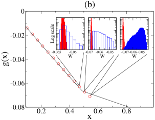
Figure 3: Micromaser with cross-phase Jarzynski protocol. (a) Comparison of the numerical meta free-energy, $g(x)$, obtained numerically via the Jarzynski relation (symbols) to results obtained by direct diagonalisation (solid line) in a micromaser with pump parameter $\alpha=1.2\pi$, at a finite temperature (${\gamma}/{\kappa}=0.15$). The second largest eigenvalue (dashed line) is plotted to illustrate the meta free-energy calculation being locked to the metastable branch after the transition. Inset to (a): the expected waiting time per event showing the differing dynamic properties of the two phases. (b) Same as in (a), but now at zero temperature (${\gamma}/{\kappa}=0$). Insets to (b): sampled meta-work distributions for the forward (red) and backward (blue) process for the three points shown.

This locking in the metastable branch occurs even if one reduces the difference in the dynamic properties between the two phases, for example by considering zero temperature and for smaller beam rate [49], or improves the sampling (for example by doubling the number of interations), see Fig. 3(b). The cause can be understood by looking at the meta-work distributions for the forward and reverse processes, see insets to Fig. 3(b). For the conditions shown, the driving is slow enough for the forward and reverse meta-work distributions to overlap immediately before the phase transition. However as the phase boundary is crossed the two become separated. A small residual spike of the reverse distribution lies within the bulk of the forward distribution, corresponding to a small fraction of cases where the reverse process starts in the metastable phase. This occurs precisely because the simulation cannot be done in the “thermodynamic limit” of $K\rightarrow\infty$ and $r/(\kappa-\gamma)\rightarrow\infty$, i.e.  the transition is not strictly a phase transition but a very sharp crossover [50]. Thus when differences in the meta free-energy $g(x)$ is computed with the BAR method, it only sees the metastable phase. It is worth noting that these attempts to compute a cross-phase free-energy difference took two orders of magnitude more computation than any of the single-phase free-energy computations.

5 Concluding remarks

We have extended the “thermodynamics of trajectories” method to show the existence of analogous fluctuation theorems associated with corresponding “non-equilibrium” processes. In particular, we have studied the analogous Jarzynski relation connecting meta-work to changes in trajectory free-energies. For convenience, we have considered ensembles of trajectories characterised by a fixed number of configuration changes (or jumps) and variable overall time [35]. The parameter that was driven was the field conjugate to the total trajectory time, and the meta-time associated to this non-equilibrium procedure was that of the TPS scheme used to evolve trajectories in trajectory space. The associated work, or meta-work, was given by the path integral of the change in average total trajectory time, i.e., the change in the trajectory observable conjugate to the driven field, again in analogy with what occurs with configuration ensembles. The analogous Jarzynski relation connects the average of the exponential of this meta-work over the driven process to the difference of the large-deviation rate functions that determine the trajectory ensembles at the endpoint values of the driven field. Similar relations hold in other trajectory ensembles, for example that of trajectories of fixed total time and where the number of events fluctuates.

Our results here further underpin the thermodynamics approach to dynamics. Not only ensembles of dynamical trajectories can be studied by generalising equilibrium statistical mechanics via large deviation methods, but also non-equilibrium statistical mechanics tools can be generalised and applied to uncover properties of such ensembles. By considering the analogous Jarzynski relation we have shown that the large-deviation function that encodes the properties of one trajectory ensemble can be obtained by considering the statistics of the meta-work performed as the parameter that characterises the ensemble is driven.

A further interesting observation is the following. The general relation between forward and backward processes that underpins most integral fluctuation theorems is a straightforward consequence of probability conservation [34]. Few integral fluctuation relations are “non-trivial” in the sense of conveying actually useful information about the problem studied. This occurs when one can write the stationary distribution in terms of “weights” that encode their functional dependence on the objects that form the ensemble under consideration (usually configurations; trajectories in our case), and a “free-energy”. For ensembles of configurations, these include the Jarzynski relation proper [28, 29] and the Hatano-Sasa relation [32] for driven stationary states. We note that the class of trajectory ensemble problems we studied here adds to this small group. These are cases where the “normalisation constant” of the stationary probability distribution also has physical meaning, as it is given by the large-deviation function which is the generating function for moments and cumulants of time-integrated and thus play the role of trajectory free-energies.

Appendix A Sampling algorithm

For completeness, here we describe the algorithm used to sample trajectories. This algorithm is an adaptation of the Crooks-Chandler method [53] described in section 3.4 of Ref. [23]; see also [43, 35].

1. Fix total event numbers $K$

2. Generate and store a random number/set of random numbers, $\{r\}_{i}$ as needed to describe each event, defining a complete trajectory, $\chi$.

3. Calculate the total time taken by the trajectory, $t_{\mathrm{obs}}$.

4. Set $x$ to 0.

5. Randomly select and modify a single random number set, $\{r\}_{i}\to\{r^{\prime}\}_{i}$ to propose a new trajectory, $\chi^{\prime}$

6. Recalculate the event $\{r\}_{i}$, and any subsequent events that are altered by the modified result of event $i$. If at any point the state of trajectory $\chi^{\prime}$ is identical to that of $\chi$ after jump $i+\Delta i$ further computation of the trajectory is unnecessary.

7. Calculate the new trajectory length, $t_{\mathrm{obs}}^{\prime}$

8. Accept/Reject the new trajectory based on the metropolis acceptance critera $P_{\mathrm{accept}}=\min\{1,e^{-x(t_{\mathrm{obs}}^{\prime}-t_{\mathrm{obs}})}\}$

9. Repeat steps (v)-(viii) until the trajectory is equilibrated to the current values of $x$

10. Increment $x$ by some small $\delta x$

11. Repeat steps (v)-(xi) until the desired final value of $x$ is reached

References

References

- [1] J. P. Eckmann and D. Ruelle, Rev. Mod. Phys. 57, 617 (1985).
- [2] D. Ruelle, Thermodynamic formalism (Cambridge University Press, 2004).
- [3] H. Touchette, Phys. Rep. 478, 1 (2009).
- [4] J. L. Lebowitz and H. Spohn, J. Stat. Phys. 95, 333 (1999).
- [5] M. Merolle, J. P. Garrahan and D. Chandler, Proc. Natl. Acad. Sci. U.S.A. 102, 10837 (2005).
- [6] V. Lecomte and J. Tailleur, J. Stat. Mech. P03004 (2007).
- [7] J. P. Garrahan, R. L. Jack, V. Lecomte, E. Pitard, K. van Duijvendijk and F. van Wijland, Phys. Rev. Lett. 98, 195702 (2007).
- [8] A. Baule and R. M. L. Evans, Phys. Rev. Lett. 101, 240601 (2008).
- [9] L. O. Hedges, R. L. Jack, J. P. Garrahan and D. Chandler, Science 323, 1309 (2009).
- [10] R. L. Jack and J. P. Garrahan, Phys. Rev. E 81, 011111 (2010).
- [11] C. Giardina, J. Kurchan, V. Lecomte and J. Tailleur, J. Stat. Phys. 145, 787 (2011).
- [12] E. Pitard, V. Lecomte and F. V. Wijland, Europhys. Lett. 96, 56002 (2011).
- [13] C. Flindt and J. P. Garrahan, Phys. Rev. Lett. 110, 050601 (2013).
- [14] R. Chetrite and H. Touchette, Phys. Rev. Lett. 111, 120601 (2013).
- [15] V. Chikkadi, D. Miedema, B. Nienhuis and P. Schall, arXiv:1401.2100 .
- [16] T. Nemoto and S. Sasa, Phys. Rev. Lett. 112, 090602 (2014).
- [17] M. Esposito, U. Harbola and S. Mukamel, Rev. Mod. Phys. 81, 1665 (2009).
- [18] J. P. Garrahan and I. Lesanovsky, Phys. Rev. Lett. 104, 160601 (2010).
- [19] A. A. Budini, Phys. Rev. E 84, 061118 (2011).
- [20] J. Li, Y. Liu, J. Ping, S.-S. Li, X.-Q. Li and Y. Yan, Phys. Rev. B 84, 115319 (2011).
- [21] D. A. Ivanov and A. G. Abanov, Phys. Rev. E 87, 022114 (2013).
- [22] A. Gambassi and A. Silva, Phys. Rev. Lett. 109, 250602 (2012).
- [23] C. Dellago, P. G. Bolhuis and P. L. Geissler, Adv. Chem. Phys. 123, 1 (2002).
- [24] Y. S. Elmatad and A. S. Keys, Phys. Rev. E 85, 061502 (2012).
- [25] T. Speck and D. Chandler, J. Chem. Phys. 136, 184509 (2012).
- [26] T. Speck, A. Malins and C. P. Royall, Phys. Rev. Lett. 109, 195703 (2012).
- [27] G. Gallavotti and E. G. D. Cohen, Phys. Rev. Lett. 74, 2694 (1995).
- [28] C. Jarzynski, Phys. Rev. Lett. 78, 2690 (1997).
- [29] C. Jarzynski, Phys. Rev. E 56, 5018 (1997).
- [30] J. Kurchan, J. Phys. A 31, 3719 (1998).
- [31] G. E. Crooks, Phys. Rev. E 60, 2721 (1999).
- [32] T. Hatano and S. Sasa, Phys. Rev. Lett. 86, 3463 (2001).
- [33] C. Bustamante, J. Liphardt and F. Ritort, Physics Today 43 (2005).
- [34] U. Seifert, Rep. Prog. Phys. 75, 126001 (2012).
- [35] A. A. Budini, R. M. Turner and J. P. Garrahan, J. Stat. Mech. P03012 (2014).
- [36] C. W. Gardiner and P. Zoller, Quantum Noise (Springer, 2004).
- [37] M. B. Plenio and P. L. Knight, Rev. Mod. Phys. 70, 101 (1998).
- [38] B.-G. Englert, arXiv:quant-ph/0203052 (2002).
- [39] C. Chatelain and D. Karevski, J. Stat. Mech. P06005 (2006).
- [40] A. K. Hartmann, Phys. Rev. E 89, 052103 (2014).
- [41] A. Imparato and L. Peliti, Europhys. Lett. 70, 740 (2005).
- [42] J. P. Garrahan, R. L. Jack, V. Lecomte, E. Pitard, K. van Duijvendijk and F. van Wijland, J. Phys. A 42, 075007 (2009).
- [43] P. G. Bolhuis, J. Chem. Phys. 129, 114108 (2008).
- [44] R. Chetrite and H. Touchette, Phys. Rev. Lett. 111, 120601 (2013).
- [45] S. Vaikuntanathan and C. Jarzynski, EPL 87, 60005 (2009).
- [46] C. H. Bennett, J. Comp. Phys. 22, 245 (1976).
- [47] M. R. Shirts, E. Bair, G. Hooker and V. S. Pande, Phys. Rev. Lett. 91, 140601 (2003).
- [48] G. Lindblad, Comm. Math. Phys 48, 119 (1976).
- [49] J. P. Garrahan, A. D. Armour and I. Lesanovsky, Phys. Rev. E 84, 021115 (2011).
- [50] M. van Horssen and M. Guta, arXiv:1206.4956 .
- [51] I. Lesanovsky, M. van Horssen, M. Guta and J. P. Garrahan, Phys. Rev. Lett. 110, 150401 (2013).
- [52] C. Catana, M. van Horssen and M. Guta, Phil. Trans. Royal Soc. A 370, 5308 (2012).
- [53] G. E. Crooks and D. Chandler, Phys. Rev. E 64, 026109 (2001).