Excited state TBA and renormalized TCSA in the scaling Potts model

Abstract

We consider the field theory describing the scaling limit of the Potts quantum spin chain using a combination of two approaches. The first is the renormalized truncated conformal space approach (TCSA), while the second one is a new thermodynamic Bethe Ansatz (TBA) system for the excited state spectrum in finite volume. For the TCSA we investigate and clarify several aspects of the renormalization procedure and counter term construction. The TBA system is first verified by comparing its ultraviolet limit to conformal field theory and the infrared limit to exact S-matrix predictions. We then show that the TBA and the renormalized TCSA match each other to a very high precision for a large range of the volume parameter, providing both a further verification of the TBA system and a demonstration of the efficiency of the TCSA renormalization procedure. We also discuss the lessons learned from our results concerning recent developments regarding the low-energy scattering of quasi-particles in the quantum Potts spin chain.

1 Introduction

In this work we consider the field theory describing the vicinity of the critical point of the three-state Potts quantum spin chain. The model is defined on the Hilbert space

$$\mathcal{H}_{\mathrm{chain}}=\bigotimes_{i}\left(\mathbb{C}^{3}\right)_{i}$$ (1.1)

where $i$ labels the sites of the chain, and the quantum space $\mathbb{C}^{3}$ at site $i$ has the basis $|\alpha\rangle$, $\alpha=0,1,2$, corresponding to the spin degrees of freedom. The dynamics is defined by the Hamiltonian invariant under $\mathbb{S}_{3}$ permutation symmetry

$$H_{\mathrm{chain}}=-J\sum_{i}\sum_{\alpha=0}^{2}P_{i}^{\alpha}P_{i+1}^{\alpha}-Jg\sum_{i}\tilde{P}_{i}$$ (1.2)

where

$$P^{\alpha} = |\alpha\rangle\langle\alpha|-\frac{1}{3}$$ (1.3)

$$\tilde{P} = \frac{1}{3}\sum_{\alpha,\alpha^{\prime}=0}^{2}\left(1-\delta_{\alpha\alpha^{\prime}}\right)|\alpha\rangle\langle\alpha^{\prime}|$$

The spin chain has a critical point at $g=1$ corresponding to a phase transition between a paramagnetic $g>1$ and ferromagnetic $g<1$ case. The critical point can be described with a conformal field theory (CFT) with central charge $c=4/5$. The scaling limit of the off-critical theory corresponds to a uniquely defined perturbation of the fixed point CFT. This quantum field theory (QFT), called the scaling Potts model is known to be integrable [1], and its spectrum and scattering matrix was determined exactly [1, 2, 3]. In section 2 we summarize the necessary facts about perturbed CFT and its application to the scaling Potts model; this also serves to specify our conventions and summarize the most important known facts that are used later.

In the main part of the paper we develop two methods to describe the finite volume spectrum of the scaling QFT. The first of them is a renormalized version of the truncated conformal space approach (TCSA). The TCSA was introduced by Yurov and Zamolodchikov [4], and has been applied to numerous problems since then; among them we mention a recent study of non-integrable perturbations of the Potts conformal field theory [5].

Recently, a renormalization group approach was proposed to treat the cut-off dependence of TCSA, both for the case of boundary [6, 7] and bulk flows [8, 9]. In the present paper we mainly build on the results in the unpublished work by Giokas and Watts [9], and work out the general theory of counter terms in TCSA in section 3 together with its application to the scaling Potts model. We present and explain the method in sufficient detail not only for the reproduction of the results in this paper, but also to facilitate further applications. A new aspect of our results is the construction of counter terms for descendant states and the treatment of degenerate perturbation theory.

On the other hand, in section 4 we propose TBA equations for the exact finite volume spectrum, in both the ferromagnetic and paramagnetic phases of the Potts model. These are obtained by starting from the ground state thermodynamical Bethe Ansatz (TBA) equations [10, 11, 12] and using simple arguments based on the analytical continuation approach by Dorey and Tateo [13, 14]. The resulting excited TBA equations are first analyzed in the large volume (infrared, IR) asymptotic regime, where they are demonstrated to match with the exact S matrices of the scaling Potts model. In the small volume (ultraviolet, UV) asymptotic regime, they are shown to agree with the spectrum of conformal weights predicted by the fixed point CFT.

In section 5, the renormalized TCSA method is applied to obtain an accurate numerical finite volume spectrum of the scaling Potts model. We compare the results to the predictions of the TBA system and show that they match accurately and in detail. This provides both a demonstration of the efficiency of the renormalized TCSA, and also a detailed check of the correctness of the proposed excited TBA equations.

Finally, in section 6 we draw our conclusions. The paper also contains three appendices: Appendix A specifies the CFT structures which are used for the calculations in the main text, Appendix B contains the general derivation of the UV limit of the excited TBA equations, while Appendix C contains numerical tables for the comparison between TBA and TCSA.

2 Scaling Potts model as perturbed conformal field theory

2.1 The formalism of perturbed conformal field theory

The idea of obtaining massive field theories as relevant perturbations of their ultraviolet fixed points goes back to Zamolodchikov [15]. Here we summarize the necessary notations to set up the stage for our calculations. Let us consider a theory defined on a Euclidean space-time cylinder with spatial circumference $R$:

$$S=S_{CFT}+\mu\int_{-\infty}^{\infty}d\tau\int_{0}^{R}dx\Phi\left(\tau,x\right)$$ (2.1)

where $S_{CFT}$ is the action of a conformal field theory and the perturbing operator $\Phi$ is a primary field with conformal dimensions $h=\bar{h}$. Using complex coordinates $\zeta=\tau+ix$

$$S=S_{CFT}+\mu\int d^{2}\zeta\Phi\left(\zeta,\bar{\zeta}\right)$$ (2.2)

and the corresponding Hamiltonian can be written as

$$H=H_{CFT}+\mu\int_{0}^{R}dx\Phi\left(0,x\right)$$ (2.3)

Under the exponential mapping to the conformal plane

$$z=e^{\frac{2\pi}{R}\zeta}$$ (2.4)

the Hamiltonian can be expressed as

$$H=H_{CFT}+\delta H$$ (2.5)

where $H_{CFT}$ can be written in terms of Virasoro generators $L_{0}$ and $\bar{L}_{0}$ and the central charge $c$ of the CFT:

$$H_{CFT}=\frac{2\pi}{R}\left(L_{0}+\bar{L}_{0}-\frac{c}{12}\right)$$ (2.6)

and the perturbing term is

$$\delta H=\frac{2\pi}{R}\mu\frac{R^{2-2h}}{\left(2\pi\right)^{1-2h}}\Phi\left(1,1\right)$$ (2.7)

Introducing a mass scale $m$ one can write $\mu=\kappa m^{2-2h}$ where $\kappa$ is a dimensionless constant, and define the dimensionless volume $r=mR$ to obtain

$$\delta S=\kappa\frac{r^{2-2h}}{\left(2\pi\right)^{2-2h}}\int d^{2}z\left(z\bar{z}\right)^{h-1}\Phi\left(z,\bar{z}\right)$$ (2.8)

The dimensionless Hamiltonian is defined as

$$h\left(r\right) = \frac{H(R)}{m}=\frac{2\pi}{r}e\left(r\right)$$

$$e\left(r\right) = L_{0}+\bar{L}_{0}-\frac{c}{12}+\lambda\Phi\left(z,\bar{z}\right)|_{z=\bar{z}=1}$$ (2.9)

$$\lambda=\mu\frac{R^{2-2h}}{\left(2\pi\right)^{1-2h}}=\kappa\frac{r^{2-2h}}{\left(2\pi\right)^{1-2h}}$$

where $e\left(r\right)$ is the so-called scaling function. In the same units, the perturbing action takes the form

$$\delta S=\frac{\lambda}{2\pi}\int d^{2}z\left(z\bar{z}\right)^{h-1}\Phi\left(z,\bar{z}\right)$$ (2.10)

For the scaling function of the vacuum, the perturbative expansion is the following [10]

$$e_{0}(\lambda) = -\frac{c}{12}-\sum_{n=1}^{\infty}\frac{1}{n!}\left(-\frac{\lambda}{2\pi}\right)^{n}2\pi\left\{\prod_{i=1}^{n-1}\int d^{2}z_{i}\left(z_{i}\bar{z}_{i}\right)^{h-1}\right\}\langle\Psi_{0}|\Phi\left(1,1\right)\prod_{i=1}^{n-1}\Phi(z_{i},\bar{z}_{i})|\Psi_{0}\rangle_{conn}$$

$$= -\frac{c}{12}+\lambda\langle\Psi_{0}|\Phi\left(1,1\right)|\Psi_{0}\rangle-\frac{\lambda^{2}}{2\pi}\int_{\left|z\right|<1}d^{2}z(z\bar{z})^{h-1}\langle\Psi_{0}|\Phi\left(1,1\right)\Phi(z,\bar{z})|\Psi_{0}\rangle_{conn}+\mathcal{O}(\lambda^{3})$$

where the matrix elements are taken in the unperturbed CFT ($\lambda=0$), the subscript $conn$ denotes the connected piece of the matrix element, and radial ordering was taken into account by restricting $\left|z\right|<1$ and incorporating a factor of $2$ for the two identical contributions.

Simple power counting in the integrals shows that for $h<1/2$ the results are ultraviolet convergent, while for $h\geq 1/2$ there are ultraviolet divergences which are manifested in poles of gamma functions resulting from the integration. However, due to the meromorphic dependence of the perturbative coefficients on $h$, a finite result can be defined by analytic continuation in $h$. In section 3.2 we point out that the renormalization scheme defined by this procedure is the preferred one when comparing to exact results from integrability.

2.2 Scaling Potts model as a perturbed conformal field theory

The scaling limit of Potts model at the critical point is a minimal conformal field theory with central charge

$$c=\frac{4}{5}$$ (2.12)

[16, 17]. The spectrum of allowed primary conformal weights is given by the Kac table

$$\left\{h_{r,s}\right\}=\left(\begin{array}[]{ccccc}0&\frac{1}{8}&\frac{2}{3}&\frac{13}{8}&3\\ \\ \frac{2}{5}&\frac{1}{40}&\frac{1}{15}&\frac{21}{40}&\frac{7}{5}\\ \\ \frac{7}{5}&\frac{21}{40}&\frac{1}{15}&\frac{1}{40}&\frac{2}{5}\\ \\ 3&\frac{13}{8}&\frac{2}{3}&\frac{1}{8}&0\end{array}\right)\qquad{r=1,\dots,4\atop s=1,\dots,5}$$ (2.13)

The sectors of the Hilbert space are products of the irreducible representations of the left and right moving Virasoro algebras which can be specified by giving their left and right conformal weights as

$$\mathcal{S}_{h,\bar{h}}=\mathcal{V}_{h}\otimes\mathcal{V}_{\bar{h}}$$ (2.14)

There are two possible conformal field theory partition functions for this value of the central charge [18]. The one describing the Potts model is the $D_{4}$ modular invariant, for which the complete Hilbert space is

$$\mathcal{H} = \mathcal{S}_{0,0}\oplus\mathcal{S}_{\frac{2}{5},\frac{2}{5}}\oplus\mathcal{S}_{\frac{7}{5},\frac{7}{5}}\oplus\mathcal{S}_{3,3}$$ (2.15)

$$\oplus\mathcal{S}_{\frac{1}{15},\frac{1}{15}}^{+}\oplus\mathcal{S}_{\frac{1}{15},\frac{1}{15}}^{-}\oplus\mathcal{S}_{\frac{2}{3},\frac{2}{3}}^{+}\oplus\mathcal{S}_{\frac{2}{3},\frac{2}{3}}^{-}$$

$$\oplus\mathcal{S}_{\frac{2}{5},\frac{7}{5}}\oplus\mathcal{S}_{\frac{7}{5},\frac{2}{5}}\oplus\mathcal{S}_{0,3}\oplus\mathcal{S}_{3,0}$$

The $D_{4}$ conformal field theory is invariant under the permutation group $\mathbb{S}_{3}$ generated by two elements $\mathcal{Z}$ and $\mathcal{C}$ with the relations

$$\mathcal{Z}^{3}=1\qquad\mathcal{C}^{2}=1\qquad\mathcal{CZC}=\mathcal{Z}^{-1}$$ (2.16)

which have the signatures

$$\mbox{sign }\mathcal{Z}=+1\qquad\mbox{sign }\mathcal{C}=-1$$ (2.17)

The sectors on the first line of (2.15) are invariant under the action of the permutation group $\mathbb{S}_{3}$, the two pairs on the second line each form the two-dimensional irreducible representation, which is characterized by the following action of the generators:

$$\mathcal{C}|\pm\rangle = |\mp\rangle$$

$$\mathcal{Z}|\pm\rangle = \mathrm{e}^{\pm\frac{2\pi i}{3}}|\pm\rangle$$ (2.18)

while the ones on the third line form the one-dimensional signature representation where each element is represented by its signature. These sectors are in one-to-one correspondence with the families of conformal fields, and the primary field (the one with the lowest conformal weight) in the family corresponding to $\mathcal{S}_{h,\bar{h}}$ has left and right conformal weights $h$ and $\bar{h}$; they are denoted $\Phi_{h,\bar{h}}$ with an optional upper $\pm$ index for fields forming a doublet of $\mathbb{S}_{3}$. In a family all other fields have conformal weights that differ from those of the primary by natural numbers. The conformal spin $s=h-\bar{h}$ gives the behaviour under spatial translations; translational invariant fields must be spinless i.e. $h=\bar{h}$.

The only $\mathbb{S}_{3}$-invariant spinless relevant field is

$$\Phi_{\frac{2}{5},\frac{2}{5}}$$ (2.19)

which means that the Hamiltonian of the scaling limit of the off-critical Potts model is uniquely determined [17]

$$H=H_{CFT}+\mu\int dx\Phi_{\frac{2}{5},\frac{2}{5}}$$ (2.20)

where the dimensionful coupling $\mu$ is a scaled version of the distance $g-1$ from the critical point of the spin chain (1.2). The sign of the coupling constant corresponds to the two phases: $\mu>0$ is the paramagnetic, while $\mu<0$ is the ferromagnetic phase.

In the paramagnetic phase, the vacuum is non-degenerate and the spectrum consists of a pair of particles $A$ and $\bar{A}$ of mass $m$ which form a doublet under $\mathbb{S}_{3}$ [19]:

$$\mathcal{C}|A(\theta)\rangle=|\bar{A}(\theta)\rangle \mathcal{Z}|A(\theta)\rangle=\mathrm{e}^{\frac{2\pi i}{3}}|A(\theta)\rangle$$

$$\mathcal{C}|\bar{A}(\theta)\rangle=|A(\theta)\rangle \mathcal{Z}|\bar{A}(\theta)\rangle=\mathrm{e}^{-\frac{2\pi i}{3}}|\bar{A}(\theta)\rangle$$ (2.21)

The mass $m$ is expressed with the coupling $\mu$ via the relation [20]

$$\mu = \kappa m^{6/5}$$ (2.22)

$$\kappa=\frac{\Gamma\left(\frac{3}{10}\right)\left[\Gamma\left(\frac{2}{3}\right)\Gamma\left(\frac{5}{6}\right)\right]^{6/5}}{4\times 2^{1/5}\pi^{8/5}\Gamma\left(\frac{7}{10}\right)}\sqrt{\frac{\Gamma\left(-\frac{1}{5}\right)\Gamma\left(\frac{7}{5}\right)}{\Gamma\left(-\frac{2}{5}\right)\Gamma\left(\frac{6}{5}\right)}}=0.1643033\dots$$

The generator $\mathcal{C}$ is identical to charge conjugation ($\bar{A}$ is the antiparticle of $A$). Choosing units in which $\hbar=c=1$, two-dimensional Lorentz invariance implies that the energy and momentum of the particles can be parametrized by the rapidity $\theta$:

$$E=m\cosh\theta\quad p=m\sinh\theta$$ (2.23)

The two-particle scattering amplitudes are

$$S_{AA}(\theta_{12}) = S_{\bar{A}\bar{A}}(\theta_{12})=\frac{\sinh\left(\frac{\theta_{12}}{2}+\frac{\pi i}{3}\right)}{\sinh\left(\frac{\theta_{12}}{2}-\frac{\pi i}{3}\right)}$$

$$S_{A\bar{A}}(\theta_{12}) = S_{\bar{A}A}(\theta_{12})=-\frac{\sinh\left(\frac{\theta_{12}}{2}+\frac{\pi i}{6}\right)}{\sinh\left(\frac{\theta_{12}}{2}-\frac{\pi i}{6}\right)}$$ (2.24)

where $\theta_{12}=\theta_{1}-\theta_{2}$ is the rapidity difference of the incoming particles. This $S$ matrix was confirmed by thermodynamic Bethe Ansatz [10]. We remark that the pole in the $S_{AA}=S_{\bar{A}\bar{A}}$ amplitudes at

$$\theta_{12}=\frac{2\pi i}{3}$$ (2.25)

corresponds to the interpretation of particle $\bar{A}$ as a bound state of two particles $A$ and similarly $A$ as a bound state of two $\bar{A}$s, under the bootstrap principle (a.k.a. “nuclear democracy”). Accordingly, the above amplitudes satisfy the bootstrap relations

$$S_{A\bar{A}}(\theta) = S_{AA}(\theta+\pi i/3)S_{AA}(\theta-\pi i/3)$$

$$S_{AA}(\theta) = S_{A\bar{A}}(\theta+\pi i/3)S_{A\bar{A}}(\theta-\pi i/3)$$ (2.26)

The pole in $S_{A\bar{A}}=S_{\bar{A}A}$ amplitudes at

$$\theta_{12}=\frac{\pi i}{3}$$ (2.27)

has the same interpretation, but in the crossed channel.

The excitations in the ferromagnetic phase are topologically charged [3]. The vacuum is three-fold degenerate

$$|0\rangle_{a}\qquad a=-1,0,1$$ (2.28)

where the action of $\mathbb{S}_{3}$ is

$$\mathcal{Z}|0\rangle_{a}=|0\rangle_{a+1\bmod 3}\qquad\mathcal{C}|0\rangle_{a}=|0\rangle_{-a}$$ (2.29)

and the excitations are kinks of mass $m$ interpolating between adjacent vacua. The kink of rapidity $\theta$, interpolating from $a$ to $b$ is denoted by

$$K_{ab}(\theta)\qquad a-b=\pm 1\bmod 3$$ (2.30)

and can be interpreted as a spin flip up/down (depending on the sign). The scattering processes of the kinks are of the form

$$K_{ab}(\theta_{1})+K_{bc}(\theta_{2})\rightarrow K_{ad}(\theta_{1})+K_{dc}(\theta_{2})$$ (2.31)

with the scattering amplitudes equal to

$$S\left(a{d\atop b}c\right)(\theta_{12})=\begin{cases}S_{AA}(\theta_{12})\quad\mbox{if}\quad b&=d\\ S_{A\bar{A}}(\theta_{12})\quad\mbox{if}\quad a&=c\end{cases}$$ (2.32)

This essentially means that apart from the restriction of kink succession dictated by the vacuum indices (adjacency rules) the following identifications can be made

$$K_{ab}(\theta) \equiv A(\theta)\qquad a-b=+1\bmod 3$$

$$K_{ab}(\theta) \equiv \bar{A}(\theta)\qquad a-b=-1\bmod 3$$ (2.33)

in all other relevant physical aspects (such as the bound state interpretation given above).

By looking at the conformal fusion rules implied by the three-point couplings [21, 22, 23], it turns out that the perturbing operator acts separately in the following four sectors:

$$\mathcal{H}_{0} = \mathcal{S}_{0,0}\oplus\mathcal{S}_{\frac{2}{5},\frac{2}{5}}\oplus\mathcal{S}_{\frac{7}{5},\frac{7}{5}}\oplus\mathcal{S}_{3,3}$$

$$\mathcal{H}_{\pm} = \mathcal{S}_{\frac{1}{15},\frac{1}{15}}^{\pm}\oplus\mathcal{S}_{\frac{2}{3},\frac{2}{3}}^{\pm}$$

$$\mathcal{H}_{1} = \mathcal{S}_{\frac{2}{5},\frac{7}{5}}\oplus\mathcal{S}_{\frac{7}{5},\frac{2}{5}}\oplus\mathcal{S}_{0,3}\oplus\mathcal{S}_{3,0}$$ (2.34)

so the Hamiltonian can be diagonalized separately in each of them. It is also the case that the Hamiltonian is exactly identical in the sectors $\mathcal{H}_{+}$ and $\mathcal{H}_{-}$. The reason for this is that the charge conjugation symmetry $\mathcal{C}$ acts on the sectors $\mathcal{H}_{+}$ and $\mathcal{H}_{-}$ by swapping them. The subspaces $\mathcal{H}_{0}$ and $\mathcal{H}_{1}$ contain neutral states (i.e. invariant under $\mathcal{Z}$), which are even/odd under the action of $\mathcal{C}$, respectively.

The spectrum is invariant under $\mu\rightarrow-\mu$ in sectors $\mathcal{H}_{0}$ and $\mathcal{H}_{1}$. The latter fact is the consequence of a $\mathbb{Z}_{2}$ symmetry in these sectors under which the parities in $\mathcal{H}_{0}$ are

even $$: \mathcal{S}_{0,0}\quad\mathcal{S}_{\frac{7}{5},\frac{7}{5}}$$

odd $$: \mathcal{S}_{\frac{2}{5},\frac{2}{5}}\quad\mathcal{S}_{3,3}$$ (2.35)

and so the perturbing operator $\Phi_{\frac{2}{5},\frac{2}{5}}$ is odd. In $\mathcal{H}_{1}$ this $\mathbb{Z}_{2}$ acts by swapping

$$\mathcal{S}_{0,3}\leftrightarrow\mathcal{S}_{3,0}\qquad\mathcal{S}_{\frac{2}{5},\frac{7}{5}}\leftrightarrow\mathcal{S}_{\frac{7}{5},\frac{2}{5}}$$ (2.36)

This symmetry leaves the fixed point Hamiltonian $H_{*}$ and the conformal operator product expansion (OPE) in these sectors invariant; away from the critical point, it can be interpreted as the realization of the well-known low/high-temperature (Kramers-Wannier) duality at the level of the scaling field theory.

3 Renormalization in TCSA

3.1 General theory of cut-off dependence

First we recall the derivation of (2.1) using standard time-independent perturbation theory. Taking a Hamiltonian of the form

$$H=H_{0}+\lambda V$$ (3.1)

where $H_{0}$ has the following spectrum

$$H_{0}|n\rangle=E_{n}^{(0)}|n\rangle$$ (3.2)

and supposing that the ground state is non-degenerate, the ground state energy in the perturbed model can be written as

$$E_{0}(\lambda)=E_{0}^{(0)}+\lambda\langle 0|V|0\rangle+\lambda^{2}\sum_{k\neq 0}\frac{\langle 0|V|k\rangle\langle k|V|0\rangle}{E_{0}^{(0)}-E_{k}^{(0)}}+O(\lambda^{3})$$ (3.3)

Using the Schwinger representation for the energy denominators, the second order can be written as

$$\sum_{k\neq 0}\frac{\langle 0|V|k\rangle\langle k|V|0\rangle}{E_{0}^{(0)}-E_{k}^{(0)}} = -\sum_{k\neq 0}\langle 0|V|k\rangle\int_{0}^{\infty}d\tau e^{-(E_{k}^{(0)}-E_{0}^{(0)})\tau}\langle k|V|0\rangle=-\int_{0}^{\infty}d\tau\sum_{k\neq n}\langle n|e^{\tau H_{0}}Ve^{-\tau H_{0}}|k\rangle\langle k|V|n\rangle$$ (3.4)

$$= -\int_{0}^{\infty}d\tau\langle 0|V(\tau)V(0)|0\rangle_{conn}=-\frac{1}{2}\int_{-\infty}^{\infty}d\tau\langle n|\mathcal{T}V(\tau)V(0)|n\rangle_{conn}$$

where the integral representation is valid due to $E_{k}^{(0)}>E_{0}^{(0)}$; this is where the restriction to ground state appears. We obtain

$$E_{0}(\lambda)=E_{0}^{(0)}+\lambda\langle 0|V|0\rangle-\frac{\lambda^{2}}{2}\int_{-\infty}^{\infty}d\tau\langle n|\mathcal{T}V(\tau)V(0)|n\rangle_{conn}+O(\lambda^{3})$$ (3.5)

We note that the all order expansion is

$$E_{0}=E_{0}^{(0)}-\sum_{n=1}^{\infty}\frac{(-\lambda)^{n}}{n!}\int d\tau_{1}\dots\int d\tau_{n-1}\langle 0|\mathcal{T}V(\tau_{1})\dots V(\tau_{n-1})V(0)|0\rangle_{conn}$$ (3.6)

which can be proven by writing the ground state energy as the limit [24]

$$E_{0}=E_{0}^{(0)}+\lim_{T\rightarrow\infty}\left\{-\frac{1}{T}\log\langle 0|\mathcal{T}\exp\left(-\lambda\int_{-T/2}^{T/2}d\tau V(\tau)\right)|0\rangle\right\}$$ (3.7)

which is a standard trick using that asymptotically long Euclidean time evolution projects onto the exact ground state, this time employed in the interaction picture where the Hamiltonian is $V(\tau)$. Expanding the exponential in terms of time-ordered multi-point functions, the logarithm replaces them by their connected parts, and finally one of the time integrals cancels with the prefactor $1/T$ due to time translation invariance, resulting in (3.6). Substituting

$$\lambda V(\tau)=\mu\int_{0}^{R}dx\Phi(\tau,x)$$ (3.8)

and using space translation invariance leads to (2.1).

Let us now introduce a projection operator $P_{\Lambda}$, which projects to states with unperturbed energy $E_{n}^{(0)}\leq\Lambda$. We can split the Hamiltonian into a low and a high energy part writing

$$H = H_{\Lambda}+\lambda\Delta V$$ (3.9)

$$H_{\Lambda}=H_{0}+\lambda P_{\Lambda}VP_{\Lambda}$$

$$\Delta V=V-P_{\Lambda}VP_{\Lambda}=P_{\Lambda}V\bar{P}_{\Lambda}+\bar{P}_{\Lambda}VP_{\Lambda}+\bar{P}_{\Lambda}V\bar{P}_{\Lambda}$$

where $\bar{P}_{\Lambda}=1-P_{\Lambda}$ is the projector to states above the cut-off. Now suppose $E_{n}^{(0)}<\Lambda$ and write

$$E_{n} = E_{n}^{(0)}+\lambda V_{nn}+\lambda^{2}\sum_{k\neq n}\frac{V_{nk}V_{kn}}{E_{n}^{(0)}-E_{k}^{(0)}}+O(\lambda^{3})$$ (3.10)

Summing up all terms in the perturbation series with intermediate states below $\Lambda$ produces the eigenvalue $E_{n}(\Lambda)$ of $H_{\Lambda}$. For the contribution of higher order states we keep only the second order corrections:

$$E_{n}=E_{n}(\Lambda)+\lambda^{2}\sum_{E_{k}^{(0)}>\Lambda}\frac{V_{nk}V_{kn}}{E_{n}^{(0)}-E_{k}^{(0)}}+O(\lambda^{3})$$ (3.11)

Since $E_{n}^{(0)}\leq\Lambda<E_{k}^{(0)}$, we can use the Schwinger proper time representation to obtain

$$E_{n} = E_{n}(\Lambda)-\lambda^{2}\int_{0}^{\infty}d\tau\sum_{E_{k}^{(0)}>\Lambda}\langle n|V(\tau)|k\rangle\langle k|V(0)|n\rangle+O(\lambda^{3})$$ (3.12)

$$= E_{n}(\Lambda)-\lambda^{2}\int_{0}^{\infty}d\tau\langle n|V(\tau)\bar{P}_{\Lambda}V(0)|n\rangle+O(\lambda^{3})$$

which describes the cut-off dependence to second order in $\lambda$. It is obvious that this derivation can be systematically extended to higher orders as well. It is also possible to write down the difference between the energy levels computed with cut-offs $\Lambda$ and $\Lambda+\Delta\Lambda$ in the form

$$E_{n}(\Lambda+\Delta\Lambda)-E_{n}(\Lambda)=-\lambda^{2}\int_{0}^{\infty}d\tau\langle n|V(\tau)\tilde{P}_{\Lambda,\Delta\Lambda}V(0)|n\rangle+O(\lambda^{3})$$ (3.13)

where

$$\tilde{P}_{\Lambda,\Delta\Lambda}=\bar{P}_{\Lambda}-\bar{P}_{\Lambda+\Delta\Lambda}=P_{\Lambda+\Delta\Lambda}-P_{\Lambda}$$ (3.14)

is the projector to states with

$$\Lambda<E_{n}^{(0)}<\Lambda+\Delta\Lambda$$ (3.15)

3.2 Cut-off dependence in TCSA

3.2.1 The truncated conformal space approach

In conformal field theory with periodic boundary conditions the Hilbert space can be written as

$$\mathcal{H}=\bigoplus_{k}\mathcal{V}_{h_{k}}\otimes\mathcal{V}_{\bar{h}_{k}}$$ (3.16)

where the $\mathcal{V}_{h}$ are irreducible representations of the Virasoro algebra. The basis of a conformal module $\mathcal{V}_{h_{k}}\otimes\mathcal{V}_{\bar{h}_{k}}$ is spanned by vectors $\left|k,\{n,\bar{n}\},\alpha\right\rangle$ which satisfy

$$L_{0}\left|k,\{n,\bar{n}\},\alpha\right\rangle = (h_{k}+n)\left|k,\{n,\bar{n}\},\alpha\right\rangle$$

$$\bar{L}_{0}\left|k,\{n,\bar{n}\},\alpha\right\rangle = (\bar{h}_{k}+\bar{n})\left|k,\{n,\bar{n}\},\alpha\right\rangle$$

so that $n$ and $\bar{n}$ denote the left and right descendant numbers, and $\alpha$ indexes the independent vectors at the same level $(n,\bar{n})$. The momentum operator is

$$P=\frac{2\pi}{R}(L_{0}-\bar{L}_{0})$$ (3.17)

and the eigenvalue of $L_{0}-\bar{L}_{0}$ is the conformal spin.

The basic idea behind TCSA is to truncate the conformal Hilbert space at some level $n$, which plays the role of the ultraviolet cut-off parameter $\Lambda$. Using the machinery of conformal field theory one then computes explicitly the matrix elements of the dimensionless Hamiltonian (2.9) restricted to the truncated conformal space:

$$h_{n}(r) = \frac{2\pi}{r}e_{n}(r)$$

$$e_{n}(r) = L_{0}+\bar{L}_{0}-\frac{c}{12}+\lambda\,P_{n}\mathcal{V}P_{n}$$ (3.18)

and compute its spectrum by numerical diagonalization. The eigenvalue $e_{\Psi,n}(r)$ of the operator $e_{n}(r)$ corresponding to a given energy level $\Psi$ is the scaling function of the corresponding state with truncation $n$, and the truncation is represented explicitly by $P_{n}$, which is the projector to the subspace with states having descendant level less or equal than $n$.

To obtain the interaction matrix $\mathcal{V}$, it is necessary to take into account that the natural bases of conformal modules are not orthonormal. Denoting the metric on the conformal Hilbert space by

$$G_{ij}=\langle i|j\rangle$$ (3.19)

the interaction matrix elements are

$$\mathcal{V}_{ij} = \sum_{k}\left(G^{-1}\right)_{ik}B_{kj}$$ (3.20)

$$B_{ij} = \langle i|\Phi(z,\bar{z})|j\rangle|_{z=\bar{z}=1}\delta_{s_{i}s_{j}}$$

where $s_{i,j}$ are the conformal spins of the states $|i\rangle$ and $|j\rangle$, the selection rule resulting from the integration of the perturbing field over the volume. The matrix elements of $B$ between primary states are given in (A.38,A.39,A.40); for descendant states they can be constructed from the primary ones by a recursive application of the conformal Ward identities (A.12). To describe the dependence on the cut-off, we implement the procedure introduced in subsection 3.1. The method we follow is the eventual basis of the TCSA renormalization group method introduced in [6] (see also [8]), which was applied to theories on the cylinder by Giokas and Watts [9] for the case when the operator product expansion of $\Phi(z)\Phi(0)$ contains only the identity and $\Phi$ together with their descendants. Since the scaling Potts model is not in this class, and also for the sake of later applications, we give a review of the formalism below.

3.2.2 General theory of counter terms in TCSA

The TCSA provides a non-perturbative tool to handle perturbed conformal field theories, and the aim of the TCSA renormalization procedure is to speed up the convergence of the method and also to deal with ultraviolet divergences when necessary. Since the perturbation is supposed to be relevant, the running coupling flows to zero at high energies. As a result, the influence of the high energy degrees of freedom can be treated perturbatively. Suppose we consider a quantity $Q$, for which TCSA with a cut-off at level $n$ gives $Q_{TCSA}\left(n\right)$ and let us write the exact value as follows:

$$Q=Q_{TCSA}\left(n\right)+\delta Q\left(n\right)$$ (3.21)

where $\delta Q\left(n\right)$ is a counter term which can either go to zero (in the convergent case) or even be divergent when $n$ increases. The counter term can be constructed by computing the contribution $Q_{l}$ of the $l$th level

$$Q = Q_{TCSA}\left(n\right)+\sum_{l=n+1}^{\infty}Q_{l}$$ (3.22)

$$= Q_{TCSA}\left(n\right)+\sum_{l=1}^{\infty}Q_{l}-\sum_{l=1}^{n}Q_{l}$$

therefore the counter term can be written as

$$\delta Q\left(n\right)=\sum_{l=1}^{\infty}Q_{l}-\sum_{l=1}^{n}Q_{l}$$ (3.23)

Depending on the weight $h$ of the perturbation, the first sum on the second line can be either convergent or divergent. In the divergent case it is necessary to use an appropriate regularization method and renormalization scheme. For example, in integrable field theories we usually compare our results to predictions of the exact $S$-matrix or form factors resulting from the bootstrap, or to scaling functions predicted by the thermodynamic Bethe Ansatz. In many cases, the model we investigate is just a member of a family of perturbed CFTs, where $h$ varies across the range of possible theories, and the exact predictions depend analytically on $h$. Therefore the relevant scheme is provided by analytically continuation from the range of parameter space where the theory is ultraviolet finite ($h<1/2$).

3.2.3 Counter terms for scaling functions

If we choose our quantity $Q$ as a finite volume energy level $E_{\Psi,n}(R)$ and substitute

$$\lambda V(\tau)=\mu\int_{0}^{R}dx\Phi(\tau,x)$$ (3.24)

we obtain

$$E_{\Psi,n}(R)-E_{\Psi,n-1}(R) = -\mu^{2}\int_{0}^{R}dx\int_{0}^{R}dx^{\prime}\int_{0}^{\infty}d\tau\langle\Psi|\Phi(\tau,x)\tilde{P}_{n}\Phi(0,x^{\prime})|\Psi\rangle_{CFT}+O(\mu^{3})$$ (3.25)

$$= -\mu^{2}R\int_{0}^{R}dx\int_{0}^{\infty}d\tau\langle\Psi|\Phi(\tau,x)\tilde{P}_{n}(\Psi)\Phi(0,0)|\Psi\rangle_{CFT}+O(\mu^{3})$$

where $\tilde{P}_{n}$ is the projector on states at level $n$, and we used translation invariance to eliminate one spatial integral, which in turn restricts the intermediate states to ones which have the same Lorentz momentum (or conformal spin) as $\Psi$; the corresponding restricted projector is denoted by $\tilde{P}_{n}(\Psi)$. Passing to the scaling function we obtain

$$e_{\Psi,n}(r)-e_{\Psi,n-1}(r)=-\frac{\mu^{2}}{2\pi}\int_{0}^{R}dx\int_{0}^{\infty}d\tau\langle\Psi|\Phi(\tau,x)\tilde{P}_{n}(\Psi)\Phi(0,0)|\Psi\rangle_{CFT}+O(\mu^{3})$$ (3.26)

Mapping this expression on the conformal plane we finally obtain

$$e_{\Psi,n}(r)-e_{\Psi,n-1}(r)=-\frac{\lambda^{2}}{2\pi}\int_{\left|z\right|<1}d^{2}z\left(z\bar{z}\right)^{h-1}\langle\Psi|\Phi(1,1)\tilde{P}_{n}(\Psi)\Phi(z,\bar{z})|\Psi\rangle_{CFT}+\mathcal{O}\left(\lambda^{3}\right)$$ (3.27)

It is clear that in order to evaluate the counter term it is necessary to construct the contribution of a given level $n$ to the conformal correlators.

3.2.4 Evaluating the level contributions

As pointed out in [25], the most systematic way to obtain it is by considering the Kallen-Lehmann spectral representation. In general the unperturbed state $|\Psi\rangle$ can be written as a linear combination of conformal states; this is necessary to allow for degenerate perturbation theory, which is relevant due to the high degeneracy in the conformal Hilbert space. Therefore we consider the two-point function of the perturbation between two conformal states $|i,\{n_{i},\bar{n}_{i}\},\alpha_{i}\rangle$ and $|j,\{n_{j},\bar{n}_{j}\},\alpha_{j}\rangle$, which are from conformal modules with conformal weights $(h_{i},\bar{h}_{i})$ and $(h_{j},\bar{h}_{j})$ and have descendant levels $(n_{i},\bar{n}_{i})$ and $(n_{j},\bar{n}_{j})$; the $\alpha_{i,j}$ index a basis in the conformal modules at the given level. Inserting a complete set of states we obtain

$$\langle i,\{n_{i},\bar{n}_{i}\},\alpha_{i}|\Phi\left(0,0\right)\Phi\left(\tau,x\right)|j,\{n_{j},\bar{n}_{j}\},\alpha_{j}\rangle$$ (3.28)

$$=\sum_{k,n,\alpha}\langle i,\{n_{i},\bar{n}_{i}\},\alpha_{i}|\Phi\left(0,0\right)|k,\{n,\bar{n}\},\alpha\rangle\langle k,\{n,\bar{n}\},\alpha|\Phi\left(\tau,x\right)|j,\{n_{j},\bar{n}_{j}\},\alpha_{j}\rangle$$

where the states $\left|k,\{n,\bar{n}\},\alpha\right\rangle$ form an orthonormal basis of the conformal module with conformal weight $\left(h_{k},\bar{h}_{k}\right)$ at descendant level $\left(n,\bar{n}\right)$. Note that translational invariance (via the spatial integrals) enforces

$$h_{i}-\bar{h}_{i}+n_{i}-\bar{n}_{i}=h_{k}-\bar{h}_{k}+n-\bar{n}=h_{j}-\bar{h}_{j}+n_{j}-\bar{n}_{j}$$ (3.29)

in the matrix elements that contribute to (3.27). Using the space-time translation operator $e^{-H\tau-iPx}$ we can write:

$$\langle i,\{n_{i},\bar{n}_{i}\},\alpha_{i}|\Phi\left(0,0\right)\Phi\left(\tau,x\right)|j,\{n_{j},\bar{n}_{j}\},\alpha_{j}\rangle$$

$$=\sum_{k,n,\alpha}\langle i,\{n_{i},\bar{n}_{i}\},\alpha_{i}|\Phi\left(0,0\right)|k,\{n,\bar{n}\},\alpha\rangle\langle k,\{n,\bar{n}\},\alpha|e^{H\tau+iPx}\Phi\left(0,0\right)e^{-H\tau-iPx}|j,\{n_{j},\bar{n}_{j}\},\alpha_{j}\rangle$$ (3.30)

Mapping to the complex plane using $z=e^{\frac{2\pi}{R}\left(\tau+ix\right)}$ one obtains

$$\left(\frac{2\pi}{R}\right)^{2h}\left(z\bar{z}\right)^{h}\Phi\left(z,\bar{z}\right) = \left(\frac{2\pi}{R}\right)^{2h}e^{\frac{2\pi}{R}\left(L_{0}+\bar{L}_{0}-\frac{c}{12}\right)\tau+i\frac{2\pi}{R}\left(L_{0}-\bar{L}_{0}\right)x}$$ (3.31)

$$\times\Phi\left(1,1\right)e^{-\frac{2\pi}{R}\left(L_{0}+\bar{L}_{0}-\frac{c}{12}\right)\tau-i\frac{2\pi}{R}\left(L_{0}-\bar{L}_{0}\right)x}$$

which gives

$$\Phi\left(z,\bar{z}\right)=\left(z\bar{z}\right)^{-h}z^{L_{0}}\bar{z}^{\bar{L}_{0}}\Phi\left(1,1\right)z^{-L_{0}}\bar{z}^{-\bar{L}_{0}}$$ (3.32)

Inserting this expression into (3.28) we obtain

$$\langle i,\{n_{i},\bar{n}_{i}\},\alpha_{i}|\Phi\left(1,1\right)\Phi\left(z,\bar{z}\right)|j,\{n_{j},\bar{n}_{j}\},\alpha_{j}\rangle$$

$$=\sum_{k,n,\alpha}\langle i,\{n_{i},\bar{n}_{i}\},\alpha_{i}|\Phi\left(1,1\right)|k,\{n,\bar{n}\},\alpha\rangle\langle k,\{n,\bar{n}\},\alpha|\Phi\left(1,1\right)|j,\{n_{j},\bar{n}_{j}\},\alpha_{j}\rangle$$

$$\qquad\quad\times z^{h_{k}+n-h_{j}-n_{j}-h}\bar{z}^{\bar{h}_{k}+\bar{n}-\bar{h}_{j}-\bar{n}_{j}-h}$$ (3.33)

so the contribution of level $(n,\bar{n})$ from a given primary field with conformal dimensions $h_{k},\bar{h}_{k}$ can be found by first splitting the matrix element into conformal blocks

$$\langle i,\{n_{i},\bar{n}_{i}\},\alpha_{i}|\Phi\left(1,1\right)\Phi\left(z,\bar{z}\right)|j,\{n_{j},\bar{n}_{j}\},\alpha_{j}\rangle$$

$$=\sum_{k}\langle i,\{n_{i},\bar{n}_{i}\},\alpha_{i}|\Phi\left(1,1\right)\mathcal{P}_{k}\Phi\left(z,\bar{z}\right)|j,\{n_{j},\bar{n}_{j}\},\alpha_{j}\rangle$$ (3.34)

with $\mathcal{P}_{k}$ being the projector onto the conformal module $\mathcal{V}_{h_{k}}\otimes\mathcal{V}_{\bar{h}_{k}}$, and then considering the coefficient of the term $z^{n}\bar{z}^{\bar{n}}$ in the Taylor expansion of the function

$$z^{-(h_{k}-h_{j}-n_{j}-h)}\bar{z}^{-(\bar{h}_{k}-\bar{h}_{j}-\bar{n}_{j}-h)}\langle i,\{n_{i},\bar{n}_{i}\},\alpha_{i}|\Phi\left(1,1\right)\mathcal{P}_{k}\Phi\left(z,\bar{z}\right)|j,\{n_{j},\bar{n}_{j}\},\alpha_{j}\rangle$$ (3.35)

3.3 Constructing counter-terms to scaling functions

3.3.1 The ground state scaling function

For the ground state, the computations are simpler, since from ((LABEL:cpt_scaling_function)) one can write an explicit formula for the contributions up to level $n$ in the form

$$e_{0,n}\left(\lambda\right)=-\frac{c}{12}-\frac{\lambda^{2}}{2\pi}\int_{\left|z\right|<1}d^{2}z\left(z\bar{z}\right)^{h-1}\langle 0|\Phi\left(1,1\right)P_{n}\Phi\left(z,\bar{z}\right)|0\rangle+\mathcal{O}\left(\lambda^{3}\right)$$ (3.36)

Expanding the conformal two-point function into a binomial series one obtains

$$\langle 0|\Phi\left(1,1\right)\Phi\left(z,\bar{z}\right)|0\rangle=\frac{1}{\left(1-z\right)^{2h}\left(1-\bar{z}\right)^{2\bar{h}}}=\sum_{m=0}^{\infty}\sum_{\bar{m}=0}^{\infty}\frac{\Gamma\left(2h+m\right)}{\Gamma\left(2h\right)\Gamma\left(m+1\right)}\frac{\Gamma\left(2h+\bar{m}\right)}{\Gamma\left(2h\right)\Gamma\left(\bar{m}+1\right)}z^{m}\bar{z}^{\bar{m}}$$ (3.37)

Performing the angular integral selects the terms with $m=\bar{m}$ and in addition gives a factor of $2\pi$. Now using the spectral expansion argument with $h_{i}=\bar{h}_{i}=h_{j}=\bar{h}_{j}=0$, $h_{k}=\bar{h}_{k}=h$ and $n_{i}=\bar{n}_{i}=n_{j}=\bar{n}_{j}=0$, the second order TCSA contribution to the ground state scaling function coming from the $m$-th level is the following

$$\tilde{e}_{0,m} = -\int_{0}^{1}dr\,r^{2h-1+2m}\left(\frac{\Gamma\left(2h+m\right)}{\Gamma\left(2h\right)\Gamma\left(m+1\right)}\right)^{2}$$ (3.38)

$$= -\frac{1}{2\left(h+m\right)}\left(\frac{\Gamma\left(2h+m\right)}{\Gamma\left(2h\right)\Gamma\left(m+1\right)}\right)^{2}$$

With this the scaling function from TCSA truncated to level $n$ is given by

$$e_{0,n}\left(\lambda\right) = -\frac{c}{12}-\sum_{m=1}^{n}\tilde{e}_{0,m}\lambda^{2}+\mathcal{O}\left(\lambda^{3}\right)$$ (3.39)

The level $m$ contribution (3.38) will be tested against TCSA in subsection 5.1.

3.3.2 Determining the counter term

For large $m$ one can expand

$$\tilde{e}_{0,m} = -\frac{1}{2\left(h+m\right)}\left(\frac{\Gamma\left(2h+m\right)}{\Gamma\left(2h\right)\Gamma\left(m+1\right)}\right)^{2}$$ (3.40)

$$=- \frac{1}{2\Gamma(2h)^{2}}m^{4h-3}-\frac{4h^{2}-3h}{2\Gamma(2h)^{2}}m^{4h-4}-\frac{24h^{4}-44h^{3}+21h^{2}-h}{6\Gamma(2h)^{2}}m^{4h-5}$$

$$-\frac{32h^{6}-104h^{5}+116h^{4}-49h^{3}+5h^{2}}{6\Gamma(2h)^{2}}m^{4h-6}+\mathcal{O}\left(m^{4h-7}\right)$$

The summation up to the TCSA cut-off level $n$ can be performed using

$$\sum_{m=1}^{n}m^{\gamma}=H_{n,-\gamma}$$ (3.41)

where $H_{n,-\gamma}$ is the so-called generalized harmonic number. For large $n$ it has the expansion

$$H_{n,-\gamma}=\zeta\left(-\gamma\right)+\frac{n^{\gamma+1}}{\gamma+1}+\frac{n^{\gamma}}{2}+\frac{\gamma n^{\gamma-1}}{12}+\frac{\left(-\gamma^{3}+3\gamma^{2}-2\gamma\right)n^{\gamma-3}}{720}+\ldots$$ (3.42)

Now considering the construction of the counter term as described in (3.23), the first term $\zeta\left(-\gamma\right)$ cancels with the corresponding infinite sum term. So the counter term for the ground state scaling function at level $n$ is given by

$$e_{0}(r) = e_{0,n}\left(r\right)+\delta e_{0,n}\left(r\right)+\mathcal{O}\left(\lambda^{3}\right)$$ (3.43)

$$\delta e_{0,n}\left(r\right) = \lambda^{2}n^{4h-2}\frac{1}{4\left(2h-1\right)\Gamma\left(2h\right)^{2}}+\lambda^{2}n^{4h-3}\left(\frac{1+2h}{4\Gamma\left(2h\right)^{2}}\right)+\lambda^{2}n^{4h-4}\left(\frac{24h^{3}+4h^{2}-13h-4}{24\Gamma(2h)^{2}}\right)+\dots$$

If the perturbing operator has dimension $h>1/2$ the first correction to the counter term is divergent; more terms (involving also ones which are of higher order in $\lambda$) become divergent as the weight of the perturbation increases. In this case the above formula gives a prescription to renormalize the divergent TCSA result.

3.4 Excited states

3.4.1 Construction of counter terms in general

The construction of the counter term to the scaling function of excited states requires the level contributions of the correlator $\left\langle i\left|\Phi\left(1,1\right)\Phi\left(z,\bar{z}\right)\right|i\right\rangle$. For simplicity let us first suppose that the state $\left|i\right\rangle$ is a highest weight vector; then the correlator can be written in terms of left and right chiral conformal blocks:

$$\langle i|\Phi\left(1,1\right)\Phi\left(z,\bar{z}\right)|i\rangle=\sum_{j}\left(C_{i\Phi}^{j}\right)^{2}\mathcal{F}_{ii}^{\phi\phi}\left(j|z\right)\bar{\mathcal{F}}_{ii}^{\bar{\phi}\bar{\phi}}\left(j|\bar{z}\right)$$ (3.44)

where

$$\mathcal{F}_{ii}^{\phi\phi}\left(j|z\right)\bar{\mathcal{F}}_{ii}^{\phi\phi}\left(j|\bar{z}\right)=\sum_{|k\rangle\in\mathcal{V}_{h_{j}}\otimes\mathcal{V}_{\bar{h}_{j}}}\langle i|\Phi\left(1,1\right)|k\rangle\langle k|\Phi\left(z,\bar{z}\right)|i\rangle$$ (3.45)

the small $\phi$ refers to the chiral component (the perturbation has the same left and right moving weight, therefore they are identical), and

$$C_{i\Phi}^{j}=\langle j|\Phi\left(1,1\right)|i\rangle$$ (3.46)

is the CFT structure constant. From 3.2.4, the contribution of level $\left(n,\bar{n}\right)$ comes from the coefficient of

$$z^{h_{j}+n-h_{i}-n_{i}-h}\bar{z}^{\bar{h}_{j}+\bar{n}-\bar{h}_{i}-\bar{n}_{i}-h}$$ (3.47)

In principle, this coefficient can be evaluated using the Virasoro symmetry for $\mathcal{F}_{ii}^{\Phi\Phi}\left(j|z\right)$: the lowest order coefficient is by convention normalized to one, and coefficients of subsequent powers can be computed using the conformal Ward identities (A.12) to evaluate descendant matrix elements in terms of primary ones. However, this gives a recursive method from which it is very hard to extract the large $n$ behaviour of the coefficients, which is necessary for the explicit construction of the counter terms.

An alternative method that leads to a systematic large $n$ expansion of the required coefficients is the following [9]. First we expand the conformal blocks in the dual channel (i.e. in terms of $1-z$) using the duality relations

$$\mathcal{F}_{ij}^{kl}\left(p|z\right)=\sum_{q}F_{pq}\left[\begin{array}[]{cc}k&l\\ i&j\end{array}\right]\mathcal{F}_{ij}^{kl}\left(q|1-z\right)$$ (3.48)

where the $F$ are the so-called fusion coefficients. With the following pictorial notation

$$\mathcal{F}_{ij}^{kl}\left(p|z\right)=\begin{picture}(3.0,1.0) \put(0.5,-0.5){\line(0,1){1.0}} \put(2.5,-0.5){\line(0,1){1.0}} \put(0.5,0.0){\line(1,0){2.0}} \put(0.4,-0.9){$i$} \put(2.4,-0.9){$j$} \put(0.4,0.7){$k$} \put(2.4,0.7){$l$} \put(1.4,0.1){$p$} \end{picture} \mathcal{F}_{ij}^{kl}\left(q|1-z\right)=\begin{picture}(3.2,1.0) \put(1.5,-0.5){\line(0,1){1.0}} \put(0.5,0.5){\line(1,0){2.0}} \put(0.5,-0.5){\line(1,0){2.0}} \put(0.4,-0.9){$i$} \put(2.4,-0.9){$j$} \put(0.4,0.7){$k$} \put(2.4,0.7){$l$} \put(1.6,0.0){$q$} \put(0.3,0.3){$$} \put(2.5,0.3){$$} \end{picture}$$

one can write

(3.52)

The chiral conformal blocks in the dual channel can be expanded as

(3.56)

with $B_{0}\left[\begin{array}[]{cc}k&l\\ i&j\end{array}p\right]=1$, and the rest of the coefficients $B_{r}$ determined by Virasoro symmetry via the Ward identities (A.12). Introducing the shorthands $\mathcal{F}_{jk}(i)=F_{jk}\left[\begin{array}[]{cc}\phi&\phi\\ i&i\end{array}\right]$ and $B_{r}(i,k)=B_{r}\left[\begin{array}[]{cc}\phi&\phi\\ i&i\end{array}k\right]$ we can write

$$\left\langle i\left|\Phi\left(1,1\right)\Phi\left(z,\bar{z}\right)\right|i\right\rangle = \sum_{j}\left(C_{i\Phi}^{j}\right)^{2}\left(\begin{picture}(3.0,1.0) \put(0.5,-0.5){\line(0,1){1.0}} \put(2.5,-0.5){\line(0,1){1.0}} \put(0.5,0.0){\line(1,0){2.0}} \put(0.4,-0.9){$i$} \put(2.4,-0.9){$i$} \put(0.4,0.7){$\phi$} \put(2.4,0.7){$\phi$} \put(1.4,0.1){$j$} \end{picture}\right)\left(\begin{picture}(3.0,1.0) \put(0.5,-0.5){\line(0,1){1.0}} \put(2.5,-0.5){\line(0,1){1.0}} \put(0.5,0.0){\line(1,0){2.0}} \put(0.4,-0.9){$\bar{i}$} \put(2.4,-0.9){$\bar{i}$} \put(0.4,0.7){$\phi$} \put(2.4,0.7){$\phi$} \put(1.4,0.1){$\bar{j}$} \end{picture}\right)$$

$$= \sum_{j}\left(C_{i\Phi}^{j}\right)^{2}\sum_{k}\mathcal{F}_{jk}(i)\left(\begin{picture}(3.2,1.0) \put(1.5,-0.5){\line(0,1){1.0}} \put(0.5,0.5){\line(1,0){2.0}} \put(0.5,-0.5){\line(1,0){2.0}} \put(0.4,-0.9){$i$} \put(2.4,-0.9){$i$} \put(0.4,0.7){$\phi$} \put(2.4,0.7){$\phi$} \put(1.6,0.0){$k$} \put(0.3,0.3){$$} \put(2.5,0.3){$$} \end{picture}\right)\sum_{k^{\prime}}\mathcal{F}_{\bar{j}k^{\prime}}(\bar{i})\left(\begin{picture}(3.2,1.0) \put(1.5,-0.5){\line(0,1){1.0}} \put(0.5,0.5){\line(1,0){2.0}} \put(0.5,-0.5){\line(1,0){2.0}} \put(0.4,-0.9){$\bar{i}$} \put(2.4,-0.9){$\bar{i}$} \put(0.4,0.7){$\phi$} \put(2.4,0.7){$\phi$} \put(1.6,0.0){$k^{\prime}$} \put(0.3,0.3){$$} \put(2.5,0.3){$$} \end{picture}\right)$$

$$= \sum_{j,k,k^{\prime}}\left(C_{i\Phi}^{j}\right)^{2}\mathcal{F}_{jk}(i)\mathcal{F}_{\bar{j}k^{\prime}}(\bar{i})\sum_{r,\bar{r}=0}^{\infty}B_{r}(i,k)B_{\bar{r}}(\bar{i},k^{\prime})\left(1-z\right)^{-2h+h_{k}+r}\left(1-\bar{z}\right)^{-2\bar{h}+\bar{h}_{k^{\prime}}+\bar{r}}$$

Reading off the coefficient of a required power of the form $z^{n+\gamma}$, where $n$ is the descendant level we are interested in, is then possible using the following consideration. Suppose we have a function $f(z)$ that has singular points at $0$, $1$ and $\infty$, and the following expansions around $z=0$ and $z=1$:

$$f(z)=\sum_{n=0}^{\infty}C_{n}z^{n+\gamma}=\sum_{i=0}^{\infty}A_{i}(1-z)^{-\alpha_{i}}$$ (3.58)

where the exponents $\alpha_{i}$ decrease with $i$. Note that these properties are satisfied by the conformal blocks appearing in (LABEL:eq:getlevelcontrib_expansion). Then

$$C_{n}=\oint_{\mathcal{C}_{0}}\frac{dz}{2\pi i}z^{-n-\gamma-1}f(z)=\oint_{\mathcal{C}_{1}}\frac{dz}{2\pi i}z^{-n-\gamma-1}\sum_{i=0}^{\infty}A_{i}(1-z)^{-\alpha_{i}}$$ (3.59)

where we deformed the contour $\mathcal{C}_{0}$ encircling $z=0$ to $\mathcal{C}_{1}$ enclosing the real line segment between $z=1$ to $z=\infty$. Exchanging the sum with the integration and substituting the discontinuity of the $(1-z)^{-\alpha_{i}}$ terms gives

$$C_{n}=\sum_{i=0}^{\infty}A_{i}\frac{\sin\pi\alpha_{i}}{\pi}\int_{1}^{\infty}dt\,t^{-n-\gamma-1}\left(t-1\right)^{-\alpha_{i}}=\sum_{i=0}^{\infty}\frac{\Gamma\left(\alpha_{i}+n+\gamma\right)}{\Gamma\left(\alpha_{i}\right)\Gamma\left(1+n+\gamma\right)}A_{i}$$ (3.60)

which provides the required coefficient as a series summed over $i$. However, given that we aim at constructing the counter term to finite order in $1/n$, and in view of the behaviour

$$\frac{\Gamma\left(\alpha+n+\gamma\right)}{\Gamma\left(\alpha\right)\Gamma\left(1+n+\gamma\right)}=\frac{1}{\Gamma(\alpha)}\left(\frac{1}{n+\gamma}\right)^{-\alpha+1}\left(1+\frac{\alpha(\alpha-1)}{2(n+\gamma)}+O\left(\frac{1}{(n+\gamma)^{2}}\right)\right)$$ (3.61)

we only need to keep a finite number of terms from the $i$ sum. The subsequent steps are the same as in subsection 3.3.1. Once the level $n$ contribution to the matrix element has been extracted, the level $n$ contribution to the scaling function of state $i$ is given by

$$e_{i,n}(r)-e_{i,n-1}(r) = -\frac{\lambda^{2}}{2\pi}\tilde{e}_{i,n}+\mathcal{O}\left(\lambda^{3}\right)$$

$$\tilde{e}_{i,n}=\int_{\left|z\right|<1}d^{2}z\left(z\bar{z}\right)^{h-1}\langle i|\Phi\left(1,1\right)\tilde{P}_{n}\Phi\left(z,\bar{z}\right)|i\rangle$$

where the integral can be performed the same way as in (3.38).

We remark that the step of exchanging the sum with the integral is only valid for terms in which $n+\gamma+\alpha_{i}>0$. Since the $\alpha_{i}$ in general decrease without lower bound, for any finite $n$ this only holds for finitely many terms in the sum. As a result, the $1/n$ expansion gives an asymptotic series, as discussed later in subsection 5.1.2.

To construct the counter term for the scaling function of descendant states, some modifications are needed. First of all, the descendant level of the state shifts the exponent of the wanted power of $z$ and $\bar{z}$, resulting in a shift in the dependence on the truncation level, as observed previously in [9]. In addition, the conformal blocks for the descendant states must be constructed from the primary ones, which can be accomplished using the Ward identities (A.12). We now proceed to present two examples, the first of which is a simple application of the method, while the second demonstrates both the treatment of degeneracies in the conformal Hilbert space and the procedure for descendant states.

3.4.2 The first $A\bar{A}$ two-particle state in the Potts model

In the scaling three-state Potts model the first excited state in sector $\mathcal{H}_{0}$ a two-particle state which in the scattering picture consists of two stationary particles, one of which is of species $A$ and the other is $\bar{A}$. The UV limit of this excited state level corresponds to the highest weight vector in the conformal module

$$S_{\frac{2}{5},\frac{2}{5}}$$ (3.63)

this can be seen either from TCSA or using the excited TBA equation introduced later. Therefore the excited state scaling function has the limiting value (A.17)

$$e_{1}(0)=-\frac{1}{12}\cdot\frac{4}{5}+2\cdot\frac{2}{5}=\frac{11}{15}$$ (3.64)

All fields that occur in the calculation below have identical left and right conformal weights, so it is useful to introduce the shorter notation

$$\Phi_{r,s}=\Phi_{h_{r,s},h_{r,s}}$$ (3.65)

The conformal state is created by the primary field $\Phi_{2,1}$:

$$|\Phi_{2,1}\rangle=|2/5,2/5\rangle=\Phi_{2,1}(0,0)|0\rangle$$ (3.66)

Using the conformal fusion rules

$$\Phi_{2,1}\times\Phi_{2,1}=\mathbb{I}+\Phi_{3,1}$$ (3.67)

the relevant two-point function can be expanded into conformal blocks as follows:

$$\left\langle\Phi_{2,1}\left|\Phi_{2,1}\left(1,1\right)\Phi_{2,1}\left(z,\bar{z}\right)\right|\Phi_{2,1}\right\rangle = \left(C_{\Phi_{2,1}\Phi_{2,1}}^{\mathbb{I}}\right)^{2}\left|\begin{picture}(3.0,1.0) \put(0.5,-0.5){\line(0,1){1.0}} \put(2.5,-0.5){\line(0,1){1.0}} \put(0.5,0.0){\line(1,0){2.0}} \put(0.3,-0.8){$\phi_{2,1}$} \put(2.3,-0.8){$\phi_{2,1}$} \put(0.3,0.6){$\phi_{2,1}$} \put(2.3,0.6){$\phi_{2,1}$} \put(1.3,0.15){$\phi_{1,1}$} \end{picture}\right|^{2}+\left(C_{\Phi_{2,1}\Phi_{2,1}}^{\Phi_{3,1}}\right)^{2}\left|\begin{picture}(3.0,1.0) \put(0.5,-0.5){\line(0,1){1.0}} \put(2.5,-0.5){\line(0,1){1.0}} \put(0.5,0.0){\line(1,0){2.0}} \put(0.3,-0.8){$\phi_{2,1}$} \put(2.3,-0.8){$\phi_{2,1}$} \put(0.3,0.6){$\phi_{2,1}$} \put(2.3,0.6){$\phi_{2,1}$} \put(1.3,0.15){$\phi_{3,1}$} \end{picture}\right|^{2}$$

where the operation of taking the modulus squared corresponds to the product of holomorphic ($z$-dependent) and antiholomorphic ($\bar{z}$-dependent) factors.

The level $n$ contribution can be constructed from the coefficients of $(z\bar{z})^{n-2h_{2,1}}$ in the first term and of $(z\bar{z})^{h_{3,1}+n-2h_{2,1}}$ in the second term of the correlator, respectively. Using the duality relations (LABEL:eq:duality_maintex) we can rewrite the two terms as

From (A.17), the series expansions of the dual channel conformal blocks are the following

Keeping only the leading terms and applying (3.60), we can rewrite the conformal blocks in (LABEL:eq:twoptconfblocks1) in the following way:

$$+\left.\mathcal{F}_{\mathbb{I}\phi_{3,1}}[\phi_{2,1}]\left(\frac{\Gamma\left(n-h_{3,1}\right)}{\Gamma\left(2h_{2,1}-h_{3,1}\right)\Gamma\left(n+1-2h_{2,1}\right)}+\dots\right)\right\}z^{n-2h_{2,1}}$$

$$+\left.\mathcal{F}_{\phi_{3,1}\phi_{3,1}}[\phi_{2,1}]\left(\frac{\Gamma\left(n\right)}{\Gamma\left(2h_{2,1}-h_{3,1}\right)\Gamma\left(n+1+h_{3,1}-2h_{2,1}\right)}+\dots\right)\right\}z^{h_{3,1}+n-2h_{2,1}}$$

where the ellipsis indicate terms which are subleading for large $n$, resulting from the subleading terms in (LABEL:eq:dual_expansion1). Putting together the left and right moving parts, and performing the integral (3.4.1), the level $n$ contribution to the coefficient of $\lambda^{2}$ can be expressed as

$$\tilde{e}_{1,n} = -\frac{\left(C_{\Phi_{2,1}\Phi_{2,1}}^{\mathbb{I}}\right)^{2}}{2h_{2,1}+2\left(n-2h_{2,1}\right)}\Bigg{(}\mathcal{F}_{\mathbb{I}\mathbb{I}}[\phi_{2,1}]\frac{\Gamma\left(n\right)}{\Gamma\left(2h_{2,1}\right)\Gamma\left(n+1-2h_{2,1}\right)}+\dots$$ (3.73)

$$+\mathcal{F}_{\mathbb{I}\phi_{3,1}}[\phi_{2,1}]\frac{\Gamma\left(n-h_{3,1}\right)}{\Gamma\left(2h_{2,1}-h_{3,1}\right)\Gamma\left(n+1-2h_{2,1}\right)}+\dots\Bigg{)}^{2}$$

$$-\frac{\left(C_{\Phi_{2,1}\Phi_{2,1}}^{\Phi_{3,1}}\right)^{2}}{2h_{2,1}+2\left(n-2h_{2,1}+h_{3,1}\right)}\Bigg{(}\mathcal{F}_{\phi_{3,1}\mathbb{I}}[\phi_{2,1}]\frac{\Gamma\left(n+h_{3,1}\right)}{\Gamma\left(2h_{2,1}\right)\Gamma\left(n+1-2h_{2,1}+h_{3,1}\right)}+\dots$$

$$+\mathcal{F}_{\phi_{3,1}\phi_{3,1}}[\phi_{2,1}]\frac{\Gamma\left(n\right)}{\Gamma\left(2h_{2,1}-h_{3,1}\right)\Gamma\left(n+1-2h_{2,1}+h_{3,1}\right)}+\dots\Bigg{)}^{2}$$

From this expression one can construct the large $n$ counter term as for the ground state case in 3.3.1. The leading behaviour of the counter term is

$$\delta e_{1,n}\left(r\right)=\lambda^{2}n^{4h-2}\frac{1}{4\left(2h-1\right)\Gamma\left(2h\right)^{2}}+\dots$$ (3.74)

($h=h_{2,1}$) which is the same as for the ground state. The reason is that this comes from the identity operator in the operator product expansion of the perturbing operator with itself, and the matrix elements of this term are independent of the state considered, so this term is universal.

3.4.3 The second $A\bar{A}$ two-particle state and the first $AAA$ three-particle state

Both from TCSA and excited states TBA, the ultraviolet limit of the scaling function of the second $A\bar{A}$ state is

$$e_{2}(0)=-\frac{1}{12}\frac{4}{5}+2\cdot\frac{2}{5}+2=\frac{41}{15}$$ (3.75)

The zero-momentum part of the Hilbert space of the $\mathcal{M}_{5,6}$ minimal model at this level is doubly degenerate: it is spanned by $L_{-1}\bar{L}_{-1}\left|\frac{2}{5},\frac{2}{5}\right\rangle$ and $\left|\frac{7}{5},\frac{7}{5}\right\rangle$. So one has to use degenerate perturbation theory and diagonalize the perturbing operator in this subspace, which leads to the two eigenstates

$$\left|\pm\right\rangle=\frac{1}{\sqrt{2}}\left(\left|\frac{7}{5},\frac{7}{5}\right\rangle\pm\frac{1}{2h_{2,1}}L_{-1}\bar{L}_{-1}\left|\frac{2}{5},\frac{2}{5}\right\rangle\right)$$ (3.76)

From TCSA one can see that $\left|+\right\rangle$ corresponds to the first $AAA$ three-particle state and $\left|-\right\rangle$ to the second $A\bar{A}$ two-particle state. For the evaluation of the counter term we therefore need to consider the following conformal four-point functions:

• $\langle\Phi_{3,1}|\Phi_{2,1}\left(1,1\right)\Phi_{2,1}\left(z,\bar{z}\right)|\Phi_{3,1}\rangle$

• $\langle\Phi_{2,1}|L_{1}\bar{L}_{1}\Phi_{2,1}\left(1,1\right)\Phi_{2,1}\left(z,\bar{z}\right)L_{-1}\bar{L}_{-1}|\Phi_{2,1}\rangle=\mathcal{D}\langle\Phi_{2,1}|\Phi_{2,1}\left(1,1\right)\Phi_{2,1}\left(z,\bar{z}\right)|\Phi_{2,1}\rangle$, where $\mathcal{D}$ is some differential operator constructing the descendant matrix element

• $\langle\Phi_{2,1}|L_{1}\bar{L}_{1}\Phi_{2,1}\Phi_{2,1}|\Phi_{3,1}\rangle$

• $\langle\Phi_{3,1}|\Phi_{2,1}\left(1,1\right)\Phi_{2,1}\left(z,\bar{z}\right)L_{-1}\bar{L}_{-1}|\Phi_{2,1}\rangle$

Due to the fusion rules, the last two are eventually zero. Therefore to order $\lambda^{2}$, the counter term for both the two-particle state and the three-particle state is

$$\delta e_{2,n}(r)=\delta e_{3,n}(r)=\frac{1}{2}\left(\delta e_{\left|\frac{7}{5},\frac{7}{5}\right\rangle,n}(r)+\frac{1}{4h_{2,1}^{2}}\delta e_{L_{-1}\bar{L}_{-1}\left|\frac{2}{5},\frac{2}{5}\right\rangle,n}(r)\right)$$ (3.77)

where the indices indicate the contributing matrix element.

The first contribution can be calculated following the procedure in subsection 3.4.2: it is necessary to compute the level contributions for $\left\langle\Phi_{3,1}\left|\Phi_{2,1}\left(1,1\right)\Phi_{2,1}\left(z,\bar{z}\right)\right|\Phi_{3,1}\right\rangle$. To obtain it one needs the following OPEs:

$$\Phi_{2,1}\times\Phi_{2,1} = \mathbb{I}+\Phi_{3,1}$$

$$\Phi_{2,1}\times\Phi_{3,1} = \Phi_{2,1}+\Phi_{4,1}$$

$$\Phi_{3,1}\times\Phi_{3,1} = \mathbb{I}+\Phi_{3,1}$$ (3.78)

which lead to

$$\langle\Phi_{3,1}|\Phi_{2,1}\left(1,1\right)\Phi_{2,1}\left(z,\bar{z}\right)|\Phi_{3,1}\rangle = \left(C_{\Phi_{2,1}\Phi_{3,1}}^{\Phi_{2,1}}\right)^{2}\left|\begin{picture}(3.0,1.0) \put(0.5,-0.5){\line(0,1){1.0}} \put(2.5,-0.5){\line(0,1){1.0}} \put(0.5,0.0){\line(1,0){2.0}} \put(0.3,-0.8){$\phi_{3,1}$} \put(2.3,-0.8){$\phi_{3,1}$} \put(0.3,0.6){$\phi_{2,1}$} \put(2.3,0.6){$\phi_{2,1}$} \put(1.3,0.15){$\phi_{2,1}$} \end{picture}\right|^{2}+\left(C_{\Phi_{2,1}\Phi_{3,1}}^{\Phi_{4,1}}\right)^{2}\left|\begin{picture}(3.0,1.0) \put(0.5,-0.5){\line(0,1){1.0}} \put(2.5,-0.5){\line(0,1){1.0}} \put(0.5,0.0){\line(1,0){2.0}} \put(0.3,-0.8){$\phi_{3,1}$} \put(2.3,-0.8){$\phi_{3,1}$} \put(0.3,0.6){$\phi_{2,1}$} \put(2.3,0.6){$\phi_{2,1}$} \put(1.3,0.15){$\phi_{4,1}$} \end{picture}\right|^{2}$$

For the level $n$ contribution one needs the coefficient of $z^{n-h_{3,1}}$ in the first term and $z^{h_{4,1}+n-h_{2,1}-h_{3,1}}$ in the second term. Rewriting the conformal blocks in the dual channel

and using the expansions

(3.81)

one can determine the necessary coefficients. Keeping only the leading terms in the $(1-z)$ expansion and using (3.60) yields:

$$+\left.\mathcal{F}_{\phi_{2,1}\phi_{3,1}}[\phi_{3,1}]\left(\frac{\Gamma\left(n+2h_{2,1}-2h_{3,1}\right)}{\Gamma\left(2h_{2,1}-h_{3,1}\right)\Gamma\left(n+1-h_{3,1}\right)}+\dots\right)\right\}z^{n-h_{3,1}}$$

$$+\left.\mathcal{F}_{\phi_{4,1}\phi_{3,1}}[\phi_{3,1}]\left(\frac{\Gamma\left(n+h_{2,1}-h_{3,1}+h_{4,1}\right)}{\Gamma\left(2h_{2,1}-h_{3,1}\right)\Gamma\left(n+1+h_{4,1}-h_{2,1}-h_{3,1}\right)}+\dots\right)\right\}z^{h_{4,1}+n-h_{2,1}-h_{3,1}}$$

where the ellipsis indicate terms which are subleading for large $n$, resulting from the subleading terms in (3.81). Putting together the left and right moving parts, and performing the integral (3.4.1), the level contribution from this channel is then

$$\tilde{e}_{\left|\frac{7}{5},\frac{7}{5}\right\rangle,n} = -\frac{\left(C_{\Phi_{2,1}\Phi_{3,1}}^{\Phi_{2,1}}\right)^{2}}{2h_{2,1}+2\left(n-h_{3,1}\right)}\Bigg{(}\mathcal{F}_{\phi_{2,1}\mathbb{I}}[\phi_{3,1}]\frac{\Gamma\left(n+2h_{2,1}-h_{3,1}\right)}{\Gamma\left(2h_{2,1}\right)\Gamma\left(n+1-h_{3,1}\right)}+\dots$$ (3.84)

$$+\mathcal{F}_{\phi_{2,1}\phi_{3,1}}[\phi_{3,1}]\frac{\Gamma\left(n+2h_{2,1}-2h_{3,1}\right)}{\Gamma\left(2h_{2,1}-h_{3,1}\right)\Gamma\left(n+1-h_{3,1}\right)}+\dots\Bigg{)}^{2}$$

$$-\frac{\left(C_{\Phi_{2,1}\Phi_{3,1}}^{\Phi_{4,1}}\right)^{2}}{2h_{2,1}+2\left(n+h_{4,1}-h_{2,1}-h_{3,1}\right)}\Bigg{(}\mathcal{F}_{\phi_{4,1}\mathbb{I}}[\phi_{3,1}]\frac{\Gamma\left(n+h_{2,1}+h_{4,1}-h_{3,1}\right)}{\Gamma\left(2h_{2,1}\right)\Gamma\left(n+1+h_{4,1}-h_{2,1}-h_{3,1}\right)}+\dots$$

$$+\mathcal{F}_{\phi_{4,1}\phi_{3,1}}[\phi_{3,1}]\frac{\Gamma\left(n+h_{2,1}-h_{3,1}+h_{4,1}\right)}{\Gamma\left(2h_{2,1}-h_{3,1}\right)\Gamma\left(n+1+h_{4,1}-h_{2,1}-h_{3,1}\right)}+\dots\Bigg{)}^{2}$$

These can be used to determine the counter term $\delta e_{\left|\frac{7}{5},\frac{7}{5}\right\rangle,n}(r)$ following the steps in 3.3.2; we omit the explicit form as it is quite long and not really illuminating.

For the second term one needs to repeat the computation in subsection 3.4.2, but replacing all objects with those pertaining to the descendant conformal block given in (LABEL:eq:desc_duality_relations,LABEL:eq:desc_dualconfblockexpansion,A.31).

3.5 Power counting

As discussed above, the leading large $n$ behaviour is the same for all cases: $\sim n^{4h-2}$ with $h=h_{2,1}$. We remark that this can be extracted from a simple power counting argument. The second order cut-off dependence is determined by the short-distance contribution to the integrated correlator

$$\int d^{2}\vec{x}\langle\Psi|\Phi(\vec{x})\Phi(0,0)|\Psi\rangle_{CFT}$$ (3.85)

where $\vec{x}=(\tau,x)$. In the scaling Potts model $\Phi=\Phi_{2,1}$ which has the short-distance expansion

$$\Phi_{2,1}(\vec{x})\Phi_{2,1}(0,0)\sim A\left(\frac{1}{r^{4h_{2,1}}}+\mbox{descendants}\right)+B\left(\frac{\Phi_{3,1}(0,0)}{r^{4h_{2,1}-2h_{3,1}}}+\mbox{descendants}\right)$$ (3.86)

where $r=\sqrt{\tau^{2}+x^{2}}$ and $A$ and $B$ are conformal OPE coefficients. The most singular term is the one coming from the identity (descendants always contribute terms that are less singular), and putting a short-distance cut-off $r>1/\Lambda$ gives a leading dependence $\Lambda^{4h_{2,1}-2}$ by simple power counting. Since the TCSA cut-off for large $n$ is

$$\Lambda=\frac{4\pi n}{L}+O(1)$$ (3.87)

the expected dependence is exactly $n^{4h_{2,1}-2}$.

4 Excited state TBA

4.1 The excited state TBA equations in the paramagnetic phase

Since the Potts S-matrices in the high-temperature (paramagnetic) phase (2.24) are diagonal, the ground state TBA can be written down in a straightforward manner [10]:

$$\epsilon_{1}(\theta) = mR\cosh\theta-\phi_{1}\star L_{1}(\theta)-\phi_{2}\star L_{2}(\theta)$$

$$\epsilon_{2}(\theta) = mR\cosh\theta-\phi_{1}\star L_{2}(\theta)-\phi_{2}\star L_{1}(\theta)$$ (4.1)

where the kernels are given by the derivatives of the phase-shift

$$\phi_{1}(\theta)=-i\frac{d}{d\theta}\log S_{1}(\theta)=-\frac{\sqrt{3}}{1+2\cosh\theta}\qquad\phi_{2}(\theta)=-i\frac{d}{d\theta}\log S_{2}(\theta)=\frac{\sqrt{3}}{1-2\cosh\theta}$$ (4.2)

and we introduced the notations

$$L_{i}(\theta)=\log(1+e^{-\epsilon_{i}(\theta)})\qquad A\star B(\theta)=\int\frac{d\lambda}{2\pi}A(\theta-\lambda)B(\lambda)$$ (4.3)

The ground state energy can be obtained as

$$E_{0}(R)=-\int\frac{d\theta}{2\pi}m\cosh\theta\,L_{1}(\theta)-\int\frac{d\theta}{2\pi}m\cosh\theta\,L_{2}(\theta)$$ (4.4)

The two pseudo-energy functions $\epsilon_{1,2}(\theta)$ correspond to the two particles $A$ and $\bar{A}$. Since the ground state is charge neutral, one has $\epsilon_{1}(\theta)=\epsilon_{2}(\theta)=\epsilon(\theta)$ and the equation for $\epsilon(\theta)$ turns out to be identical to the TBA for the scaling Lee-Yang model, with the ground state energy differing by a factor of $2$ [10].

Following the argument of analytic continuation as described in [13, 14] leads to the following general form of the excited TBA equations:

$$\epsilon_{1}(\theta) = mR\cosh\theta+\sum_{k}\log\frac{S_{1}(\theta-\theta_{k}^{+})}{S_{2}(\theta-\bar{\theta}_{k}^{+})}+\sum_{l}\log\frac{S_{2}(\theta-\theta_{l}^{-})}{S_{1}(\theta-\bar{\theta}_{l}^{-})}-\phi_{1}\star L_{1}(\theta)-\phi_{2}\star L_{2}(\theta)$$

$$\epsilon_{2}(\theta) = mR\cosh\theta+\sum_{k}\log\frac{S_{2}(\theta-\theta_{k}^{+})}{S_{1}(\theta-\bar{\theta}_{k}^{+})}+\sum_{l}\log\frac{S_{1}(\theta-\theta_{l}^{-})}{S_{2}(\theta-\bar{\theta}_{l}^{-})}-\phi_{1}\star L_{2}(\theta)-\phi_{2}\star L_{1}(\theta)$$ (4.5)

$$e^{\epsilon_{1}(\theta_{k}^{+})}=e^{\epsilon_{1}(\bar{\theta}_{k}^{-})}=-1$$

$$e^{\epsilon_{2}(\theta_{k}^{-})}=e^{\epsilon_{2}(\bar{\theta}_{k}^{+})}=-1$$

with the energy expressed as

$$E(R)=-im\sum_{k}\left(\sinh\theta_{k}^{+}-\sinh\bar{\theta}_{k}^{+}\right)-im\sum_{l}\left(\sinh\theta_{l}^{-}-\sinh\bar{\theta}_{l}^{-}\right)-\int\frac{d\theta}{2\pi}m\cosh\theta\,\left(L_{1}(\theta)+L_{2}(\theta)\right)$$ (4.6)

where $\theta_{k}^{\pm}$ and $\bar{\theta}_{k}^{\pm}$ are positions of singularities picked up during the continuation. Reality of the finite volume energy $E(R)$ requires that $\epsilon_{2}(\theta)=\epsilon_{1}(\theta)^{*}$ for real $\theta$, which in turn suggests

$$\bar{\theta}_{k}^{\pm}=\left(\theta_{k}^{\pm}\right)^{*}$$ (4.7)

Then the independent relations for the singularity positions can be written as

$$\epsilon_{1}(\theta_{k}^{+})=\pi i(2n_{k}^{+}+1)\qquad\epsilon_{2}(\theta_{k}^{-})=\pi i(2n_{k}^{-}+1)$$ (4.8)

Indeed, the analysis of the infrared limit below shows that this is the correct choice. However, when continuing to small volumes, some branching transitions may occur for specific levels, just as observed for the scaling Lee-Yang model in [13, 26].

4.2 The infrared limit of the excited state TBA

In the infrared limit, the convolution terms can be neglected in (4.5). Writing

$$\theta_{k}^{+}=\lambda_{k}^{+}+i\rho_{k}^{+} \bar{\theta}_{k}^{+}=\lambda_{k}^{+}-i\rho_{k}^{+}$$

$$\theta_{k}^{-}=\lambda_{k}^{-}+i\rho_{k}^{-} \theta_{k}^{-}=\lambda_{k}^{-}-i\rho_{k}^{-}$$

the real part of the relations (4.8) read

$$0=mR\cosh\lambda_{r}^{+}\cos\rho_{r}^{+}+\sum_{k}\mbox{Re}\log\frac{S_{1}(\lambda_{r}^{+}-\lambda_{k}^{+}+i(\rho_{r}^{+}-\rho_{k}^{+}))}{S_{2}(\lambda_{r}^{+}-\lambda_{k}^{+}+i(\rho_{r}^{+}+\rho_{k}^{+}))}+\sum_{k}\mbox{Re}\log\frac{S_{2}(\lambda_{r}^{+}-\lambda_{k}^{-}+i(\rho_{r}^{+}-\rho_{k}^{-}))}{S_{1}(\lambda_{r}^{+}-\lambda_{k}^{-}+i(\rho_{r}^{+}+\rho_{k}^{-}))}$$

$$0=mR\cosh\lambda_{r}^{-}\cos\rho_{r}^{-}+\sum_{k}\mbox{Re}\log\frac{S_{1}(\lambda_{r}^{-}-\lambda_{k}^{-}+i(\rho_{r}^{-}-\rho_{k}^{-}))}{S_{2}(\lambda_{r}^{-}-\lambda_{k}^{-}+i(\rho_{r}^{-}+\rho_{k}^{-}))}+\sum_{k}\mbox{Re}\log\frac{S_{2}(\lambda_{r}^{-}-\lambda_{k}^{+}+i(\rho_{r}^{-}-\rho_{k}^{+}))}{S_{1}(\lambda_{r}^{-}-\lambda_{k}^{+}+i(\rho_{r}^{-}+\rho_{k}^{+}))}$$ (4.9)

For large $R$ the first term grows arbitrarily large, therefore one of the $S$-matrix terms must approach a pole. Now the singularity positions with upper index $+$ (corresponding to particle species $A$) are expected to be pairwise different, and similarly for upper index $-$ (particle species $\bar{A}$) due to the effective exclusion statistics of the particles resulting from $S_{1}(0)=-1$. In addition, the singularity positions of the two species must vary independently, as they describe the momenta of different particles. Therefore in both equations the singularity of the $S$-matrix closest to the real axis comes from the $S_{2}$ in the $k=r$ term of the first sums. This forces the asymptotic behaviour

$$\rho_{k}^{\pm}\rightarrow\frac{\pi}{6}\qquad\mbox{for}\qquad mR\rightarrow\infty$$ (4.10)

Now we can put

$$\rho_{k}^{+} = \frac{\pi}{6}+\delta_{k}^{+}$$

$$\rho_{k}^{-} = \frac{\pi}{6}+\delta_{k}^{-}$$ (4.11)

and keeping only the dominant terms gives

$$0 = \frac{\sqrt{3}}{2}mR\cosh\lambda_{r}^{+}+\mbox{Re}\log\left(-S_{2}\left(\frac{i\pi}{3}+2i\delta_{r}^{+}\right)\right)+\dots$$

$$0 = \frac{\sqrt{3}}{2}mR\cosh\lambda_{r}^{-}+\mbox{Re}\log\left(-S_{2}\left(\frac{i\pi}{3}+2i\delta_{r}^{-}\right)\right)+\dots$$ (4.12)

Using

$$S_{2}\left(\frac{i\pi}{3}+2i\delta_{r}^{\pm}\right)=-\frac{\sqrt{3}}{2\delta_{r}^{\pm}}+O(1)$$ (4.13)

we get the leading behavior

$$\left|\delta_{r}^{\pm}\right|\sim\mathcal{C}\exp\left(-\frac{\sqrt{3}}{2}mR\cosh\lambda_{r}^{\pm}\right)$$ (4.14)

where the constant $\mathcal{C}$ depends on the $\lambda_{k}^{\pm}$ with $k\neq r$.

Turning now to the imaginary part of relations (4.8), the $\delta_{k}^{\pm}$ can be safely put to zero:

$$\pi(2n_{r}^{+}+1)=\frac{1}{2}mR\sinh\lambda_{r}^{+}+\sigma_{r}^{+}+\sum_{k\neq r}\mbox{Im}\log\frac{S_{1}(\lambda_{r}^{+}-\lambda_{k}^{+})}{S_{2}(\lambda_{r}^{+}-\lambda_{k}^{+}+i\frac{\pi}{3})}+\sum_{l}\mbox{Im}\log\frac{S_{2}(\lambda_{r}^{+}-\lambda_{l}^{-})}{S_{1}(\lambda_{r}^{+}-\lambda_{l}^{-}+i\frac{\pi}{3})}$$

$$\pi(2n_{r}^{-}+1)=\frac{1}{2}mR\sinh\lambda_{r}^{-}+\sigma_{r}^{-}+\sum_{k}\mbox{Im}\log\frac{S_{2}(\lambda_{r}^{-}-\lambda_{k}^{+})}{S_{1}(\lambda_{r}^{-}-\lambda_{k}^{+}+i\frac{\pi}{3})}+\sum_{l\neq r}\mbox{Im}\log\frac{S_{1}(\lambda_{r}^{-}-\lambda_{l}^{-})}{S_{2}(\lambda_{r}^{-}-\lambda_{l}^{-}+i\frac{\pi}{3})}$$ (4.15)

where

$$\sigma_{r}^{\pm}=\mbox{Im}\log\left(-S_{2}\left(\frac{i\pi}{3}+2i\delta_{r}^{\pm}\right)\right)=\begin{cases}0\quad&\delta_{r}^{\pm}>0\\ \pi\quad&\delta_{r}^{\pm}<0\end{cases}$$ (4.16)

Now for real $\lambda$

$$\mbox{Im}\log\frac{S_{1}(\lambda)}{S_{2}(\lambda+i\frac{\pi}{3})} = -\frac{i}{2}\log S_{1}(\lambda)-\pi\mbox{sign}(\lambda)$$

$$\mbox{Im}\log\frac{S_{2}(\lambda)}{S_{1}(\lambda+i\frac{\pi}{3})} = -\frac{i}{2}\log S_{2}(\lambda)+\pi\mbox{sign}(\lambda)$$ (4.17)

which leads to

$$2\pi I_{r}^{+} = mR\sinh\lambda_{r}^{+}+\sum_{k\neq r}-i\log S_{1}(\lambda_{r}^{+}-\lambda_{k}^{+})+\sum_{l}-i\log S_{2}(\lambda_{r}^{+}-\lambda_{l}^{-})$$

$$2\pi I_{r}^{-} = mR\sinh\lambda_{r}^{-}+\sum_{k}-i\log S_{2}(\lambda_{r}^{-}-\lambda_{k}^{+})+\sum_{l\neq r}-i\log S_{1}(\lambda_{r}^{-}-\lambda_{l}^{-})$$ (4.18)

where the quantum numbers are

$$I_{r}^{\pm}=4n_{r}^{\pm}+2-\sigma_{r}^{\pm}-2(\pi\mbox{ terms from eqn. (\ref{eq:S_pi_contribs}))}$$ (4.19)

Equations (4.18) describe the correct asymptotic quantization conditions for particle rapidities in the paramagnetic phase of the scaling Potts model, and the asymptotic form of the energy of the state (4.6) also turns out to be the correct one:

$$E(R)=m\sum_{k}\cosh\lambda_{k}^{+}+m\sum_{l}\cosh\lambda_{l}^{-}$$ (4.20)

4.3 Relation to the excited state TBA of the scaling Lee-Yang model

For special states where the number and rapidities of the $A$ and $\bar{A}$ particles are identical

$$\{\theta_{k}^{+}\}=\{\theta_{k}^{-}\}$$ (4.21)

the two pseudo-energy functions are identical $\epsilon_{1}(\theta)=\epsilon_{2}(\theta)=:\epsilon(\theta)$, and the TBA equations (4.5,4.6) reduce to

$$\epsilon(\theta) = mR\cosh\theta+\sum_{k}\log\frac{S_{LY}(\theta-\theta_{k})}{S_{LY}(\theta-\bar{\theta}_{k})}-\phi_{LY}\star L(\theta)$$

$$e^{\epsilon(\theta_{k})} = -1$$ (4.22)

$$E(R) = 2\left\{-im\sum_{k}\left(\sinh\theta_{k}-\sinh\bar{\theta}_{k}\right)-\int\frac{d\theta}{2\pi}m\cosh\theta\,L(\theta)\right\}$$

where

$$\theta_{k} = \theta_{k}^{+}=\theta_{k}^{-}\qquad\bar{\theta}_{k}=\bar{\theta}_{k}^{+}=\bar{\theta}_{k}^{-}$$

$$\phi_{LY}(\theta) = -i\frac{d}{d\theta}\log S_{LY}(\theta)$$ (4.23)

and

$$S_{LY}(\theta)=\frac{\sinh\theta+i\sin\frac{2\pi}{3}}{\sinh\theta-i\sin\frac{2\pi}{3}}$$ (4.24)

is the well-known $S$-matrix of the scaling Lee-Yang model [27]. The system (4.22) is just the excited TBA of the scaling Lee-Yang model [13, 26], with the energy expression multiplied by a factor of two. This correspondence is a generalization of the relation between the ground state TBAs, which was originally noted by Zamolodchikov [10].

4.4 The excited state TBA equations in the ferromagnetic phase

Due to the invariance of sector $\mathcal{H}_{0}$ under Kramers-Wannier duality $\mu\rightarrow-\mu$, the ground state TBA in the ferromagnetic phase is the same as in the paramagnetic one. However, there appear two additional vacuum states in the $\mathcal{H}_{\pm}$ sectors, which are obtained by inserting a twist operator $\mathcal{Z}^{\pm 1}$ in the partition function, where $\mathcal{Z}$ is the cyclic permutation in $\mathbb{S}_{3}$ introduced in 2.2. The general vacuum TBA can be written as [11, 12]

$$\epsilon_{1}(\theta) = i\omega+mR\cosh\theta-\phi_{1}\star L_{1}(\theta)-\phi_{2}\star L_{2}(\theta)$$

$$\epsilon_{2}(\theta) = -i\omega+mR\cosh\theta-\phi_{1}\star L_{2}(\theta)-\phi_{2}\star L_{1}(\theta)$$ (4.25)

where the vacuum states in $\mathcal{H}_{0}$ and $\mathcal{H}_{\pm}$ correspond to $\omega=0$ and $\omega=\pm 2\pi/3$, respectively. The excited state TBAs can be found by the same argument as in the other phase, with the result

$$\epsilon_{1}(\theta) = i\omega+mR\cosh\theta+\sum_{k=1}^{N^{+}}\log\frac{S_{1}(\theta-\theta_{k}^{+})}{S_{2}(\theta-\bar{\theta}_{k}^{+})}+\sum_{l=1}^{N^{-}}\log\frac{S_{2}(\theta-\theta_{l}^{-})}{S_{1}(\theta-\bar{\theta}_{l}^{-})}-\phi_{1}\star L_{1}(\theta)-\phi_{2}\star L_{2}(\theta)$$

$$\epsilon_{2}(\theta) = -i\omega+mR\cosh\theta+\sum_{k=1}^{N^{+}}\log\frac{S_{2}(\theta-\theta_{k}^{+})}{S_{1}(\theta-\bar{\theta}_{k}^{+})}+\sum_{l=1}^{N^{-}}\log\frac{S_{1}(\theta-\theta_{l}^{-})}{S_{2}(\theta-\bar{\theta}_{l}^{-})}-\phi_{1}\star L_{2}(\theta)-\phi_{2}\star L_{1}(\theta)$$

$$e^{\epsilon_{1}(\theta_{k}^{+})}=e^{\epsilon_{1}(\bar{\theta}_{k}^{-})}=-1$$

$$e^{\epsilon_{2}(\theta_{k}^{-})}=e^{\epsilon_{2}(\bar{\theta}_{k}^{+})}=-1$$

$$E(R) = -im\sum_{k}\left(\sinh\theta_{k}^{+}-\sinh\bar{\theta}_{k}^{+}\right)-im\sum_{l}\left(\sinh\theta_{l}^{-}-\sinh\bar{\theta}_{l}^{-}\right)-\int\frac{d\theta}{2\pi}m\cosh\theta\,\left(L_{1}(\theta)+L_{2}(\theta)\right)$$

Another difference from the paramagnetic phase is that the excitations are now kinks mediating between neighboring vacua. Due to periodic boundary conditions the total number of kink steps must be divisible by three, so there is the constraint

$$N_{+}=N_{-}\>\bmod\>3$$ (4.27)

In general, sectors $\mathcal{H}_{\pm}$ contain states with twists $\pm 2\pi/3$, while sectors $\mathcal{H}_{0}/\mathcal{H}_{1}$ contain untwisted states that are $\mathcal{C}$-even/odd. As discussed in 2.2, the kink stepping in forward direction will be identified with $A$, while the one stepping in reverse direction with $\bar{A}$, as they can be considered to be in one-to-one correspondence with the particle species in the paramagnetic phase.

In the ferromagnetic case, the infrared limiting quantization conditions (4.18) are also modified by the presence of the twist

$$2\pi I_{r}^{+} = \omega+mR\sinh\lambda_{r}^{+}+\sum_{k\neq r}-i\log S_{1}(\lambda_{r}^{+}-\lambda_{k}^{+})+\sum_{l}-i\log S_{2}(\lambda_{r}^{+}-\lambda_{l}^{-})$$

$$2\pi I_{r}^{-} = -\omega+mR\sinh\lambda_{r}^{-}+\sum_{k}-i\log S_{2}(\lambda_{r}^{-}-\lambda_{k}^{+})+\sum_{l\neq r}-i\log S_{1}(\lambda_{r}^{-}-\lambda_{l}^{-})$$ (4.28)

4.5 The UV limit of the TBA equations

The derivation of the UV limit is very technical, and is relegated to Appendix B. Here we summarize the results for the states considered in the numerical analysis; all the identifications below are indeed in accordance with the TCSA as discussed in Section 5.

4.5.1 Vacuum states

For the vacuum state in $\mathcal{H}_{0}$ one obtains [10]

$$c_{R}=c_{L}=\frac{2}{5}$$ (4.29)

In the ferromagnetic phase, the vacuum states in $\mathcal{H}_{\pm}$, corresponding to $\omega=\pm 2\pi/3$ satisfy [11, 12]

$$c_{R}=c_{L}=-\frac{2}{5}$$ (4.30)

The corresponding conformal weights can be computed from

$$c_{R,L}=c-24\Delta_{R,L}$$ (4.31)

and give $\Delta_{R,L}=1/15$.

4.5.2 One-particle states

In the paramagnetic state, the lowest energy levels in a given momentum sector of $\mathcal{H}_{\pm}$ are expected to correspond to one-particle states. Considering a one-particle $A$ state with a singularity located at $\theta^{+}$such that

$$\epsilon_{1}(\theta^{+}) = i\pi(2n^{+}+1)$$

$$\mbox{Im}\theta^{+} = \frac{\pi}{6}+\delta^{+}$$ (4.32)

the following result is obtained for $n^{+}>0$

$$c_{R} = -\frac{2}{5}-12\left(2n^{+}-\sigma^{+}\right)\qquad\sigma^{+}=\begin{cases}0&\quad\delta^{+}>0\\ 1&\quad\delta^{+}<0\end{cases}$$

$$c_{L} = -\frac{2}{5}$$ (4.33)

which corresponds to a right descendant of $\Phi_{\frac{1}{15},\frac{1}{15}}^{+}$ with momentum quantum number $2n^{+}-\sigma^{+}$; for $n^{+}<0$, the result is similar, but it is a left descendant instead.

For a stationary particle, a numerical analysis of the TBA equation in the infrared shows that the relevant quantum numbers are $n^{+}=0$ and $\delta^{+}>0$; in such a case $\theta^{+}$ is purely imaginary. When decreasing the volume, the position of the singularity at a critical value $mR=r_{c}$ reaches the line

$$\delta^{+}=\frac{\pi}{3}$$ (4.34)

Similarly to the Lee-Yang case, for $mR<r_{c}$ the equation requires analytic continuation. We do not go into the details here; the relevant methods can be found in [13, 26]. The UV limit can be computed simply by noticing that because the singularity is stuck in the middle, the two kink systems become identical to the twisted ground system (with opposite values of twists on the two sides), therefore

$$c_{R}=c_{L}=-\frac{2}{5}$$ (4.35)

corresponding to the primary state create by $\Phi_{\frac{1}{15},\frac{1}{15}}^{+}$.

4.5.3 Untwisted two-particle states $A\bar{A}$

Supposing that one of the particles is right moving ($\theta^{+}>0$), while the other one is left-moving ($\theta^{-}<0$) with

$$\epsilon_{1}(\theta^{+})=i\pi(2n^{+}+1) \mbox{Im}\theta^{+}=\frac{\pi}{6}+\delta^{+}$$

$$\epsilon_{2}(\theta^{-})=-i\pi(2n^{-}+1) \mbox{Im}\theta^{-}=\frac{\pi}{6}+\delta^{-}$$ (4.36)

the result is

$$c_{R} = \frac{2}{5}-12\left(\frac{2}{5}+2n^{+}-\sigma^{+}\right)$$

$$c_{L} = \frac{2}{5}-12\left(\frac{2}{5}+2n^{-}-\sigma^{-}\right)$$ (4.37)

$$\sigma^{\pm}=\begin{cases}0&\quad\delta^{\pm}>0\\ 1&\quad\delta^{\pm}<0\end{cases}$$

corresponding to descendants of either $\Phi_{\frac{2}{5},\frac{2}{5}}$/$\Phi_{\frac{7}{5},\frac{7}{5}}$ (in $\mathcal{H}_{0}$), or either of $\Phi_{\frac{2}{5},\frac{7}{5}}$ / $\Phi_{\frac{7}{5},\frac{2}{5}}$ (in $\mathcal{H}_{1}$).

In fact there are in general two degenerate states, because charge conjugation leaves the TBA result invariant:

$$\frac{1}{\sqrt{2}}\left(|A(\lambda^{+})\bar{A}(\lambda^{-})\rangle+|A(\lambda^{-})\bar{A}(\lambda^{+})\rangle\right) \in \mathcal{H}_{0}$$

$$\frac{1}{\sqrt{2}}\left(|A(\lambda^{+})\bar{A}(\lambda^{-})\rangle-|A(\lambda^{-})\bar{A}(\lambda^{+})\rangle\right) \in \mathcal{H}_{1}$$ (4.38)

with $\lambda^{\pm}=\mbox{Re}\theta^{\pm}$. These two states are completely degenerate, which is indeed valid in TCSA up to the numerical precision that can be attained.

The only exception is when the state is composed of two zero momentum particles

$$|A(0)\bar{A}(0)\rangle$$ (4.39)

with

$$\theta^{+}=\theta^{-}=i\left(\frac{\pi}{6}+\delta\right)\qquad\delta>0$$ (4.40)

This state is non-degenerate and in $\mathcal{H}_{0}$; its scaling function is just twice the stationary one-particle scaling function in the Lee-Yang model, as discussed in 4.3.

4.5.4 Twisted $A\bar{A}$ states and $AA$/$\bar{A}\bar{A}$ states

In the ferromagnetic phase, the lowest excited states in $\mathcal{H}_{\pm}$ are $A\bar{A}$ states with non-zero twists

$$\omega=\pm\frac{2\pi}{3}$$ (4.41)

Using the results in Appendix B, it turns out that these states correspond to descendants of $\Phi_{\frac{2}{3},\frac{2}{3}}$. In the paramagnetic phase, the same levels are described in TBA as two-particle $AA$/$\bar{A}\bar{A}$ states for $\mathcal{H}_{-}/\mathcal{H}_{+}$, respectively.

5 Numerical comparison

The evaluation of the TCSA spectrum consists of several steps:

1. First the numerical “raw” TCSA spectrum is determined by diagonalizing the TCSA Hamiltonian (3.18). We used cutoffs $n=6,7,8,9,10,11,12$ (the highest ones corresponding to several thousand states kept in each sector), and restricted our analysis to states with total momentum zero.

2. Next for any given energy level, the level contributions are constructed analytically. For the vacuum we know the $n$-dependence of order $\lambda^{2}$ contributions in a closed form. For more general excited states, the procedure in subsection 3.4.1 gives the level contributions as a series in inverse powers of $n$. Given these level contributions, one can check whether the TCSA results are reproduced to a sufficient precision.

3. Finally, constructing the counter terms one eliminates the cut-off dependence of the TCSA to order $\lambda^{2}$. A useful check on this method is to evaluate the residual order $\lambda^{2}$ cut-off dependence of the renormalized TCSA results, which must be sufficiently close to zero. Note that this does not eliminate all the cut-off dependence, as it may also come from higher order in $\lambda$.

4. Finally, one can compare the renormalized TCSA data to the TBA results.

5.1 Level contributions and accuracy of counter terms

For the first and second steps listed above, we can look at the level contributions to scaling functions $e(r)$ before and after subtraction. We have done this analysis for all the energy levels that are considered for the comparison to TBA in subsection 5.2. Below we show and comment on the examples of

• the ground state in $\mathcal{H}_{0}$, for which the exact level contributions are known;

• the first excited state in $\mathcal{H}_{0}$, which illustrates the use of the expansion in the dual channel for a primary state;

• the second and third excited states in $\mathcal{H}_{0}$, which include two novelties: the contribution of a descendant state, and degenerate perturbation theory.

For the other states, the picture is the same; we omit the detailed results as they would add nothing substantial to the demonstration of the method.

5.1.1 Ground state

For the ground state which is the lowest level in sector $\mathcal{H}_{0}$, the $O(\lambda^{2})$ level contributions are known exactly for any $n$ and are given in (3.38). From the TCSA data, the difference between two subsequent values of the cut-off $n$ can be fitted with a function $a+b\lambda^{2}+c\lambda^{4}$ and the coefficient $b$ extracted. This was performed in the volume range $0\leq r\leq 1$ which under (2.9) corresponds to $0\leq\lambda\lesssim 0.113765$. To see whether the counter term (3.43) really removes the cut-of dependence, one can repeat the same procedure for the subtracted TCSA data. The results, shown in Table 5.1 demonstrate how efficient the renormalization procedure is.

$n$	Exact	TCSA	Subtracted TCSA
$9$	$-0.0160116158$	$-0.0160116106$	$7.36449\cdot 10^{-8}$
$10$	$-0.0138989447$	$-0.0138989498$	$2.83545\cdot 10^{-8}$
$11$	$-0.0122228492$	$-0.0122228377$	$2.91101\cdot 10^{-8}$
$12$	$-0.0108656858$	$-0.0108656810$	$1.46659\cdot 10^{-8}$

Table 5.1: Level contribution of the coefficient of $\lambda^{2}$ in the perturbative series for the ground state scaling function.

5.1.2 Stationary $A\bar{A}$ pair

For the first excited state in $\mathcal{H}_{0}$ which is contains a pair of particles, both with zero momentum, one can use the counter term constructed in subsection 3.4.2. In contrast to the ground state, the exact $n$-dependence of the level contributions is not available, and we use the approximation constructed from the expansion (LABEL:eq:dualconfblockexpansion) of the conformal block in the dual channel, to obtain an approximation in powers of $1/n$, the leading term of which is presented in (3.74). Although the expansion (LABEL:eq:dualconfblockexpansion) is convergent, the $1/n$ expansion of the level contribution resulting after the application of the integral formula (3.60) is only asymptotic. This means that for any $n$, including more terms from the conformal block in the dual channel at first improves the result, but then the error starts to grow. On the other hand, for higher $n$ (and therefore lower $1/n$) the series starts to diverge at higher order. This can be manifestly seen in Table 5.2, where contributions resulting from the inclusion of the conformal block expansion to order $n$ is labeled $\mbox{B}n$. It turns out that for $n=12$ the $\mbox{B}5$ and $\mbox{B}6$ approximations give essentially exact results, so they can be used to construct the counter term. The effect of this counter term is demonstrated in Table 5.3, which again shows that to order $\lambda^{2}$ the truncation dependence is almost totally eliminated.

$n$	TCSA	B1	B2	B3	B4	B5	B6
$9$	$-0.0159516$	$-0.0159007$	$-0.0159229$	$-0.0159573$	$-0.0159517$	$-0.0159470$	$-0.0159695$
$10$	$-0.0138470$	$-0.0138127$	$-0.0138255$	$-0.0138513$	$-0.0138462$	$-0.0138462$	$-0.0138501$
$11$	$-0.0121777$	$-0.0121536$	$-0.0121615$	$-0.0121809$	$-0.0121769$	$-0.0121777$	$-0.0121783$
$12$	$-0.0108263$	$-0.0108087$	$-0.0108138$	$-0.0108286$	$-0.0108257$	$-0.0108264$	$-0.0108264$

Table 5.2: Level contributions for the lowest $A\bar{A}$ level.

$n$	B5	B6
$9$	$-4.55659\cdot 10^{-6}$	$1.54134\cdot 10^{-5}$
$10$	$-7.53545\cdot 10^{-7}$	$2.90049\cdot 10^{-6}$
$11$	$-2.94012\cdot 10^{-6}$	$5.70248\cdot 10^{-7}$
$12$	$1.07722\cdot 10^{-6}$	$9.84199\cdot 10^{-8}$

Table 5.3: $O(\lambda^{2})$ level contributions for the lowest $A\bar{A}$ level after subtraction, where the approximations B5 and B6 were used.

5.1.3 Second $A\bar{A}$ and first $AAA$ levels

The second excited level is degenerate at the fixed point with the third one. This is the pair of states described in subsection 3.4.3. The level contributions for these states are shown in Table 5.4, while Table 5.5 shows the residuals after subtraction. The perturbative results are somewhat less accurate for these states; however these states are higher up on the spectrum and therefore are more affected by higher-order terms in the cut-off and $\lambda$. Still, as we demonstrate later these counter terms result in a spectacular improvement in the agreement between TCSA and the TBA predictions.

$n$	$A\bar{A}$	$AAA$	B1	B2	B3	B4	B5	B6
$9$	$-0.0180702$	$-0.0180669$	$-0.0178814$	$-0.0179488$	$-0.0181169$	$-0.0181083$	$-0.0180053$	$-0.0186437$
$10$	$-0.0154775$	$-0.0154748$	$-0.0153561$	$-0.0153936$	$-0.0155160$	$-0.0154957$	$-0.0154819$	$-0.0155671$
$11$	$-0.0134662$	$-0.0134641$	$-0.0133835$	$-0.0134058$	$-0.0134953$	$-0.0134780$	$-0.0134791$	$-0.0134937$
$12$	$-0.0118654$	$-0.0118636$	$-0.0118077$	$-0.0118217$	$-0.0118881$	$-0.0118752$	$-0.0118782$	$-0.0118805$

Table 5.4: $O(\lambda^{2})$ level contributions for the second $A\bar{A}$ and the first $AAA$ state

$n$	B5 $A\bar{A}$	B5 $AAA$	B6 $A\bar{A}$	B6 $AAA$
$9$	$-5.63362\cdot 10^{-5}$	$-5.30678\cdot 10^{-5}$	$3.32776\cdot 10^{-4}$	$3.36045\cdot 10^{-4}$
$10$	$5.13623\cdot 10^{-6}$	$7.80905\cdot 10^{-6}$	$7.29807\cdot 10^{-5}$	$7.56536\cdot 10^{-5}$
$11$	$1.30180\cdot 10^{-5}$	$1.50275\cdot 10^{-5}$	$2.58255\cdot 10^{-5}$	$2.78350\cdot 10^{-5}$
$12$	$1.29015\cdot 10^{-5}$	$1.46115\cdot 10^{-5}$	$1.48606\cdot 10^{-5}$	$1.65706\cdot 10^{-5}$

Table 5.5: $O(\lambda^{2})$ level contributions for second $A\bar{A}$ and the first $AAA$ state after subtraction

5.2 Comparing the renormalized TCSA to the TBA results

The third step listed in the beginning of section 5 is the actual construction of counter terms. This was described in Section 3 and is straightforward given the level contributions tested above.

The last step is to compare the renormalized TCSA data to the TBA predictions. We must take into account that the TBA and the perturbed conformal field theory (TCSA) energy levels differ by the so-called universal bulk energy term [10]

$$E_{TBA}(R)=E_{TCSA}(R)-\mathcal{B}R$$ (5.1)

where

$$\mathcal{B}=-\frac{1}{2\sqrt{3}}m^{2}$$ (5.2)

Therefore following (5.1) we compare the TBA data to TCSA data with the predicted bulk energy contribution subtracted (with the exception of figure 5.1). Some numbers are given in tables in Appendix C; here we only show a few plots for illustration.

5.2.1 Energy levels

Figure 5.1 shows the comparison for the ground state, comparing raw TCSA data for several values of the cut-off, the renormalized TCSA and the TBA data. The renormalization is so efficient in removing the cut-off dependence that we only show the renormalized TCSA data for the highest cut-off, as the others would not be discernible on the plot. The comparison for excited states is shown in figure 5.2; it has essentially the same features.

Figure 5.1: (color online) Comparing TCSA and TBA for the ground state. The slow convergence of the TCSA is apparent from the raw data; renormalized data are only presented for level $12$, as the others would not be discernible on the plot. This plot does not have the bulk energy subtracted to show that the renormalization also gives back the right value for the universal bulk energy term.

Figure 5.2: (color online) Comparing TCSA and TBA for excited states. PM stands for paramagnetic, FM for ferromagnetic phase, GS means ground state (twisted in the ferromagnetic phase). The paramagnetic $AA$ and twisted ferromagnetic $A\bar{A}$ are so close numerically that they eventually overlap at this resolution.

5.2.2 Two-particle phase shifts

A more sensitive test is provided by examining the phase-shift extracted from the various two-particle states. Using the Bethe-Yang equations (4.18,4.28) one can extract phase-shift data from the TCSA spectrum to compare with theoretical predictions. Because the effect of the phase-shift is subleading compared to the momentum quantum number, it is much more sensitive to the accuracy of the numerics. From (2.24), we define the following phase-shift functions

$$\delta_{AA}(\theta) = -i\log S_{AA}(\theta)$$

$$\delta_{A\bar{A}}(\theta) = -i\log S_{A\bar{A}}(\theta)$$ (5.3)

Note that the identification of the ferromagnetic phase kink states with the paramagnetic phase particles defined in (2.33) makes these definitions applicable in the ferromagnetic phase as well.

The phase shifts are extracted from two-particle states with zero total-momentum, consisting with a pair of particles with opposite rapidities $\theta$ and $-\theta$. The “experimental” value for the rapidity is determined from

$$E_{\Psi}(R)-E_{0}(R)=2m\cosh\theta$$ (5.4)

where $E_{\Psi}(R)$ and $E_{0}(R)$ are the two-particle and vacuum levels, while the value of the phase shift at $2\theta$ is determined from the quantization conditions (4.18,4.28) which reduce to a single equation

$$2\pi I=\omega+mR\sinh\theta+\delta(2\theta)$$ (5.5)

where the twist $\omega$ is always zero in the paramagnetic phase which contains both neutral ($A\bar{A}$) and charged ($AA$,$\bar{A}\bar{A}$) two-particle levels. In the ferromagnetic phase it can take the values $\omega=0,\pm 2\pi/3$ ; however, in this case there are only $A\bar{A}$ levels.

The phase shifts extracted from the TCSA data can be compared to the predictions of the infinite volume scattering amplitudes (2.24,2.32). For large volumes, corresponding to small $\theta$ we expect truncation effects to dominate. For small volumes the finite size corrections decaying exponentially in the volume make up most of the deviation. To demonstrate that, we also compare the TCSA phase shift to a “effective finite volume phase shift” obtained by substituting the exact TBA energy levels into (5.4,5.5). In contrast with the true infinite volume scattering amplitudes, the effective finite volume phase shift is state-dependent. These comparisons are presented for $\delta_{A\bar{A}}$ in figures 5.3, 5.4 and for $\delta_{AA}$ in figure 5.5.

Figure 5.3: (color online) Comparing $\delta_{A\bar{A}}(\theta)$ extracted from the third excited TCSA level in sector $\mathcal{H}_{0}$ (lowest lying moving $A\bar{A}$ state) to the scattering theory predictions (4.18,4.28) and to TBA.

Figure 5.4: (color online) Comparing $\delta_{A\bar{A}}(\theta)$ extracted from the first excited TCSA level in sectors $\mathcal{H}_{\pm}$ in the ferromagnetic phase (lowest lying twisted $A\bar{A}$ state) to the scattering theory predictions (4.28) and to TBA.

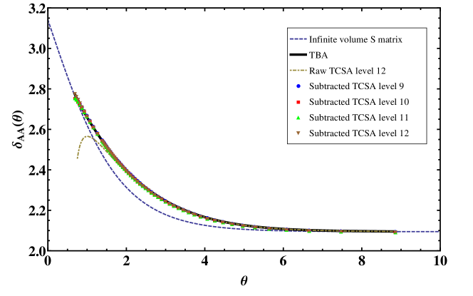
Figure 5.5: (color online) Comparing $\delta_{AA}(\theta)$ extracted from the first excited TCSA level in sectors $\mathcal{H}_{\pm}$ in the paramagnetic phase (lowest lying $AA$/$\bar{A}\bar{A}$ state) to the scattering theory predictions (4.18) and to TBA.

Note that the deviation of the TCSA phase-shift in the high energy (small volume) regime is fully explained by TBA, which is not very surprising in view of the excellent agreement between TCSA and TBA demonstrated in Appendix C. For low energies (large volumes) the agreement is very much improved by the renormalization procedure. We also demonstrate that the residual cut-off dependence is practically nonexistent except for very low energies; the remaining deviation in that regime is expected to be due to $O(\lambda^{3})$ cut-off effects, the elimination of which would necessitate the extension of the renormalization procedure to higher order.

6 Discussion and outlook

In this paper we provided a description of the finite volume spectrum of the scaling Potts model combining two approaches: the renormalized TCSA, the idea of which goes back to the recent papers [6, 8, 9], and an excited TBA system which was first proposed in the present work. We have developed the general theory of cut-off dependence and counter terms for energy levels in TCSA, and applied it to the scaling Potts field theory. Using comparison with the TBA predictions we have shown that this gives a very precise tool to study the finite size spectrum of perturbed conformal field theory.

There are several potential applications of the results presented here. TCSA has recent been extended to asymptotically free field theories [25], but this line of development is still in its infancy. In fact, a systematic understanding of the construction of counter terms should prove very useful in this context. Another possible application is given the application of the truncation approach to study non-equilibrium physics in condensed matter theory [28]. In addition, integrability, finite size effects and the ideas of perturbed conformal field theory have also appeared in the AdS/CFT correspondence (cf. [29] and references therein). We expect that the methods developed here can be useful for these applications both by improving numerical reliability and providing a detailed understanding of scale dependence.

There is also an interesting implication of the present results for the study of the quantum Potts spin chain. In [30] perturbative calculations supplemented with renormalization group arguments cast some doubt on the applicability of the factorized scattering amplitudes in long-distance limit of the spin chain. A detailed DMRG analysis has shown that the observed discrepancy between the factorized S matrix and the low-energy scattering of quasi-particles in the discrete spin chain persists even non-perturbatively [31], and it was speculated that this was due to the presence of an irrelevant operator that has a large effect on the low-energy limit of the scattering amplitudes away from the scaling limit. In this connection, first of all we note that the raw TCSA phase-shifts in figures 5.3, 5.4 and 5.5 show a characteristic deviation from the field theory predictions at low energies which is very similar to that observed in the DMRG results of [31]. In contrast to the DMRG study, in this paper we are in a position to identify the source of this deviation: it originates from the cut-off dependence introduced by the operators that appear in the OPE

$$\Phi_{2,1}(z,\bar{z})\Phi_{2,1}(0,0)=\frac{1}{(z\bar{z}){}^{4/5}}\left(\mathbb{I}+h_{2.1}^{2}\,(z\bar{z})^{2}(T\bar{T})(0,0)+\dots\right)+C_{\Phi_{2,1}\Phi_{2,1}}^{\Phi_{3,1}}\,(z\bar{z})^{3/5}\left(\Phi_{3,1}(0,0)+\dots\right)$$

The counter term from the identity $\mathbb{I}$ is the universal contribution shown explicitly in (3.74), which only renormalizes the bulk energy density and thus makes no contribution to the extracted phase-shifts. Therefore the dominant part of the cut-off dependence comes from the irrelevant operators: the leading one is $\Phi_{3,1}$ , while the first subleading one is $T\bar{T}$. Once the counter-terms are added, all cut-off dependence is eliminated to order $\lambda^{2}$ and the phase-shifts indeed show a much better agreement with the field theoretical predictions. In TCSA it is therefore clear that the cut-off dependence comes from irrelevant operators, which makes it very plausible that the very similar effect noticed in the DMRG data is also a result of the contribution of the same irrelevant operators. Note also that the cut-off dependence still remains for lower energies, which correspond to larger values of the volume and therefore larger $\lambda$. Therefore it is clear that these effects can only be removed by considering the counter terms at higher order, which is out of the scope of this paper. To sum up, our results for the cut-off dependence in the TCSA approach strongly supports that the similar effect in the spin chain is caused by the same irrelevant operators. A detailed matching of the phenomenology of the spin chain with the perturbed CFT extended with irrelevant operators, however, needs better quality data for the spin chain than presently available, in addition to evaluating the counter terms for the perturbed CFT Hamiltonian extended with the irrelevant fields.

Another interesting line of development is to extend the theory of counter terms to a full renormalization group description along the lines in [6, 7, 9]. The perturbing operator considered in these works had an OPE of the form

$$\Phi\Phi\sim\mathbb{I}+\Phi$$

leading to a running coupling at order $\lambda^{2}$. We note that at the next order the perturbing operator $\Phi_{2,1}$ appears in the triple product of itself, which leads to a running coupling at order $\lambda^{3}$. However, even at second order there appear running couplings in the Potts field theory when other perturbing operators are added, such as in the work [5]. We are planning to return to these issues in the near future.

Acknowledgments

The authors acknowledge very useful discussions with G. Watts. This work was supported by the Momentum grant LP2012-50/2013 of the Hungarian Academy of Sciences.

Appendix A CFT data

A.1 Conformal blocks

The conformal blocks needed in this work are known in a closed form for the Potts model [17]. Below we summarize the necessary data for the renormalization computations. Considering the following correlators

$$\langle\Phi_{r,s}|\Phi_{2,1}(1)\Phi_{2,1}(z)|\Phi_{r,s}\rangle$$ (A.1)

the conformal blocks forming a basis for their chiral part around $z=0$ are

(A.2)

where the small $\phi$s refer to the chiral components, and

$$\,{}_{2}F_{1}\left(\alpha,\beta;\gamma\big{|}z\right)$$ (A.3)

denotes the standard hypergeometric function. The basis for the conformal blocks around $z=1$ is given by

For clarity of conventions, the insertion points of the fields were displayed above; in the following considerations they are suppressed. Denoting $\Phi=\Phi_{2,1}$ and its chiral part by $\phi=\phi_{2,1}$ , the two bases are related by the following duality relations

where

$$\mathcal{F}_{jk}[i]=F_{jk}\left[\begin{array}[]{cc}\phi&\phi\\ i&i\end{array}\right]$$ (A.6)

are the so-called fusion coefficients. These can be easily obtained using the transformation formulas obeyed by the hypergeometric functions. The ones relevant for our calculations are

$$\mathcal{F}_{\phi_{r-1,s}\mathbb{I}}[\phi_{r,s}] = -\frac{2\sqrt{\frac{2}{5+\sqrt{5}}}\pi\Gamma\left(-\frac{6r}{5}+s+1\right)}{\Gamma\left(-\frac{2}{5}\right)\Gamma\left(\frac{6}{5}\right)\Gamma\left(-\frac{6r}{5}+s+\frac{6}{5}\right)}$$

$$\mathcal{F}_{\phi_{r-1,s}\phi_{3,1}}[\phi_{r,s}] = \frac{2\sqrt{\frac{2}{5+\sqrt{5}}}\pi\Gamma\left(-\frac{6r}{5}+s+1\right)}{\Gamma\left(-\frac{1}{5}\right)\Gamma\left(\frac{12}{5}\right)\Gamma\left(-\frac{6r}{5}+s-\frac{1}{5}\right)}$$

$$\mathcal{F}_{\phi_{r+1,s}\mathbb{I}}[\phi_{r,s}] = -\frac{2\sqrt{\frac{2}{5+\sqrt{5}}}\pi\Gamma\left(\frac{6r}{5}-s+1\right)}{\Gamma\left(-\frac{2}{5}\right)\Gamma\left(\frac{6}{5}\right)\Gamma\left(\frac{6r}{5}-s+\frac{6}{5}\right)}$$

$$\mathcal{F}_{\phi_{r+1,s}\phi_{3,1}}[\phi_{r,s}] = \frac{2\sqrt{\frac{2}{5+\sqrt{5}}}\pi\Gamma\left(\frac{6r}{5}-s+1\right)}{\Gamma\left(-\frac{1}{5}\right)\Gamma\left(\frac{12}{5}\right)\Gamma\left(\frac{6r}{5}-s-\frac{1}{5}\right)}$$ (A.7)

Another necessary ingredient is the expansion of the blocks (LABEL:eq:crossed_channel_block) around $z=1$. One way this can be calculated is computing the series expansion of the conformal blocks using the Taylor series of the hypergeometric function and the binomial series.

On the other hand, a model independent way to obtain the expansion is provided by Virasoro symmetry. Recalling the notations in (3.56)

(A.10)

the first few coefficients can be easily obtained using the conformal Ward identities, which give the following commutation relations between the Virasoro generators and the primary fields:

$$\left[L_{n}\left(z\right),\Phi\left(w,\bar{w}\right)\right] = h\left(n+1\right)\left(w-z\right)^{n}\Phi\left(w,\bar{w}\right)+\left(w-z\right)^{n+1}\partial_{w}\Phi\left(w,\bar{w}\right)$$

$$\left[\bar{L}_{n}\left(\bar{z}\right),\Phi\left(w,\bar{w}\right)\right] = \bar{h}\left(n+1\right)\left(\bar{w}-\bar{z}\right)^{n}\Phi\left(w,\bar{w}\right)+\left(\bar{w}-\bar{z}\right)^{n+1}\partial_{\bar{w}}\Phi\left(w,\bar{w}\right)$$ (A.12)

where

$$L_{n}(z)=\oint_{z}\frac{d\zeta}{2\pi i}\left(\zeta-z\right)^{n+1}T(\zeta)\qquad\bar{L}_{n}(\bar{z})=\oint_{\bar{z}}\frac{d\bar{\zeta}}{2\pi i}\left(\bar{\zeta}-\bar{z}\right)^{n+1}\bar{T}(\bar{\zeta})$$ (A.13)

are the modes of the conformal energy momentum tensor located at $(z,\bar{z})$; the modes located at $z=\infty$ are given by

$$L_{n}(\infty)=-\oint_{\infty}\frac{d\zeta}{2\pi i}\zeta^{-n+1}T(\zeta)=L_{-n}(0)\qquad\bar{L}_{n}(\infty)=-\oint_{\infty}\frac{d\bar{\zeta}}{2\pi i}\bar{\zeta}^{-n+1}\bar{T}(\bar{\zeta})=\bar{L}_{-n}(0)$$ (A.14)

We computed the block coefficients up to $r=5$, but for the sake of brevity we only give the first three cases:

$$B_{0}\left[\begin{array}[]{cc}j&j\\ i&i\end{array}k\right] = 1$$ (A.17)

$$B_{1}\left[\begin{array}[]{cc}j&j\\ i&i\end{array}k\right] = \frac{h_{k}}{2}$$ (A.20)

$$B_{2}\left[\begin{array}[]{cc}j&j\\ i&i\end{array}k\right] = \frac{h_{k}\left[(c+8)h_{k}^{2}+2(c-4)h_{k}+c+4h_{j}(h_{k}-1)+8h_{k}^{3}\right]+4h_{i}\left[h_{j}(4h_{k}+2)+\left(h_{k}-1\right)h_{k}\right]}{4\left(2(c-5)h_{k}+c+16h_{k}^{2}\right)}$$ (A.23)

where $h_{i}$,$h_{j}$ and $h_{k}$ are the conformal weights of the respective fields.

For descendant state calculations we consider the first level only, as this is all we need in the main text. The duality relations have the same fusion coefficients

and the conformal blocks in the dual channel can be expanded as

(A.27)

where we computed the coefficients up to $r=5$. The first three of them are

$$B_{0}\left[\begin{array}[]{cc}j&j\\ L_{-1}i&L_{-1}i\end{array}k\right] = 2h_{i}+h_{k}^{2}-h_{k}$$ (A.31)

$$B_{1}\left[\begin{array}[]{cc}j&j\\ L_{-1}i&L_{-1}i\end{array}k\right] = \frac{1}{2}h_{k}\left(2h_{i}+h_{k}^{2}-h_{k}\right)$$ (A.34)

$$B_{2}\left[\begin{array}[]{cc}j&j\\ L_{-1}i&L_{-1}i\end{array}k\right] = \frac{h_{k}\left(h_{k}^{2}-1\right)\left(h_{k}\left(ch_{k}+c+8h_{k}^{2}-4\right)+4h_{j}\left(h_{k}+2\right)\right)+8h_{i}^{2}\left(h_{j}\left(4h_{k}+2\right)+\left(h_{k}-1\right)h_{k}\right)}{4\left(2(c-5)h_{k}+c+16h_{k}^{2}\right)}$$

$$+ \frac{h_{i}\left(h_{k}\left((c+12)h_{k}^{2}+2(c-5)h_{k}+c+10h_{k}^{3}-4\right)+8h_{j}\left(h_{k}^{3}+4h_{k}^{2}+3h_{k}+1\right)\right)}{2\left(2(c-5)h_{k}+c+16h_{k}^{2}\right)}$$

A.2 Structure constants

For reference, here we list the matrix elements of the field $\Phi_{\frac{2}{5},\frac{2}{5}}$ between the primary states of the Hilbert space (2.15). These can be arranged by the four sectors (2.34), as matrix elements between different sectors vanish. The full set of structure constants can be obtained from [33]; here we present them in a basis of states which is orthonormal.

In the sector $\mathcal{H}_{0}=\mathcal{S}_{0,0}\oplus\mathcal{S}_{\frac{2}{5},\frac{2}{5}}\oplus\mathcal{S}_{\frac{7}{5},\frac{7}{5}}\oplus\mathcal{S}_{3,3}$, the matrix of $\Phi_{\frac{2}{5},\frac{2}{5}}(1,1)$ on the basis of primary states (ordered the same way as the modules) is

$$\left(\begin{array}[]{cccc}0&1&0&0\\ 1&0&0.9363044884&0\\ 0&0.9363044884&0&0.8076923077\\ 0&0&0.8076923077&0\end{array}\right)$$ (A.38)

In both sectors $\mathcal{H}_{\pm}=\mathcal{S}_{\frac{1}{15},\frac{1}{15}}^{\pm}\oplus\mathcal{S}_{\frac{2}{3},\frac{2}{3}}^{\pm}$ one has

$$\left(\begin{array}[]{cc}0.5461776182&2/3\\ 2/3&0\end{array}\right)$$ (A.39)

while in $\mathcal{H}_{1}=\mathcal{S}_{\frac{2}{5},\frac{7}{5}}\oplus\mathcal{S}_{\frac{7}{5},\frac{2}{5}}\oplus\mathcal{S}_{0,3}\oplus\mathcal{S}_{3,0}$ the matrix elements are

$$\left(\begin{array}[]{cccc}0&0.9363044884&0.8987170343&0\\ 0.9363044884&0&0&0.8987170343\\ 0.8987170343&0&0&0\\ 0&0.8987170343&0&0\end{array}\right)$$ (A.40)

The above structure constants are in one-to-one correspondence with the operator product coefficients involving the field $\Phi=\Phi_{\frac{2}{5},\frac{2}{5}}$. Writing the operator product expansion in the form

$$\Phi_{\frac{2}{5},\frac{2}{5}}(z,z)A(0,0)=\sum_{B}C_{\Phi A}^{B}\frac{B(0,0)}{z^{h_{A}+2/5-h_{B}}\bar{z}^{\bar{h}_{A}+2/5-\bar{h}_{B}}}$$ (A.41)

the OPE coefficients are

$$C_{\Phi A}^{B}=\langle B|\Phi_{\frac{2}{5},\frac{2}{5}}(1,1)|A\rangle$$ (A.42)

For primary states, these coefficients are given above in (A.38,A.39,A.40); for descendant states they be constructed from the primary ones by a recursive application of the conformal Ward identities (A.12).

Appendix B Derivation of the UV limit of the excited Potts TBA

Let us introduce a short-hand notation for the source terms

$$g(\theta|\theta^{+},\theta^{-}) = \sum_{k=1}^{N^{+}}\log\frac{S_{1}(\theta-\theta_{k}^{+})}{S_{2}(\theta-\bar{\theta}_{k}^{+})}+\sum_{l=1}^{N^{-}}\log\frac{S_{2}(\theta-\theta_{l}^{-})}{S_{1}(\theta-\bar{\theta}_{l}^{-})}$$

$$\bar{g}(\theta|\theta^{+},\theta^{-}) = \sum_{k=1}^{N^{+}}\log\frac{S_{2}(\theta-\theta_{k}^{+})}{S_{1}(\theta-\bar{\theta}_{k}^{+})}+\sum_{l=1}^{N^{-}}\log\frac{S_{1}(\theta-\theta_{l}^{-})}{S_{2}(\theta-\bar{\theta}_{l}^{-})}$$

so that we can write the TBA equations in the form

$$\epsilon_{1}(\theta) = i\omega+mR\cosh\theta+g(\theta|\theta^{+},\theta^{-})-\phi_{1}\star L_{1}(\theta)-\phi_{2}\star L_{2}(\theta)$$

$$\epsilon_{2}(\theta) = -i\omega+mR\cosh\theta+\bar{g}(\theta|\theta^{+},\theta^{-})-\phi_{1}\star L_{2}(\theta)-\phi_{2}\star L_{1}(\theta)$$

$$e^{\epsilon_{1}(\theta_{k}^{+})}=e^{\epsilon_{1}(\bar{\theta}_{k}^{-})}=-1$$

$$e^{\epsilon_{2}(\theta_{k}^{-})}=e^{\epsilon_{2}(\bar{\theta}_{k}^{+})}=-1$$

$$E(R) = -im\sum_{k}\left(\sinh\theta_{k}^{+}-\sinh\bar{\theta}_{k}^{+}\right)-im\sum_{l}\left(\sinh\theta_{l}^{-}-\sinh\bar{\theta}_{l}^{-}\right)-\int\frac{d\theta}{2\pi}m\cosh\theta\,\left(L_{1}(\theta)+L_{2}(\theta)\right)$$

where the twist parameter can take the values where

$$\omega=\frac{2\pi}{3}n_{\omega}\qquad n_{\omega}=-1,0,+1$$ (B.1)

We only derive the right-moving conformal behaviour; the left-moving part can be obtained in a similar way. For $mR\ll 1$ the right kink limit of the TBA is obtained by redefining

$$\theta\rightarrow\theta-\log\frac{1}{mR}$$ (B.2)

and similarly for the positions of the sources

$$\theta_{k}^{\pm}\rightarrow\theta_{k}^{\pm}-\log\frac{1}{mR}\qquad\bar{\theta}_{k}^{\pm}\rightarrow\bar{\theta}_{k}^{\pm}-\log\frac{1}{mR}$$ (B.3)

Those sources whose positions remain finite in the limit are called right movers. To obtain the limit of the source terms, one can compute

$$\lim_{\theta\rightarrow+\infty}\log\frac{S_{1}(\theta-\theta_{k}^{+})}{S_{2}(\theta-\bar{\theta}_{k}^{+})}=-\frac{2\pi}{3}i \lim_{\theta\rightarrow-\infty}\log\frac{S_{1}(\theta-\theta_{k}^{-})}{S_{2}(\theta-\bar{\theta}_{k}^{-})}=\frac{2\pi}{3}i$$

$$\lim_{\theta\rightarrow+\infty}\log\frac{S_{2}(\theta-\theta_{k}^{+})}{S_{1}(\theta-\bar{\theta}_{k}^{+})}=\frac{2\pi}{3}i \lim_{\theta\rightarrow-\infty}\log\frac{S_{2}(\theta-\theta_{k}^{+})}{S_{1}(\theta-\bar{\theta}_{k}^{+})}=-\frac{2\pi}{3}i$$ (B.4)

Taking the limit $mR\rightarrow 0$ we get that the right kink limiting functions

$$\epsilon_{i}^{R}(\theta)=\lim_{R\rightarrow 0}\epsilon_{i}(\theta-\log mR)$$ (B.5)

satisfy the equations

$$\epsilon_{1}^{R}(\theta) = \frac{1}{2}e^{\theta}+i\omega_{R}+g_{R}(\theta|\theta^{+},\theta^{-})-\phi_{1}\star L_{1}(\theta)-\phi_{2}\star L_{2}(\theta)$$

$$\epsilon_{2}^{R}(\theta) = \frac{1}{2}e^{\theta}-i\omega_{R}+\bar{g}_{R}(\theta|\theta^{+},\theta^{-})-\phi_{1}\star L_{2}(\theta)-\phi_{2}\star L_{1}(\theta)$$

$$\epsilon_{1}^{R}(\theta_{k}^{+}) = i\pi\left(2n_{k}^{+}+1\right)$$

$$\epsilon_{2}^{R}(\theta_{l}^{-}) = i\pi\left(2n_{l}^{+}+1\right)$$ (B.6)

where

$$g_{R}(\theta|\theta^{+},\theta^{-}) = \sum_{k=1}^{N_{R}^{+}}\log\frac{S_{1}(\theta-\theta_{k}^{+})}{S_{2}(\theta-\bar{\theta}_{k}^{+})}+\sum_{l=1}^{N_{R}^{-}}\log\frac{S_{2}(\theta-\theta_{l}^{-})}{S_{1}(\theta-\bar{\theta}_{l}^{-})}$$

$$\bar{g}_{R}(\theta|\theta^{+},\theta^{-}) = \sum_{k=1}^{N_{R}^{+}}\log\frac{S_{2}(\theta-\theta_{k}^{+})}{S_{1}(\theta-\bar{\theta}_{k}^{+})}+\sum_{l=1}^{N_{R}^{-}}\log\frac{S_{1}(\theta-\theta_{l}^{-})}{S_{2}(\theta-\bar{\theta}_{l}^{-})}$$ (B.7)

with sums only over the right-movers, and the effective right twist is

$$\omega_{R}=\omega+\frac{2\pi}{3}\left[\left(N^{-}-N_{R}^{-}\right)-\left(N^{+}-N_{R}^{+}\right)\right]$$ (B.8)

The right handed component of the effective central charge can be written as

$$c_{R}=\frac{6}{2\pi}i\sum_{k=1}^{N_{R}^{+}}\left(e^{\theta_{k}^{+}}-e^{\bar{\theta}_{k}^{+}}\right)+\frac{6}{2\pi}i\sum_{l=1}^{N_{R}^{-}}\left(e^{\theta_{l}^{-}}-e^{\bar{\theta}_{l}^{-}}\right)+\frac{3}{\pi^{2}}\int d\theta\frac{e^{\theta}}{2}\,\left(L_{1}(\theta)+L_{2}(\theta)\right)$$ (B.9)

We can rewrite these equations in the following form

$$\epsilon_{1}^{R}(\theta) = \frac{1}{2}e^{\theta}+i\omega_{R}-2i\pi m_{R}+g_{R}(\theta|\theta^{+},\theta^{-})-\phi_{1}\star L_{1}(\theta)-\phi_{2}\star L_{2}(\theta)$$

$$\epsilon_{2}^{R}(\theta) = \frac{1}{2}e^{\theta}-i\omega_{R}+2i\pi m_{R}+\bar{g}_{R}(\theta|\theta^{+},\theta^{-})-\phi_{1}\star L_{2}(\theta)-\phi_{2}\star L_{1}(\theta)$$

$$\epsilon_{1}^{R}(\theta_{k}^{+}) = i\pi\left(2n_{k}^{+}-2m_{R}+1\right)$$

$$\epsilon_{2}^{R}(\theta_{l}^{-}) = i\pi\left(2n_{l}^{+}-2m_{R}+1\right)$$ (B.10)

where $m_{R}$ is defined from

$$i\omega_{R}+\lim_{\theta\rightarrow-\infty}g_{R}\left(\theta|\theta^{+},\theta^{-}\right) = i\frac{2\pi}{3}\left[n_{\omega}+\left(N^{-}-N_{R}^{-}\right)-\left(N^{+}-N_{R}^{+}\right)-N_{R}^{-}+N_{R}^{+}\right]$$ (B.11)

$$= i\frac{2\pi}{3}\left(3m_{R}+\tilde{n}_{\omega}\right)$$

where $m_{R}$ is an integer and $\tilde{n}_{\omega}=0$ or $\pm 1$ is the remainder. One can the use the standard dilogarithm trick [10, 13] to write

$$\frac{1}{2}e^{\theta} = \epsilon_{1}^{R}(\theta)-i\omega_{R}+2i\pi m_{R}-g_{R}(\theta|\theta^{+},\theta^{-})+\phi_{1}\star L_{1}(\theta)+\phi_{2}\star L_{2}(\theta)$$

$$\frac{1}{2}e^{\theta} = \epsilon_{2}^{R}(\theta)+i\omega_{R}-2i\pi m_{R}-\bar{g}_{R}(\theta|\theta^{+},\theta^{-})+\phi_{1}\star L_{2}(\theta)+\phi_{2}\star L_{1}(\theta)$$ (B.12)

Differentiating the two sides

$$\frac{1}{2}e^{\theta} = \frac{d}{d\theta}\left\{\epsilon_{1}^{R}(\theta)-g_{R}(\theta|\theta^{+},\theta^{-})+\phi_{1}\star L_{1}(\theta)+\phi_{2}\star L_{2}(\theta)\right\}$$

$$\frac{1}{2}e^{\theta} = \frac{d}{d\theta}\left\{\epsilon_{2}^{R}(\theta)-\bar{g}_{R}(\theta|\theta^{+},\theta^{-})+\phi_{1}\star L_{2}(\theta)+\phi_{2}\star L_{1}(\theta)\right\}$$ (B.13)

and substituting into the expression (B.9) we obtain

$$c_{R} = \frac{6}{2\pi}i\sum_{k=1}^{N_{R}^{+}}\left(e^{\theta_{k}^{+}}-e^{\bar{\theta}_{k}^{+}}\right)+\frac{6}{2\pi}i\sum_{l=1}^{N_{R}^{-}}\left(e^{\theta_{l}^{-}}-e^{\bar{\theta}_{l}^{-}}\right)$$ (B.14)

$$+\frac{3}{\pi^{2}}\int d\theta\frac{d}{d\theta}\left\{\epsilon_{1}^{R}(\theta)-g_{R}(\theta|\theta^{+},\theta^{-})+\phi_{1}\star L_{1}(\theta)+\phi_{2}\star L_{2}(\theta)\right\}\,L_{1}(\theta)$$

$$+\frac{3}{\pi^{2}}\int d\theta\frac{d}{d\theta}\left\{\epsilon_{2}^{R}(\theta)-\bar{g}_{R}(\theta|\theta^{+},\theta^{-})+\phi_{1}\star L_{2}(\theta)+\phi_{2}\star L_{1}(\theta)\right\}\,L_{2}(\theta)$$

$$= \frac{6}{2\pi}i\sum_{k=1}^{N_{R}^{+}}\left(e^{\theta_{k}^{+}}-e^{\bar{\theta}_{k}^{+}}\right)+\frac{6}{2\pi}i\sum_{l=1}^{N_{R}^{-}}\left(e^{\theta_{l}^{-}}-e^{\bar{\theta}_{l}^{-}}\right)$$

$$+\frac{3}{\pi^{2}}\int_{\epsilon_{1}^{R}(-\infty)}^{+\infty}d\epsilon\log(1+e^{-\epsilon})+\frac{6}{\pi^{2}}\int_{\epsilon_{2}^{R}(-\infty)}^{+\infty}d\epsilon\log(1+e^{-\epsilon})$$

$$+\frac{3}{\pi^{2}}\int d\theta\frac{d}{d\theta}\left\{-g_{R}(\theta|\theta^{+},\theta^{-})+\phi_{1}\star L_{1}(\theta)+\phi_{2}\star L_{2}(\theta)\right\}\,L_{1}(\theta)$$

$$+\frac{3}{\pi^{2}}\int d\theta\frac{d}{d\theta}\left\{-\bar{g}_{R}(\theta|\theta^{+},\theta^{-})+\phi_{1}\star L_{2}(\theta)+\phi_{2}\star L_{1}(\theta)\right\}\,L_{2}(\theta)$$

where the integrals over $\epsilon$ must be taken over an appropriate contour in the $\epsilon$ plane which is analytically equivalent the curves $\epsilon_{i}^{R}(\theta)$ as $\theta$ runs over the real line.

In the next step, we can treat the $\theta$ integrals using partial integration:

$$\int d\theta\frac{d}{d\theta}\left\{-g_{R}(\theta|\theta^{+},\theta^{-})+\phi_{1}\star L_{1}(\theta)+\phi_{2}\star L_{2}(\theta)\right\}\,L_{1}(\theta)$$ (B.15)

$$+\int d\theta\frac{d}{d\theta}\left\{-\bar{g}_{R}(\theta|\theta^{+},\theta^{-})+\phi_{1}\star L_{2}(\theta)+\phi_{2}\star L_{1}(\theta)\right\}\,L_{2}(\theta)$$

$$= \int d\theta\left\{-g_{R}^{\prime}(\theta|\theta^{+},\theta^{-})L_{1}(\theta)-\bar{g}_{R}^{\prime}(\theta|\theta^{+},\theta^{-})L_{2}(\theta)\right\}$$

$$-\int d\theta\left\{\phi_{1}\star L_{1}(\theta)+\phi_{2}\star L_{2}(\theta)\right\}\,L_{1}^{\prime}(\theta)$$

$$-\int d\theta\left\{\phi_{1}\star L_{2}(\theta)+\phi_{2}\star L_{1}(\theta)\right\}\,L_{2}^{\prime}(\theta)$$

$$+\left[\left\{\phi_{1}\star L_{1}(\theta)+\phi_{2}\star L_{2}(\theta)\right\}\,L_{1}(\theta)\right]_{-\infty}^{\infty}$$

$$+\left[\left\{\phi_{1}\star L_{2}(\theta)+\phi_{2}\star L_{1}(\theta)\right\}\,L_{2}(\theta)\right]_{-\infty}^{\infty}$$

and the fact that $L_{1,2}(\infty)=0$ to obtain

$$c_{R} = \frac{6}{2\pi}i\sum_{k=1}^{N_{R}^{+}}\left(e^{\theta_{k}^{+}}-e^{\bar{\theta}_{k}^{+}}\right)+\frac{6}{2\pi}i\sum_{l=1}^{N_{R}^{-}}\left(e^{\theta_{l}^{-}}-e^{\bar{\theta}_{l}^{-}}\right)$$ (B.16)

$$+\frac{3}{\pi^{2}}\int_{\epsilon_{1}^{R}(-\infty)}^{+\infty}d\epsilon\log(1+e^{-\epsilon})+\frac{3}{\pi^{2}}\int_{\epsilon_{2}^{R}(-\infty)}^{+\infty}d\epsilon\log(1+e^{-\epsilon})$$

$$+\frac{3}{\pi^{2}}\int d\theta\left\{-g_{R}^{\prime}(\theta|\theta^{+},\theta^{-})L_{1}(\theta)-\bar{g}_{R}^{\prime}(\theta|\theta^{+},\theta^{-})L_{2}(\theta)\right\}$$

$$-\frac{3}{\pi^{2}}\frac{1}{2}\left[\phi_{1}\star L_{1}(-\infty)+\phi_{2}\star L_{2}(-\infty)\right]\,L_{1}(-\infty)$$

$$-\frac{3}{\pi^{2}}\frac{1}{2}\left[\phi_{1}\star L_{2}(-\infty)+\phi_{2}\star L_{2}(-\infty)\right]\,L_{2}(-\infty)$$

The remaining integrals can be expressed using the kink TBA equations for $\theta\rightarrow-\infty$:

$$\phi_{1}\star L_{1}(-\infty)+\phi_{2}\star L_{2}(-\infty) = -\epsilon_{1}^{R}(-\infty)+i\omega_{R}-2i\pi m_{R}+g_{R}(-\infty|\theta^{+},\theta^{-})$$

$$\phi_{1}\star L_{2}(-\infty)+\phi_{2}\star L_{1}(-\infty) = -\epsilon_{2}^{R}(-\infty)-i\omega_{R}+2i\pi m_{R}+\bar{g}_{R}(-\infty|\theta^{+},\theta^{-})$$ (B.17)

Using the definition of $m_{R}$ leads to

$$\phi_{1}\star L_{1}(-\infty)+\phi_{2}\star L_{2}(-\infty) = -\epsilon_{1}^{R}(-\infty)+i\frac{2\pi}{3}\tilde{n}_{\omega}$$

$$\phi_{1}\star L_{2}(-\infty)+\phi_{2}\star L_{1}(-\infty) = -\epsilon_{2}^{R}(-\infty)-i\frac{2\pi}{3}\tilde{n}_{\omega}$$ (B.18)

For the terms involving $g_{R}^{\prime}$ and $\bar{g}_{R}^{\prime}$ we can write

$$g_{R}^{\prime}(\theta|\theta^{+},\theta^{-}) = \sum_{k=1}^{N_{R}^{+}}i\phi_{1}(\theta-\theta_{k}^{+})-i\phi_{2}(\theta-\bar{\theta}_{k}^{+})+\sum_{l=1}^{N_{R}^{-}}i\phi_{2}(\theta-\theta_{l}^{-})-i\phi_{1}(\theta-\bar{\theta}_{l}^{-})$$

$$\bar{g}_{R}^{\prime}(\theta|\theta^{+},\theta^{-}) = \sum_{k=1}^{N_{R}^{+}}i\phi_{2}(\theta-\theta_{k}^{+})-i\phi_{1}(\theta-\bar{\theta}_{k}^{+})+\sum_{l=1}^{N_{R}^{-}}i\phi_{1}(\theta-\theta_{l}^{-})-i\phi_{2}(\theta-\bar{\theta}_{l}^{-})$$ (B.19)

and so

$$\int d\theta\left\{-g_{R}^{\prime}(\theta|\theta^{+},\theta^{-})L_{1}(\theta)-\bar{g}_{R}^{\prime}(\theta|\theta^{+},\theta^{-})L_{2}(\theta)\right\}$$ (B.20)

$$= -2\pi i\sum_{k=1}^{N_{R}^{+}}\left\{\phi_{1}\star L_{1}(\theta_{k}^{+})+\phi_{2}\star L_{2}(\theta_{k}^{+})-\phi_{2}\star L_{1}(\bar{\theta}_{k}^{+})-\phi_{1}\star L_{2}(\bar{\theta}_{k}^{+})\right\}$$

$$-2\pi i\sum_{l=1}^{N_{R}^{-}}\left\{-\phi_{1}\star L_{1}(\bar{\theta}_{l}^{-})-\phi_{2}\star L_{2}(\bar{\theta}_{l}^{-})+\phi_{2}\star L_{1}(\theta_{l}^{-})+\phi_{1}\star L_{2}(\theta_{l}^{-})\right\}$$

Now we can eliminate the convolution terms using the equations determining the singularity positions

$$i\pi\left(2n_{k}^{+}+1\right) = \frac{1}{2}e^{\theta_{k}^{+}}+i\omega_{R}+g_{R}(\theta_{k}^{+}|\theta^{+},\theta^{-})-\phi_{1}\star L_{1}(\theta_{k}^{+})-\phi_{2}\star L_{2}(\theta_{k}^{+})$$

$$-i\pi\left(2n_{k}^{+}+1\right) = \frac{1}{2}e^{\bar{\theta}_{k}^{+}}-i\omega_{R}+\bar{g}_{R}(\bar{\theta}_{k}^{+}|\theta^{+},\theta^{-})-\phi_{1}\star L_{2}(\bar{\theta}_{k}^{+})-\phi_{2}\star L_{1}(\bar{\theta}_{k}^{+})$$ (B.21)

$$-i\pi\left(2n_{l}^{-}+1\right) = \frac{1}{2}e^{\bar{\theta}_{l}^{-}}+i\omega_{R}+g_{R}(\bar{\theta}_{l}^{-}|\theta^{+},\theta^{-})-\phi_{1}\star L_{1}(\bar{\theta}_{l}^{-})-\phi_{2}\star L_{2}(\bar{\theta}_{l}^{-})$$

$$i\pi\left(2n_{l}^{-}+1\right) = \frac{1}{2}e^{\theta_{l}^{-}}-i\omega_{R}+\bar{g}_{R}(\theta_{l}^{-}|\theta^{+},\theta^{-})-\phi_{1}\star L_{2}(\theta_{l}^{-})-\phi_{2}\star L_{1}(\theta_{l}^{-})$$ (B.22)

The end result is

$$c_{R} = \frac{3}{\pi^{2}}\left\{\int_{\epsilon_{1}^{R}(-\infty)}^{+\infty}d\epsilon\log(1+e^{-\epsilon})\right\}+\frac{3}{\pi^{2}}\left\{\int_{\epsilon_{2}^{R}(-\infty)}^{+\infty}d\epsilon\log(1+e^{-\epsilon})\right\}$$ (B.23)

$$-12\sum_{k=1}^{N_{R}^{+}}\left(2n_{k}^{+}+1\right)-12\sum_{l=1}^{N_{R}^{-}}\left(2n_{l}^{-}+1\right)+\frac{12}{\pi}\omega_{R}\left(N_{R}^{+}-N_{R}^{-}\right)$$

$$-\frac{6}{\pi}i\sum_{k=1}^{N_{R}^{+}}\left\{g_{R}(\theta_{k}^{+}|\theta^{+},\theta^{-})-\bar{g}_{R}(\bar{\theta}_{k}^{+}|\theta^{+},\theta^{-})\right\}-\frac{6}{\pi}i\sum_{l=1}^{N_{R}^{-}}\left\{\bar{g}_{R}(\bar{\theta}_{l}^{-}|\theta^{+},\theta^{-})-g_{R}(\theta_{l}^{-}|\theta^{+},\theta^{-})\right\}$$

$$-\frac{3}{\pi^{2}}\frac{1}{2}\left[-\log Y_{1}+i\frac{2\pi}{3}\tilde{n}_{\omega}\right]\,\log\left(1+Y_{1}^{-1}\right)-\frac{3}{\pi^{2}}\frac{1}{2}\left[-\log Y_{2}-i\frac{2\pi}{3}\tilde{n}_{\omega}\right]\,\log\left(1+Y_{2}^{-1}\right)$$

where $Y_{i}=\epsilon_{i}\left(-\infty\right)$ are solutions of the plateau equation

$$\log Y_{1} = i\frac{2\pi}{3}\tilde{n}_{\omega}+\frac{1}{3}\log\left(1+Y_{1}^{-1}\right)+\frac{2}{3}\log\left(1+Y_{2}^{-1}\right)$$

$$\log Y_{2} = -i\frac{2\pi}{3}\tilde{n}_{\omega}+\frac{2}{3}\log\left(1+Y_{1}^{-1}\right)+\frac{1}{3}\log\left(1+Y_{2}^{-1}\right)$$ (B.24)

From [11, 12], the solutions of these equations are known, together with the values of the dilogarithm integrals:

$$\frac{3}{\pi^{2}}\left\{\int_{\epsilon_{1}^{R}(-\infty)}^{+\infty}d\epsilon\log(1+e^{-\epsilon})\right\}+\frac{3}{\pi^{2}}\left\{\int_{\epsilon_{2}^{R}(-\infty)}^{+\infty}d\epsilon\log(1+e^{-\epsilon})\right\}$$

$$-\frac{3}{\pi^{2}}\frac{1}{2}\left[-\log Y_{1}+i\frac{2\pi}{3}\tilde{n}_{\omega}\right]\,\log\left(1+Y_{1}^{-1}\right)-\frac{3}{\pi^{2}}\frac{1}{2}\left[-\log Y_{2}-i\frac{2\pi}{3}\tilde{n}_{\omega}\right]\,\log\left(1+Y_{2}^{-1}\right)$$

$$=\begin{cases}\frac{2}{5}&\quad\tilde{n}_{\omega}=0\\ -\frac{2}{5}&\quad\tilde{n}_{\omega}=\pm 1\end{cases}$$ (B.25)

Using standard identities for the logarithm of products, the contributions containing the sums of $g_{R}$ and $\bar{g}_{R}$ terms in (B.23) naively evaluate to zero. However, this result is changed by taking care of the branch cuts of the logarithms. Using the notations of subsection 4.5, the contribution depends on the signs of $\delta_{r}^{\pm}$ of the corresponding singularities and can quickly be evaluated individually for every state considered.

Appendix C Tables for the comparison between renormalized TCSA numerics and TBA predictions

	$r=0.1$	$r=1$	$r=3$	$r=5$	$r=7$
TBA	$-4.1958706705$	$-0.595088$	$-0.8907$	$-1.446$	$-2.021$
raw TCSA level 12	$-4.1947973491$	$-0.568125$	$-0.7649$	$-1.188$	$-1.603$
renormalized TCSA level 8	$-4.1958706700$	$-0.595083$	$-0.8903$	$-1.443$	$-2.011$
renormalized TCSA level 12	$-4.1958706700$	$-0.595085$	$-0.8905$	$-1.444$	$-2.014$

Ground state in $\mathcal{H}_{0}$ sector

	$r=0.1$ (LYTCSA)	$r=1$(LYTCSA)	$r=3$(LYTCSA)	$r=5$	$r=7$
TBA	$46.1055595046$	$4.8947517$	$2.32864$	$2.05871$	$2.008$
raw TCSA level 12	$46.1066313406$	$4.9216798$	$2.45431$	$2.317$	$2.429$
renormalized TCSA level 8	$46.1055594445$	$4.8947579$	$2.32914$	$2.062$	$2.022$
renormalized TCSA level 12	$46.1055595057$	$4.8947566$	$2.32897$	$2.061$	$2.018$

First excited state in $\mathcal{H}_{0}$ sector: stationary $A\bar{A}$

In the above data for small volumes, instead of analytically continuing the TBA we simply used the correspondence with the scaling Lee-Yang model, as the Lee-Yang TCSA is much easier to implement and numerically precise enough for the present comparison.

	$r=0.3$	$r=1$	$r=3$	$r=5$	$r=7$
TBA	$57.0847781$	$17.09738$	$5.9176$	$3.856$	$3.064$
raw TCSA level 12	$57.0898932$	$17.12499$	$6.0467$	$4.122$	$3.494$
renormalized TCSA level 8	$57.0847809$	$17.09742$	$5.9188$	$3.862$	$3.079$
renormalized TCSA level 12	$57.0847788$	$17.09740$	$5.9183$	$3.859$	$3.073$

Second excited state in $\mathcal{H}_{0}$ sector: moving $A\bar{A}$

	$r=1.6$	$r=2$	$r=3$	$r=5$	$r=7$
TBA	$11.4023947$	$9.340653$	$6.66642$	$4.681$	$3.939$
raw TCSA level 12	$11.4556586$	$9.413463$	$6.79502$	$4.946$	$4.367$
renormalized TCSA level 8	$11.4023746$	$9.340648$	$6.66667$	$4.685$	$3.951$
renormalized TCSA level 12	$11.4023751$	$9.340640$	$6.66655$	$4.683$	$3.947$

Third excited state in $\mathcal{H}_{0}$ sector: $AAA$ three-particle state

	$r=1.2$	$r=2$	$r=3$	$r=5$	$r=7$
TBA	$0.951783$	$0.930075$	$0.95363$	$0.989$	$0.997$
raw TCSA level 12	$0.986768$	$1.00174$	$1.08041$	$1.249$	$1.422$
renormalized TCSA level 8	$0.951786$	$0.930273$	$0.95457$	$0.993$	$1.015$
renormalized TCSA level 12	$0.951776$	$0.930195$	$0.95420$	$0.991$	$1.009$

Stationary one particle state (ground state in $\mathcal{H}_{\pm}$ in the paramagnetic phase)

	$r=0.1$	$r=1$	$r=3$	$r=5$	$r=7$
TBA	$3.9667856906$	$0.204269$	$0.01284$	$0.00128$	$0.000145$
raw TCSA level 12	$3.9678649202$	$0.231387$	$0.1395$	$0.2621$	$0.4221$
renormalized TCSA level 8	$3.9667857008$	$0.204285$	$0.0137$	$0.0064$	$0.0157$
renormalized TCSA level 12	$3.9667857002$	$0.204278$	$0.0133$	$0.0042$	$0.0088$

Twisted vacuum (ground state in $\mathcal{H}_{\pm}$ in the ferromagnetic phase)

	$r=0.1$	$r=1$	$r=3$	$r=5$	$r=7$
TBA	$79.613697179$	$8.1928567$	$3.26417$	$2.4947$	$2.252$
raw TCSA level 12	$79.614806090$	$8.2207133$	$3.39399$	$2.7611$	$2.682$
renormalized TCSA level 8	$79.613697095$	$8.1928575$	$3.26436$	$2.4966$	$2.260$
renormalized TCSA level 12	$79.613697169$	$8.1928585$	$3.26431$	$2.4959$	$2.257$

First $AA$ two-particle state (first excited state in $\mathcal{H}_{\pm}$ in the paramagnetic phase)

	$r=0.1$	$r=1$	$r=3$	$r=5$	$r=7$
TBA	$79.613694779$	$8.191921$	$3.25131$	$2.4657$	$2.216$
raw TCSA level 12	$79.614803694$	$8.219778$	$3.38117$	$2.7324$	$2.647$
renormalized TCSA level 8	$79.613694699$	$8.191922$	$3.25158$	$2.4680$	$2.226$
renormalized TCSA level 12	$79.613694773$	$8.191923$	$3.25149$	$2.4673$	$2.223$

First twisted $A\bar{A}$ two-particle state (first excited state in $\mathcal{H}_{\pm}$ in the ferromagnetic phase)

References

• [1] A. Zamolodchikov, “Integrals of Motion in Scaling Three State Potts Model Field Theory,” Int.J.Mod.Phys. A3 (1988) 743–750.
• [2] R. Koberle and J. Swieca, “Factorizable $Z(N)$ models,” Phys. Lett. B86 (1979) 209.
• [3] L. Chim and A. B. Zamolodchikov, “Integrable field theory of q state Potts model with 0<q<4,” Int.J.Mod.Phys. A7 (1992) 5317–5336.
• [4] V. P. Yurov and A. B. Zamolodchikov, “Truncated conformal space approach to scaling Lee-Yang model,” Int. J. Mod. Phys. A5 (1990) 3221–3246.
• [5] L. Lepori, G. Z. Toth, and G. Delfino, “Particle spectrum of the 3-state Potts field theory: A Numerical study,” J.Stat.Mech. 0911 (2009) P11007, arXiv:0909.2192 [hep-th].
• [6] G. Feverati, K. Graham, P. A. Pearce, G. Z. Tóth, and G. M. T. Watts, “A renormalization group for the truncated conformal space approach,” J. Stat. Mech. 2008 no. 03, (2008) P03011, arXiv:hep-th/0612203 [hep-th].
• [7] G. M. Watts, “On the renormalisation group for the boundary Truncated Conformal Space Approach,” Nucl.Phys. B859 (2012) 177–206, arXiv:1104.0225 [hep-th].
• [8] R. M. Konik and Y. Adamov, “A Numerical Renormalization Group for Continuum One-Dimensional Systems,” Phys. Rev. Lett. 98 (2007) 147205, arXiv:cond-mat/0701605 [cond-mat.str-el].
• [9] P. Giokas and G. Watts, “The renormalisation group for the truncated conformal space approach on the cylinder,” arXiv:1106.2448 [hep-th].
• [10] A. Zamolodchikov, “Thermodynamic Bethe Ansatz in Relativistic Models. Scaling Three State Potts and Lee-Yang Models,” Nucl.Phys. B342 (1990) 695–720.
• [11] M. J. Martins, “Complex excitations in the thermodynamic Bethe ansatz approach,” Phys.Rev.Lett. 67 (1991) 419–421.
• [12] P. Fendley, “Excited state thermodynamics,” Nucl.Phys. B374 (1992) 667–691, arXiv:hep-th/9109021 [hep-th].
• [13] P. Dorey and R. Tateo, “Excited states by analytic continuation of TBA equations,” Nucl.Phys. B482 (1996) 639–659, arXiv:hep-th/9607167 [hep-th].
• [14] P. Dorey and R. Tateo, “Excited states in some simple perturbed conformal field theories,” Nucl.Phys. B515 (1998) 575–623, arXiv:hep-th/9706140 [hep-th].
• [15] A. Zamolodchikov, “Integrable field theory from conformal field theory,” Adv.Stud.Pure Math. 19 (1989) 641–674.
• [16] A. Belavin, A. M. Polyakov, and A. Zamolodchikov, “Infinite Conformal Symmetry in Two-Dimensional Quantum Field Theory,” Nucl.Phys. B241 (1984) 333–380.
• [17] V. Dotsenko, “Critical Behavior and Associated Conformal Algebra of the Z(3) Potts Model,” Nucl.Phys. B235 (1984) 54–74.
• [18] A. Cappelli, C. Itzykson, and J. Zuber, “Modular Invariant Partition Functions in Two-Dimensions,” Nucl.Phys. B280 (1987) 445–465.
• [19] F. Smirnov, “Exact S matrices for $\Phi(1,2)$ perturbated minimal models of conformal field theory,” Int.J.Mod.Phys. A6 (1991) 1407–1428.
• [20] V. Fateev, “The Exact relations between the coupling constants and the masses of particles for the integrable perturbed conformal field theories,” Phys.Lett. B324 (1994) 45–51.
• [21] J. Fuchs and A. Klemm, “The computation of the operator algebra in nondiagonal conformal field theories,” Ann. Phys. 194 (1989) 303.
• [22] V. Petkova, “Structure Constants of the (A, D) Minimal c<1 Conformal Models,” Phys.Lett. B225 (1989) 357.
• [23] V. Petkova and J.-B. Zuber, “On structure constants of sl(2) theories,” Nucl.Phys. B438 (1995) 347–372, arXiv:hep-th/9410209 [hep-th].
• [24] T. R. Klassen and E. Melzer, “The Thermodynamics of purely elastic scattering theories and conformal perturbation theory,” Nucl.Phys. B350 (1991) 635–689.
• [25] M. Beria, G. Brandino, L. Lepori, R. Konik, and G. Sierra, “Truncated Conformal Space Approach for Perturbed Wess-Zumino-Witten $SU(2)_{k}$ Models,” Nucl.Phys. B877 (2013) 457–483, arXiv:1301.0084 [hep-th].
• [26] V. V. Bazhanov, S. L. Lukyanov, and A. B. Zamolodchikov, “Integrable quantum field theories in finite volume: Excited state energies,” Nucl.Phys. B489 (1997) 487–531, arXiv:hep-th/9607099 [hep-th].
• [27] J. L. Cardy and G. Mussardo, “S Matrix of the Yang-Lee Edge Singularity in Two-Dimensions,” Phys.Lett. B225 (1989) 275.
• [28] J.-S. Caux and R. M. Konik, “Constructing the generalized Gibbs ensemble after a quantum quench,” Phys.Rev.Lett. 109 (2012) 175301, arXiv:1203.0901 [cond-mat.quant-gas].
• [29] N. Beisert, C. Ahn, L. F. Alday, Z. Bajnok, J. M. Drummond, et al., “Review of AdS/CFT Integrability: An Overview,” Lett.Math.Phys. 99 (2012) 3–32, arXiv:1012.3982 [hep-th].
• [30] A. Rapp and G. Zarand, “Dynamical correlations and quantum phase transition in the quantum potts model,” Phys. Rev. B 74 (July, 2006) 014433, arXiv:cond-mat/0507390 [cond-mat-th].
• [31] A. Rapp, P. Schmitteckert, G. Takacs, and G. Zarand, “Asymptotic scattering and duality in the one-dimensional three-state quantum Potts model on a lattice,” New J.Phys. 15 (2013) 013058, arXiv:1112.5164 [cond-mat.stat-mech].
• [32] P. Di Francesco, P. Mathieu, and D. Senechal, Conformal field theory. New York, USA: Springer, 1997.
• [33] I. Runkel, “Structure constants for the D series Virasoro minimal models,” Nucl.Phys. B579 (2000) 561–589, arXiv:hep-th/9908046 [hep-th].