Kondo model in nonequilibrium: Interplay between voltage, temperature, and crossover from weak to strong coupling

Abstract

We consider an open quantum system in contact with fermionic metallic reservoirs in a nonequilibrium setup. For the case of spin, orbital or potential fluctuations, we present a systematic formulation of real-time renormalization group at finite temperature, where the complex Fourier variable of an effective Liouvillian is used as flow parameter. We derive a universal set of differential equations free of divergencies written as a systematic power series in terms of the frequency-independent two-point vertex only, and solve it in different truncation orders by using a universal set of boundary conditions. We apply the formalism to the description of the weak to strong coupling crossover of the isotropic spin-$\frac{1}{2}$ nonequilibrium Kondo model at zero magnetic field. From the temperature and voltage dependence of the conductance in different energy regimes we determine various characteristic low-energy scales and compare their universal ratio to known results. For a fixed finite bias voltage larger than the Kondo temperature, we find that the temperature-dependence of the differential conductance exhibits non-monotonic behavior in the form of a peak structure. We show that the peak position and peak width scale linearly with the applied voltage over many orders of magnitude in units of the Kondo temperature. Finally, we compare our calculations with recent experiments.

I Introduction

For many decades, the Kondo model has attracted a great amount of interest in condensed matter physics. The Kondo effect was first discoveredResistanceMinimum and analyzedKondoPerturbationTheory in bulk metals which contain magnetic impurities, where the exchange coupling $J$ between a localized spin-$\frac{1}{2}$ and the conduction electrons leads to a screening of the spin and to an increased resistivity at low temperatures (see Ref. hewson, for a review). More recently, it was first predicted theoreticallykondo_theo_glazman_raikh ; kondo_theo_ng_lee and then confirmed experimentallykondo_exp_goldhaber_gordon ; kondo_exp_cronenwett that the Kondo effect also occurs in quantum dots in the Coulomb blockade regime, where the net spin on the dot can form a single impurity that is exchange-coupled to the conduction electrons in two or more reservoirs. It turns out that the Kondo effect causes an enhancement of the conductance through the quantum dot at low temperatures, and that the conductance can reach the unitary value $2\frac{e^{2}}{h}$ for very low temperatures and zero bias voltage.kondo_exp_van_der_wiel Quantum dots do not only permit us to control the coupling between the impurity to the conduction electrons, but also allow us to study the behavior of the impurity in a nonequilibrium setup by applying a finite bias voltage.kondo_exp_simmel ; kondo_revival_kouwenhoven_glazman

I.1 Previous theoretical work

From a theoretical point of view, the Kondo model can be deduced from the single impurity Anderson model by integrating out the charge degrees of freedom using the Schrieffer-Wolff transformation.SchriefferWolff Various methods have been applied to the Anderson and Kondo models in three different regimes:

Equilibrium.

Methods that have been applied successfully to the Anderson and Kondo models in equilibrium include Fermi-liquid theory,nozieres_74 the Bethe Ansatz,bethe_ansatz1 ; bethe_ansatz2 ; bethe_ansatz3 ; konik_etal_01_02 conformal field theory,conformal_field_theory1 ; conformal_field_theory2 and the numerical renormalization groupwilson ; costi ; weichselbaum (NRG). An important result is that the zero bias conductance $G_{V=0}(T)$ through a single impurity at finite temperature is unitary at $T=0$,

$$G_{0}=G(T=V=0)=\frac{2e^{2}}{h},$$ (1)

and is a universal function of the ratio $\frac{T}{T_{K}}$, where the Kondo temperature $T_{K}$ is a characteristic energy scale that governs the low-energy behavior of the impurity. In two-loop poor man scaling methods hewson ; poor_man_scaling it is defined by

$$T_{K}=D\sqrt{J_{0}}e^{-\frac{1}{2J_{0}}},$$ (2)

where $D$ is the band width of the reservoirs, and $J_{0}$ is the exchange coupling between the impurity spin and the conduction electrons. The Kondo temperature is related to the width of the peak in $G_{V=0}(T)$ at $T=0$. Therefore, a precise definition of a characteristic low-energy scale is the temperature for which the conductance drops to half its maximum value:

$$G_{V=0}(T=T_{K}^{*})=\frac{1}{2}G_{0},$$ (3)

We denote this energy scale by $T_{K}^{*}$, in contrast to $T_{K}$ which is not uniquely defined in the literature.

Expansions in the strong coupling regime.

In the case that both temperature and voltage are much smaller than the Kondo temperature, Fermi liquid theory has been usednozieres_74 ; oguri_JPSJ05 ; sela_malecki_PRB09 to obtain an expansion of the differential conductance up to second order in $\frac{T}{T_{K}}$ and $\frac{V}{T_{K}}$. The result is

$$G(T,V)/G_{0}=1-c_{T}\left(\frac{T}{T_{K}}\right)^{2}-c_{V}\left(\frac{V}{T_{K}}\right)^{2},$$ (4)

where the ratio of the coefficients $c_{V}$ and $c_{T}$ is

$$\frac{c_{V}}{c_{T}}=\frac{3}{2\pi^{2}}.$$ (5)

For the ratio of $c_{V}$ and $c_{T}$ it is not important which definition of $T_{K}$ is chosen. If one uses the energy scale $T_{K}^{*}$ instead of $T_{K}$ in the expansion (4) we write

$$G(T,V)/G_{0}=1-c_{T}^{*}\left(\frac{T}{T_{K}^{*}}\right)^{2}-c_{V}^{*}\left(\frac{V}{T_{K}^{*}}\right)^{2}.$$ (6)

This defines uniquely the coefficients $c_{T}^{*}$ and $c_{V}^{*}$, which are universal numbers (i.e. independent of the details of the high-energy cutoff function) of $O(1)$. Recently, the coefficient $c_{T}^{*}$ has been determined from very precise numerical renormalization group calculations with the result merker_PRB13

$$c_{T}^{*}\approx 6.58,\quad c_{V}^{*}=\frac{3}{2\pi^{2}}c_{T}^{*}\approx 1.00,$$ (7)

which serves as a quality benchmark for the reliabilty of other many-body methods in the regime of very low energies. A delicate issue for the precise calculation of these coefficients is the fact that the band width $D$ has to be many orders of magnitude larger than the Kondo temperature $T_{K}$ in order to obtain universal results in the scaling limit

$$D\rightarrow\infty\quad,\quad J_{0}\rightarrow 0\quad,\quad T_{K}=\text{const}.$$ (8)

Numerically, as explained in Ref. hanl_PRB14, , it is very difficult to achieve this for the Kondo model whereas for the underlying Anderson impurity model it has only recently become possible to extrapolate the universal value of $c_{T}^{*}$.merker_PRB13 In this paper, we will show that our analytical method allows for a different way to achieve universality directly for the Kondo model.

Weak coupling regime.

If there is an energy scale in the system, such as the temperature, the voltage, or the magnetic field, which is much larger than the Kondo temperature, perturbative renormalization group (RG) methods can be used. They perform an expansion of the physical quantities in terms of a renormalized, but still small, coupling, provided that the RG flow of the coupling does not cause divergencies. These methods were pioneered by poor man’s scalingpoor_man_scaling and include the following:

• Scaling methods that include a phenomenological decay rate $\Gamma$ as a cutoff for the RG flow.rosch_kroha_woelfle_PRL01 ; rosch_paaske_kroha_woelfle_PRL03 ; glazman_pustilnik_05 ; doyon_andrei_PRB06

• The flow equations method, where the competition between terms of different orders in the coupling constant prevents divergencies during the RG flow.kehrein_PRL05

• The real time renormalization group (RTRG), which, unlike the previous methods, can explain the emergence of a decay rate $\Gamma$ even in the lowest order truncation of the RG equations. The RTRG has been used with either the reservoir bandwidthkorb_reininghaus_hs_koenig_PRB07 or an imaginary frequency cutoff, which cuts off the Matsubara poles of the Fermi distribution function,RTRG_FS ; hs_reininghaus_PRB09 as the flow parameter.

I.2 Recent developments

Recently, attempts have been made to fill the gap between the well-understood strong coupling and weak coupling regimes of the nonequilibrium Kondo model. The RTRG, which had been applied earlier to the Kondo model in the weak coupling regime, has recently been used with the Fourier variable $E$ as the flow paramter to consider the Kondo model at arbitrary voltage and zero temperature, and vice versa.pletyukhov_hs_PRL12 This $E$-flow scheme of the RTRG is able to reproduce the NRG results for the equilibrium conductance up to deviations of a few percent, and yields results for the nonequilibrium conductance which are consistent both with Fermi-liquid theory in the strong coupling regime, and with weak coupling expansions. The results were also in agreement with measurements of the differential conductance in an InAs nanowire quantum dot.kretinin_PRB84 Moreover, Ref. pletyukhov_hs_PRL12, predicted that the nonequilibrium differential conductance $G_{T=0}(V)$ at zero temperature and a voltage that matches the energy scale $T_{K}^{*}$ as defined by Eq. (3) is approximately two thirds of the unitary conductance:

$$G_{T=0}(V=T_{K}^{*}) =\frac{2}{3}G_{0}.$$ (9)

This prediction, which has been confirmed by recent experiments,kretinin_PRB85 provides an alternative way to determine the Kondo temperature $T_{K}^{*}$ of a system in an experiment, which is usually much simpler to perform because all measurements can be done at constant temperature. Using the $E$-flow scheme of RTRG, similiar results were recently obtained for the $S=1$ Kondo model,hoerig_mora_schuricht_PRB14 where Eq. (9) changes to $G_{T=0}(V=T_{K}^{*})=0.605G_{0}$.

Moreover, from the voltage dependence of the conductance at zero temperature one can define an energy scale $T_{K}^{**}$ as the voltage for which the conductance drops to half its maximum value

$$G_{T=0}(V=T_{K}^{**})=\frac{1}{2}G_{0}.$$ (10)

Correspondingly one can define Fermi liquid coefficients $c_{T}^{**}$ and $c_{V}^{**}$ by taking the scale $T_{K}^{**}$ as reference scale

$$G(T,V)/G_{0}=1-c_{T}^{**}\left(\frac{T}{T_{K}^{**}}\right)^{2}-c_{V}^{**}\left(\frac{V}{T_{K}^{**}}\right)^{2}.$$ (11)

An interesting issue is the determination of the universal ratio of the two energy scales $T_{K}^{*}$ and $T_{K}^{**}$, from which one can determine the absolute values of the universal Fermi liquid coefficients $c_{T}^{**}$ and $c_{V}^{**}$ via

$$c_{T}^{**}=c_{T}^{*}\left(\frac{T_{K}^{**}}{T_{K}^{*}}\right)^{2},\quad c_{V}^{**}=c_{V}^{*}\left(\frac{T_{K}^{**}}{T_{K}^{*}}\right)^{2}.$$ (12)

A Keldysh effective action theory has recently been applied to a highly unsymmetrical Anderson model, which prohibits double occupancy of the impurity. smirnov_grifoni_PRB03 The method supports the prediction (9) and has recently been extended to the situation where the temperature, the voltage, and the magnetic field are all non-zero.smirnov_grifoni_NJP13

Another perturbative method to describe universal scaling at low and intermediate energy scales has been proposed in Ref. spataru_PRB10, , where the $GW$ approximation within the $\sigma G\sigma W$ formalism has been used for the symmetric Anderson model. They predicted a value for the ratio $T_{K}^{*}/T_{K}^{**}\sim 0.66$, which is quite close to the result $T_{K}^{*}/T_{K}^{**}\sim 0.62$ obtained by our method.

Other studies of the nonequilibrium Anderson impurity model exist (see, e.g., Refs. eckel_etal_NJP10, and andergassen_etal_review10, for reviews). However, these suffer from the problem that the Coulomb interaction cannot be chosen arbitrarily large, or, equivalently, the corresponding Kondo exchange coupling $J_{0}$ cannot be made arbitrarily small. This hinders achievement of universality in the scaling limit.

I.3 Scope of this paper

The purpose of this paper is twofold. In the first part, we will describe in all detail the idea of the $E$-flow scheme of the RTRG, as proposed in Ref. pletyukhov_hs_PRL12, . We note that this scheme is essentially different from the one developed in Ref. RTRG_FS, , where a cutoff of the Matsubara poles of the Fermi functions was used, and the RG equations were derived by the principle of invariance when reducing the cutoff. In contrast, the $E$-flow scheme uses the Fourier variable $E$ itself as flow parameter, yielding a physical result for all quantities at each stage of the RG flow. The technical derivation of the RG equations is very different compared to Ref. RTRG_FS, since one does not make use of the principle of invariance. Instead, one can set up directly a systematic and well-defined perturbative expansion of the derviatives of all physical quantities w.r.t. $E$ in terms of the effective two-point vertex. Since $E$ can be considered in the whole complex plane, the RG equations can be solved along arbitrary paths in the complex plane. This provides a natural scheme to define analytic continuations of all retarded quantities into the lower half of the complex plane, even on a pure numerical level. For these reasons, the $E$-flow scheme is a natural RG scheme capable of addressing the physics of nonequilibrium stationary states, together with the full time evolution starting from an initially uncoupled system from the reservoirs (for more general initial conditions for quantum quenches and time-dependent Hamiltonians, see Refs. kashuba_etal_13, and kashuba_etal_12, ). Technically, the $E$-flow scheme allows for a systematic resummation of all logarithmic divergencies at high and low energies (i.e., short and long times) simultaneously and provides the possibility to solve the RG flow also starting from the infrared regime. As we will explain below, the latter turns out to be important to determine the universal part of the solution. The supplementary part of Ref. pletyukhov_hs_PRL12, contains a short description of the ideas of the $E$-flow scheme, whereas the present paper will reveal all technical details. Moreover, we will also go beyond Ref. pletyukhov_hs_PRL12, and develop a scheme which can be generalized to all orders and we will show that it is sufficient to set up a systematic power series in terms of the frequency-independent two-point vertex only. We will focus on fermions and consider the case of a generic quantum dot in the Coulomb blockade regime (i.e., charge fluctuations are suppressed) which is coupled to noninteracting reservoirs with a flat density of states (DOS). Other extensions for charge fluctuations or frequency-dependent DOS are also possible and have recently been started in connection with the interacting resonant level model kashuba_etal_13 and the Ohmic spin-boson model.kashuba_schoeller_PRB13

An important issue of this paper concerns universality, i.e., the way how one can set up the scaling limit (8), which determines that part of the solution which is independent of the specific choice of the high-energy cutoff function. Whereas the limit $D\rightarrow\infty$ can be performed directly for the RG equations (since all frequency integrals are convergent), it is necessary to find appropriate universal initial or boundary conditions to solve the differential equations. This is achieved by using a perturbative calculation for various quantities at high energies, together with the boundary condition of unitary conductance for $E=V=T=0$. In this way, no specific form for the high-energy cutoff function is needed. In comparison to Ref. pletyukhov_hs_PRL12, , we propose an improved scheme to set up the initial conditions which, for the Kondo model, guarantees universality already for exchange couplings of the order of $J_{0}\sim 0.04$, i.e., by using Eq. (2), for $\frac{D}{T_{K}}\sim 10^{6}$.

Furthermore, we will discuss critically the crucial issue why the $E$-flow scheme can sometimes even provide quantitatively reliable information for the strong coupling regime although the RG equations are truncated in a perturbative manner. We will explain why this issue is related to the complex nature of the flow parameter $E$ such that the stationary case is not related to any fixed point of the RG but corresponds to some intermediate point in the RG flow where the solution is still analytic in $E$. In contrast, the fixed points correspond to a flow parameter $E^{*}=\pm\Omega-i\Gamma^{*}$, where $\Omega>0$ are the oscillation frequencies and $\Gamma^{*}>0$ the relaxation/decoherence rates of the time evolution.

In the second part of the paper, we will apply the $E$-flow scheme to the special case of the isotropic spin-$\frac{1}{2}$ and $1$-channel Kondo model in nonequilibrium at zero magnetic field. In contrast to Ref. pletyukhov_hs_PRL12, , we will consider the general case that both temperature and voltage are non-zero (and not only one of these scales) and analyze the interplay between temperature and voltage. We discuss situations where this interplay leads to a nonmonotonic temperature-dependence of the conductance at fixed finite voltage, and compare our results to recent experiments. Furthermore, due to our improved scheme for the inital conditions, we will present a new result for the universal coefficient $c_{V}^{*}$ and compare it to the known result (7). Surprisingly, we find that the deviation in third order truncation is only $\sim 1\%$, providing evidence that our solution for the nonlinear conductance is reliable in the whole range of voltages.

This paper is organized as follows. In Sec. II, we present the generic model of a quantum dot in the Coulomb blockade regime and the special case which is considered in more detail here, namely, the isotropic Kondo model. In Sec. III, we introduce the description of the dynamics of the system in terms of superoperators in Liouville space, which forms the basis of the RTRG. Section IV describes the $E$-flow scheme of the RTRG for the generic model. Section IV.1 explains the general idea of the method, whereas readers who are interested in the technical details can find a step-by-step derivation of the RG equations in Secs. IV.2–IV.7. Section V demonstrates how the $E$-flow scheme of the RTRG can be applied to the isotropic Kondo model. Section VI presents the results of our calculations and a comparison with recent experiments. Finally, we summarize the most important ideas and results of this paper in Sec. VII. We use units $e=k_{B}=\hbar=1$ throughout this paper.

II Model

We consider a system which consists of a quantum dot with fixed charge (Coulomb blockade regime) and external non-interacting reservoirs. The quantum dot and the reservoirs are coupled in such a way that spin and/or orbital fluctuations can be induced on the dot. The total Hamiltonian of the system is

$$H_{\text{tot}}=H+H_{\text{res}}+V.$$ (13)

The term

$$H=\sum_{s}E_{s}\left|s\right\rangle\left\langle s\right|$$ (14)

is the part that corresponds to the isolated quantum dot with eigenstates $\left|s\right\rangle$ and eigenvalues $E_{s}$.

$$H_{\text{res}} =\sum_{\alpha}H_{\alpha},$$ (15)

$$H_{\alpha} =\sum_{\sigma}\int d\omega\left(\omega+\mu_{\alpha}\right)a_{+\alpha\sigma}(\omega)a_{-\alpha\sigma}(\omega)$$ (16)

describes the reservoirs in continuum representation, where the operators $a_{\eta\alpha\sigma}(\omega)$ are creators and annihilators (for $\eta=+$ and $-$, respectively) for electrons with spin $\sigma$ in reservoir $\alpha$, and $\omega$ is the energy relative to the chemical potential $\mu_{\alpha}$. We will often use multiindices

$$1 \equiv\eta_{1}\alpha_{1}\sigma_{1}\omega_{1}$$ (17)

to simplify the notation, and sum or integrate implicitly over indices which appear twice in a term. If no ambiguities can occur, the index 1 will be left out, e.g.,

$$1 \equiv\eta\alpha\sigma\omega, 1^{\prime} \equiv\eta^{\prime}\alpha^{\prime}\sigma^{\prime}\omega^{\prime}.$$ (18)

The reservoir operators fulfill the anticommutator relation

$$\left\{a_{1},a_{1^{\prime}}\right\} =D(\omega)\delta_{1\bar{1}^{\prime}},$$ (19)

where

$$D(\omega) =\frac{D^{2}}{\omega^{2}+D^{2}}$$ (20)

is a dimensionless high-energy cutoff function for the leads with band width $2D$, $\bar{1}$ is a shorthand notation for switching the index $\eta$, i.e., $\bar{1}\equiv-\eta,\alpha\sigma\omega$, and

$$\delta_{11^{\prime}} =\delta_{\eta\eta^{\prime}}\delta_{\alpha\alpha^{\prime}}\delta_{\sigma\sigma^{\prime}}\delta(\omega-\omega^{\prime}).$$ (21)

We note that the DOS of lead $\alpha$ with spin $\sigma$ is given by

$$\rho_{\alpha\sigma}(\omega) =\rho_{\alpha\sigma}^{(0)}D(\omega),$$ (22)

where the constant $\rho_{\alpha\sigma}^{(0)}$ is absorbed in the field operators such that the anticommutation relation (19) is fulfilled. Finally, the term

$$V =\frac{1}{2}\sum_{\eta\eta^{\prime}\alpha\alpha^{\prime}\sigma\sigma^{\prime}}\int d\omega\int d\omega^{\prime}$$

$$\quad g_{\eta\alpha\sigma,\eta^{\prime}\alpha^{\prime}\sigma^{\prime}}(\omega,\omega^{\prime}):a_{\eta\alpha\sigma}(\omega)a_{\eta^{\prime}\alpha^{\prime}\sigma^{\prime}}(\omega^{\prime}):$$ (23)

$$=\frac{1}{2}g_{11^{\prime}}:a_{1}a_{1^{\prime}}:$$

describes the coupling between quantum dot and reservoirs, where $g_{11^{\prime}}=g_{\eta\alpha\sigma,\eta^{\prime}\alpha^{\prime}\sigma^{\prime}}(\omega,\omega^{\prime})$ is an operator that induces spin and/or orbital fluctuations on the quantum dot, and $:\ldots:$ denotes normal ordering of the reservoir operators. Note that $g_{11^{\prime}}$ can be non-zero only if $\eta=-\eta^{\prime}$ because $V$ should not change the charge on the quantum dot.

A special case of this generic model that will be examined more closely in this paper is the isotropic spin-$\frac{1}{2}$ and $1$-channel Kondo model with spin-unpolarized leads. In this case, the coupling operator $g_{11^{\prime}}$ takes the form

$$g_{11^{\prime}}=\frac{1}{2}\begin{cases}J^{(0)}_{\alpha\alpha^{\prime}}\underline{S}\cdot\underline{\sigma}_{\sigma\sigma^{\prime}}&\text{for $\eta=-\eta^{\prime}=+$,}\\ -J^{(0)}_{\alpha^{\prime}\alpha}\underline{S}\cdot\underline{\sigma}_{\sigma^{\prime}\sigma}&\text{for $\eta=-\eta^{\prime}=-$,}\end{cases}$$ (24)

where $\underline{S}$ is the spin-$\frac{1}{2}$ operator on the quantum dot, and $\underline{\sigma}$ is the vector of Pauli matrices.

The operator that corresponds to the electron current from reservoir $\gamma$ to the quantum dot is

$$I^{\gamma} =\frac{d}{dt}N^{\gamma}=-i\left[H_{\text{tot}},N^{\gamma}\right]=-i\left[V,N^{\gamma}\right],$$ (25)

where $N^{\gamma}$ is the number of electrons in reservoir $\gamma$. The current operator can be written in the form

$$I^{\gamma} =\frac{1}{2}i^{\gamma}_{11^{\prime}}:a_{1}a_{1^{\prime}}:,$$ (26)

where

$$i^{\gamma}_{11^{\prime}} =-2ic^{\gamma}_{11^{\prime}}g_{11^{\prime}},$$ (27)

$$c^{\gamma}_{11^{\prime}} =-\frac{1}{2}\left(\eta\delta_{\alpha\gamma}+\eta^{\prime}\delta_{\alpha^{\prime}\gamma^{\prime}}\right).$$ (28)

The current at time $t$ is given by

$$\left\langle I^{\gamma}\right\rangle(t)=\text{Tr}\left[I^{\gamma}\rho_{\text{tot}}(t)\right],$$ (29)

where $\rho_{\text{tot}}(t)$ is the total density matrix of the system at time $t$.

III Representation in Liouville space

III.1 Superoperators and Fourier transform

Following the procedure described in Ref. RTRG_FS, , we introduce the concept of superoperators in Liouville space, which act on ordinary operators in Hilbert space. In particular, the Liouvillian $L_{\text{tot}}$ is the superoperator which, when applied to an arbitrary operator $b$, yields the commutator of that operator with the Hamiltonian of the system:

$$L_{\text{tot}}b=[H_{\text{tot}},b].$$ (30)

It can be used to write a simple expression for the reduced density matrix $\rho(t)$ of the quantum dot at time $t$, provided that the density matrix at time $t_{0}$ can be factorized into an arbitrary dot part $\rho(t_{0})$ and a product $\rho_{\text{res}}=\prod_{\alpha}\rho_{\alpha}$ of grandcanonical density matrices for the reservoirs:

$$\rho(t)=\text{Tr}_{\text{res}}e^{-iL_{\text{tot}}(t-t_{0})}\rho(t_{0})\rho_{\text{res}}.$$ (31)

In this equation, $\text{Tr}_{\text{res}}$ denotes the trace over the reservoir degrees of freedom only. Together with the trace over the quantum dot degrees of freedom, denoted by Tr, it yields the total trace

$$\text{Tr}_{\text{tot}}=\text{Tr}\text{Tr}_{\text{res}}.$$ (32)

In the same way as $L_{\text{tot}}$, a current superoperator $L_{\gamma}$ can be defined by

$$L_{\gamma}b=\frac{i}{2}\left\{I^{\gamma},b\right\}.$$ (33)

The current at time $t$ is then given by

$$\left\langle I^{\gamma}\right\rangle(t) =-i\text{Tr}\left[L_{\gamma}\rho_{\text{tot}}(t)\right]$$ (34)

$$=-i\text{Tr}\text{Tr}_{\text{res}}\left[L_{\gamma}e^{-iL_{\text{tot}}(t-t_{0})}\rho(t_{0})\rho_{\text{res}}\right].$$ (35)

In the following, it will be convenient to use the Fourier transforms (note that all functions are only defined for $t>t_{0}$ such that the Fourier transform is identical to the Laplace transform, where $-iE$ denotes the Laplace variable. Our definition is similar to the definition of the Fourier transform of retarded response functions such that all nonanalytic features occur in the lower half of the complex plane.)

$$\rho(E) =\int_{t_{0}}^{\infty}dt\,e^{iE(t-t_{0})}\rho(t)$$

$$=\text{Tr}_{\text{res}}\frac{i}{E-L_{\text{tot}}}\rho(t_{0})\rho_{\text{res}},$$ (36)

$$\left\langle I^{\gamma}\right\rangle(E) =\int_{t_{0}}^{\infty}dt\,e^{iE(t-t_{0})}\left\langle I^{\gamma}\right\rangle(t)$$

$$=\text{Tr}\text{Tr}_{\text{res}}L_{\gamma}\frac{1}{E-L_{\text{tot}}}\rho(t_{0})\rho_{\text{res}}.$$ (37)

These can be used to calculate the stationary density matrix $\rho^{\text{st}}$ and the stationary current $\left\langle I^{\gamma}\right\rangle^{\text{st}}$:

$$\rho^{\text{st}} =-i\lim_{E\rightarrow i0^{+}}E\,\rho(E),$$ (38)

$$\left\langle I^{\gamma}\right\rangle^{\text{st}} =-i\lim_{E\rightarrow i0^{+}}E\,\left\langle I^{\gamma}\right\rangle(E).$$ (39)

III.2 Description in terms of the effective Liouvillian of the system

Following the procedure described in Ref. RTRG_FS, , the Liouvillian $L_{\text{tot}}=\left[H_{\text{tot}},\cdot\right]$ can be split into three parts,

$$L_{\text{tot}}=L^{(0)}+L_{\text{res}}+L_{V},$$ (40)

where each of these corresponds to one of the terms in the Hamiltonian $H_{\text{tot}}=H+H_{\text{res}}+V$:

$$L^{(0)}b =\left[H,b\right], L_{\text{res}}b =\left[H_{\text{res}},b\right], L_{V}b =\left[V,b\right].$$ (41)

Using the bare quantum dot superoperator $G^{(0)pp^{\prime}}_{11^{\prime}}$, called vertex, and the lead superoperator $J^{p}_{1}$, which are defined by their action on an arbitrary operator $b$,

$$G^{(0)pp^{\prime}}_{11^{\prime}}b =\delta_{pp^{\prime}}\begin{cases}g_{11^{\prime}}b&\text{for $p=+$,}\\ -bg_{11^{\prime}}&\text{for $p=-$,}\end{cases}$$ (42)

$$J^{p}_{1}b =\begin{cases}a_{1}b&\text{for $p=+$,}\\ ba_{1}&\text{for $p=-$,}\end{cases}$$ (43)

the coupling superoperator can be written as

$$L_{V}=\frac{1}{2}p^{\prime}G^{(0)pp^{\prime}}_{11^{\prime}}:J^{p}_{1}J^{p^{\prime}}_{1^{\prime}}:.$$ (44)

In principle, it would be possible to also include the Keldysh indices $p$ and $p^{\prime}$ in the multiindices $1$ and $1^{\prime}$. However, it will be shown later that only the sum of the vertex over the Keldysh indices, i.e.,

$$G^{(0)}_{11^{\prime}}=\sum_{pp^{\prime}}G^{(0)pp^{\prime}}_{11^{\prime}},$$ (45)

remains in the final RG equations (in renormalized form). Therefore, it is more convenient to treat the Keldysh indices separately for the time being.

In analogy to the vertex $G^{(0)pp^{\prime}}_{11^{\prime}}$, we define a bare current vertex $I^{\gamma(0)pp^{\prime}}_{11^{\prime}}$ by

$$I^{\gamma(0)pp^{\prime}}_{11^{\prime}} =\delta_{pp^{\prime}}p\,c^{\gamma}_{11^{\prime}}G^{(0)pp^{\prime}}_{11^{\prime}}.$$ (46)

It enables us to find the representation

$$L_{\gamma}=\frac{1}{2}p^{\prime}I^{\gamma(0)pp^{\prime}}_{11^{\prime}}:J^{p}_{1}J^{p^{\prime}}_{1^{\prime}}:$$ (47)

of $L_{\gamma}$ [cf. Eq. (44)].

We expand Eqs. (36) and (37) in $L_{V}$, perform the trace $\text{Tr}_{\text{res}}$ over the reservoir degrees of freedom, apply Wick’s theorem w.r.t. the reservoir degrees of freedom, and define the irreducible kernel $\Sigma(E)$, which is the sum of all diagrams that are connected by reservoir contractions (see Ref. RTRG_FS, for details). A contraction between two vertices corresponds to the term

$$\gamma_{11^{\prime}}^{pp^{\prime}}(\omega,\omega^{\prime})=\delta_{1\bar{1}^{\prime}}\delta(\bar{\omega}+\bar{\omega}^{\prime})\gamma^{p^{\prime}}(\bar{\omega}),$$ (48)

where $\bar{\omega}$ is a shorthand notation for $\bar{\omega}=\eta\omega$,

$$\gamma^{p^{\prime}}(\bar{\omega})=p^{\prime}f(p^{\prime}\bar{\omega})D(\omega),$$ (49)

and

$$f(\omega)=\frac{1}{e^{\omega/T}+1}$$ (50)

denotes the Fermi function at temperature $T$. Analogously, the irreducible current kernel $\Sigma_{\gamma}(E)$ is the sum of all connected diagrams where the first vertex $G^{(0)}$ is replaced by a current vertex $I^{\gamma(0)}$.

We define an effective Liouvillian $L(E)$ of the system, which contains all effects that are due to the coupling to the reservoirs, by

$$L(E)=L^{(0)}+\Sigma(E).$$ (51)

This permits us to rewrite the reduced density matrix (36) and the current (37) in a form where the reservoirs do not appear explicitly:

$$\rho(E) =\frac{i}{E-L(E)}\rho(t_{0}),$$ (52)

$$\left\langle I^{\gamma}\right\rangle(E) =\text{Tr}\Sigma_{\gamma}(E)\frac{1}{E-L(E)}\rho(t_{0}).$$ (53)

Defining the Liouvillian and the current kernel in time space by the inverse of the Fourier transform, $L(E)=\int_{0}^{\infty}dte^{iEt}L(t)$ and $\Sigma_{\gamma}(E)=\int_{0}^{\infty}dte^{iEt}\Sigma_{\gamma}(t)$, we can write (52) and (53) in time space as

$$i\dot{\rho}(t) =\int_{t_{0}}^{t}dt^{\prime}L(t-t^{\prime})\rho(t^{\prime}),$$ (54)

$$\left\langle I^{\gamma}\right\rangle(t) =-i\text{Tr}\int_{t_{0}}^{t}\Sigma_{\gamma}(t-t^{\prime})\rho(t^{\prime}).$$ (55)

The formal analogy of Eq. (54) to the von Neumann equation demonstrates most clearly that $L(t)$ is an effective Liouvillian containing memory effects. Since $L(t),\Sigma_{\gamma}(t)\sim\theta(t)$ are retarded response functions, i.e., only defined for positive times $t>0$, $L(E)$ and $\Sigma_{\gamma}(E)$ are analytic functions in the upper half of the complex plane and the usual Kramers-Kronig relations hold.

Applying the inverse Fourier transform to (52) and (53) we obtain an explicit formula for the time evolution for $t>t_{0}$

$$\rho(t) =\frac{i}{2\pi}\int_{-\infty+i0^{+}}^{\infty+i0^{+}}\!\!\!\!\!\!\!\!dE\,\frac{e^{-iE(t-t_{0})}}{E-L(E)}\,\rho(t_{0}),$$ (56)

$$\left\langle I^{\gamma}\right\rangle(t) =\frac{1}{2\pi}\text{Tr}\int_{-\infty+i0^{+}}^{\infty+i0^{+}}\!\!\!\!\!\!\!\!dE\,\Sigma_{\gamma}(E)\frac{e^{-iE(t-t_{0})}}{E-L(E)}\rho(t_{0}),$$ (57)

where the contour of integration is slightly above the real axis to ensure convergence. Closing the integration contour in the lower half of the complex plane we see that the individual terms of the time evolution follow from enclosing the poles and branch cuts of the resolvent $1/[E-L(E)]$ and the current kernel $\Sigma_{\gamma}(E)$. The stationary solution follows from Eqs. (38) and (39):

$$L(i0^{+})\rho^{\text{st}} =0,$$ (58)

$$\left\langle I^{\gamma}\right\rangle^{\text{st}} =-i\text{Tr}\Sigma_{\gamma}(i0^{+})\rho^{\text{st}}.$$ (59)

The remaining challenge is to find a way to calculate the irreducible kernels $\Sigma(E)$ [or, equivalently, $L(E)$] and $\Sigma_{\gamma}(E)$.

IV RG formalism

In this section, we will discuss how the effective Liouvillian $L(E)$ of the system can be evaluated using a real-time renormalization group (RTRG) approach. In contrast to the approach presented in Ref. RTRG_FS, , where a cutoff was defined by cutting off the Matsubara poles of the Fermi functions, we use an alternative flow scheme which uses the Fourier variable $E$ as the flow parameter, which was proposed in Ref. pletyukhov_hs_PRL12, . The new approach is called the $E$-flow scheme in the following.

Here, we derive the $E$-flow RG equations for the case where only fermionic two-point vertices $G^{p_{1}p_{2}}_{12}$ are present in the bare perturbation theory and describe either spin, orbital or potential fluctuations. Moreover, we assume that the bare vertices do not depend on the frequency variables $\bar{\omega}_{i}=\eta_{i}\omega_{i}$.

As already summarized in Sec. I.3, the $E$-flow scheme is technically very different compared to the Matsubara RG scheme described in Ref. RTRG_FS, . Therefore, the detailed description of the $E$-flow scheme in this Section does not rely on the Matsubara scheme and we will only use the diagrammatic rules of the perturbative expansion in terms of the bare vertices as starting point, as described in Ref. RTRG_FS, .

Before entering the technical details on how to determine RG equations within the $E$-flow scheme from the specific diagrammatic rules, we will first motivate what the idea of the $E$-flow scheme of RTRG is and why it is the most appropriate choice for the determination of the time evolution.

IV.1 The idea of the $E$-flow scheme of RTRG

For small couplings between the quantum dot and the reservoirs, the most obvious choice to calculate the effective Liouvillian $L(E)$ is to use a perturbative expansion in terms of the bare vertices $G_{11^{\prime}}^{(0)pp^{\prime}}$. These vertices are dimensionless and we denote their order of magnitude by $O(G)$. The expansion of $L(E)$ can then formally be written as

$$L(E) =L^{(0)}+L^{(2)}(E)+L^{(3)}(E)+\dots\,$$ (60)

where $L^{(n)}(E)\sim O(G^{n})$ denotes the Liouvillian in order $n$, $L^{(0)}=L$ is the bare Liouvillian, and the term with $n=1$ is missing due to normal-ordering. For the current kernel $\Sigma_{\gamma}(E)$ an analogous expansion holds but also the lowest order term $n=0$ is absent. The problem with the series (60) is that, for $n\geq 2$, the internal frequency integrations can be logarithmically divergent at large energies for $D\rightarrow\infty$. In order $n$, the divergencies occur in the form $\ln^{k}\left(\frac{D}{\text{max}\{|E|,\Delta\}}\right)$, where $\Delta=T,V,\dots$ is some physical energy scale (except $E$), and $k\leq n-1$. From the perturbative series it can be seen that the Fourier variable $E$ occurs always in linear combination with the internal frequencies in the form $E+\sum_{i}\bar{\omega}_{i}$, i.e., the imaginary part of the Fourier variable always acts as a high-energy cutoff. Thus, for $|E|$ larger than any other physical energy scale, all logarithmic divergencies occur in the form $\ln^{k}\left(\frac{D}{-iE}\right)$. By convention, we have chosen $-iE$ in the argument of the logarithm such that, for the natural choice of the logarithm, all branch cuts point into the direction of the negative imaginary axis. This leads to exponentially decaying integrands for the integrals around the branch cuts to obtain the time evolution from Eq. (56). Concerning the precise position of the branching points it can be shown Pletyukhov_Schuricht_Schoeller_PRL10 ; kashuba_schoeller_PRB13 that they are given by the non-zero poles $z_{i}^{\pm}=\pm\Omega_{i}-i\Gamma_{i}$ of the resolvent $1/[E-L(E)]$ in the lower half of the complex plane ($\Omega_{i},\Gamma_{i}>0$), shifted by multiples of the voltage, i.e., generically the branching points appear at $z_{i}^{\pm}+mV$ with some integer $m$. In Fig. 1, we show the position of the poles and the branch cuts of the resolvent $1/[E-L(E)]$ for the specific example of the isotropic Kondo model considered in this paper, where the non-zero pole of the resolvent is given by $-i\Gamma^{*}$ with the spin relaxation rate $\Gamma^{*}$. At finite temperature, it turns out that all branch cuts are replaced by an infinite number of poles separated by the Matsubara frequencies.

Figure 1: The analytic structure of the resolvent $1/[E-L(E)]$ for the isotropic Kondo model at zero temperature and finite voltage $V$. There are two pole positions at $E=0$ and $E=-i\Gamma^{*}$ together with branch cuts of $L(E)$ starting at $E=-i\Gamma^{*}+nV$ with some integer $n$.

In order to get rid of the divergencies, the idea of the $E$-flow scheme of RTRG is not to consider an expansion of the effective Liouvillian $L(E)$ in terms of the bare vertices $G_{11^{\prime}}^{(0)pp^{\prime}}$ but to consider an expansion of the second derivative $\frac{\partial^{2}}{\partial E^{2}}L(E)$ of the effective Liouvillian in terms of effective vertices $G_{11^{\prime}}^{pp^{\prime}}(E_{X})$. The latter quantities are defined as the sum over all connected diagrams with two outgoing reservoir lines. The quantities $X\equiv 12\dots n$, containing all possible sets of indices, determine a shift of the Fourier variable by linear combinations of the chemical potentials of the leads via $E_{12\dots n}=E+\sum_{i=1}^{n}\eta_{i}\mu_{\alpha_{i}}$. As shown below this expansion can be achieved by a unique resummation of certain subclasses of diagrams which has also the effect that only the full effective Liouvillian $L(E_{X})$ occurs in this series. Most importantly, we will show that if the second derivative is taken for the effective Liouvillian, the resulting series does no longer contain any logarithmic divergence at high energies, such that we can take the limit $D\rightarrow\infty$ to calculate the frequency integrals of any diagram in any order of the effective vertices. The same can be shown to hold for the first derivative of the effective vertices such that the RG equations within the $E$-flow scheme can be symbolically written as

$$\frac{\partial^{2}}{\partial E^{2}}L(E) ={\cal{F}}_{L}\left\{L(E_{X}),G(E_{X^{\prime}})\right\},$$ (61)

$$\frac{\partial}{\partial E}G(E) ={\cal{F}}_{G}\left\{L(E_{X}),G(E_{X^{\prime}})\right\},$$ (62)

where ${\cal{F}}_{L/G}$ denote some functionals which have to be determined from the diagrammatic rules, see the next section. We note that the RG equations involve only the two-point vertex $G_{11^{\prime}}^{pp^{\prime}}(E_{X})$, whereas in Ref. pletyukhov_hs_PRL12, a set of coupled RG equations for all $n$-point vertices occur. Moreover, as we will see in the next section, it can be shown that the right-hand side of the RG equations can be rewritten as a well-defined power series in terms of the frequency-independent two-point vertex only (i.e. the index $1$ no longer involves the frequency). This simplifies the analysis of the RG equations in higher order truncation schemes beyond third order.

Similar RG equations can be set up to calculate the effective current kernel and vertex. Since the limit $D\rightarrow\infty$ can be taken, these RG equations are universal, i.e., are independent of the specific choice of the high-energy cutoff function (20). If this limit is taken, the RG equations are only valid in the regime $|E|\ll D$ and a corresponding initial condition has to be set up in this regime. In principle, it is also possible to include the high-energy cutoff function on the right-hand side of the RG equations (61) and (62), such that the RG equations are valid for all values of $E$ in the complex plane and can include a specific microscopic choice to describe the physics at high energies. In this case, the initial conditions of the RG equations at $E=i\Lambda_{0}$ with $\Lambda_{0}\gg D$ are just given by the bare values of the Liouvillian and the vertices. However, the advantage of the $E$-flow scheme is that the scaling limit can be built in directly such that the limit $D\rightarrow\infty$ can be performed from the very beginning before solving the RG equations, and only the universal part of the solution is obtained. To achieve this, we need to find an appropriate initial condition for $\Lambda_{0}\ll D$. In this regime and neglecting terms of $O(1/D)$, the bare perturbation series will contain the band width $D$ only within the logarithmic terms $\ln^{k}\left(\frac{D}{-iE}\right)$. All these logarithmic terms are generated by the universal RG equations, if $E=iD$ is used as initial value. Therefore, in order to set up universal initial conditions, we set $E=iD$ in the bare perturbation series after having neglected all terms of $O\left(\frac{|E|}{D}\right)$, in order to remove all logarithmic and nonuniversal terms in the initial condition. Furthermore, $D$ is taken much larger than all other physical energy scales to avoid nonuniversal terms of $O(\Delta/D)$. In addition, we consider only those lowest order terms of the perturbative expansion which are universal, i.e., independent of the choice of the high-energy cutoff function. If the lowest-order term is non-universal we take zero for the initial condition. As a consequence of this procedure, only the universal part of the solution is picked out and the band width $D$ enters only as initial value $E=iD$ of the Fourier variabe but does not appear explicitly in the initial value of the Liouvillian or the vertices. Together with the initial values of the vertices, the band width $D$ will finally enter into some characteristic non-universal low-energy scale $T_{K}$ of the problem, like the Kondo temperature for the Kondo problem. Once this scale is defined, the scaling limit (8) is defined such that this scale stays constant in the limit where the band width $D\rightarrow\infty$ and the bare couplings are sent to zero (such that only the lowest order terms of the perturbative expansion dominate the initial condition).

The prescribed way to determine the initial condition at $E=iD$ works very well for the initial condition of all dimensionless quantities, like the vertices and the first derivative $\frac{\partial}{\partial E}L(E)$ of the effective Liouvillian. However, for the effective Liouvillian $L(E)$ itself a problem occurs since it contains terms which are proportional to $E$. As proposed in Ref. kashuba_schoeller_PRB13, , the effective Liouvillian can be decomposed in two terms

$$L(E) =L_{\Delta}(E)+EL^{\prime}(E),$$ (63)

where $L_{\Delta}(E)\sim\Delta$ contains all terms proportional to some physical scale except $E$, and $EL^{\prime}(E)$ contains all terms proportional to $E$. The quantities $L_{\Delta}(E)$ and $L^{\prime}(E)$ are slowly varying logarithmic functions in $E$, and the above procedure to determine the initial condition at $E=iD$ can be applied to them. However, setting $E=iD$ in (63) leads to a term $iDL^{\prime}(iD)$ proportional to $D$ itself. Furthermore, it turns out that the coefficient in front of this term is non-universal for the Kondo problem. Neglecting this term in the initial condition would lead to a large error since the term diverges linearly in $D$. Therefore, we have to find a different way to set up the initial condition for $L(E)$. One way is to set up directly RG equations for the quantities $L_{\Delta}(E)$ and $L^{\prime}(E)$ as proposed in Ref. kashuba_schoeller_PRB13, , which can be used very effectively for a generic weak-coupling solution of the RG equations. goettel_etal_13 However, the decomposition (63) is not unique and some ambiguity is left to describe problems in strong coupling. Therefore, for the Kondo problem, we choose here a different strategy by first solving the RG equations, when all other physical scales $\Delta=T,V,\dots$ are set to zero, and starting the RG flow at $E=0$. This point corresponds to the stationary case, and it is known exactly that the conductance is unitary at this point. This boundary condition is used as an input to fix the unknown initial condition of the Liouvillian. The RG flow is then first solved for $\Delta=0$ starting from $E=0$ up to $E=iD$ and the result is used as initial condition for the RG flow at finite $\Delta\ll D$.

Since the RG equations involve the Liouvillian and the two-point vertex at the shifted variables $E_{X}=E+\bar{\mu}_{1\dots n}$, an initial condition is needed for all these values. In Ref. pletyukhov_hs_PRL12, , the same initial condition has been taken at all these points but, for the Kondo model, it turns out that for this choice the solution of the RG equations in the low energy regime $|E|\ll T_{K}$ is not independent of the initial value $E=iD$ even if $D$ differs by many orders of magnitude from the physical scales $\Delta\sim T_{K},T,V$. The problem is that there is an instability of the low-energy solution against exponentially small changes (of the order of $T_{K}$) of the Liouvillian at high energies. Therefore, the relative difference between $L(E)$ and $L(E+nV)$, with $n\neq 0$, is important and cannot be neglected for large $E$ at fixed voltage $V$. In this paper, we will solve this problem by solving the RG equations at $T=V=0$ from $E=0$ up to $E=iD$ and, subsequently, from $E=iD$ to $E=iD+nV$, providing different initial conditions for all quantities at the shifted variables. Using this procedure, one finds that the scaling limit is achieved already for values of the exchange coupling of the order of $J_{0}\sim 0.04$, i.e., by using Eq. (2), for $\frac{D}{T_{K}}\sim 10^{6}$.

The $E$-flow scheme is a new concept in RG methods, since it uses a complex flow parameter. This allows the solution of the RG equations along an arbitrary path in the complex plane and all effective quantities can be analytically continued from the upper to the lower half of the complex plane. Only if a branching point is encircled the solution does not return to the same value. Thus, even numerically one can determine the precise position of all branching points and can fix the shape of the branch cuts in a convenient way. To calculate the time evolution it is not necessary to calculate the integrals in Eqs. (56) and (57) along the real axis which is numerically not very convenient due to strongly oscillating integrands. Choosing the shape of the branch cuts along the negative imaginary axis starting from a branching point/pole of the resolvent $1/[E-L(E)]$ at position $z_{B}=z_{i}^{\sigma}+mV$, one can close the integration contour of (56) and (57) in the lower half of the complex plane and can address each individual term of the time evolution separately by calculating the integration around each individual branch cut. This requires the knowledge of the effective Liouvillian for $z=z_{B}-ix\pm 0^{+}$, with $x>0$, which can be determined by solving the RG equations along the path

$$E=z_{B}+i\Lambda\pm 0^{+},$$ (64)

starting at $\Lambda\sim D$ down to $\Lambda=-\infty$. Using (56) for $\rho(t)$, the branch cut integral leads to a term

$$F(t)\,e^{-iz_{B}t}$$ (65)

for the time evolution, where the position of the branching point/pole determines the exponential and $F(t)$ is a pre-exponential function given by

$$F(t) =\frac{1}{2\pi}\int_{0}^{\infty}dx\,e^{-x(t-t_{0})}\left(\frac{1}{z_{B}-ix-L(z_{B}-ix+0^{+})}\right.$$

$$\left.-\frac{1}{z_{B}-ix-L(z_{B}-ix-0^{+})}\right)\rho(t_{0}).$$ (66)

A similar equation holds for the time evolution for the current by using Eq. (57). Due to the exponentially decaying integrand, the long time behavior of $F(t)$ can be determined by analyzing the scaling behavior of the Liouvillian close to the branching point $z_{B}$. kashuba_schoeller_PRB13 Since each term of the time evolution has a different oscillation frequency and a different decay rate due to different positions of the branching points, it is very hard to distinguish the different terms if a method is used which can only calculate the sum of all terms. Thus, the $E$-flow scheme is a very natural and effective scheme for a systematic determination of the time dynamics for problems in dissipative quantum mechanics.

Within the $E$-flow scheme, also the notion of fixed points of the RG flow has to be generalized. In conventional RG methods, the flow parameter is a real cutoff $\Lambda$ and the fixed points are defined as those points where the RG flow of all quantities stops for $\Lambda\rightarrow 0$. Within the $E$-flow scheme, there is no unique path for the flow parameter. For each given set of initial conditions, there is a certain set of branching points $z_{B}$ in the lower half of the complex plane where the RG flow stops. Thus, if the RG flow is solved along the path $z_{B}+i\Lambda$, the fixed point is defined as the value of all quantities which is obtained for $\Lambda\rightarrow 0$. This means that the fixed point itself is associated with $z_{B}$ such that $z_{B}$ can be equivalently called a fixed point. If the initial conditions are changed then also the position of the branching points can change, i.e., it makes no sense in general to associate several fixed points with a single branching point. Therefore, in the following, we will denote the branching points as fixed points of the RG. As already mentioned above, the scaling behavior around these fixed points determines the long-time behavior of pre-exponential functions for the time evolution.

The stationary solution requires only the knowledge of the effective Liouvillian (or the effective current kernel) close to $E=0$, see Eqs. (58) and (59). Around this point the effective Liouvillian is analytic for the isotropic $1$-channel Kondo model, where the branching points are located at $-i\Gamma^{*}+nV$. Therefore, in contrast to other RG methods, the RG flow is still sufficiently away from the fixed points, and the expansion in $E$, $T$, or $V$ is analytic around this point. This is the reason why even for the strong coupling case $T,V\lesssim T_{K}$, there is some hope that the stationary conductance $G(T,V)$ can be quite close to the exact value even if the RG equations are truncated perturbatively in the effective vertices. Although this truncation is not controlled in a strict mathematical sense since the effective vertices are still of order $1/3$ at $E=0$ and $T,V\lesssim T_{K}$, one can check the reliability of the method by comparing the results in second and third order truncation. Despite the fact that it cannot be anticipated whether the result will converge by increasing the truncation order, a nearly identical result in second and third order gives some hint that an asymptotic series may be present leading to a very good result already in a low-order truncation. As we will see, this is indeed the case for the isotropic $1$-channel Kondo model, where we can additionally check the quality of our results by comparing with the temperature dependence of the conductance at zero voltage obtained from numerically exact NRG calculations.

Close to the branching points $z_{B}$, the situation is very different. Here, the Liouvillian is non-analytic and no finite-order truncation scheme will lead to a reliable result in the strong coupling case, where the vertices are of $O(1)$ close to the branching point. This can indeed be checked for the Kondo model at $T=V=0$, where completely different results are obtained in second and third order truncation for the time evolution.pletyukhov_hs_PRL12 The same holds for quantum-critical models, like the $2$-channel Kondo model, where the branching point starts at $E=0$, such that even stationary quantities cannot be calculated by a perturbative truncation scheme. Only for weak-coupling problems, where the effective vertices stay small close to the branching points, a truncation in finite order is controlled. For such models, the $E$-flow scheme is a useful method to resum systematically all powers of logarithmic terms $g\ln(T_{K}t)$ in leading or sub-leading order to calculate the long-time behavior, where $g$ is some small dimensionless coupling constant. This has been demonstrated recently for the Ohmic spin-boson model, kashuba_schoeller_PRB13 , where different power-law exponents have been obtained for the time evolution compared to previous results. To the best of our knowledge, this is not possible within any other RG method at the moment.

As already noted in Ref. kashuba_schoeller_PRB13, , the values of the effective vertices close to the branching points can be of order $O(1)$ even if they are small at the stationary point $E=0$. This is the case, e.g., for the $1$-channel Kondo model at large bias voltages compared to the Kondo temperature. Thus, weak-coupling problems for stationary quantities can turn into strong-coupling ones concerning the long-time evolution. The physical reason is that the long-time dynamics is not cut off by any decay rate $\Gamma_{i}$ since the cutoff parameter of the RG flow determining that term of the time evolution associated with the branching point $z_{B}$ is given by the linear combination $|E-z_{B}|\sim 1/t$ which tends to zero for $t\rightarrow\infty$.

IV.2 RG equations for the effective Liouvillian and the effective vertex

We will now derive the basic RG equations (61) and (62) for the effective Liouvillian and the effective vertices. We start from the diagrammatic representation of the effective Liouvillian in terms of the bare vertices as derived in Ref. RTRG_FS, . Each diagram consists of a sequence of vertices connected by dot propagators denoted by the resolvents

$$R(E) =\frac{1}{E-L(E)},$$ (67)

where we have already resummed all self-energy insertions to obtain the full effective dot propagator. The reservoir field operators of the vertices are connected by reservoir contractions $\gamma\equiv\gamma^{pp^{\prime}}_{11^{\prime}}(\omega,\omega^{\prime})$ as defined in Eq. (48). The diagrammatic series can be written as

$$L(E)\, =\,L^{(0)}\,+\,\sum_{m=2}^{\infty}\,\,\sum_{\text{diagrams}}\,\frac{(-1)^{N_{p}}}{S}\,\left(\prod\gamma\right)_{\text{irr}}$$

$$\times G^{(0)}\,R_{X_{1}}(E)\dots G^{(0)}\,R_{X_{m-1}}(E)\,G^{(0)}\,.$$ (68)

Here, $L^{(0)}$ and $G^{(0)}\equiv G^{(0)pp^{\prime}}_{11^{\prime}}$ are the bare Liouvillian and the bare vertices as defined in Eqs. (41) and (42). The resolvents

$$R_{X}(E) =R(E_{X}+\bar{\omega}_{X}),$$ (69)

with

$$E_{X} =E+\bar{\mu}_{X},$$ (70)

$$\bar{\mu}_{X} =\sum_{j\in X}\eta_{j}\mu_{\alpha_{j}}, \bar{\omega}_{X} =\sum_{j\in X}\eta_{j}\omega_{j},$$ (71)

are determined by the set of indices $X$ which are associated with the reservoir lines crossing over the corresponding resolvent, where each index is taken from the vertex connected to this line and standing left to the resolvent. $N_{p}$ is the number of crossings of reservoir lines and $S=\prod_{k}m_{k}!$ is a symmetry factor arising if two vertices are connected by $m_{k}$ reservoir lines. $\left(\prod\gamma\right)_{\text{irr}}$ denotes the product over all reservoir contractions, where the subindex $``\text{irr}``$ means that only connected diagrams without any self-energy insertions are allowed. Using Eq. (48), we see that only pairs of indices $(1,\bar{1})$ can be connected by reservoir lines. Thus, the lowest order diagram for the effective Liouvillian reads

$$\raisebox{-15.00002pt}{ \includegraphics[scale={0.45}]{L_lowest.eps} }=\frac{1}{2!}\gamma^{\bar{p}_{1}}(\bar{\omega}_{1})\gamma^{\bar{p}_{2}}(\bar{\omega}_{2})\\ \times G^{(0)}_{12}R_{12}(E)G^{(0)\bar{p}_{2}\bar{p}_{1}}_{\bar{2}\bar{1}}\quad,$$ (72)

where $G^{(0)}_{12}=\sum_{p_{1}p_{2}}G^{(0)p_{1}p_{2}}_{12}$ denotes the bare vertex averaged over the Keldysh indices. Implicitly we sum always over all indices and integrate over all frequencies $\bar{\omega}_{i}$.

Similar to the effective Liouvillian, one can also set up a diagrammatic series for the effective vertex $G^{p_{1}\dots p_{n}}_{1\dots n}(E)$, which is defined by the sum of all connected diagrams with $n$ free reservoir lines with indices $1\dots n$ and Keldysh indices $p_{1}\dots p_{n}$. In the following, we will call these objects $n$-point vertices. Since we consider here only bare vertices with $n=2$, the effective vertices must have an even number of external lines. The diagrammatic series for $G^{p_{1}\dots p_{n}}_{1\dots n}(E)$ is exactly the same as for the effective Liouvillian $L(E)$ (which can be considered as a zero-point vertex) with the following additional rules:

(i) By convention, all reservoir lines are directed to the right, and the corresponding frequencies and chemical potentials of the external lines have to be included in the resolvents.

(ii) If the sequence of the external indices from left to right is given by $P_{1}\dots P_{n}$, where $P$ is any permuation of $1\dots n$, the diagram gets a factor $(-1)^{P}$, i.e., a minus sign for an odd permutation. This minus sign accounts correctly for the minus sign from crossings of external lines if an effective vertex is used in a certain diagram instead of a bare vertex.

(iii) If the external lines are associated with different vertices, one has to sum over all permutations of the external lines. If two external lines are associated with the same vertex, only one sequence of the indices has to be considered.

(iv) The external vertices are normal-ordered, i.e., if an effective vertex is used instead of a bare one in a certain diagram it is not allowed to connect the effective vertex with itself.

These rules give, e.g., for the second order diagrams for the effective two-point vertex

$$G^{p_{1}p_{2}}_{12}(E)-G^{(0)p_{1}p_{2}}_{12}=\raisebox{-15.00002pt}{ \includegraphics[scale={0.45}]{G_lowest.eps} }-(1\leftrightarrow 2)\\ =\gamma^{\bar{p}_{3}}(\bar{\omega}_{3})G^{(0)p_{1}p_{3}}_{13}R_{13}(E)G^{(0)\bar{p}_{3}p_{2}}_{\bar{3}2}-(1\rightarrow 2).$$ (73)

Note that we integrate only over the frequency variable $\bar{\omega}_{3}$ but not over the external ones $\bar{\omega}_{1/2}$. If we want to exhibit the frequency dependence of the effective vertices explicitly we will also use the representation

$$G^{p_{1}\dots p_{n}}_{1\dots n}(E)\rightarrow G^{p_{1}\dots p_{n}}_{1\dots n}(E;\bar{\omega}_{1},\dots,\bar{\omega}_{n}),$$ (74)

where on the right-hand side the indices $i\equiv\eta_{i}\alpha_{i}\sigma_{i}$ do no longer contain the frequency variable. Furthermore, when omitting the Keldysh indices, we define by $G_{1\dots n}(E)$ the $n$-point vertex averaged over the Keldysh indices.

Once the effective vertices are defined, one can use them instead of bare ones in the diagrammatic series by resumming subclasses of connected diagrams. According to rule (i), within a certain diagram the energy argument of the effective vertex has to be chosen identical to the one of the resolvent standing left to this vertex, i.e., the combination

$$R(E_{X}+\bar{\omega}_{X})G^{p_{1}\dots p_{n}}_{1\dots n}(E_{X}+\bar{\omega}_{X})$$ (75)

will occur. If the first vertex from the left in a diagram is replaced by an effective one it has the energy argument $E$. For example, replacing both vertices in Eq. (72) by effective ones, we obtain the expression

$$\frac{1}{2!}\gamma^{\bar{p}_{1}}(\bar{\omega}_{1})\gamma^{\bar{p}_{2}}(\bar{\omega}_{2})\\ \times G_{12}(E)R_{12}(E)G^{\bar{p}_{2}\bar{p}_{1}}_{\bar{2}\bar{1}}(E_{12}+\bar{\omega}_{12})\quad.$$ (76)

However, we note that because of double-counting, it is not possible to replace all bare vertices by effective ones in the diagrammatic series and omitting certain diagrams. For example, when inserting Eq. (73) for the two two-point vertices into Eq. (76), we find a double counting of third order diagrams for the effective Liouvillian. The same happens for the diagram (73) of the two-point vertex when we replace the two bare vertices by effective ones. Only for all $n$-point vertices with $n>2$ a straightforward inspection shows that all diagrams can be resummed in a unique way such that only two-point vertices remain. Furthermore, as will be explained below, after this resummation all internal frequency integrations are well-defined in the limit $D\rightarrow\infty$. This is the reason why we need a reformulation of the diagrammatic series in terms of the RG equations (61) and (62) only for the effective Liouvillian and the two-point vertices.

Using similar proofs as in Ref. RTRG_FS, , one can show that the effective vertices have the following properties for fermions and $n$ even (the case which we consider here)

$$G^{p_{1}\dots p_{i}\dots p_{j}\dots p_{n}}_{1\dots i\dots j\dots n}(E) = -G^{p_{1}\dots p_{j}\dots p_{i}\dots p_{n}}_{1\dots j\dots i\dots n}(E),$$ (77)

$$G^{p_{1}\dots p_{n}}_{1\dots n}(E)^{c} = -G^{-p_{n}\dots-p_{1}}_{\bar{n}\dots\bar{1}}(-E^{*}),$$ (78)

$$\text{Tr}G_{1\dots n}(E) = 0,$$ (79)

where the $c$-transformation is defined in matrix notation by $(A^{c})_{s_{1}s_{2},s_{1}^{\prime}s_{2}^{\prime}}=(A_{s_{2}s_{1},s_{2}^{\prime}s_{1}^{\prime}})^{*}$. In particular, $L(E)^{c}=-L(-E^{*})$ guarantees the important property that the reduced density matrix $\rho(t)$ given by Eq. (56) is Hermitian, which is related to the Hermiticity of the original Hamiltonian.RTRG_FS The property $\text{Tr}L(E)=0$ guarantees conservation of probability, $\text{Tr}\rho(t)=\text{Tr}\rho(t_{0})$.

Furthermore, we note that all $n$-point vertices are analytic functions in the upper half of the complex plane w.r.t. the Fourier variable $E$ and the external frequencies $\bar{\omega}_{i}$. This follows from the fact that these variables occur only in the argument of the resolvents standing between the bare vertices in the form $R(E+\bar{\omega}_{i}+\dots)$ together with the property that the resolvent is an analytic function in the upper half of the complex plane. Here we have assumed that the bare vertices are frequency independent. If an effective vertex is used instead of a bare one in a diagram it appears in the form (after integrating out all $\delta$-functions between the internal frequencies of connected vertices)

$$G^{p_{1}\dots p_{n}}_{1\dots n}(E_{1\dots m}+\bar{\omega}_{1\dots m};$$

$$\hskip 42.67912pt-\bar{\omega}_{1},\dots,-\bar{\omega}_{m},\bar{\omega}_{m+1},\dots,\bar{\omega}_{n}),$$ (80)

where the indices $1,\dots,m$ and $m+1,\dots,n$ belong to the contractions which point to the left or to the right direction, respectively. Using the diagrammatic series for Eq. (80), we again see that the quantity is analytic w.r.t. $E$ and all $\bar{\omega}_{i}$. Therefore, even if effective vertices are taken instead of bare ones, the internal frequency integrations can be closed in the upper half of the complex plane and only the nonanalytic features of the functions $\gamma^{p^{\prime}}(\bar{\omega})$ defined in Eq. (49) have to be considered, which are the Matsubara poles of the Fermi functions and the pole $iD$ of the high-energy cutoff function $D(\bar{\omega})$. This is very helpful for practical calculations. In particular, as we will show in the following by using a proper reformulation of the diagrammatic series in terms of RG equations and effective vertices, it will turn out that the limit $D\rightarrow\infty$ can be performed and only the Matsubara poles of the Fermi functions remain. In this case, it is useful to split the Fermi function into symmetric and antisymmetic parts by

$$f(\omega) =1/2+f^{a}(\omega), f^{a}(\omega)=f(\omega)-1/2.$$ (81)

When inserted in Eq. (49), this leads to the decomposition

$$\gamma^{p^{\prime}}(\bar{\omega}) =p^{\prime}\gamma^{s}(\bar{\omega})+\gamma^{a}(\bar{\omega}),$$ (82)

with

$$\gamma^{s}(\bar{\omega}) =\frac{1}{2}D(\bar{\omega}), \gamma^{a}(\bar{\omega}) =f^{a}(\bar{\omega})D(\bar{\omega}).$$ (83)

Thus, for $D\rightarrow\infty$, the internal frequency integration can be written as a sum over the Matsubara poles of the antisymmetric part of the Fermi functions on the positive imaginary axis,

$$\int d\bar{\omega}\left[f(\bar{\omega})-\frac{1}{2}\right]F(\bar{\omega}) =-2\pi iT\sum_{\omega_{n}>0}F(i\omega_{n})$$ (84)

$$\stackrel{{\scriptstyle T\rightarrow 0}}{{\longrightarrow}}-i\int_{0}^{\infty}d\omega F(i\omega),$$ (85)

where $\omega_{n}=(2n+1)\pi T$ denote the fermionic Matsubara frequencies. We will return to this point at the end of this section when analyzing the analytic structure of the RG equations.

We next turn to the central question as to how the limit $D\rightarrow\infty$ can be performed. The convergence of the frequency integrals at high energies can easily be checked by counting the number of integrations and resolvents. For example, for the diagram (72) of the effective Liouvillian we have two frequency integrations and thus we need three resolvents for convergence. However, since there is only one resolvent present, we see that we need at least two derivatives w.r.t. $E$ to obtain a convergent integral. For the diagram (73) of the two-point vertex we have one frequency integral, so we need two resolvents for convergence. Since there is only one resolvent present, we need one derivative w.r.t. $E$ for convergence. This is the reason why we consider a perturbative expansion for $\frac{\partial^{2}}{\partial E^{2}}L(E)$ and $\frac{\partial}{\partial E}G^{p_{1}p_{2}}_{12}(E)$ to perform the limit $D\rightarrow\infty$. Using the diagrammatic representation (68), the $E$-derivative can only act on the resolvents $R_{X}(E)$ occurring between the bare vertices. If a specific resolvent of a certain diagram is chosen for the derivative, one can classify the diagrams by the number of contractions running over this resolvent, i.e., contractions which connect vertices standing left to the resolvent with vertices standing right to it. Cutting all these contractions virtually, the diagram splits into two parts and one can subsequently resum all connected diagrams to the left and to the right of the resolvent. This resummation leads to effective vertices such that no contraction is left which connects effective vertices both standing either left or right to the resolvent. As a result, we obtain diagrams which contain only the effective vertices instead of bare ones. Moreover, only diagrams are allowed where all internal contractions connect effective vertices which are on different sides of the resolvent where the derivative is taken. This leads to the following equations up to $O(G^{3})$:

$$\frac{1}{2}\frac{\partial^{2}}{\partial E^{2}}L(E)=\frac{1}{2}\frac{1}{2}\raisebox{-5.0pt}{ \includegraphics[scale={0.45}]{L_Eder_1.eps} }\\ +\raisebox{-5.0pt}{ \includegraphics[scale={0.45}]{L_Eder_2.eps} }+\mathcal{O}\left(G^{4}\right)$$ (86)

for the second derivative of the effective Liouvillian, and

$$\frac{\partial}{\partial E}G^{p_{1}p_{2}}_{12}(E)=\Bigg{[}\raisebox{-7.5pt}{ \includegraphics[scale={0.45}]{G_Eder_1.eps} }-(1\leftrightarrow 2)\Bigg{]}$$

$$\ \ +\frac{1}{2}\raisebox{-10.00002pt}{ \includegraphics[scale={0.45}]{G_Eder_2.eps} }+\frac{1}{2}\raisebox{-10.00002pt}{ \includegraphics[scale={0.45}]{G_Eder_3.eps} }$$

$$\ \ +\Bigg{[}\raisebox{-10.00002pt}{ \includegraphics[scale={0.45}]{G_Eder_4.eps} }+\raisebox{-10.00002pt}{ \includegraphics[scale={0.45}]{G_Eder_5.eps} }$$

$$\qquad\qquad-(1\leftrightarrow 2)\Bigg{]}+O(G^{4})$$ (87)

for the first derivative of the two-point vertex. In these diagrams, the slash indicates the $E$-derivative $\frac{\partial}{\partial E}$ and a double-circle represents the full effective two-point vertex (a convention which we use always in all following diagrams). Symmetry factors $\frac{1}{n!}$, arising either from the factor $S$ in Eq. (68), or from the $E$-derivatives $\frac{1}{n!}\partial^{n}_{E}$, are explicitly quoted for convenience. Most importantly, even if one neglects the frequency dependence of the effective vertices, all frequency integrations converge in these equations in the infinite band width limit $D\rightarrow\infty$. This is the reason why the frequency dependence of the vertices can be systematically treated perturbatively as will be shown in the following sections.

In $O(G^{4})$, diagrams involving the four-point vertex can occur for the derivative of $G^{p_{1}p_{2}}_{12}(E)$ like, e.g.,

$$\frac{1}{2}\,\raisebox{-10.00002pt}{ \includegraphics[scale={0.45}]{G_rg4.eps} }$$ (88)

Neglecting the frequency dependence of the two effective vertices, the frequency integrations do not converge since two resolvents and two integrations are present. However, all $n$-point vertices with $n>2$ can be expressed in terms of two-point vertices where all frequency integrations are convergent. For this reason these vertices are called irrelevant, which means that they can be treated perturbatively. For example, the lowest order terms of $O(G^{3})$ for the four-point vertex are given by

$$G^{p_{1}p_{2}p_{3}p_{4}}_{1234}(E)$$

$$=\sum_{P,P_{2}<P_{3}}(-1)^{P}\raisebox{-15.00002pt}{ \includegraphics[scale={0.45}]{G_4.eps} }+O(G^{4}),$$ (89)

where $(P_{1},P_{2},P_{3},P_{4})$ denotes a permutation of $(1,2,3,4)$. Obviously the frequency integration converges for $D\rightarrow\infty$ and we can insert this expression for the four-point vertex into Eq. (88). This leads to the terms

$$\frac{1}{2}\,\raisebox{-10.00002pt}{ \includegraphics[scale={0.45}]{G_rg4.eps} }=\raisebox{-7.5pt}{ \includegraphics[scale={0.45}]{G_rg4_4.eps} }$$

$$+\Bigg{[}\frac{1}{2}\raisebox{-10.00002pt}{ \includegraphics[scale={0.45}]{G_rg4_2.eps} }+\raisebox{-10.00002pt}{ \includegraphics[scale={0.45}]{G_rg4_1.eps} }$$

$$+\raisebox{-10.00002pt}{ \includegraphics[scale={0.45}]{G_rg4_3.eps} }-(1\leftrightarrow 2)\Bigg{]}+O(G^{5})$$ (90)

for the derivative of $G^{p_{1}p_{2}}_{12}(E)$ in $O(G^{4})$, where the frequency integrations are all convergent for $D\rightarrow\infty$. Thus, we see that the frequency dependence of the four-point vertex is very important for the convergence of the frequency integrations in Eq. (88). The reason is that the frequency dependence of the four-point vertex is not logarithmic but, as can be seen from Eq. (89), behaves as $1/\bar{\omega}_{i}$ for large frequencies. Therefore, instead of writing complicated coupled RG equations for all higher-order effective vertices, it is more convenient to directly resum the diagrams for $\frac{\partial}{\partial E}G^{p_{1}p_{2}}_{12}(E)$, such that only two-point vertices occur left and right to the resolvent where the derivative is taken. A straightforward inspection shows that this leads directly to the diagrams of Eq. (90) in $O(G^{4})$, and in all orders there is no problem with double counting and all frequency integrations are convergent for $D\rightarrow\infty$. A similar procedure can be used for $\frac{\partial^{2}}{\partial E^{2}}L(E)$ to obtain a series for the second derivative of the Liouvillian in terms of the two-point vertex with convergent frequency integrations in all orders. As a result, we obtain the RG equations (61) and (62) for the effective Liouvillian and the two-point vertex.

We note that the limit $D\rightarrow\infty$ can only be performed if all bare quantities are replaced by effective ones and the derivative w.r.t. the Fourier variable $E$ is taken. The effective Liouvillian and the two-point vertices contain the band width $D$ implicitly via the initial value $E=iD$ (see Section IV.6 for the determination of the initial conditions). Therefore, concerning these quantities, the infinite band width limit has to be taken in the sense of the scaling limit, i.e., the bare coupling constants are simultaneously sent to zero, such that a characteristic low energy scale $T_{K}^{*}$ remains constant.

In this paper, we will restrict ourselves to a truncation scheme where all terms in $O(G^{2})$ or $O(G^{3})$ are considered on the right-hand side of the RG equations, which, in the following, will be called truncation in second and third order, respectively. Therefore, we will restrict ourselves to the RG equations (86) and (87) in the following. Nevertheless, if desired, the systematic construction of the RG equations allows straightforwardly to go beyond third order truncation schemes.

Since the limit $D\rightarrow\infty$ has been performed, all internal frequency integrations for any diagram of the RG equations of the effective Liouvillian or the two-point vertex can be replaced by the sum over the Matsubara poles of the antisymmetric part of the Fermi function, see Eq. (84). In particular, this means that the symmetric part $p^{\prime}\gamma^{s}(\bar{\omega})=p^{\prime}/2$ of the contraction $\gamma^{p^{\prime}}(\bar{\omega})$ does not contribute in the limit $D\rightarrow\infty$, and only the antisymmetric part $\gamma^{a}(\bar{\omega})=f(\bar{\omega})-1/2$ remains. Since the latter is independent of the Keldysh indices, we find that we need to consider only the vertices $G_{1\dots n}(E)$ averaged over the Keldysh indices. This is very helpful for practical calculations and an important advantage over other nonequilibrium formalisms, such as the Keldysh formalism, where the whole matrix structure in Keldysh space has to be taken into account. Although the symmetric part of the Fermi function does not enter the RG equations, we note that it is important for the determination of the initial condition (see Sec. IV.6).

Following Ref. RTRG_FS, , another important consequence of the fact that only the vertices averaged over the Keldysh indices occur in the RG equations is that the effective Liouvillian occurring in the resolvents between the effective vertices cannot contain the zero eigenvalue. This follows since the projector $P_{0}(E)$, which projects any operator on the operator $b(E)$ with $L(E)b(E)=0$, fulfills $P_{0}(E)G_{12}(E)=0$, see Ref. RTRG_FS, . This allows for a general analysis of the analytical properties of the RG equations even before calculating the sum over the Matsubara frequencies. Replacing the real frequencies by positive Matsubara frequencies via $\bar{\omega}_{X}\rightarrow i\sum_{j\in X}\omega_{n_{j}}$, each resolvent $R(E_{X}+i\sum_{j\in X}\omega_{n_{j}})$ occurring between the two-point vertices has a pole for $E_{X}+i\sum_{j\in X}\omega_{n_{j}}=z_{i}^{\sigma}$, where $z_{i}^{\pm}$ are the non-zero poles of the resolvent $R(E)$. Since all $\omega_{n}$ are positive, there is an infinite set of poles at

$$E =z_{i}^{\pm}+nV-im2\pi T,$$ (91)

for any two integers $n,m$ with $m>0$. For $T\rightarrow 0$, the infinite set of poles turns into a branch cut with branching point $z_{i}^{\pm}+nV$ pointing in the direction of the negative imaginary axis. Thus, with our choice of how to calculate the internal frequency integration, we have determined the shape of the nonanalyticities in the lower half of the complex plane or, equivalently, have chosen a specific way of how to analytically continue the effective vertices into the lower half of the complex plane. In the original form (68) of the diagrammatic series with integrations over the real axis, all branch cuts would appear on the real axis which would be very inconvenient for an evaluation of the time evolution via inverse Fourier transform.

Although all internal frequency integrations can be written as sums over the Matsubara frequencies, such a procedure is not very convenient for an explicit solution of the RG equations since a set of differential equations has to be solved numerically where the frequency dependence of the vertices is parametrized by an infinite set of Matsubara frequencies. Because of the huge number of variables, this is numerically very complicated. Therefore, in the following sections, we will show how we can set up systematic RG equations only for the frequency independent vertices

$$G_{12}(E)\equiv G_{\eta_{1}\alpha_{1}\sigma_{1},\eta_{2}\alpha_{2}\sigma_{2}}(E;\bar{\omega}_{1}=0,\bar{\omega}_{2}=0),$$ (92)

where the indices $i=\eta_{i}\alpha_{i}\sigma_{i}$ will no longer contain the frequency variable from now on. Furthermore, we will show how the frequency dependence in the argument of the effective Liouvillian $L(E_{X}+\bar{\omega}_{X})$ occurring in the resolvents between the effective vertices can be systematically eliminated. The procedure consists of two steps. First we will transform the $E$-derivative on the right-hand side of the RG equations (61) and (62) to frequency derivatives and use integration by parts to shift them to the derivative of the Fermi functions. Secondly, we will use a perturbative expansion for the frequency dependence of the two-point vertices and the effective Liouvillian.

IV.3 Transforming the $E$-derivatives to frequency-derivatives

Before using a parametrization of the frequency dependence of the vertices and the resolvents to calculate analytically the integrations over the internal frequencies for the various diagrams of the RG equation, it is useful to first replace the derivative w.r.t. $E$ by a frequency derivative. This is possible since the resolvents $R_{1\dots n}=R(E_{1\dots n}+\bar{\omega}_{1\dots n})$ depend on the sum of the Fourier variable and the frequencies $\bar{\omega}_{i}$. Therefore, the $E$-derivative can be written as frequency-derivative $\frac{\partial}{\partial\bar{\omega}_{i}}$ and we can apply integration by parts to calculate the frequency integrals. For example, for the first term on the right-hand side of Eq. (87) we obtain [we have permuted the two indices of the vertices by using antisymmetry, $G^{p_{1}p_{2}}_{12}(E,\bar{\omega}_{1},\bar{\omega}_{2})=-G^{p_{2}p_{1}}_{21}(E,\bar{\omega}_{2},\bar{\omega}_{1})$]

$$=-\raisebox{-10.00002pt}{ \includegraphics[scale={0.45}]{G_cross_1.eps} }-\raisebox{-10.00002pt}{ \includegraphics[scale={0.45}]{G_cross_2.eps} }-\raisebox{-10.00002pt}{ \includegraphics[scale={0.45}]{G_cross_3.eps} }$$

$$=-\raisebox{-10.00002pt}{ \includegraphics[scale={0.45}]{G_cross_1v.eps} }-\raisebox{-10.00002pt}{ \includegraphics[scale={0.45}]{G_Eder_4.eps} }-\raisebox{-10.00002pt}{ \includegraphics[scale={0.45}]{G_Eder_5.eps} }+\mathcal{O}\left(G^{4}\right).$$ (93)

The cross indicates the frequency derivative with respect to the frequency $\bar{\omega}$ of either the corresponding reservoir contraction or the frequency argument of one of the vertices. The first transformation is exact and follows from integration by parts. For the derivation of the second line, we have used

$$=\raisebox{-5.0pt}{ \includegraphics[scale={0.45}]{G_Eder_1.eps} }+\mathcal{O}\left(G^{3}\right),$$ (94)

$$=\raisebox{-5.0pt}{ \includegraphics[scale={0.45}]{G_Eder_1_left.eps} }+\mathcal{O}\left(G^{3}\right),$$ (95)

which follows analogously to Eq. (87) by using the fact that, in the original diagrammatic series, a frequency associated with an external line occurs only in those resolvents which lie below the external line but not in other resolvents (here we assume that the bare vertices are frequency independent). Note that these relations can only be applied if it is specified whether the external line involving the frequency derivative is directed either towards the left or towards the right.

Analogously, we can treat the first term on the right-hand side of Eq. (86) by two integrations by parts and using the fact that

$$\frac{\partial^{2}}{\partial\bar{\omega}_{1}\partial\bar{\omega}_{2}}G^{p_{1}p_{2}}_{12}(E,\bar{\omega}_{1},\bar{\omega}_{2})\sim O(G^{3}).$$ (96)

We obtain

$$\raisebox{-5.0pt}{ \includegraphics[scale={0.45}]{L_Eder_1.eps} }=\raisebox{-5.0pt}{ \includegraphics[scale={0.45}]{L_cross_1.eps} }$$

$$+2\raisebox{-5.0pt}{ \includegraphics[scale={0.45}]{L_cross_2.eps} }+2\raisebox{-5.0pt}{ \includegraphics[scale={0.45}]{L_cross_3.eps} }+\mathcal{O}\left(G^{4}\right)$$

$$= \raisebox{-5.0pt}{ \includegraphics[scale={0.45}]{L_cross_1.eps} }-4\raisebox{-5.0pt}{ \includegraphics[scale={0.45}]{L_Eder_2.eps} }+\mathcal{O}\left(G^{4}\right),$$

where, in the second step, we have again used Eqs. (94) and (95).

Inserting Eqs. (LABEL:eq:L_partial) and (93) in (86) and (87), respectively, we see that many diagrams in $\mathcal{O}\left(G^{3}\right)$ cancel each other, which enables us to write the final third order RG-equations in a very compact and generic form:

$$\frac{\partial^{2}}{\partial E^{2}}L(E)= \frac{1}{2}\raisebox{-5.0pt}{ \includegraphics[scale={0.45}]{L_cross_1.eps} }+\mathcal{O}\left(G^{4}\right),$$ (98)

$$\frac{\partial}{\partial E}G^{p_{1}p_{2}}_{12}(E,\bar{\omega}_{1},\bar{\omega}_{2})= -\Bigg{[}\raisebox{-10.00002pt}{ \includegraphics[scale={0.45}]{G_cross_1v.eps} }-(1\leftrightarrow 2)\Bigg{]}$$

$$-\frac{1}{2}\raisebox{-10.00002pt}{ \includegraphics[scale={0.45}]{G_cross_6.eps} }+\mathcal{O}\left(G^{4}\right).$$ (99)

IV.4 Frequency dependence of the vertices

To evaluate the frequency integrals on the right-hand side of the RG equations (98) and (99) explicitly, we need a consistent approximation for the frequency dependence of the vertices and the Liouvillian. In contrast to $n$-point vertices with $n>2$, this can be achieved for the two-point vertex since the frequency dependence of $G_{12}(E;\bar{\omega}_{1},\bar{\omega}_{2})$ is logarithmic. Therefore, we can use a perturbative expansion in terms of the frequency independent vertex $G_{12}(E)$. Although such an expansion will contain arbitrary powers of logarithmic terms in the frequencies, it does not lead to any divergence of the integrals when inserted into the RG diagrams. To expand $G_{12}(E;\bar{\omega}_{1},\bar{\omega}_{2})$ in terms of the frequency-independent two-point vertex $G_{12}(E)$, we start from the diagrammatic series in terms of the bare vertices and split each resolvent $R_{X}(E)$ as

$$R_{X}(E)=R_{X}(E)|_{\bar{\omega}_{X_{ex}}=0}+\Delta_{X_{ex}}R_{X}(E),$$ (100)

where $X=X_{in}\cup X_{ex}$ consists of internal indices $X_{in}$ and external ones $X_{ex}$. The first term is the resolvent where all external frequencies are set to zero, and

$$\Delta_{X_{ex}}R_{X}(E)=R(E_{X}+\bar{\omega}_{X})-R(E_{X}+\bar{\omega}_{X_{in}})$$ (101)

falls off like $(1/\bar{\omega}_{X_{in}})^{2}$ w.r.t. all internal frequency variables $\bar{\omega}_{X_{in}}$. Inserting Eq. (100) for each resolvent, we obtain a sequence of resolvents $R_{X}(E)|_{\bar{\omega}_{X_{ex}}=0}$ and $\Delta_{X_{ex}}R_{X}(E)$ between the bare vertices. Since $R_{X}(E)|_{\bar{\omega}_{X_{ex}}=0}$ are the resolvents without the external frequencies, we can resum all diagrams between two subsequent $\Delta_{X_{ex}}R_{X}(E)$ in terms of the two-point vertices at zero external frequency, similar to the procedure described in the previous section. Up to $O(G^{3})$, this gives the equation

$$=\raisebox{-10.00002pt}{ \includegraphics[scale={0.45}]{G_free.eps} }+\raisebox{-10.00002pt}{ \includegraphics[scale={0.45}]{G_dot_12_mix.eps} }-\raisebox{-10.00002pt}{ \includegraphics[scale={0.45}]{G_dot_21_mix.eps} }$$

$$+\,\frac{1}{2}\raisebox{-10.00002pt}{ \includegraphics[scale={0.45}]{G_om_third_1_mix.eps} }+\Bigg{[}\raisebox{-10.00002pt}{ \includegraphics[scale={0.45}]{G_om_third_3_mix.eps} }$$

$$+\raisebox{-10.00002pt}{ \includegraphics[scale={0.45}]{G_om_third_2_mix.eps} }-(1\leftrightarrow 2)\Bigg{]}+\mathcal{O}\left(G^{4}\right).$$ (102)

Here the filled dots indicate that the corresponding frequency of the vertex is set to zero. A contraction with an open circle and index $X^{\prime}$ indicates that the resolvent $R_{X}(E)$ corresponding to the vertical cut at the position of that circle has to be replaced by $\Delta_{X^{\prime}}R_{X}(E)$. If several contractions with open circles at the same position of a certain resolvent appear, $X^{\prime}$ contains the set of all indices of these contractions. Since $\Delta_{X_{ex}}R_{X}(E)$ falls off like $(1/\bar{\omega}_{X_{in}})^{2}$, all frequency integrals are convergent in the limit $D\rightarrow\infty$. We note that the left resolvent in the last diagram on the right-hand side of Eq. (102) involves the external frequency $\bar{\omega}_{1}$ since one can sum the two diagrams where the external frequency does not occur and where $\Delta_{1}R$ appears. This is a generic feature for all resolvents $R_{X}(E)|_{\bar{\omega}_{X_{ex}}=0}$ which stand below a set of external lines since the replacement $R_{X}(E)|_{\bar{\omega}_{X_{ex}}=0}\rightarrow\Delta_{X_{ex}}R_{X}(E)$ produces also a valid diagram such that the two terms can be added to $R_{X}(E)$.

To get rid of the remaining frequency dependence of the vertices w.r.t. the internal frequency variables in Eq. (102), one can iterate this equation and obtains up to $O(G^{3})$

$$=\raisebox{-10.00002pt}{ \includegraphics[scale={0.45}]{G_free.eps} }+\raisebox{-10.00002pt}{ \includegraphics[scale={0.45}]{G_dot_12.eps} }-\raisebox{-10.00002pt}{ \includegraphics[scale={0.45}]{G_dot_21.eps} }$$

$$+\,\frac{1}{2}\raisebox{-10.00002pt}{ \includegraphics[scale={0.45}]{G_om_third_1.eps} }+\Bigg{[}\raisebox{-10.00002pt}{ \includegraphics[scale={0.45}]{G_om_third_3.eps} }$$

$$+\raisebox{-10.00002pt}{ \includegraphics[scale={0.45}]{G_om_third_2.eps} }+\raisebox{-10.00002pt}{ \includegraphics[scale={0.45}]{G_om_third_4.eps} }$$

$$+\raisebox{-20.00003pt}{ \includegraphics[scale={0.45}]{G_om_third_5.eps} }-(1\leftrightarrow 2)\Bigg{]}+\mathcal{O}\left(G^{4}\right).$$ (103)

Here, the last two diagrams occur due to the internal frequency dependence of the two vertices of the second diagram on the right-hand side of Eq. (102). Note that in the last diagram we have to set $\bar{\omega}_{12}=0$ for the right resolvent since the right vertex of the second diagram on the right-hand side of Eq. (102) does not depend on the external frequencies. Proceeding in this way in all orders we see that we obtain a systematic perturbative expansion of the frequency dependent two-point vertex in terms of the frequency-independent ones which is free of any divergence for $D\rightarrow\infty$. We note again that, for large external frequencies $|\bar{\omega}_{i}|\gg|E|$, this expansion involves arbitrary powers in $\ln|\frac{\bar{\omega}}{E}|$, i.e., it is not a meaningful expansion to determine the high-frequency behavior of the vertex. However, setting $\bar{\omega}_{1/2}=0$ in Eq. (99) and inserting Eq. (103) for the dependence of the two-point vertices on the internal frequencies in Eqs. (98) and (99), there is no divergence at high frequencies since, due to the presence of the resolvents and the derivatives of the Fermi functions, the integrand falls off either like $(1/\bar{\omega})^{2}$ or exponentially w.r.t. all internal frequency variables, such that additional logarithmic powers do not change the convergence.

Equation (103) refers to the case where the two external lines are directed to the right, and similar equations can be written for the other cases. We note that the sign factors for the terms on the right-hand side where the indices $1$ and $2$ are interchanged accounts explicitly for the crossing of the two external lines. Therefore, when using these relations in a certain diagram, the sign factor must not be written explicitly since it is automatically accounted for in the diagrammatic rules.

Setting $\bar{\omega}_{1/2}=0$ in Eq. (99) and inserting Eq. (103) in (98) and (99), we obtain

$$\frac{\partial^{2}}{\partial E^{2}}L(E) =\frac{1}{2}\raisebox{-5.0pt}{ \includegraphics[scale={0.45}]{L_cross_free.eps} }+\raisebox{-5.0pt}{ \includegraphics[scale={0.45}]{L_dot_1.eps} }+\raisebox{-5.0pt}{ \includegraphics[scale={0.45}]{L_dot_2.eps} }+\mathcal{O}\left(G^{4}\right),$$ (104)

$$\frac{\partial}{\partial E}G_{12}(E) =-\left[\raisebox{-10.00002pt}{ \includegraphics[scale={0.45}]{G_cross_free.eps} }+\raisebox{-10.00002pt}{ \includegraphics[scale={0.45}]{G_dot_cross_1.eps} }+\raisebox{-10.00002pt}{ \includegraphics[scale={0.45}]{G_dot_cross_2.eps} }-(1\leftrightarrow 2)\right]$$

$$\hskip 28.45274pt-\frac{1}{2}\raisebox{-10.00002pt}{ \includegraphics[scale={0.45}]{G_cross_free_6.eps} }+\mathcal{O}\left(G^{4}\right).$$ (105)

At zero temperature, the evaluation of the RG equations is simplified considerably because all diagrams in Eqs. (104) and (105) which contain a contraction with a circle and a cross vanish. The reason is that the cross indicates a contraction which is differentiated with respect to the frequency, and

$$\frac{\partial}{\partial\bar{\omega}}\gamma^{p^{\prime}}\left(\bar{\omega}\right)=f^{\prime}\left(\bar{\omega}\right)=-\delta\left(\bar{\omega}\right)$$ (106)

at zero temperature and $D\rightarrow\infty$, such that the difference $\Delta R$ yields zero.

IV.5 Frequency dependence of the propagator

Finally, to calculate the integrals over the internal frequency variables on the right-hand side of the RG equations (104) and (105), one needs a consistent approximation for the frequency dependence of the resolvent

$$R_{X}(E)=\frac{1}{E_{X}+\bar{\omega}_{X}-L(E_{X}+\bar{\omega}_{X})},$$ (107)

where $\bar{\omega}_{X}=\sum_{i\in X}\bar{\omega}_{i}$ contains the integration variables $\bar{\omega}_{i}$ together with the frequencies of external lines. This requires a perturbative expansion of the difference

$$\Delta_{\bar{\omega}}L(E)=L(E+\bar{\omega})-L(E)$$ (108)

in terms of the frequency-independent vertices. Treating this difference similar to the two-point vertex as described in the previous section, we find that the frequency integrals do not converge in the limit $D\rightarrow\infty$, similar to the fact that, for infinitesimal differences, two derivatives w.r.t. $E$ are needed to guarantee convergence (see Sec. IV.2). Therefore, we need a convenient discrete version for the second derivative. We use the following definition for the second variation for a finite shift $\bar{\omega}$

$$\Delta_{\bar{\omega}}^{2}L(E) \equiv L(E+\bar{\omega})-L(E)-\bar{\omega}\frac{\partial}{\partial E}L(E)\sim O(G^{2}),$$ (109)

which, for $\bar{\omega}=\delta E\rightarrow 0$, gives the second variation $\delta^{2}L(E)=\frac{1}{2}\delta E^{2}\frac{\partial^{2}}{\partial E^{2}}L(E)$. $\Delta^{2}_{\bar{\omega}}L(E)$ is of second order in the two-point vertex, since a Taylor expansion produces the terms $\frac{1}{n!}\bar{\omega}^{n}\frac{\partial^{n}}{\partial E^{n}}L(E)$ with $n\geq 2$. For all these terms we can use the procedure described in Section IV.2 by starting from the diagrammatic series in terms of the bare vertices, taking the derivatives of the resolvents, and resumming the diagrams in between to the full two-point vertices. This gives convergent terms in the limit $D\rightarrow\infty$ and, for all $n\geq 2$, the diagrams are of $O(G^{2})$ since at least one resolvent is needed for the derivative. However, this procedure is not very practical since all terms with $n\geq 2$ contribute to the lowest order $G^{2}$. To resum all terms we apply the same procedure separately for the difference $L(E+\bar{\omega})-L(E)$ and for $\bar{\omega}\frac{\partial}{\partial E}L(E)$, following Section IV.4 and IV.2, respectively. All terms for $L(E+\bar{\omega})-L(E)$, which contain more than one difference

$$\Delta_{\bar{\omega}}R_{X}(E)\equiv R_{X}(E+\bar{\omega})-R_{X}(E)$$ (110)

are at least of $O(G^{3})$ and contain already convergent frequency integrals for $D\rightarrow\infty$. For the other terms with only one $\Delta_{\bar{\omega}}R_{X}(E)$, this is not the case and here we need the difference to the correponding term of $\bar{\omega}\frac{\partial}{\partial E}L(E)$, where the derivative of the resolvent is taken. This means that Eq. (110) is changed to

$$\Delta^{2}_{\bar{\omega}}R_{X}(E)=\Delta_{\bar{\omega}}R_{X}(E)-\bar{\omega}\frac{\partial}{\partial E}R_{X}(E).$$ (111)

This is a form for the discrete version of the second derivative of the resolvent which can be seen after some straightforward manipulations

$$\Delta^{2}_{\bar{\omega}}R_{X}(E) =-\frac{1}{2}\left\{\Delta_{\bar{\omega}}R_{X}[\bar{\omega}-\Delta_{\bar{\omega}}L_{X}]R_{X}\right.$$

$$\left.+R_{X}[\bar{\omega}-\Delta_{\bar{\omega}}L_{X}]\Delta_{\bar{\omega}}R_{X}\right\}+R_{X}(\Delta^{2}_{\bar{\omega}}L_{X})R_{X}$$

$$=-\Delta_{\bar{\omega}}R_{X}[\bar{\omega}-\Delta_{\bar{\omega}}L_{X}]R_{X}+R_{X}(\Delta^{2}_{\bar{\omega}}L_{X})R_{X}$$ (112)

where $L_{X}(E)=L(E_{X}+\bar{\omega}_{X})$. According to Eq. (109), the last term is of $O(G^{2})$, which gives at least $O(G^{4})$ for $\Delta^{2}_{\bar{\omega}}L(E)$. Therefore, in order $O(G^{2})$ we obtain for $\Delta^{2}_{\bar{\omega}}L(E)$ the expression (76), where $R_{12}(E)$ has to be replaced by the first term of (112). All frequency integrations exist in the limit $D\rightarrow\infty$, such that the symmetric part of the Fermi function does not contribute, and only the two-point vertex averaged over the Keldysh indices is needed. This gives the following result for the lowest order contribution to the second variation

$$\Delta^{2}_{\bar{\omega}}L(E)=-\frac{1}{2}f^{a}(\bar{\omega}_{1})f^{a}(\bar{\omega}_{2})G_{12}(E)\Delta_{\bar{\omega}}R_{12}(E)\cdot$$

$$\cdot[\bar{\omega}-\Delta_{\bar{\omega}}L_{12}(E)]R_{12}(E)G_{\bar{2}\bar{1}}(E_{12})+O(G^{3}),$$ (113)

where, in lowest order, only the frequency-independent vertices enter.

Using Eq. (109), we can now approximate the frequency dependence of the resolvent $R_{X}(E)$, which is given by Eq. (107). We use $L(E_{X}+\bar{\omega}_{X})=L(E_{X})+\Delta_{\bar{\omega}_{X}}L(E_{X})$ together with

$$\Delta_{\bar{\omega}_{X}}L(E_{X})=\bar{\omega}_{X}\frac{\partial}{\partial E}L(E_{X})+\Delta^{2}_{\bar{\omega}_{X}}L(E_{X}),$$ (114)

and expand the resolvent in $\Delta^{2}_{\bar{\omega}_{X}}L(E_{X})\sim O(G^{2})$. This gives

$$R_{X}(E)=\frac{1}{\bar{\omega}_{X}+\chi(E_{X})}Z(E_{X})$$

$$+\frac{1}{\bar{\omega}_{X}+\chi(E_{X})}Z(E_{X})\Delta^{2}_{\bar{\omega}_{X}}L(E_{X})\frac{1}{\bar{\omega}_{X}+\chi(E_{X})}+O(G^{4}),$$ (115)

where

$$\chi(E) =Z(E)\left[E-L(E)\right], Z(E) =\frac{1}{1-\frac{\partial}{\partial E}L(E)}.$$ (116)

The first term on the right-hand side of Eq. (115) is sufficient for the RG equations (104) and (105) since we neglect $O(G^{4})$. This gives explicitly

$$\frac{\partial^{2}}{\partial E^{2}}L(E) =\frac{1}{2}G_{12}(E)\frac{f^{\prime}(\bar{\omega}_{1})f^{\prime}(\bar{\omega}_{2})}{\bar{\omega}_{12}+\chi(E_{12})}Z(E_{12})G_{\bar{2}\bar{1}}(E_{12})$$

$$\hskip 28.45274pt+G_{12}(E){\mathcal{F}}(E_{12},\bar{\omega}_{1})G_{\bar{2}3}(E_{12})\frac{f^{\prime}(\bar{\omega}_{1})f^{\prime}(\bar{\omega}_{3})}{\bar{\omega}_{13}+\chi(E_{13})}Z(E_{13})G_{\bar{3}\bar{1}}(E_{13})$$

$$\hskip 28.45274pt+G_{12}(E)\frac{f^{\prime}(\bar{\omega}_{1})f^{\prime}(\bar{\omega}_{2})}{\bar{\omega}_{12}+\chi(E_{12})}Z(E_{12})G_{\bar{2}3}(E_{12}){\mathcal{F}}(E_{13},\bar{\omega}_{1})G_{\bar{3}\bar{1}}(E_{13}),$$ (117)

$$\frac{\partial}{\partial E}G_{12}(E) =-\left[G_{13}(E)\frac{f^{\prime}(\bar{\omega}_{3})}{\bar{\omega}_{3}+\chi(E_{13})}Z(E_{13})G_{\bar{3}2}(E_{13})\right.$$

$$\hskip 28.45274pt-G_{34}(E){\mathcal{F}}(E_{34},\bar{\omega}_{3})G_{\bar{4}1}(E_{34})\frac{f^{\prime}(\bar{\omega}_{3})}{\bar{\omega}_{3}+\chi(E_{13})}Z(E_{13})G_{\bar{3}2}(E_{13})$$

$$\hskip 28.45274pt\left.-G_{13}(E)\frac{f^{\prime}(\bar{\omega}_{3})}{\bar{\omega}_{3}+\chi(E_{13})}Z(E_{13})G_{24}(E_{13}){\mathcal{F}}(E_{1234},\bar{\omega}_{3})G_{\bar{4}\bar{3}}(E_{1234})-(1\leftrightarrow 2)\right]$$

$$\hskip 28.45274pt-\frac{1}{2}G_{34}(E)\frac{f^{\prime}(\bar{\omega}_{3})}{\bar{\omega}_{34}+\chi(E_{34})}Z(E_{34})G_{12}(E_{34})\frac{f^{a}(\bar{\omega}_{4})}{\bar{\omega}_{34}+\chi(E_{1234})}Z(E_{1234})G_{\bar{4}\bar{3}}(E_{1234}),$$ (118)

where we have introduced the definition

$$\mathcal{F}(E,\bar{\omega}) =\int d\bar{\omega}^{\prime}f^{a}\left(\bar{\omega}^{\prime}\right)\cdot$$

$$\cdot\left[\frac{1}{\bar{\omega}+\bar{\omega}^{\prime}+\chi(E)}-\frac{1}{\bar{\omega}^{\prime}+\chi(E)}\right]Z(E).$$ (119)

After inserting the spectral decomposition of the effective Liouvillian, all frequency integrals can be calculated analytically which will be done later for the specific example of the Kondo model.

For completeness, we note that the RG equations can be systematically improved by going beyond $O(G^{3})$. In this case, one needs also the second term on the right-hand side of Eq. (115), i.e., the second variation $\Delta^{2}_{\bar{\omega}}L(E)$ is needed up to $O(G^{2})$ by using Eq. (113). To evaluate Eq. (113) up to $O(G^{2})$, the first term on the right-hand side of Eq. (115) is sufficient to approximate the frequency dependence of the resolvents. Using

$$R_{X}(E+\bar{\omega}) =R(E_{X}+\bar{\omega}_{X}+\bar{\omega})$$

$$=\frac{1}{\bar{\omega}_{X}+\bar{\omega}+\chi(E_{X})}Z(E_{X})+O(G^{2})$$ (120)

$$R_{X}(E) =R(E_{X}+\bar{\omega}_{X})$$

$$=\frac{1}{\bar{\omega}_{X}+\chi(E_{X})}Z(E_{X})+O(G^{2}),$$ (121)

$$L_{X}(E+\bar{\omega}) =L(E_{X}+\bar{\omega}_{X}+\bar{\omega})$$

$$=L(E_{X})+(\bar{\omega}_{X}+\bar{\omega})\frac{\partial}{\partial E}L(E_{X})+O(G^{2}),$$ (122)

$$L_{X}(E) =L(E_{X}+\bar{\omega}_{X})$$

$$=L(E_{X})+\bar{\omega}_{X}\frac{\partial}{\partial E}L(E_{X})+O(G^{2}),$$ (123)

we find

$$\Delta_{\bar{\omega}}R_{12}(E)[\bar{\omega}-\Delta_{\bar{\omega}}L_{12}(E)]R_{12}(E)$$

$$=\bar{\omega}\Delta_{\bar{\omega}}R_{12}(E)[1-\frac{\partial}{\partial E}L(E_{12})]R_{12}(E)+O(G^{2})$$

$$=\bar{\omega}\left[\frac{1}{\bar{\omega}_{12}+\bar{\omega}+\chi(E_{12})}-\frac{1}{\bar{\omega}_{12}+\chi(E_{12})}\right]\cdot$$

$$\hskip 56.9055pt\cdot\frac{1}{\bar{\omega}_{12}+\chi(E_{12})}Z(E_{12})+O(G^{2})$$

$$=-\bar{\omega}^{2}\frac{1}{\bar{\omega}_{12}+\bar{\omega}+\chi(E_{12})}\left(\frac{1}{\bar{\omega}_{12}+\chi(E_{12})}\right)^{2}Z(E_{12})$$

$$\hskip 28.45274pt+O(G^{2}).$$ (124)

Using this equation in (113) gives the final result for the second variation

$$\Delta^{2}_{\bar{\omega}}L(E) =\frac{1}{2}\bar{\omega}^{2}G_{12}(E)\cdot$$

$$\cdot\frac{f^{a}(\bar{\omega}_{1})f^{a}(\bar{\omega}_{2})}{(\bar{\omega}_{12}+\bar{\omega}+\chi(E_{12}))(\bar{\omega}_{12}+\chi(E_{12}))^{2}}Z(E_{12})G_{\bar{2}\bar{1}}(E_{12})$$

$$\hskip 113.81102pt+O(G^{3}),$$ (125)

which has to be used in Eq. (115) in order to calculate the frequency dependence of the resolvent up to $O(G^{2})$ needed for the evaluation of the RG equations up to $O(G^{4})$.

IV.6 Initial conditions

To determine the initial condition as described in Sec. IV.1, we consider the lowest order diagrams for the effective Liouvillian and the two-point vertex, as given by Eqs. (72) and (73). Taking the unrenormalized values for the Liouvillian and the vertices on the right-hand side of these equations, denoted by $L^{(0)}$ and $G_{12}^{(0)pp^{\prime}}=\delta_{pp^{\prime}}G_{12}^{(0)pp}$, we obtain

$$L(E) =L^{(0)}$$

$$+\frac{1}{2}G_{12}^{(0)}\iint d\omega d\omega^{\prime}\frac{\gamma^{p}(\omega)\gamma^{p}(\omega^{\prime})}{E_{12}-L^{(0)}+\omega+\omega^{\prime}}G_{\bar{2}\bar{1}}^{(0)pp},$$ (126)

$$G_{12}(E) =G_{12}^{(0)}+$$

$$+\left\{G_{13}^{(0)}\int d\omega\frac{\gamma^{p}(\omega)}{E_{13}-L^{(0)}+\omega}G_{\bar{3}2}^{(0)pp}-(1\leftrightarrow 2)\right\},$$ (127)

where $G_{12}^{(0)}=\sum_{p}G_{12}^{(0)pp}$. Inserting Eqs. (82) and (83) for the contraction and closing the integration contours in the upper half of the complex plane, we obtain for $D\gg|E_{X}-L^{(0)}|\gg T$ and $\text{Im}E>0$

$$L(E) =L^{(0)}+\frac{1}{2}G_{12}^{(0)}\left[-ip\frac{\pi}{2}(E_{12}-L^{(0)})+(E_{12}-L^{(0)})\ln\frac{-i(E_{12}-L^{(0)})}{D}\right.$$

$$\hskip 120.00018pt\left.+\frac{1}{4}\left(\frac{\pi^{2}}{4}-3\right)(E_{12}-L^{(0)})-p\frac{\pi}{2}D\right]G_{\bar{2}\bar{1}}^{(0)pp},$$ (128)

$$G_{12}(E) =G_{12}^{(0)}+\left\{G_{13}^{(0)}\left[-i\frac{\pi}{2}p+\ln\frac{-i(E_{13}-L^{(0)})}{D}\right]G_{\bar{3}2}^{(0)pp}-(1\leftrightarrow 2)\right\}.$$ (129)

The last two terms of Eq. (128) are non-universal. We assume that the last term linear in $D$ vanishes, otherwise the frequency-dependence of the unrenormalized vertices has to be taken into account and the precise form of the high-energy cutoff function as defined by the original model containing charge fluctuations becomes important. This gives the condition

$$pG_{12}^{(0)}G_{\bar{2}\bar{1}}^{(0)pp}=0$$ (130)

which, as we will show, is fulfilled for the Kondo problem considered in this work (this proof can be generalized to generic $2$-level models, see Ref. goettel_etal_13, ). As a consequence, also in the first term on the right-hand side of Eq. (128), we can replace $E_{12}\rightarrow\bar{\mu}_{12}$. In contrast, all other terms for the effective Liouvillian and the two-point vertex have universal coefficients independent of the specific choice of the high-energy cutoff function. Note that the first term for the Liouvillian has a different algebra compared to the third one due to the additional factor of the Keldysh index $p$. Therefore, it can happen that the third term gives zero whereas the first one is finite, as it is, e.g., the case for the current kernel for the Kondo model (see later). Omitting all non-universal terms together with the logarithmic ones (which are anyhow generated by the RG equations), and using the property (130), we take the following universal form for the initial condition at $E=iD$

$$L(E=iD) =L^{(0)}-ip\frac{\pi}{4}G_{12}^{(0)}(\bar{\mu}_{12}-L^{(0)})G_{\bar{2}\bar{1}}^{(0)pp},$$ (131)

$$G_{12}(E=iD) =G_{12}^{(0)}-i\frac{\pi}{2}p\left\{G_{13}^{(0)}G_{\bar{3}2}^{(0)pp}-(1\leftrightarrow 2)\right\}.$$ (132)

As already explained in Sec. IV.1, we cannot use this result for the initial condition of the effective Liouvillian since we have neglected non-universal terms proportional to $E$, which are very large. Therefore, when applying the formalism to the Kondo model, we will set up another universal boundary condition to fix the effective Liouvillian. For the two-point vertex, the term of $O(G^{2})$ in the initial condition is only used for those matrix elements where the first term of $O(G)$ vanishes.

Leaving out the nonuniversal and logarithmic terms, the initial Liouvillian is independent of $E$. Therefore, we take $\frac{\partial}{\partial E}L(E)=0$ at $E=iD$ or

$$Z(E=iD)=1.$$ (133)

IV.7 Current and differential conductance

To find the average of the current flowing into reservoir $\gamma$ [Eq. (53)], one needs the current kernel $\Sigma_{\gamma}(E)$ in Fourier space. As shown in Ref. RTRG_FS, , it can be determined analogously to $L(E)$ by replacing the first vertex from the left in all diagrams of Eqs. (104) and (105) by the current vertex $I^{\gamma}_{12}(E)$.

To calculate the differential conductance, one needs the variation $\delta I_{\alpha}$ for an infinitesimal variation $\delta\mu_{\alpha}$ of the chemical potentials of the reservoirs. Within the $E$-flow scheme, the RG equation for $\frac{\partial}{\partial E}\delta L(E)$ [or equivalently, for $\frac{\partial}{\partial E}\delta\Sigma_{\alpha}(E)$ by replacing the first vertex by the current vertex] can be straightforwardly established by applying the variation to the original diagrammatic series, where the chemical potentials occur in the denominator of the resolvents explicitly via the energy argument $E_{X}=E+\bar{\mu}_{X}$ and implicitly in the effective Liouvillian. Therefore, the variation of each resolvent can be split in two terms

$$\delta R_{X}(E)=\delta\bar{\mu}_{X}\frac{\partial}{\partial E}R_{X}(E)+R_{X}(E)\delta L_{X}(E)R_{X}(E),$$ (134)

where the first term contains the variation from the change of the argument and the second one the variation $\delta L_{X}(E)=(\delta L)(E_{X}+\bar{\omega}_{X})$ of the effective Liouvillian. Fixing the position of the resolvents where the variation $\delta R_{X}(E)$ and where the differentiation $\frac{\partial}{\partial E}R_{X}(E)$ is taken, we can resum the rest of the diagrams for $\frac{\partial}{\partial E}\delta L(E)$ in terms of two-point vertices, analogously to the procedure described in the previous sections. Analogous to $\frac{\partial^{2}}{\partial E^{2}}L(E)$, we obtain convergent frequency integrals in the limit $D\rightarrow\infty$ in all orders. Up to $\mathcal{O}\left(G^{3}\right)$, we obtain

$$\frac{\partial}{\partial E}\delta L(E)= \frac{1}{2}\delta\bar{\mu}_{12}\raisebox{-7.5pt}{ \includegraphics[scale={0.45}]{L_Eder_1_ind.eps} }+\frac{1}{2}\raisebox{-7.5pt}{ \includegraphics[scale={0.45}]{L_Eder_1_dL.eps} }+\frac{1}{2}\raisebox{-7.5pt}{ \includegraphics[scale={0.45}]{L_Eder_2_dL.eps} }$$

$$+(\delta\bar{\mu}_{12}+\delta\bar{\mu}_{13})\raisebox{-7.5pt}{ \includegraphics[scale={0.45}]{L_Eder_2_ind.eps} }+\mathcal{O}\left(G^{4}\right),$$ (135)

where $\delta L\sim\mathcal{O}(\delta\mu G)$ is represented by and can be calculated from the first (lowest order) term on the right-hand side of Eq. (135) and subsequently inserted in the second and third term on the right-hand side of Eq. (135). Applying integration by parts twice to the first term on the right-hand side of Eq. (135) [analogous to Eq. (LABEL:eq:L_partial)], we obtain

$$\frac{\partial}{\partial E}\delta L(E)=\frac{1}{2}\delta\bar{\mu}_{12}\raisebox{-7.5pt}{ \includegraphics[scale={0.45}]{L_cross_1_ind.eps} }-\frac{1}{2}\raisebox{-7.5pt}{ \includegraphics[scale={0.45}]{L_cross_dL.eps} }+\mathcal{O}\left(G^{4}\right).$$ (136)

Using Eq. (103), we get the final RG equation for the variation of the kernel,

$$\frac{\partial}{\partial E}\delta L(E)= \frac{1}{2}\,\delta\bar{\mu}_{12}\raisebox{-7.5pt}{ \includegraphics[height=28.45274pt]{L_cross_free_1_ind.eps} }-\frac{1}{2}\raisebox{-7.5pt}{ \includegraphics[height=28.45274pt]{L_cross_free_dL.eps} }$$

$$+\delta\bar{\mu}_{13}\raisebox{-7.5pt}{ \includegraphics[height=28.45274pt]{L_dot_V_1.eps} }+\delta\bar{\mu}_{12}\raisebox{-7.5pt}{ \includegraphics[height=28.45274pt]{L_dot_V_2.eps} }+\mathcal{O}\left(G^{4}\right).$$ (137)

At zero temperature, the diagrams containing a contraction with a circle and a cross vanish, cf. the remark after Eqs. (104) and (105). Writing the diagrammatic Eq. (137) explicitly yields

$$\frac{\partial}{\partial E}\delta L(E) =\frac{1}{2}\delta{\bar{\mu}}_{12}G_{12}(E)\frac{f^{\prime}(\bar{\omega}_{1})f^{\prime}(\bar{\omega}_{2})}{\bar{\omega}_{12}+\chi(E_{12})}Z(E_{12})G_{\bar{2}\bar{1}}(E_{12})$$

$$\hskip 28.45274pt-\frac{1}{2}G_{12}(E)\frac{f^{\prime}(\bar{\omega}_{1})f(\bar{\omega}_{2})}{\bar{\omega}_{12}+\chi(E_{12})}Z(E_{12})\delta L(E_{12})\frac{1}{\bar{\omega}_{12}+\chi(E_{12})}Z(E_{12})G_{\bar{2}\bar{1}}(E_{12})$$

$$\hskip 28.45274pt+\delta{\bar{\mu}}_{13}G_{12}(E){\mathcal{F}}(E_{12},\bar{\omega}_{1})G_{\bar{2}3}(E_{12})\frac{f^{\prime}(\bar{\omega}_{1})f^{\prime}(\bar{\omega}_{3})}{\bar{\omega}_{13}+\chi(E_{13})}Z(E_{13})G_{\bar{3}\bar{1}}(E_{13})$$

$$\hskip 28.45274pt+\delta{\bar{\mu}}_{12}G_{12}(E)\frac{f^{\prime}(\bar{\omega}_{1})f^{\prime}(\bar{\omega}_{2})}{\bar{\omega}_{12}+\chi(E_{12})}Z(E_{12})G_{\bar{2}3}(E_{12}){\mathcal{F}}(E_{13},\bar{\omega}_{1})G_{\bar{3}\bar{1}}(E_{13}).$$ (138)

The initial condition for $\delta L(E)$ follows from Eq. (131) as

$$\delta L(E) =-ip\frac{\pi}{4}G_{12}^{(0)}G_{\bar{2}\bar{1}}^{(0)pp}\delta\bar{\mu}_{12},$$ (139)

and the corresponding initial condition for $\delta\Sigma_{\alpha}(E)$ by replacing the first vertex from the left by the current vertex.

V RG equations for the Kondo model

We now apply the RG-equations (117), (118) and (138) to the isotropic spin-$\frac{1}{2}$ Kondo model at zero magnetic field. In that case, the Hamiltonian is $H_{\text{res}}+V$, where [cf. Eq. (24)]

$$V =\frac{1}{2}g_{11^{\prime}}:a_{1}a_{1^{\prime}}:,$$ (140)

$$g_{11^{\prime}} =\frac{1}{2}\begin{cases}J^{(0)}_{\alpha\alpha^{\prime}}\underline{S}\cdot\underline{\sigma}_{\sigma\sigma^{\prime}}&\text{for $\eta=-\eta^{\prime}=+$,}\\ -J^{(0)}_{\alpha^{\prime}\alpha}\underline{S}\cdot\underline{\sigma}_{\sigma^{\prime}\sigma}&\text{for $\eta=-\eta^{\prime}=-$,}\end{cases}$$ (141)

where $\underline{S}$ is the spin-$\frac{1}{2}$ operator on the quantum dot, $\underline{\sigma}$ is the vector of Pauli matrices, and the coupling $J^{(0)}_{\alpha\alpha^{\prime}}$ fulfills $J^{(0)*}_{\alpha\alpha^{\prime}}=J^{(0)}_{\alpha^{\prime}\alpha}$. In the important case that the Kondo model is derived using a Schrieffer-Wolff tranformation, the couplings fulfill the additional constraint (see, e.g., Ref. korb_reininghaus_hs_koenig_PRB07, for a detailed derivation)

$$J^{(0)}_{\alpha\alpha^{\prime}} =2\sqrt{x_{\alpha}x_{\alpha^{\prime}}}J_{0}, \sum_{\alpha}x_{\alpha}=1.$$ where (142)

V.1 Initial condition for the vertex superoperators

According to Eq. (42), the bare vertex superoperator $G^{(0)pp^{\prime}}_{11^{\prime}}$ is defined in terms of $g_{11^{\prime}}$ by its action on any operator $b$:

$$G^{(0)pp^{\prime}}_{11^{\prime}}b =\delta_{pp^{\prime}}\begin{cases}g_{11^{\prime}}b&\text{for $p=+$,}\\ -bg_{11^{\prime}}&\text{for $p=-$.}\end{cases}$$ (143)

Since the operator $g_{11^{\prime}}$ fulfills the symmetry property

$$g_{11^{\prime}}=-g_{1^{\prime}1}$$ (144)

according to the definition (141), $G^{(0)pp^{\prime}}_{11^{\prime}}$ also fulfills

$$G^{(0)pp^{\prime}}_{11^{\prime}}=-G^{(0)p^{\prime}p}_{1^{\prime}1}.$$ (145)

Therefore, it is sufficient to consider the bare vertex for the case $\eta=-\eta^{\prime}=+$ in the following. We use the shorthand notation

$$\widehat{G}^{(0)pp^{\prime}}_{11^{\prime}} =G^{(0)pp^{\prime}}_{+\alpha\sigma,-\alpha^{\prime}\sigma^{\prime}},$$ (146)

where the multiindices $1$, $1^{\prime}$ on the left hand side only contain the reservoir and spin indices, and not $\eta$, $\eta^{\prime}$:

$$1 \equiv\alpha\sigma, 1^{\prime} \equiv\alpha^{\prime}\sigma^{\prime}.$$ (147)

Since the operator $g_{11^{\prime}}$, which induces spin fluctuations on the quantum dot, is proportional to the spin-$\frac{1}{2}$ operator $\underline{S}$ [cf. Eq. (24)], we need superoperators which multiply an arbitrary operator $b$ with $\underline{S}$ from the left and right to find a suitable representation of the initial bare vertex $\widehat{G}^{(0)pp^{\prime}}_{11^{\prime}}$. We thus define a vector superoperator $\underline{L}^{p}$ for $p=\pm$ by

$$\underline{L}^{p}b=\begin{cases}\underline{S}b,&\text{for $p=+$},\\ -b\underline{S},&\text{for $p=-$}\end{cases}$$ (148)

for any operator $b$. We can then write

$$\widehat{G}^{(0)pp^{\prime}}_{11^{\prime}}=\frac{1}{2}\delta_{pp^{\prime}}J^{(0)}_{\alpha\alpha^{\prime}}\underline{L}^{p}\cdot\underline{\sigma}_{\sigma\sigma^{\prime}}.$$ (149)

For the bare vertex averaged over the Keldysh indices [see Eq. (45)], we get

$$\widehat{G}^{(0)}_{11^{\prime}} =\sum_{p}\widehat{G}^{(0)pp}_{11^{\prime}}=\frac{1}{2}J^{(0)}_{\alpha\alpha^{\prime}}\left(\underline{L}^{+}+\underline{L}^{-}\right)\cdot\underline{\sigma}_{\sigma\sigma^{\prime}}.$$ (150)

Similarly, according to Eq. (46), the bare current vertex averaged over the Keldysh indices is

$$\widehat{I}^{\gamma(0)}_{11^{\prime}} =\sum_{p}\widehat{I}^{\gamma(0)pp}_{11^{\prime}}=\widehat{c}^{\gamma}_{11^{\prime}}\sum_{p}p\,\widehat{G}^{(0)pp}_{11^{\prime}}$$

$$=\frac{1}{2}\widehat{c}^{\gamma}_{11^{\prime}}J^{(0)}_{\alpha\alpha^{\prime}}\left(\underline{L}^{+}-\underline{L}^{-}\right)\cdot\underline{\sigma}_{\sigma\sigma^{\prime}},$$ (151)

where

$$\widehat{c}^{\gamma}_{11^{\prime}}\equiv\widehat{c}^{\gamma}_{\alpha\alpha^{\prime}}=-\frac{1}{2}(\delta_{\alpha\gamma}-\delta_{\alpha^{\prime}\gamma}).$$ (152)

We introduce the shorthand notation

$$\widetilde{G}_{(0)11^{\prime}} =\sum_{pp^{\prime}}p\,\widehat{G}^{(0)pp^{\prime}}_{11^{\prime}}$$ (153)

for the vertex which is first multiplied with the first Keldysh index and then averaged over the Keldysh indices. The current vertex is just this vertex multiplied with $\widehat{c}^{\gamma}_{11^{\prime}}$:

$$\widehat{I}^{\gamma(0)}_{11^{\prime}} =\widehat{c}^{\gamma}_{11^{\prime}}\widetilde{G}^{(0)}_{11^{\prime}}.$$ (154)

For the Kondo model, the bare vertex $\widetilde{G}^{(0)}_{11^{\prime}}$ is

$$\widetilde{G}^{(0)}_{11^{\prime}} =\frac{1}{2}J^{(0)}_{\alpha\alpha^{\prime}}\left(\underline{L}^{+}-\underline{L}^{-}\right)\cdot\underline{\sigma}_{\sigma\sigma^{\prime}}.$$ (155)

V.2 Superoperator algebra

Before we proceed with the parametrization of all superoperators, we define a set of convenient basis superoperators which form a closed algebra.

V.2.1 Vector superoperators

We define the following vector basis superoperators:

$$\underline{L}^{1} =\phantom{-}\frac{1}{2}\left(\underline{L}^{+}-\underline{L}^{-}\right)-i\underline{L}^{+}\times\underline{L}^{-},$$ (156)

$$\underline{L}^{2} =-\frac{1}{2}\left(\underline{L}^{+}+\underline{L}^{-}\right),$$ (157)

$$\underline{L}^{3} =\phantom{-}\frac{1}{2}\left(\underline{L}^{+}-\underline{L}^{-}\right)+i\underline{L}^{+}\times\underline{L}^{-}.$$ (158)

This means that the bare vertex (150) can be expressed using $\underline{L}^{2}$, and the current vertex (V.1) using $\left(\underline{L}^{1}+\underline{L}^{3}\right)$.

Note that this was the case even if we had not included the terms $\sim\underline{L}^{+}\times\underline{L}^{-}$ in the definition of $\underline{L}^{1,3}$. However, such terms are generated by the RG, and including them in the basis superoperators makes the calculations simpler.

It should be noted that no other independent vector superoperators can be found by combining $\underline{L}^{+}$ and $\underline{L}^{-}$ in an arbitrary way.

V.2.2 Scalar superoperators

We define the two scalar superoperators $L^{a}$ and $L^{b}$ by

$$L^{a} =\frac{3}{4}+\underline{L}^{+}\cdot\underline{L}^{-} L^{b} =\frac{1}{4}-\underline{L}^{+}\cdot\underline{L}^{-}.$$ (159)

These are the only independent scalar superoperators that can be formed from $\underline{L}^{+}$ and $\underline{L}^{-}$.

V.2.3 Trace of the basis superoperators

The trace of some of the basis superoperators is zero. This means that applying them to any operator $b$ will yield an operator with zero trace:

$$\text{Tr}\,L^{a} =0, \text{Tr}\,\underline{L}^{2} =0, \text{Tr}\,\underline{L}^{3} =0.$$ (160)

For the other two basis superoperators $\underline{L}^{1}$ and $L^{b}$, there exist operators $b$ for which $\text{Tr}\,\underline{L}^{1}b$ or $\text{Tr}L^{b}b$ are non-zero. We note the properties

$$\text{Tr}\,L^{b}b =\text{Tr}\,b, \text{Tr}\,\underline{L}^{1}b =\text{Tr}\,\underline{\sigma}b,$$ (161)

where $\underline{\sigma}$ acts on the quantum dot, and not on the reservoir spins as in the rest of this paper.

Therefore, only $\underline{L}^{1}$ and $L^{b}$ are relevant for the current vertex and the current kernel.

V.2.4 Behavior of the basis superoperators under the $c$-transform

$$\left(L^{a,b}\right)^{c} =L^{a,b}, \left(\underline{L}^{1,3}\right)^{c} =\underline{L}^{1,3}, \left(\underline{L}^{2}\right)^{c} =-\underline{L}^{2}.$$ (162)

V.2.5 Products of scalar superoperators

$$\begin{aligned} \left(L^{a}\right)^{2}&=L^{a},&L^{a}L^{b}&=0,\\ L^{b}L^{a}&=0,&\left(L^{b}\right)^{2}&=L^{b}.\end{aligned}$$ (163)

V.2.6 Scalar multiplication of scalar and vector superoperators

The only non-zero products of scalar and vector basis superoperators are

$$L^{a}\underline{L}^{2} =\underline{L}^{2}, \underline{L}^{1}L^{a} =\underline{L}^{1},$$ (164)

$$L^{a}\underline{L}^{3} =\underline{L}^{3}, \underline{L}^{2}L^{a} =\underline{L}^{2},$$ (165)

$$L^{b}\underline{L}^{1} =\underline{L}^{1}, \underline{L}^{3}L^{b} =\underline{L}^{3}.$$ (166)

V.2.7 Scalar products of vector superoperators

The only non-zero scalar products of the vector superoperators $\underline{L}^{1,2,3}$ are

$$\underline{L}^{1}\cdot\underline{L}^{3} =3L^{b},$$ (167)

$$\underline{L}^{2}\cdot\underline{L}^{2} =\frac{1}{2}L^{a},$$ (168)

$$\underline{L}^{3}\cdot\underline{L}^{1} =L^{a}.$$ (169)

V.2.8 Vector products of vector superoperators

The only non-zero vector products of the vector superoperators $\underline{L}^{1,2,3}$ are

$$i\underline{L}^{1}\times\underline{L}^{2} =\underline{L}^{1}, i\underline{L}^{2}\times\underline{L}^{2} =\frac{1}{2}\underline{L}^{2},$$ (170)

$$i\underline{L}^{2}\times\underline{L}^{3} =\underline{L}^{3}, i\underline{L}^{3}\times\underline{L}^{1} =2\underline{L}^{2}.$$ (171)

Closely related to these vector products are the commutator relations

$$\left[L^{2}_{i},L^{1,2,3}_{j}\right] =-\frac{i}{2}\epsilon_{ijk}L^{1,2,3}_{k}.$$ (172)

V.2.9 Extending the basis superoperators to the reservoir spin space

The vector superoperators $\underline{L}^{1,2,3}$ and the scalar superoperators $L^{a,b}$ act on operators of the local dot. In the superoperators that are of interest in the context of the isotropic Kondo model, i.e., the effective (current) vertex, the effective Liouvillian, and the current kernel, they always appear together with the vector of the reservoir Pauli matrices or the identity matrix in the reservoir spin space. The reason is that any other combination of dot and reservoir superoperators would violate spin-rotational invariance.

Therefore, it is convenient to define new superoperators, which act both on operators of the local dot and the reservoir spin state, by

$$\widehat{L}^{1,2,3}_{\sigma\sigma^{\prime}} =\underline{L}^{1,2,3}\cdot\underline{\sigma}_{\sigma\sigma^{\prime}},$$ (173)

$$\widehat{L}^{a,b}_{\sigma\sigma^{\prime}} =L^{a,b}\delta_{\sigma\sigma^{\prime}}.$$ (174)

It will turn out that $\widehat{L}^{1,2,3,a,b}_{\sigma\sigma^{\prime}}$ are sufficient to describe not only the initial conditions of all superoperators, but also all terms which are generated by the RG in leading and sub-leading order.

Multiplication of these superoperators is defined by

$$\left(\widehat{L}^{i}\widehat{L}^{j}\right)_{\sigma\sigma^{\prime}} =\sum_{\sigma_{1}}\widehat{L}^{i}_{\sigma\sigma_{1}}\widehat{L}^{j}_{\sigma_{1}\sigma^{\prime}}.$$ (175)

The results of all such multiplications can be derived from the properties of the superoperators $\underline{L}^{1,2,3}$ and $L^{a,b}$ and the property

$$\sigma^{i}\sigma^{j}=\delta_{ij}+i\epsilon_{ijk}\sigma^{k}$$ (176)

of the Pauli matrices. They are summarized in Table 1.

	$\widehat{L}^{a}$	$\widehat{L}^{b}$	$\widehat{L}^{1}$	$\widehat{L}^{2}$	$\widehat{L}^{3}$
$\widehat{L}^{a}$	$\widehat{L}^{a}$	$0$	$0$	$\widehat{L}^{2}$	$\widehat{L}^{3}$
$\widehat{L}^{b}$	$0$	$\widehat{L}^{b}$	$\widehat{L}^{1}$	$0$	$0$
$\widehat{L}^{1}$	$\widehat{L}^{1}$	$0$	$0$	$\widehat{L}^{1}$	$3\widehat{L}^{b}$
$\widehat{L}^{2}$	$\widehat{L}^{2}$	$0$	$0$	$\frac{1}{2}\left(\widehat{L}^{a}+\widehat{L}^{2}\right)$	$\widehat{L}^{3}$
$\widehat{L}^{3}$	$0$	$\widehat{L}^{3}$	$\widehat{L}^{a}+2\widehat{L}^{2}$	$0$	$0$

Table 1: This table shows the result $\widehat{L}^{i}\widehat{L}^{j}$ of the multiplication of any two basis superoperators $\widehat{L}^{i}$ and $\widehat{L}^{j}$ from the superoperator algebra for the isotropic Kondo model, which correspond to the row and column of the table, respectively.

Sometimes, it is also necessary to multiply the Pauli matrices in reverse order in the RG equations. To make this more convenient, we define

$$\left(\widehat{L}^{i}\right)^{T}_{\sigma\sigma^{\prime}}=\widehat{L}^{i}_{\sigma^{\prime}\sigma}.$$ (177)

The result $\left[\left(\widehat{L}^{i}\right)^{T}\left(\widehat{L}^{j}\right)^{T}\right]^{T}$ of the multiplication of these transposed superoperators only differs in some minus signs from $\widehat{L}^{i}\widehat{L}^{j}$. The results are summarized in Table 2.

	$\widehat{L}^{a}$	$\widehat{L}^{b}$	$\widehat{L}^{1}$	$\widehat{L}^{2}$	$\widehat{L}^{3}$
$\widehat{L}^{a}$	$\widehat{L}^{a}$	$0$	$0$	$\widehat{L}^{2}$	$\widehat{L}^{3}$
$\widehat{L}^{b}$	$0$	$\widehat{L}^{b}$	$\widehat{L}^{1}$	$0$	$0$
$\widehat{L}^{1}$	$\widehat{L}^{1}$	$0$	$0$	$-\widehat{L}^{1}$	$3\widehat{L}^{b}$
$\widehat{L}^{2}$	$\widehat{L}^{2}$	$0$	$0$	$\frac{1}{2}\left(\widehat{L}^{a}-\widehat{L}^{2}\right)$	$-\widehat{L}^{3}$
$\widehat{L}^{3}$	$0$	$\widehat{L}^{3}$	$\widehat{L}^{a}-2\widehat{L}^{2}$	$0$	$0$

Table 2: This table shows the result $\left[\left(\widehat{L}^{i}\right)^{T}\left(\widehat{L}^{j}\right)^{T}\right]^{T}$ of the multiplication of any two transposed basis superoperators $\widehat{L}^{i}$ and $\widehat{L}^{j}$ from the superoperator algebra for the isotropic Kondo model, which correspond to the row and column of the table, respectively.

The trace over the reservoir spin indices only is denoted by $\text{Tr}_{\sigma}$. We obtain

$$\text{Tr}_{\sigma}\,\widehat{L}^{a,b} =2L^{a,b}, \text{Tr}_{\sigma}\,\widehat{L}^{1,2,3} =0.$$ (178)

V.3 Parametrization of the effective vertices, the effective Liouvillian, and the current kernel

Using the superoperator algebra defined in the previous subsection, the bare vertex (150) can be written as

$$\widehat{G}^{(0)}_{11^{\prime}} =\sum_{p}\widehat{G}^{pp(0)}_{11^{\prime}}=\frac{1}{2}J^{(0)}_{\alpha\alpha^{\prime}}\left(\underline{L}^{+}+\underline{L}^{-}\right)\cdot\underline{\sigma}_{\sigma\sigma^{\prime}}$$

$$=-J^{(0)}_{\alpha\alpha^{\prime}}\widehat{L}^{2}_{\sigma\sigma^{\prime}}.$$ (179)

Analogously, the bare current vertex (V.1) is

$$\widehat{I}^{\gamma(0)}_{11^{\prime}} =\frac{1}{2}\widehat{c}^{\gamma}_{11^{\prime}}J^{(0)}_{\alpha\alpha^{\prime}}\left(\widehat{L}^{1}_{\sigma\sigma^{\prime}}+\widehat{L}^{3}_{\sigma\sigma^{\prime}}\right),$$ (180)

and similarly, the vertex $\widetilde{G}^{(0)}_{11^{\prime}}$ [cf. Eq. (155)] is

$$\widetilde{G}^{(0)}_{11^{\prime}} =\frac{1}{2}J^{(0)}_{\alpha\alpha^{\prime}}\left(\widehat{L}^{1}_{\sigma\sigma^{\prime}}+\widehat{L}^{3}_{\sigma\sigma^{\prime}}\right).$$ (181)

However, the trace over $\underline{L}^{3}$ vanishes [cf. Eq. (160)], such that this part does not contribute to the current. Therefore, when the trace is taken from the left, it is sufficient to include the term $\sim\widehat{L}^{1}_{\sigma\sigma^{\prime}}$ in the current vertex:

$$\text{Tr}\,\widehat{I}^{\gamma(0)}_{11^{\prime}} =\frac{1}{2}\widehat{c}^{\gamma}_{11^{\prime}}J^{(0)}_{\alpha\alpha^{\prime}}\text{Tr}\,\widehat{L}^{1}_{\sigma\sigma^{\prime}}.$$ (182)

In the following, we will omit the trace when considering the current vertex or the current kernel and always imply implicitly that it is taken from the left, i.e., we use

$$\widehat{I}^{\gamma(0)}_{11^{\prime}} \rightarrow\frac{1}{2}\widehat{c}^{\gamma}_{11^{\prime}}J^{(0)}_{\alpha\alpha^{\prime}}\,\widehat{L}^{1}_{\sigma\sigma^{\prime}}.$$ (183)

To find a convenient parametrization of all superoperators during the entire RG flow, we use the symmetry properties [cf. Eqs. (77) and (78), which also apply for the current vertex and the current kernel]

$$G_{11^{\prime}}(E) =-G_{1^{\prime}1}(E), I^{\gamma}_{11^{\prime}}(E) =-I^{\gamma}_{1^{\prime}1}(E),$$ (184)

$$G_{11^{\prime}}(E)^{c} =-G_{\bar{1}^{\prime}\bar{1}}(-E^{*}), I^{\gamma}_{11^{\prime}}(E)^{c} =-I^{\gamma}_{\bar{1}^{\prime}\bar{1}}(-E^{*}),$$ (185)

$$L(E)^{c} =-L(-E^{*}), \Sigma_{\gamma}(E)^{c} =-\Sigma_{\gamma}(-E^{*}),$$ (186)

the property that the effective Liouvillian and the effective vertex have zero trace [Eq. (79)],

$$\text{Tr}\,L(E) =0, \text{Tr}\,G_{11^{\prime}}(E) =0,$$ (187)

charge conservation, and spin-rotational invariance.

Spin-rotational invariance limits the terms which contribute to the superoperators to the basis superoperators $\widehat{L}^{a,b,1,2,3}$, which have been introduced in the previous subsection.

From Eq. (184) and charge conservation, we can deduce for the effective vertex and the effective current vertex that

$$G_{11^{\prime}}(E) \sim\delta_{\eta,-\eta^{\prime}}, I^{\gamma}_{11^{\prime}}(E) \sim\delta_{\eta,-\eta^{\prime}},$$ (188)

and that they can be described using $\widehat{G}_{11^{\prime}}(E)$ and $\widehat{I}^{\gamma}_{11^{\prime}}(E)$, which depend only on the reservoir and spin indices (such that $1\equiv\alpha\sigma$ on the right-hand side of the following equations):

$$G_{11^{\prime}}(E) =\begin{cases}\widehat{G}_{11^{\prime}}(E),&\text{for $\eta=-\eta^{\prime}=+$},\\ -\widehat{G}_{1^{\prime}1}(E),&\text{for $\eta=-\eta^{\prime}=-$},\\ \end{cases}$$ (189)

$$I^{\gamma}_{11^{\prime}}(E) =\begin{cases}\widehat{I}^{\gamma}_{11^{\prime}}(E),&\text{for $\eta=-\eta^{\prime}=+$},\\ -\widehat{I}^{\gamma}_{1^{\prime}1}(E),&\text{for $\eta=-\eta^{\prime}=-$}.\\ \end{cases}$$ (190)

Because the trace of $G_{11^{\prime}}(E)$ is zero, $\widehat{G}_{11^{\prime}}(E)$ cannot contain any terms $\sim\widehat{L}^{1},L^{b}$:

$$\widehat{G}_{11^{\prime}}(E) =\sum_{\chi=a,2,3}G^{\chi}_{\alpha\alpha^{\prime}}(E)\widehat{L}^{\chi}_{\sigma\sigma^{\prime}}.$$ (191)

Comparing with the bare vertex (V.3) shows that

$$G^{2(0)}_{\alpha\alpha^{\prime}}(E) =-J^{(0)}_{\alpha\alpha^{\prime}}.$$ (192)

$G^{2}$ thus describes the exchange coupling and is related to $\underline{L}^{+}$ or $\underline{L}^{-}$, which multiply any operator with $\underline{S}$ either from the left or from the right.

On the other hand, $G^{3}$ is generated from higher-order terms during the RG flow, and the corresponding superoperator $\widehat{L}^{3}$ has a more complicated matrix structure in Liouville space, which mixes all states. $G^{3}$ is important for the generation of the current rate.

Finally, $G^{a}$ is a term that does not induce any spin flips, but can be interpreted as potential scattering. It will turn out that no contributions to $G^{a}$ will be generated by the RG even in next-to-leading order.

For the current vertex, only the superoperators which have a non-zero trace are of interest because the others do not contribute to the current. Therefore, we can make the ansatz

$$\widehat{I}^{\gamma}_{11^{\prime}}(E) =\sum_{\chi=b,1}I^{\gamma\chi}_{\alpha\alpha^{\prime}}(E)\widehat{L}^{\chi}_{\sigma\sigma^{\prime}}.$$ (193)

Comparing with the bare current vertex (183) yields

$$\widehat{I}^{\gamma 1(0)}_{\alpha\alpha^{\prime}} =\frac{1}{2}\widehat{c}^{\gamma}_{\alpha\alpha^{\prime}}J^{(0)}_{\alpha\alpha^{\prime}}=-\frac{1}{4}\left(\delta_{\alpha\gamma}-\delta_{\alpha^{\prime}\gamma}\right)J^{(0)}_{\alpha\alpha^{\prime}}.$$ (194)

$I^{\gamma 1}$ thus corresponds to an exchange coupling which is responsible for the current flow. It will turn out that the coupling $I^{\gamma b}$ is not important.

Similar considerations apply for the effective Liouvillian and the current kernel: the former has zero trace, and for the latter, only superoperators with non-zero trace are interesting. Moreover, only the scalar basis superoperators $\widehat{L}^{a,b}$ are suitable for them. This motivates the ansatz

$$L(E) =-i\Gamma(E)L^{a}, \Sigma_{\gamma}(E) =i\Gamma_{\gamma}(E)L^{b}.$$ (195)

Because of the symmetry properties (184)–(186), the quantities $G^{\chi}_{\alpha\alpha^{\prime}}(E)$, $I^{\gamma\chi}_{\alpha\alpha^{\prime}}(E)$, $\Gamma(E)$, and $\Gamma_{\gamma}(E)$ fulfill

$$\Gamma(E)^{*} =\Gamma(-E^{*}),$$ (196)

$$\Gamma_{\gamma}(E)^{*} =\Gamma_{\gamma}(-E^{*}),$$ (197)

$$G^{a}_{\alpha\alpha^{\prime}}(E)^{*} =-G^{a}_{\alpha^{\prime}\alpha}(-E^{*}),$$ (198)

$$G^{2}_{\alpha\alpha^{\prime}}(E)^{*} =G^{2}_{\alpha^{\prime}\alpha}(-E^{*}),$$ (199)

$$G^{3}_{\alpha\alpha^{\prime}}(E)^{*} =-G^{3}_{\alpha^{\prime}\alpha}(-E^{*}),$$ (200)

$$I^{\gamma b}_{\alpha\alpha^{\prime}}(E)^{*} =-I^{\gamma b}_{\alpha^{\prime}\alpha}(-E^{*}),$$ (201)

$$I^{\gamma 1}_{\alpha\alpha^{\prime}}(E)^{*} =-I^{\gamma 1}_{\alpha^{\prime}\alpha}(-E^{*}).$$ (202)

V.4 Spin dynamics, current, and differential conductance

The information about the physical observables is contained in $\Gamma(E)$ and $\Gamma_{\gamma}(E)$. $\Gamma(E)$ is the spin relaxation/decoherence rate. Due to Eq. (161), the expectation value of the spin is given for any local density matrix $\rho$ by

$$\left\langle\underline{S}\right\rangle =\frac{1}{2}\text{Tr}\left\{\underline{L}^{1}\rho\right\}.$$ (203)

Using Eq. (52) and the representation $L(E)=-i\Gamma(E)L^{a}$ for the Kondo model, we get

$$\left\langle\underline{S}\right\rangle(E) =\frac{1}{2}\text{Tr}\left\{\underline{L}^{1}\rho(E)\right\}$$

$$=\frac{1}{2}\text{Tr}\left\{\underline{L}^{1}\frac{i}{E+i\Gamma(E)L^{a}}\rho(t_{0})\right\}$$

$$=\frac{1}{2}\frac{i}{E+i\Gamma(E)}\text{Tr}\left\{\underline{L}^{1}\rho(t_{0})\right\}$$

$$=\frac{i}{E+i\Gamma(E)}\left\langle\underline{S}\right\rangle(t_{0}),$$ (204)

where we have used that $\underline{L}^{1}L^{a}=\underline{L}^{1}$.

To obtain an expression for the current, we substitute Eq. (195) into Eq. (53):

$$\left\langle I_{\gamma}\right\rangle(E) =i\Gamma_{\gamma}(E)\text{Tr}\,L^{b}\frac{1}{E+i\Gamma(E)L^{a}}\rho(t_{0}).$$ (205)

Using Eqs. (161) and (163) yields

$$\left\langle I_{\gamma}\right\rangle(E) =\frac{i}{E}\Gamma_{\gamma}(E)=2\frac{e}{h}\frac{i}{E}\pi\Gamma_{\gamma}(E),$$ (206)

where we have used that $e=\hbar=1$ in our units. The stationary current is then [according to Eq. (39)]

$$\left\langle I_{\gamma}\right\rangle^{\text{st}} =\Gamma_{\gamma}\left(i0^{+}\right)=2\frac{e}{h}\pi\Gamma_{\gamma}\left(i0^{+}\right).$$ (207)

To find a convenient description of the differential conductance, we express variations of the current rate with a tensor $H^{\gamma}_{\alpha\alpha^{\prime}}(E)$, which is defined by

$$\pi\delta\Gamma_{\gamma}(E) =\sum_{\alpha\alpha^{\prime}}H^{\gamma}_{\alpha\alpha^{\prime}}(E)\left(\delta\mu_{\alpha}-\delta\mu_{\alpha^{\prime}}\right),$$ (208)

$$H^{\gamma}_{\alpha\alpha^{\prime}}(E)^{*} =-H^{\gamma}_{\alpha^{\prime}\alpha}(-E^{*}).$$ (209)

Current conservation implies that

$$\sum_{\gamma}\left\langle I_{\gamma}\right\rangle(E) =0 \Rightarrow \sum_{\gamma}H^{\gamma}_{\alpha\alpha^{\prime}}(E) =0.$$ (210)

The conductance tensor $G^{\gamma}_{\alpha\alpha^{\prime}}(E)$ is defined by

$$G^{\gamma}_{\alpha\alpha^{\prime}}(E) =H^{\gamma}_{\alpha\alpha^{\prime}}(E)-H^{\gamma}_{\alpha^{\prime}\alpha}(E)$$ (211)

and fulfills

$$G^{\gamma}_{\alpha\alpha^{\prime}}(E) =-G^{\gamma}_{\alpha^{\prime}\alpha}(E).$$ (212)

$$G^{\gamma}_{\alpha\alpha^{\prime}}(E)^{*} =-G^{\gamma}_{\alpha^{\prime}\alpha}(-E^{*}),$$ (213)

$$\sum_{\gamma}G^{\gamma}_{\alpha\alpha^{\prime}}(E) =0.$$ (214)

The conductance tensor permits us to write the variation of the current as

$$\delta\left\langle I_{\gamma}\right\rangle(E) =\frac{i}{E}G_{0}\frac{1}{2}\sum_{\alpha\alpha^{\prime}}G^{\gamma}_{\alpha\alpha^{\prime}}(E)\left(\delta V_{\alpha}-\delta V_{\alpha^{\prime}}\right)$$ (215)

$$=\frac{i}{E}G_{0}\sum_{\alpha<\alpha^{\prime}}G^{\gamma}_{\alpha\alpha^{\prime}}(E)\left(\delta V_{\alpha}-\delta V_{\alpha^{\prime}}\right)$$ (216)

$$=\frac{i}{E}G_{0}\sum_{\alpha}\left\{\sum_{\alpha^{\prime}}G^{\gamma}_{\alpha\alpha^{\prime}}(E)\right\}\delta V_{\alpha},$$ (217)

where

$$G_{0} =2\frac{e^{2}}{h},$$ (218)

and $\mu_{\alpha}=eV_{\alpha}$.

V.5 Shorthand notations

Before we discuss the initial conditions for the RG flow, and the RG equations for all couplings and rates, we summarize some shorthand notations which will be useful in the folowing.

For the vertex $G$ (and similarly for the current vertex $I^{\gamma}$), we use different notations, where the multiindex 1 always contains the reservoir index, and optionally the spin index, and the index $\eta$:

$$G_{11^{\prime}} \equiv G_{\eta\alpha\sigma,\eta^{\prime}\alpha^{\prime}\sigma^{\prime}}, 1 \equiv\eta\alpha\sigma,$$ (219)

$$\widehat{G}_{11^{\prime}} \equiv G_{\alpha\sigma,\alpha^{\prime}\sigma^{\prime}}, 1 \equiv\alpha\sigma,$$ (220)

$$G^{\chi}_{11^{\prime}} \equiv G^{\chi}_{\alpha\alpha^{\prime}}, 1 \equiv\alpha.$$ (221)

A hat always indicates that the index $\eta$ is not included. Analogously, we define energies which are shifted by the chemical potentials of the leads:

$$\widehat{E}_{1\ldots n} =E+\widehat{\mu}_{1\ldots n},$$ (222)

$$\widehat{\mu}_{12} =\mu_{\alpha_{1}}-\mu_{\alpha_{2}},$$ (223)

$$\widehat{\mu}_{1234} =\widehat{\mu}_{12}+\widehat{\mu}_{34},\quad\text{etc.,}$$ (224)

We will replace the relevant vertex functions $G^{2}$, $G^{3}$, and $I^{\gamma 1}$ by the more convenient

$$J_{11^{\prime}}(E) =-G^{2}_{11^{\prime}}(E),$$ (225)

$$K_{11^{\prime}}(E) =-i\frac{2}{\pi}G^{3}_{11^{\prime}}(\widehat{E}_{1^{\prime}1}),$$ (226)

$$I^{\gamma}_{11^{\prime}}(E) =-4I^{\gamma 1}_{11^{\prime}}(E).$$ (227)

We note that the last symbol $I^{\gamma}_{11^{\prime}}$ is not unambigious since it was also defined for the full current vertex with $1\equiv\eta\alpha\sigma$. However, in the context it will always be clear whether we consider the case $1\equiv\alpha$ or $1\equiv\eta\alpha\sigma$.

From the symmetry properties (199)–(202) of the original vertex functions, we can conclude

$$J_{11^{\prime}}(E)^{*} =J_{1^{\prime}1}(-E^{*}),$$ (228)

$$K_{11^{\prime}}(E)^{*} =K_{1^{\prime}1}(-E^{*}),$$ (229)

$$I^{\gamma}_{11^{\prime}}(E)^{*} =-I^{\gamma}_{1^{\prime}1}(-E^{*}).$$ (230)

V.6 Initial conditions

The initial conditions for the RG flow at high energies $E$ are determined using a perturbative calculation as outlined in Sec. IV.6. The idea is to find those terms in lowest order in $J^{(0)}_{\alpha\alpha^{\prime}}$ which are universal and not logarithmically divergent.

V.6.1 Vertex functions

The initial values for $J_{\alpha\alpha^{\prime}}(E)$ and $I^{\gamma}_{\alpha\alpha^{\prime}}(E)$ are already known, cf. Eqs. (192) and (194):

$$J_{\alpha\alpha^{\prime}}=-G^{2}_{\alpha\alpha^{\prime}} \rightarrow J^{(0)}_{\alpha\alpha^{\prime}},$$ (231)

$$I^{\gamma}_{\alpha\alpha^{\prime}}=-4I^{\gamma 1}_{\alpha\alpha^{\prime}} \rightarrow\left(\delta_{\alpha\gamma}-\delta_{\alpha^{\prime}\gamma}\right)J^{(0)}_{\alpha\alpha^{\prime}}.$$ (232)

The initial condition for $K_{\alpha\alpha^{\prime}}(E)=-i\frac{2}{\pi}G^{3}_{\alpha\alpha^{\prime}}\left(\widehat{E}_{\alpha^{\prime}\alpha}\right)$ is determined by considering the lowest order diagrams for the effective vertex, and disregarding non-universal terms and logarithmic terms. The result is [cf. Eq. (132)]:

$$\widehat{G}_{12}(E) =\widehat{G}_{12}^{(0)}-i\frac{\pi}{2}\left\{\widehat{G}_{13}^{(0)}\widetilde{G}_{32}^{(0)}-\widehat{G}_{32}^{(0)}\widetilde{G}_{13}^{(0)}\right\}.$$ (233)

For the Kondo model, the bare vertices $\widehat{G}^{(0)}$ and $\widetilde{G}^{(0)}$ are given by Eqs. (V.3) and (181), respectively. Using the superoperator algebra yields

$$\widehat{G}_{13}^{(0)}\widetilde{G}_{32}^{(0)} =-\frac{1}{2}J^{(0)}_{\alpha_{1}\alpha_{3}}J^{(0)}_{\alpha_{3}\alpha_{2}}\widehat{L}^{2}_{\sigma_{1}\sigma_{3}}\left(\widehat{L}^{1}_{\sigma_{3}\sigma_{2}}+\widehat{L}^{3}_{\sigma_{3}\sigma_{2}}\right)$$

$$=-\frac{1}{2}J^{(0)}_{\alpha_{1}\alpha_{3}}J^{(0)}_{\alpha_{3}\alpha_{2}}\widehat{L}^{3}_{\sigma_{1}\sigma_{2}}$$ (234)

and

$$\widehat{G}_{32}^{(0)}\widetilde{G}_{13}^{(0)}$$

$$=-\frac{1}{2}J^{(0)}_{\alpha_{3}\alpha_{2}}\,J^{(0)}_{\alpha_{1}\alpha_{3}}\,\left\{\left(\widehat{L}^{2}\right)^{T}\left[\left(\widehat{L}^{1}\right)^{T}+\left(\widehat{L}^{3}\right)^{T}\right]\right\}^{T}_{\sigma_{1}\sigma_{2}}$$

$$=\frac{1}{2}J^{(0)}_{\alpha_{1}\alpha_{3}}J^{(0)}_{\alpha_{3}\alpha_{2}}\widehat{L}^{3}_{\sigma_{1}\sigma_{2}}.$$ (235)

Finally, the initial condition for the vertex is

$$\widehat{G}_{12}(E=iD) =-J^{(0)}_{\alpha_{1}\alpha_{2}}\widehat{L}^{2}_{\sigma_{1}\sigma_{2}}+i\frac{\pi}{2}J^{(0)}_{\alpha_{1}\alpha_{3}}J^{(0)}_{\alpha_{3}\alpha_{2}}\widehat{L}^{3}_{\sigma_{1}\sigma_{2}}.$$ (236)

This means that the initial value for the vertex function $G^{3}$ is

$$G^{3(0)}_{12}=i\frac{\pi}{2}J^{(0)}_{\alpha_{1}\alpha_{3}}J^{(0)}_{\alpha_{3}\alpha_{2}}$$ (237)

and for the corresponding simplified function

$$K^{(0)}_{12}=J^{(0)}_{\alpha_{1}\alpha_{3}}J^{(0)}_{\alpha_{3}\alpha_{2}}=\left[\left(J^{(0)}\right)^{2}\right]_{\alpha_{1}\alpha_{2}},$$ (238)

where, in the last equation, we imply matrix multiplication w.r.t. the reservoir indices.

V.6.2 Effective Liouvillian and current kernel

The perturbative solution for the effective Liouvillian for $T,V\ll|E|\ll D$ is given by Eq. (128). The condition (130) is fulfilled,

$$pG_{12}^{(0)}G_{\bar{2}\bar{1}}^{(0)pp} =2\widehat{G}_{12}^{(0)}\widetilde{G}_{21}^{(0)}=J^{(0)}_{\alpha_{1}\alpha_{2}}J^{(0)}_{\alpha_{2}\alpha_{1}}\text{Tr}_{\sigma}\,\widehat{L}^{2}(\widehat{L}^{1}+\widehat{L}^{3})$$

$$=J^{(0)}_{\alpha_{1}\alpha_{2}}J^{(0)}_{\alpha_{2}\alpha_{1}}\text{Tr}_{\sigma}\,\widehat{L}^{3}=0,$$ (239)

such that all terms $\sim D$ vanish. Nevertheless, as already outlined in Section IV.6, the problem with the initial condition for the effective Liouvillian is that it contains non-universal terms which cannot be neglected because they are proportional to the Fourier variable and hence very large for $E=iD$. Therefore, we will use an alternative scheme to find the initial condition for the Liouvillian, which will be discussed in Sec. V.9.

However, for the derivative of the Liouvillian and for its variation, the linear terms in $E$ can be omitted, and we can use Eqs. (133) and (139),

$$Z(E=iD) =1,$$ (240)

$$\delta L(E=iD) =-i\frac{\pi}{2}\widehat{G}_{12}^{(0)}\widetilde{G}_{21}^{(0)}\delta\hat{\mu}_{12}$$

$$=i\frac{\pi}{4}J^{(0)}_{\alpha_{1}\alpha_{2}}J^{(0)}_{\alpha_{2}\alpha_{1}}\delta\hat{\mu}_{\alpha_{1}\alpha_{2}}\text{Tr}_{\sigma}\,\widehat{L}^{2}\left(\widehat{L}^{1}+\widehat{L}^{3}\right)=0.$$ (241)

This gives

$$\delta\Gamma(E=iD)=0.$$ (242)

For the perturbative calculation of the current kernel $\Sigma_{\gamma}(E)$ for $T,V\ll|E|\ll D$, we have to replace the first vertex $G_{12}^{(0)}$ of Eq. (128) by the current vertex $I^{\gamma(0)}_{12}$ and omit the first term $L^{(0)}$. Using $L^{(0)}=0$ for the Kondo model without magnetic field, we obtain

$$\Sigma_{\gamma}(E) =\frac{1}{2}I^{(0)}_{12}\left[-ip\frac{\pi}{2}\bar{\mu}_{12}+E_{12}\ln\frac{-iE_{12}}{D}\right.$$

$$\quad\quad\quad\left.+\frac{1}{4}\left(\frac{\pi^{2}}{4}-3\right)E_{12}-p\frac{\pi}{2}(D+iE)\right]G^{(0)pp}_{\bar{2}\bar{1}}$$

$$=-i\frac{\pi}{2}\widehat{\mu}_{12}\widehat{I}^{(0)}_{12}\widetilde{G}^{(0)}_{21}-\frac{\pi}{2}(D+iE)\widehat{I}^{(0)}_{12}\widetilde{G}^{(0)}_{21}$$

$$\quad+\left[\widehat{E}_{12}\ln\frac{-i\widehat{E}_{12}}{D}+\frac{1}{4}\left(\frac{\pi^{2}}{4}-3\right)\widehat{E}_{12}\right]\widehat{I}^{(0)}_{12}\widehat{G}^{(0)}_{21}.$$ (243)

Inserting Eqs. (V.3), (181), and (183) for the vertices, we find that, except for the first one, all terms are zero due to

$$\widehat{I}^{\gamma(0)}_{12}\widetilde{G}_{21}^{(0)}=\widehat{c}^{\gamma}_{12}\widetilde{G}^{(0)}_{12}\widetilde{G}^{(0)}_{21}$$

$$=-\frac{1}{8}(\delta_{1\gamma}-\delta_{2\gamma})J^{(0)}_{12}J^{(0)}_{21}\text{Tr}_{\sigma}\widehat{L}^{1}\left(\widehat{L}^{1}+\widehat{L}^{3}\right)=0,$$

$$W(\widehat{E}_{12})\widehat{I}^{\gamma(0)}_{12}\widehat{G}_{21}^{(0)}=W(\widehat{E}_{12})\widehat{c}^{\gamma}_{12}\widetilde{G}^{(0)}_{12}\widehat{G}_{21}^{(0)}$$

$$=-\frac{1}{2}W(\widehat{E}_{12})\widehat{c}^{\gamma}_{12}J^{(0)}_{12}J^{(0)}_{21}\text{Tr}_{\sigma}\widehat{L}^{1}\widehat{L}^{2}=0,$$

where $1\leftrightarrow 2$ was used in the first relation, and $\text{Tr}_{\sigma}\widehat{L}^{1}\widehat{L}^{2}=\text{Tr}_{\sigma}\widehat{L}^{1}=0$ in the second one. Here, $W(E)$ denotes any function of $E$.

The first term of Eq. (243) can be evaluated as

$$\Sigma_{\gamma}(E=iD)\,$$

$$=i\frac{\pi}{16}\widehat{\mu}_{12}\left(\delta_{1\gamma}-\delta_{2\gamma}\right)J^{(0)}_{12}J^{(0)}_{21}\text{Tr}_{\sigma}\widehat{L}^{1}\left(\widehat{L}^{1}+\widehat{L}^{3}\right)$$

$$=i\frac{3\pi}{8}\widehat{\mu}_{12}\left(\delta_{1\gamma}-\delta_{2\gamma}\right)J^{(0)}_{12}J^{(0)}_{21}L^{b},$$ (244)

where we have used

$$\text{Tr}_{\sigma}\widehat{L}^{1}\left(\widehat{L}^{1}+\widehat{L}^{3}\right)=\text{Tr}_{\sigma}3\widehat{L}^{b}=6L^{b}.$$ (245)

Using the representation $\Sigma_{\gamma}(E)=i\Gamma_{\gamma}(E)$ for the current kernel, this results in the initial value

$$\Gamma_{\gamma}(E=iD) =\frac{3\pi}{8}\widehat{\mu}_{12}\left(\delta_{1\gamma}-\delta_{2\gamma}\right)J^{(0)}_{12}J^{(0)}_{21}$$ (246)

for the current rate. The variation of the current rate is

$$\delta\Gamma_{\gamma}(E=iD) =\frac{3\pi}{8}\delta\widehat{\mu}_{12}\left(\delta_{1\gamma}-\delta_{2\gamma}\right)J^{(0)}_{12}J^{(0)}_{21},$$ (247)

and the initial values of the tensors $H^{\gamma}_{12}$ and $G^{\gamma}_{12}$, defined in Eqs. (208) and (211), respectively, are therefore

$$H^{\gamma}_{12}(E=iD) =\frac{3\pi^{2}}{8}\left(\delta_{1\gamma}-\delta_{2\gamma}\right)J^{(0)}_{12}J^{(0)}_{21},$$ (248)

$$G^{\gamma}_{12}(E=iD) =\frac{3\pi^{2}}{4}\left(\delta_{1\gamma}-\delta_{2\gamma}\right)J^{(0)}_{12}J^{(0)}_{21}.$$ (249)

V.6.3 Summary of the initial conditions

At high energies, $E=iD$, we found the following initial conditions for the isotropic Kondo model without magnetic field:

$$G^{2}_{12}\left(E=iD\right) =-J^{(0)}_{12},$$ (250)

$$G^{3}_{12}\left(E=iD\right) =i\frac{\pi}{2}J^{(0)}_{13}J^{(0)}_{32},$$ (251)

$$K_{12}\left(E=iD\right) =J^{(0)}_{13}J^{(0)}_{32},$$ (252)

$$I^{\gamma 1}_{12}\left(E=iD\right) =-\frac{1}{4}\left(\delta_{1\gamma}-\delta_{2\gamma}\right)J^{(0)}_{12},$$ (253)

$$I^{\gamma}_{12}\left(E=iD\right) =\left(\delta_{1\gamma}-\delta_{2\gamma}\right)J^{(0)}_{12},$$ (254)

$$Z\left(E=iD\right) =1,$$ (255)

$$\delta\Gamma\left(E=iD\right) =0,$$ (256)

$$\Gamma_{\gamma}\left(E=iD\right) =\frac{3\pi}{8}\widehat{\mu}_{12}\left(\delta_{1\gamma}-\delta_{2\gamma}\right)J^{(0)}_{12}J^{(0)}_{21},$$ (257)

$$\delta\Gamma_{\gamma}\left(E=iD\right) =\frac{3\pi}{8}\delta\widehat{\mu}_{12}\left(\delta_{1\gamma}-\delta_{2\gamma}\right)J^{(0)}_{12}J^{(0)}_{21},$$ (258)

$$H^{\gamma}_{12}\left(E=iD\right) =\frac{3\pi^{2}}{8}\left(\delta_{1\gamma}-\delta_{2\gamma}\right)J^{(0)}_{12}J^{(0)}_{21},$$ (259)

$$G^{\gamma}_{12}\left(E=iD\right) =\frac{3\pi^{2}}{4}\left(\delta_{1\gamma}-\delta_{2\gamma}\right)J^{(0)}_{12}J^{(0)}_{21}.$$ (260)

V.7 RG equations

We will now discuss how the generic RG equations for the effective Liouvillian (117), for the effective vertex (118), the variation of the effective Liouvillian (138), and the corresponding equations for the current vertex and the current kernel are evaluated for the isotropic Kondo model.

V.7.1 Strategy for the selection and evaluation of diagrams

It has been shown in Sec. V.6.3 that the initial conditions for the vertex functions at $E=iD$ fulfill

$$J\left(E=iD\right) \sim G^{2}\left(E=iD\right)\sim J^{(0)},$$ (261)

$$K\left(E=iD\right) \sim G^{3}\left(E=iD\right)\sim\left[J^{(0)}\right]^{2},$$ (262)

$$I^{\gamma}\left(E=iD\right) \sim I^{\gamma 1}\left(E=iD\right)\sim J^{(0)},$$ (263)

where we have omitted the reservoir indices. For arbitrary $E$, we use

$$J_{12}(E) =-G^{2}_{12}(E)$$ (264)

as a reference scale for the RG flow, in the sense that we calculate all quantities, such as vertex functions and rates, in leading and subleading order in $J_{12}(E)$. We will see that the relations

$$K(E) \sim\left[J(E)\right]^{2}, I^{\gamma}(E) \sim J(E)$$ (265)

still hold during the RG flow.

It will be shown later [cf. Eq. (358)] that the behavior of the scale $J$ at large $E$ is (note that we omit the reservoir indices and the Fourier variable for simplicity)

$$\frac{\partial J}{\partial E}\sim\frac{1}{E}J^{2},$$ (266)

which implies

$$\frac{\partial}{\partial E}J^{n}\sim\frac{1}{E}J^{n+1}.$$ (267)

This means that we have to include the following terms on the right-hand side for $J$ and other quantities which are $\sim J$ at large $E$:

$$\sim\frac{1}{E}J^{2}$$ (leading order), or (268)

$$\sim\frac{1}{E}J^{3}$$ (subleading order). (269)

This includes the current vertex $I^{\gamma}$, which is $\sim J$ according to the initial condition (194), and the rate $\Gamma$, which is $\sim J$ because we will show that the right-hand side of its RG equation is $\sim\frac{1}{E}J^{2}$ in leading order [cf. Eq. (355)]. In the RG equations for these quantities, we discard terms such as

$$\frac{1}{E}J^{4}, \frac{\Delta}{E^{2}}J^{3},$$ (270)

which are of higher order in $J$ or have a prefactor $\frac{\Delta}{E}$, where $\Delta$ is an energy scale, like, e.g., the voltage $V$, which fulfills $|\Delta|\ll|E|$.

On the other hand, $K$ and $\Gamma_{\gamma}$ are $\sim J^{2}$ according to the initial conditions (238) and (246). Therefore, we have to consider all terms

$$\sim\frac{1}{E}J^{3}$$ (leading order), or (271)

$$\sim\frac{1}{E}J^{4}$$ (subleading order) (272)

on the right-hand side of their RG equations in order to cover all important contributions.

There are still two special cases which have to be considered separately, namely, the coupling $G^{a}$ and the variation $\delta\Gamma$ of the rate $\Gamma$:

• We will show later [cf. Eq. (327)] that the part $G^{a}$ of the vertex is $G^{a}\sim\frac{V}{E}J^{2}$ in leading order. Therefore, its contribution to the right-hand side of the effective vertex, the current vertex, and the effective Liouvillian (which are all $\sim J$ in leading order) is at least of the order

  $$\frac{1}{E}JG^{a}\sim\frac{V}{E^{2}}J^{3}$$ (273)

  and can thus be neglected. Therefore, it is not necessary to include $G^{a}$ in the calculations.

• The leading order term on the right-hand side of $\delta\Gamma$ [Eq. (138)] is $\sim\frac{1}{E}J^{2}$, which makes $\delta\Gamma$ itself $\sim J$ in leading order. Considering subleading terms ($\sim\frac{1}{E}J^{3}$ on the right-hand side, which cause contributions $\sim J^{2}$ to $\delta\Gamma$) is not necessary because it would only result in additional terms $\sim\frac{1}{E}J^{4}$ beyond the subleading order on the right-hand side of Eq. (138), and, as we will see later [cf. Eq. (364)], terms $\sim\frac{1}{E}J^{5}$ beyond the subleading order in the analogous RG equation for $\delta\Gamma_{\gamma}$.

An overview of the orders up to which the terms on the right-hand side have to be considered for the different vertex couplings and rates is shown in Table 3.

	r.h.s. (leading order)	r.h.s. (subleading order)
$J$	$\sim\frac{1}{E}J^{2}$	$\sim\frac{1}{E}J^{3}$
$K$	$\sim\frac{1}{E}J^{3}$	$\sim\frac{1}{E}J^{4}$
$G^{a}$	—	—
$I^{\gamma}$	$\sim\frac{1}{E}J^{2}$	$\sim\frac{1}{E}J^{3}$
$\Gamma$	$\sim\frac{1}{E}J^{2}$	$\sim\frac{1}{E}J^{3}$
$\delta\Gamma$	$\sim\frac{1}{E}J^{2}$	—
$\delta\Gamma_{\gamma}$	$\sim\frac{1}{E}J^{3}$	$\sim\frac{1}{E}J^{4}$

Table 3: This table shows the order in $J$ up to which the terms on the right-hand side of the RG equations have to be considered for all relevant vertex couplings and rates.

V.7.2 Propagators and frequency integrals

For the isotropic Kondo model, the effective Liouvillian $L(E)=-i\Gamma(E)L^{a}$ has a threefold degenerate eigenvalue $-i\Gamma(E)$. The fourth eigenvalue zero cannot occur in resolvents between vertices (according to Ref. RTRG_FS, , this follows from the fact that only the vertices which are averaged over the Keldysh indices appear in the RG equations).

Therefore, we can always replace the quantities $\chi(E)$ and $Z(E)$, defined in Eq. (116), which are superoperators in Liouville space, according to

$$\chi(E)=Z(E)\left[E-L(E)\right] \rightarrow Z(E)\left[E+i\Gamma(E)\right],$$ (274)

$$Z(E)=\frac{1}{1-\frac{\partial}{\partial E}L(E)} \rightarrow\frac{1}{1+i\frac{\partial}{\partial E}\Gamma(E)}$$ (275)

by complex numbers. We use the shorthand notations

$$\chi_{1\ldots n} =\chi\left(E_{1\dots n}\right),$$ (276)

$$Z_{1\ldots n} =Z\left(E_{1\dots n}\right)$$ (277)

for these in the following.

Consequently, also the propagator

$$\Pi_{1\ldots n}=\Pi\left(E_{1\ldots n}\right)=\frac{Z_{1\ldots n}}{\bar{\omega}_{1\ldots n}+\chi_{1\ldots n}}$$ (278)

is a complex number.

This permits us to simplify the RG equations (117), (118), and (138) by factoring out all frequency-dependent parts, and separating the frequency-integrations from the evaluation of the frequency-independent vertex superoperators in Liouville space.

The frequency integrals which are required for the evaluation of the RG equations are

$$F^{(1)}_{12} =Z_{12}\int d\omega\int d\omega^{\prime}\frac{f^{\prime}(\omega)f^{\prime}(\omega^{\prime})}{\omega+\omega^{\prime}+\chi_{12}},$$ (279)

$$F^{(1)}_{12,34} =Z_{12}Z_{34}\int d\omega\int d\omega^{\prime}\frac{f^{\prime}(\omega)f^{a}(\omega^{\prime})}{(\omega+\omega^{\prime}+\chi_{12})(\omega+\omega^{\prime}+\chi_{34})},$$ (280)

$$F^{(2)}_{12,34} =Z_{12}\int d\omega\int d\omega^{\prime}\frac{{\mathcal{F}}_{34}(\omega)f^{\prime}(\omega)f^{\prime}(\omega^{\prime})}{\omega+\omega^{\prime}+\chi_{12}},$$ (281)

$$F^{(3)}_{12} =-Z_{12}\int d\omega\frac{f^{\prime}(\omega)}{\omega+\chi_{12}},$$ (282)

$$F^{(4)}_{12,34} =Z_{12}\int d\omega\frac{{\mathcal{F}}_{34}(\omega)f^{\prime}(\omega)}{\omega+\chi_{12}},$$ (283)

where $\mathcal{F}_{1\ldots n}(\omega)$ is a shorthand notation for

$$\mathcal{F}_{1\ldots n}(\omega) =\mathcal{F}\left(E_{1\ldots n},\omega\right),$$ (284)

which has been defined in Eq. (119). The evaluation of these integrals will be discussed in Appendix A.

Note that the first two of these integrals fulfill the relation

$$Z_{12}F^{(1)}_{12} =F^{(1)}_{12,12},$$ (285)

which can be shown using integration by parts.

Using these integrals,the RG equations (117), (118), and (138) can be written as

$$\frac{\partial^{2}}{\partial E^{2}}L(E) =\frac{1}{2}G_{12}(E)G_{\bar{2}\bar{1}}(E_{12})F^{(1)}_{12}+G_{12}(E)G_{\bar{2}3}(E_{12})G_{\bar{3}\bar{1}}(E_{13})\left[F^{(2)}_{13,12}+F^{(2)}_{12,13}\right],$$ (286)

$$\frac{\partial}{\partial E}G_{12}(E) =\left[G_{13}(E)G_{\bar{3}2}(E_{13})F^{(3)}_{13}+G_{34}(E)G_{\bar{4}1}(E_{34})G_{\bar{3}2}(E_{13})F^{(4)}_{13,34}\right.$$

$$\left.\hskip 28.45274pt+G_{13}(E)G_{24}(E_{13})G_{\bar{4}\bar{3}}(E_{1234})F^{(4)}_{13,1234}-(1\leftrightarrow 2)\right]$$

$$\hskip 28.45274pt-\frac{1}{2}G_{34}(E)G_{12}(E_{34})G_{\bar{4}\bar{3}}(E_{1234})F^{(1)}_{1234,34},$$ (287)

$$\frac{\partial}{\partial E}\delta L(E) =\frac{1}{2}\delta{\bar{\mu}}_{12}G_{12}(E)G_{\bar{2}\bar{1}}(E_{12})F^{(1)}_{12}-\frac{1}{2}G_{12}(E)Z_{12}\delta L(E_{12})G_{\bar{2}\bar{1}}(E_{12})F^{(1)}_{12}$$

$$\hskip 28.45274pt+G_{12}(E)G_{\bar{2}3}(E_{12})G_{\bar{3}\bar{1}}(E_{13})\left[\delta{\bar{\mu}}_{13}F^{(2)}_{13,12}+\delta{\bar{\mu}}_{12}F^{(2)}_{12,13}\right].$$ (288)

Analogous equations can be found for the current kernel and the current vertex by replacing the leftmost effective vertex $G$ with a current vertex $I^{\gamma}$.

V.7.3 Summation over $\eta$ indices

To perform the sum over the $\eta$ indices in the RG equations, we use Eqs. (189) and (190) and the shorthand notations (222–224) for the quantities with a hat, which do not depend on the $\eta$ indices any more. We adopt the same notation for $Z_{12}$, $\chi_{12}$, and the integrals $F^{i}_{12}$ and $F^{i}_{12,34}$, and define that $\widehat{Z}_{12}$, $\widehat{\chi}_{12}$, $\widehat{F}^{i}_{12}$, and $\widehat{F}^{i}_{12,34}$ do not depend on the $\eta$ indices any more, and that always $\eta_{1}=-\eta_{2}=\eta_{3}=-\eta_{4}=+$.

We now perform the summation in the different terms in the RG equations for $L(E)$, $\delta L(E)$, and $G_{12}(E)$.

Terms in the RG equation for $L(E)$:

The leading order terms are

$$\phantom{=}\frac{1}{2}G_{12}(E)G_{\bar{2}\bar{1}}(E_{12})F^{(1)}_{12}$$

$$=\frac{1}{2}\widehat{G}_{12}(E)\widehat{G}_{21}(\widehat{E}_{12})\widehat{F}^{(1)}_{12}$$

$$\phantom{=}+\frac{1}{2}\left[-\widehat{G}_{21}(E)\right]\left[-\widehat{G}_{12}(\widehat{E}_{21})\right]\widehat{F}^{(1)}_{21}$$

$$=\widehat{G}_{12}(E)\widehat{G}_{\bar{2}\bar{1}}(\widehat{E}_{12})\widehat{F}^{(1)}_{12},$$ (289)

where we have exchanged the indices $1$ and $2$ in the second term to merge it with the first one.

The subleading order terms are

$$\phantom{=}G_{12}(E)G_{\bar{2}3}(E_{12})G_{\bar{3}\bar{1}}(E_{13})\left[F^{(2)}_{13,12}+F^{(2)}_{12,13}\right]$$

$$=\widehat{G}_{12}(E)\widehat{G}_{23}(\widehat{E}_{12})\widehat{G}_{31}(\widehat{E}_{13})\left[\widehat{F}^{(2)}_{13,12}+\widehat{F}^{(2)}_{12,13}\right]$$

$$\phantom{=}-\widehat{G}_{21}(E)\widehat{G}_{32}(\widehat{E}_{21})\widehat{G}_{13}(\widehat{E}_{31})\left[\widehat{F}^{(2)}_{31,21}+\widehat{F}^{(2)}_{21,31}\right]$$

$$=\widehat{G}_{12}(E)\widehat{G}_{23}(\widehat{E}_{12})\widehat{G}_{31}(\widehat{E}_{13})\left[\widehat{F}^{(2)}_{13,12}+\widehat{F}^{(2)}_{12,13}\right]$$

$$\phantom{=}-\widehat{G}_{12}(E)\widehat{G}_{31}(\widehat{E}_{12})\widehat{G}_{23}(\widehat{E}_{32})\left[\widehat{F}^{(2)}_{32,12}+\widehat{F}^{(2)}_{12,32}\right].$$ (290)

Terms in the RG equation for $\delta L(E)$:

Very similar considerations apply to the terms that contribute to the renormalization of $\delta L(E)$, even though some of them contain an additional factor $\delta\bar{\mu}_{12}$. We find

$$\frac{1}{2}\delta{\bar{\mu}}_{12}G_{12}(E)G_{\bar{2}\bar{1}}(E_{12})F^{(1)}_{12}\\ =\delta{\widehat{\mu}}_{12}\widehat{G}_{12}(E)\widehat{G}_{21}(\widehat{E}_{12})\widehat{F}^{(1)}_{12}$$ (291)

for the leading order terms,

$$-\frac{1}{2}G_{12}(E)Z_{12}\delta L(E_{12})G_{\bar{2}\bar{1}}(E_{12})F^{(1)}_{12}\\ =-\widehat{G}_{12}(E)\widehat{Z}_{12}\delta L(\widehat{E}_{12})\widehat{G}_{21}(\widehat{E}_{12})\widehat{F}^{(1)}_{12}$$ (292)

for the terms which contain $\delta L$, and

$$\phantom{=}G_{12}(E)G_{\bar{2}3}(E_{12})G_{\bar{3}\bar{1}}(E_{13})\left[\delta{\bar{\mu}}_{13}F^{(2)}_{13,12}+\delta{\bar{\mu}}_{12}F^{(2)}_{12,13}\right]$$

$$=\widehat{G}_{12}(E)\widehat{G}_{23}(\widehat{E}_{12})\widehat{G}_{31}(\widehat{E}_{13})\left[\delta{\widehat{\mu}}_{13}\widehat{F}^{(2)}_{13,12}+\delta{\widehat{\mu}}_{12}\widehat{F}^{(2)}_{12,13}\right]$$

$$\phantom{=}-\widehat{G}_{21}(E)\widehat{G}_{32}(\widehat{E}_{21})\widehat{G}_{13}(\widehat{E}_{31})\left[\delta{\widehat{\mu}}_{31}\widehat{F}^{(2)}_{31,21}+\delta{\widehat{\mu}}_{21}\widehat{F}^{(2)}_{21,31}\right]$$

$$=\widehat{G}_{12}(E)\widehat{G}_{23}(\widehat{E}_{12})\widehat{G}_{31}(\widehat{E}_{13})\left[\delta{\widehat{\mu}}_{13}\widehat{F}^{(2)}_{13,12}+\delta{\widehat{\mu}}_{12}\widehat{F}^{(2)}_{12,13}\right]$$

$$\phantom{=}-\widehat{G}_{12}(E)\widehat{G}_{31}(\widehat{E}_{12})\widehat{G}_{23}(\widehat{E}_{32})\left[\delta{\widehat{\mu}}_{32}\widehat{F}^{(2)}_{32,12}+\delta{\widehat{\mu}}_{12}\widehat{F}^{(2)}_{12,32}\right].$$ (293)

for the subleading terms.

Terms in the RG equation for $G_{12}(E)$:

We only consider the case $\eta_{1}=-\eta_{2}=+$ here, i.e., we consider the renormalization of $\widehat{G}_{12}(E)$.

For the first leading order term, we get

$$G_{13}(E)G_{\bar{3}2}(E_{13})F^{(3)}_{13}=\widehat{G}_{13}(E)\widehat{G}_{32}(\widehat{E}_{13})\widehat{F}^{(3)}_{13},$$ (294)

and for the term where the indices $1$ and $2$ are exchanged,

$$-G_{23}(E)G_{\bar{3}1}(E_{23})F^{(3)}_{23}\\ =-\widehat{G}_{32}(E)\widehat{G}_{13}(\widehat{E}_{32})\widehat{F}^{(3)}_{32}.$$ (295)

For the first subleading term that contributes to the renormalization of the effective vertex, we get

$$\phantom{=}G_{34}(E)G_{\bar{4}1}(E_{34})G_{\bar{3}2}(E_{13})F^{(4)}_{13,34}-(1\leftrightarrow 2)$$

$$=\widehat{G}_{43}(E)\widehat{G}_{14}(\widehat{E}_{43})\widehat{G}_{32}(\widehat{E}_{13})\widehat{F}^{(4)}_{13,43}$$

$$\phantom{=}+\widehat{G}_{34}(E)\widehat{G}_{42}(\widehat{E}_{34})\widehat{G}_{13}(\widehat{E}_{32})\widehat{F}^{(4)}_{32,34}$$ (296)

(note that $\eta_{1}=-\eta_{2}=+$ implies $\eta_{3}=-\eta_{4}=-$ in the first term, and $\eta_{3}=-\eta_{4}=+$ in the second one, where $1$ and $2$ are interchanged).

Interchanging $3\leftrightarrow 4$ in the first term permits us to merge both terms to

$$\widehat{G}_{34}(E)\left[\widehat{G}_{13}(\widehat{E}_{34})\widehat{G}_{42}(\widehat{E}_{14})\widehat{F}^{(4)}_{14,34}\right.\\ \left.+\widehat{G}_{42}(\widehat{E}_{34})\widehat{G}_{13}(\widehat{E}_{32})\widehat{F}^{(4)}_{32,34}\right].$$ (297)

The second subleading term is

$$\phantom{=}G_{13}(E)G_{24}(E_{13})G_{\bar{4}\bar{3}}(E_{1234})F^{(4)}_{13,1234}-(1\leftrightarrow 2)$$

$$=\widehat{G}_{13}(E)\widehat{G}_{42}(\widehat{E}_{13})\widehat{G}_{34}(\widehat{E}_{1243})\widehat{F}^{(4)}_{13,1243}$$

$$\phantom{=}+\widehat{G}_{32}(E)\widehat{G}_{14}(\widehat{E}_{32})\widehat{G}_{43}(\widehat{E}_{1234})\widehat{F}^{(4)}_{32,1234}$$ (298)

(note that $\eta_{1}=-\eta_{2}=+$ implies $\eta_{3}=-\eta_{4}=-$ in the first term, and $\eta_{3}=-\eta_{4}=+$ in the second one, where $1$ and $2$ are interchanged).

The third subleading term becomes

$$-\frac{1}{2}G_{34}(E)G_{12}(E_{34})G_{\bar{4}\bar{3}}(E_{1234})F^{(1)}_{1234,34}\\ =-\widehat{G}_{34}(E)\widehat{G}_{12}(\widehat{E}_{34})\widehat{G}_{43}(\widehat{E}_{1234})\widehat{F}^{(1)}_{1234,34},$$ (299)

where we interchanged the indices $3$ and $4$ in the term with $\eta_{3}=-\eta_{4}=-$ to merge both terms.

This term can be merged with the first subleading term to

$$-\widehat{G}_{34}(E) \left[\widehat{G}_{12}(\widehat{E}_{34})\widehat{G}_{43}(\widehat{E}_{1234})\widehat{F}^{(1)}_{1234,34}\right.$$

$$-\widehat{G}_{13}(\widehat{E}_{34})\widehat{G}_{42}(\widehat{E}_{14})\widehat{F}^{(4)}_{14,34}$$

$$\left.-\widehat{G}_{42}(\widehat{E}_{34})\widehat{G}_{13}(\widehat{E}_{32})\widehat{F}^{(4)}_{32,34}\right].$$ (300)

Summary:

After the summation over the $\eta$ indices, the RG equations take the form

$$\frac{\partial^{2}}{\partial E^{2}}L(E) =\widehat{G}_{12}(E)\widehat{G}_{21}(\widehat{E}_{12})\widehat{F}^{(1)}_{12}$$

$$\phantom{=}+\widehat{G}_{12}(E)\widehat{G}_{23}(\widehat{E}_{12})\widehat{G}_{31}(\widehat{E}_{13})\left[\widehat{F}^{(2)}_{13,12}+\widehat{F}^{(2)}_{12,13}\right]$$

$$\phantom{=}-\widehat{G}_{12}(E)\widehat{G}_{31}(\widehat{E}_{12})\widehat{G}_{23}(\widehat{E}_{32})\left[\widehat{F}^{(2)}_{32,12}+\widehat{F}^{(2)}_{12,32}\right],$$ (301)

$$\frac{\partial}{\partial E}\delta L(E) =\delta{\widehat{\mu}}_{12}\widehat{G}_{12}(E)\widehat{G}_{21}(\widehat{E}_{12})\widehat{F}^{(1)}_{12}$$

$$\phantom{=}-\widehat{G}_{12}(E)\widehat{Z}_{12}\delta L(\widehat{E}_{12})\widehat{G}_{21}(\widehat{E}_{12})\widehat{F}^{(1)}_{12},$$

$$\phantom{=}+\widehat{G}_{12}(E)\widehat{G}_{23}(\widehat{E}_{12})\widehat{G}_{31}(\widehat{E}_{13})\left[\delta{\widehat{\mu}}_{13}\widehat{F}^{(2)}_{13,12}+\delta{\widehat{\mu}}_{12}\widehat{F}^{(2)}_{12,13}\right]$$

$$\phantom{=}-\widehat{G}_{12}(E)\widehat{G}_{31}(\widehat{E}_{12})\widehat{G}_{23}(\widehat{E}_{32})\left[\delta{\widehat{\mu}}_{32}\widehat{F}^{(2)}_{32,12}+\delta{\widehat{\mu}}_{12}\widehat{F}^{(2)}_{12,32}\right]$$ (302)

$$\frac{\partial}{\partial E}\widehat{G}_{12}(E) =\widehat{G}_{13}(E)\widehat{G}_{32}(\widehat{E}_{13})\widehat{F}^{(3)}_{13}-\widehat{G}_{32}(E)\widehat{G}_{13}(\widehat{E}_{32})\widehat{F}^{(3)}_{32}$$

$$\phantom{=}-\widehat{G}_{34}(E)\left[\widehat{G}_{12}(\widehat{E}_{34})\widehat{G}_{43}(\widehat{E}_{1234})\widehat{F}^{(1)}_{1234,34}-\widehat{G}_{13}(\widehat{E}_{34})\widehat{G}_{42}(\widehat{E}_{14})\widehat{F}^{(4)}_{14,34}\right.$$

$$\phantom{=}\hskip 60.00009pt\left.-\widehat{G}_{42}(\widehat{E}_{34})\widehat{G}_{13}(\widehat{E}_{32})\widehat{F}^{(4)}_{32,34}\right]$$

$$\phantom{=}+\widehat{G}_{13}(E)\widehat{G}_{42}(\widehat{E}_{13})\widehat{G}_{34}(\widehat{E}_{1243})\widehat{F}^{(4)}_{13,1243}+\widehat{G}_{32}(E)\widehat{G}_{14}(\widehat{E}_{32})\widehat{G}_{43}(\widehat{E}_{1234})\widehat{F}^{(4)}_{32,1234}.$$ (303)

The corresponding equations for the current kernel, its variation, and the current vertex can be obtained by replacing the first effective vertex by a current vertex in these RG equations.

V.7.4 Summation over the reservoir spin indices

To perform the summation over the spin index $\sigma$ in $1\equiv\alpha\sigma$ in Eqs. (301–303), we use the decompositions (191), (193), and (195), and the properties of the basis superoperators which are summarized in Sec. V.2.

Terms in the RG equation for $L(E)$:

The leading order term in Eq. (301) contains the following product of effective vertices (note that we frequently omit the Fourier argument in this section to improve the readability of the equations):

$$\widehat{G}_{12}\widehat{G}_{21} =\sum_{\chi,\chi^{\prime}=a,2,3}G^{\chi}_{12}G^{\chi^{\prime}}_{21}\text{Tr}_{\sigma}\left(\widehat{L}^{\chi}\widehat{L}^{\chi^{\prime}}\right).$$ (304)

According to the multiplication Table 1, the only combinations which yield a non-zero trace over the spin degree of freedom in this equation are $\chi=\chi^{\prime}=a$ and $\chi=\chi^{\prime}=2$:

$$\widehat{G}_{12}\widehat{G}_{21} =G^{a}_{12}G^{a}_{21}\underbrace{\text{Tr}_{\sigma}\left(\widehat{L}^{a}\widehat{L}^{a}\right)}_{=\text{Tr}_{\sigma}\widehat{L}^{a}}+G^{2}_{12}G^{2}_{21}\underbrace{\text{Tr}_{\sigma}\left(\widehat{L}^{2}\widehat{L}^{2}\right)}_{=\frac{1}{2}\text{Tr}_{\sigma}\left(\widehat{L}^{a}+\widehat{L}^{2}\right)}$$

$$=\left(2G^{a}_{12}G^{a}_{21}+G^{2}_{12}G^{2}_{21}\right)L^{a}.$$ (305)

It will be shown later that $G^{a}\sim\frac{V}{E}J^{2}$, such that it only contributes to the renormalization of $L(E)$ beyond the subleading order. Therefore, these terms can be omitted.

Including the Fourier arguments and the $F$-integral, the leading order contribution in Eq. (301) is thus

$$G^{2}_{12}(E)G^{2}_{21}(\widehat{E}_{12})\widehat{F}^{(1)}_{12}L^{a}.$$ (306)

In the products $\sim\widehat{G}\widehat{G}\widehat{G}$ that contribute to $L(E)$, only the contribution $\sim\widehat{L}^{2}$ of the effective vertex is needed. Including the term $\sim\widehat{L}^{a}$ would lead to terms in $\Gamma(E)$ which are beyond the subleading order in $J$, and the term $\sim\widehat{L}^{3}$ cannot be included in any product of three vertices which is non-zero when summed over all spin degrees of freedom according to the multiplication Tables 1 and 2 and the property $\text{Tr}_{\sigma}\widehat{L}^{2,3}=0$.

Therefore, the products of three vertices which appear in (301) are

$$\widehat{G}_{12}\widehat{G}_{23}\widehat{G}_{31} =G^{2}_{12}G^{2}_{23}G^{2}_{31}\text{Tr}_{\sigma}\left(\widehat{L}^{2}\widehat{L}^{2}\widehat{L}^{2}\right),$$ (307)

$$-\widehat{G}_{12}\widehat{G}_{31}\widehat{G}_{23} =-G^{2}_{12}G^{2}_{31}G^{2}_{23}\text{Tr}_{\sigma}\left(\widehat{L}^{2,T}\widehat{L}^{2,T}\widehat{L}^{2,T}\right).$$ (308)

According to the Tables 1 and 2, we get

$$\widehat{L}^{2}\widehat{L}^{2}\widehat{L}^{2} =\frac{1}{2}\widehat{L}^{2}\left(\widehat{L}^{a}+\widehat{L}^{2}\right)=\frac{3}{4}\widehat{L}^{2}+\frac{1}{4}\widehat{L}^{a},$$ (309)

$$\widehat{L}^{2,T}\widehat{L}^{2,T}\widehat{L}^{2,T} =\frac{1}{2}\widehat{L}^{2,T}\left(\widehat{L}^{a,T}-\widehat{L}^{2,T}\right)$$

$$=\frac{3}{4}\widehat{L}^{2,T}-\frac{1}{4}\widehat{L}^{a,T}.$$ (310)

When performing the trace over the spin degree of freedom, this yields $\frac{1}{2}L^{a}$ and $-\frac{1}{2}L^{a}$, respectively.

The sum of the subleading terms in Eq. (301), including the Fourier variables and the $F$-integrals, is thus

$$\frac{1}{2}G^{2}_{12}(E)G^{2}_{23}(\widehat{E}_{12})G^{2}_{31}(\widehat{E}_{13})\left[\widehat{F}^{(2)}_{13,12}+\widehat{F}^{(2)}_{12,13}\right]L^{a}\\ +\frac{1}{2}G^{2}_{12}(E)G^{2}_{31}(\widehat{E}_{12})G^{2}_{23}(\widehat{E}_{32})\left[\widehat{F}^{(2)}_{32,12}+\widehat{F}^{(2)}_{12,32}\right]L^{a}.$$ (311)

Terms in the RG equation for $\delta\Gamma(E)$:

As discussed earlier, we only need the leading order term for $\delta\Gamma(E)$ (cf. Table 3). Therefore, only the first term from the RG equation (302) is required. It differs from the one in the corresponding equation (301) only in the additional factor $\delta\widehat{\mu}_{12}$. The spin summation can thus be done similarly, and the result, analogous to Eq. (306), is

$$\delta\widehat{\mu}_{12}G^{2}_{12}(E)G^{2}_{21}(\widehat{E}_{12})\widehat{F}^{(1)}_{12}L^{a}.$$ (312)

Current kernel:

The RG equation for the current kernel and for its variation can be obtained from the respective Eqs. (301) and (302) for the effective Liouvillian and its variation by replacing the first vertex by a current vertex.

The leading order term is

$$\widehat{I}^{\gamma}_{12}\widehat{G}_{21} =\sum_{\chi=b,1}\sum_{\chi^{\prime}=a,2,3}I^{\gamma\chi}_{12}G^{\chi^{\prime}}_{21}\underbrace{\text{Tr}_{\sigma}\left(\widehat{L}^{\chi}\widehat{L}^{\chi^{\prime}}\right)}_{\text{$\neq 0$ only for $\chi=1$, $\chi^{\prime}=3$}}$$

$$=6I^{\gamma 1}_{12}G^{3}_{21}L^{b}.$$ (313)

For the variation of the current kernel, we also need products of the form $\widehat{I}^{\gamma}_{12}\delta L\widehat{G}_{21}$. Using $\delta L(E)=-i\delta\Gamma(E)L^{a}$, we get

$$\widehat{I}^{\gamma}_{12}\delta L\widehat{G}_{21} =-i\delta\Gamma\sum_{\chi=b,1}\sum_{\chi^{\prime}=a,2,3}I^{\gamma\chi}_{12}G^{\chi^{\prime}}_{21}\underbrace{\text{Tr}_{\sigma}\widehat{L}^{\chi}\widehat{L}^{a}\widehat{L}^{\chi^{\prime}}}_{\text{$\neq 0$ only for $\chi\chi^{\prime}=13$}}$$

$$=-6i\,\delta\Gamma I^{\gamma 1}_{12}G^{3}_{21}L^{b}.$$ (314)

Combining these terms and including the Fourier arguments and $F$-integrals yields the leading order contribution to the variation of the current kernel:

$$6I^{\gamma 1}_{12}(E)G^{3}_{21}(\widehat{E}_{12})\left[\delta\widehat{\mu}_{12}+i\widehat{Z}_{12}\delta\Gamma(\widehat{E}_{12})\right]\widehat{F}^{(1)}_{12}L^{b}.$$ (315)

The subleading terms for the current kernel and its variation contain the products

$$\widehat{I}^{\gamma}_{12}\widehat{G}_{23}\widehat{G}_{31}, -\widehat{I}^{\gamma}_{12}\widehat{G}_{31}\widehat{G}_{23}.$$ (316)

We are only interested in contributions which have a non-zero trace. Therefore, only the term $\sim\widehat{L}^{1}$ in the current vertex, the term $\sim\widehat{L}^{2}$ in the first vertex $\widehat{G}$, and the term $\sim\widehat{L}^{3}$ in the last vertex $\widehat{G}$ are relevant (cf. Tables 1 and 2). The required superoperator products are therefore

$$\widehat{L}^{1}\widehat{L}^{2}\widehat{L}^{3} =\widehat{L}^{1}\widehat{L}^{3}=3\widehat{L}^{b},$$ (317)

$$\widehat{L}^{1,T}\widehat{L}^{2,T}\widehat{L}^{2,T} =-\widehat{L}^{1,T}\widehat{L}^{3,T}=-3\widehat{L}^{b}.$$ (318)

When performing the trace over the spin degree of freedom, this yields $6L^{b}$ and $-6L^{b}$, respectively. Consequently, the subleading terms which contribute to the variation of the current kernel are

$$6I^{\gamma 1}_{12}(E)G^{2}_{23}(\widehat{E}_{12})G^{3}_{31}(\widehat{E}_{13})$$

$$\quad\quad\quad\quad\times\left[\delta\widehat{\mu}_{13}\widehat{F}^{(2)}_{13,12}+\delta\widehat{\mu}_{12}\widehat{F}^{(2)}_{12,13}\right]L^{b}$$

$$+6I^{\gamma 1}_{12}(E)G^{2}_{31}(\widehat{E}_{12})G^{3}_{23}(\widehat{E}_{32})$$

$$\quad\quad\quad\quad\times\left[\delta\widehat{\mu}_{32}\widehat{F}^{(2)}_{32,12}+\delta\widehat{\mu}_{12}\widehat{F}^{(2)}_{12,32}\right]L^{b}.$$ (319)

Terms in the RG equation for $G_{12}(E)$:

First, we consider the leading order terms in Eq. (303). The product of two effective vertices $\widehat{G}$ is

$$\widehat{G}_{13}\widehat{G}_{32} =\sum_{\chi,\chi^{\prime}=a,2,3}G^{\chi}_{13}G^{\chi^{\prime}}_{32}\underbrace{\widehat{L}^{\chi}\widehat{L}^{\chi^{\prime}}}_{\text{$\neq 0$ only for $\chi\neq 3$}}$$

$$=\left(\tfrac{1}{2}G^{2}_{13}G^{2}_{32}+G^{a}_{13}G^{2}_{32}+G^{2}_{13}G^{a}_{32}\right)\widehat{L}^{2}$$

$$\phantom{=}+\left(G^{2}_{13}G^{3}_{32}+G^{a}_{13}G^{3}_{32}\right)\widehat{L}^{3}$$

$$\phantom{=}+\left(\tfrac{1}{2}G^{2}_{13}G^{2}_{32}+G^{a}_{13}G^{a}_{32}\right)\widehat{L}^{a}.$$ (320)

Note that the spin indices are contained in the matrices $\widehat{L}^{a,2,3}$, which are defined in Eqs. (173) and (174), on the right-hand side. All matrices $\widehat{L}^{a,b,1,2,3}$ which appear in the final results on the right-hand side of equations in this section have the spin indices $\sigma_{1}$ and $\sigma_{2}$, which are left out here to improve the readability, i.e.,

$$\widehat{L}^{a,b,1,2,3} \equiv\widehat{L}^{a,b,1,2,3}_{\sigma_{1}\sigma_{2}}.$$ (321)

If the spin indices are reversed, we find (note that an overall minus sign has been added for convenience because it also appears in the RG equations where the spin indices are interchanged)

$$-\widehat{G}_{32}\widehat{G}_{13} =-\sum_{\chi,\chi^{\prime}=a,2,3}G^{\chi}_{32}G^{\chi^{\prime}}_{13}\underbrace{\left[\left(\widehat{L}^{\chi}\right)^{T}\left(\widehat{L}^{\chi^{\prime}}\right)^{T}\right]^{T}}_{\text{$\neq 0$ only for $\chi\neq 3$}}$$

$$=\left(\tfrac{1}{2}G^{2}_{32}G^{2}_{13}+G^{a}_{32}G^{2}_{13}+G^{2}_{32}G^{a}_{13}\right)\widehat{L}^{2}$$

$$\phantom{=}+\left(G^{2}_{32}G^{3}_{13}+G^{a}_{32}G^{3}_{13}\right)\widehat{L}^{3}$$

$$\phantom{=}-\left(\tfrac{1}{2}G^{2}_{32}G^{2}_{13}+G^{a}_{32}G^{a}_{13}\right)\widehat{L}^{a}.$$ (322)

We will first discuss why the terms containing $G^{a}$ can be omitted here and in all other RG equations. We get the leading order part of the RG equation for $G^{a}_{12}(E)$ by including the Fourier arguments in the contributions $\sim\widehat{L}^{a}$ from Eqs. (320) and (322) and adding the $F$-integrals:

$$\phantom{=}\left.\frac{\partial}{\partial E}G^{a}_{12}(E)\right|_{\text{l.o.}}$$

$$=\left[\tfrac{1}{2}G^{2}_{13}(E)G^{2}_{32}(\widehat{E}_{13})+G^{a}_{13}G^{a}_{32}(E)(\widehat{E}_{13})\right]\widehat{F}^{(3)}_{13}$$

$$\phantom{=}-\left[\tfrac{1}{2}G^{2}_{32}(E)G^{2}_{13}(\widehat{E}_{32})+G^{a}_{32}(E)G^{a}_{13}(\widehat{E}_{32})\right]\widehat{F}^{(3)}_{32}.$$ (323)

In the case $V=0$, all Fourier arguments and $F$-integrals are equal, and the right-hand side is thus zero. For $V\ll|E|$, an expansion of the effective vertices and the $F$-integrals yields

$$G^{2}_{12}(\widehat{E}_{12}) =G^{2}_{12}(E)+\mathcal{O}\left\{\frac{V}{E}\left[J(E)\right]^{2}\right\},$$ (324)

$$\widehat{F}^{(3)}_{12}-\widehat{F}^{(3)}_{32} =\mathcal{O}\left(\frac{V}{E^{2}}\right).$$ (325)

This means that the leading contribution to the renormalization of $G^{a}_{12}(E)$ is

$$\left.\frac{\partial}{\partial E}G^{a}_{12}(E)\right|_{\text{l.o.}} \sim\frac{V}{E^{2}}J^{2}\sim\frac{\partial}{\partial E}\left(\frac{V}{E}J^{2}\right)+\mathcal{O}\left(\frac{V}{E^{2}}J^{3}\right)$$ (326)

(where we have used $\frac{\partial J}{\partial E}\sim\frac{1}{E}J^{2}$ in leading order), and that the leading contribution to $G^{a}_{12}(E)$ itself is thus

$$G^{a}_{12}(E) \sim\frac{V}{E}J^{2}.$$ (327)

As discussed in Sec. V.7.1, this observation allows us to omit all terms which contain $G^{a}$, because they would only cause contributions beyond the subleading order to the RG equations of the physical observables.

In the subleading terms in Eq. (303), different products of effective vertices occur, which are evaluated in Appendix B.1. The final results are [cf. Eqs. (506)– (510)]

$$\widehat{G}_{34}\widehat{G}_{12}\widehat{G}_{43} =\frac{1}{2}G^{2}_{34}G^{2}_{12}G^{2}_{43}\widehat{L}^{2}_{12}-G^{2}_{34}G^{2}_{12}G^{3}_{43}\widehat{L}^{3}_{12},$$ (328)

$$\widehat{G}_{34}\widehat{G}_{13}\widehat{G}_{42} =\frac{1}{4}G^{2}_{34}G^{2}_{13}G^{2}_{42}\widehat{L}^{2}_{12},$$ (329)

$$\widehat{G}_{34}\widehat{G}_{42}\widehat{G}_{13} =\frac{1}{4}G^{2}_{34}G^{2}_{42}G^{2}_{13}\widehat{L}^{2}_{12},$$ (330)

$$\widehat{G}_{13}\widehat{G}_{42}\widehat{G}_{34} =\frac{1}{4}G^{2}_{13}G^{2}_{42}G^{2}_{34}\widehat{L}^{2}_{12}-G^{2}_{13}G^{2}_{42}G^{3}_{34}\widehat{L}^{3}_{12},$$ (331)

$$\widehat{G}_{32}\widehat{G}_{14}\widehat{G}_{43} =\frac{1}{4}G^{2}_{32}G^{2}_{14}G^{2}_{43}\widehat{L}^{2}_{12}-G^{2}_{32}G^{2}_{14}G^{3}_{43}\widehat{L}^{3}_{12}.$$ (332)

Terms in the RG equation for the current vertex $I^{\gamma}_{12}(E)$:

We have to replace the first vertex in each of the terms on the right-hand side of Eq. (303) by a current vertex in order to obtain the RG equation for the current vertex. The leading order terms are

$$\widehat{I}^{\gamma}_{13}\widehat{G}_{32} =\sum_{\chi=b,1}\sum_{\chi^{\prime}=a,2,3}I^{\gamma\chi}_{13}G^{\chi^{\prime}}_{32}\underbrace{\widehat{L}^{\chi}\widehat{L}^{\chi^{\prime}}}_{\text{$\neq 0$ for $\chi\neq b$}}$$

$$=I^{\gamma 1}_{13}\left(G^{a}_{32}+G^{2}_{32}\right)\widehat{L}^{1}+3I^{\gamma 1}_{13}G^{3}_{32}\widehat{L}^{b},$$ (333)

and

$$-\widehat{I}^{\gamma}_{32}\widehat{G}_{13} =-\sum_{\chi=b,1}\sum_{\chi^{\prime}=a,2,3}I^{\gamma\chi}_{32}G^{\chi^{\prime}}_{13}\underbrace{\left[\left(\widehat{L}^{\chi}\right)^{T}\left(\widehat{L}^{\chi^{\prime}}\right)\right]^{T}}_{\text{$\neq 0$ for $\chi\neq b$}}$$

$$=I^{\gamma 1}_{32}\left(-G^{a}_{13}+G^{2}_{13}\right)\widehat{L}^{1}-3I^{\gamma 1}_{32}G^{3}_{13}\widehat{L}^{b}.$$ (334)

According to Eqs. (315) and (319), the part $\sim\widehat{L}^{b}$ of the current vertex does not contribute to the current kernel and can therefore be neglected. The only relevant leading order contribution to the renormalization of the current vertex is thus

$$I^{\gamma 1}_{13}(E)G^{2}_{32}(\widehat{E}_{13})\widehat{F}^{(3)}_{13}+I^{\gamma 1}_{32}(E)G^{2}_{13}(\widehat{E}_{32})\widehat{F}^{(3)}_{32}.$$ (335)

The subleading terms are evaluated in Appendix B.2, cf. Eqs. (520)–(524):

$$\widehat{I}^{\gamma}_{34}\widehat{G}_{12}\widehat{G}_{43} =-I^{\gamma 1}_{34}G^{2}_{12}G^{2}_{43}\widehat{L}^{1}_{12},$$ (336)

$$\widehat{I}^{\gamma}_{34}\widehat{G}_{13}\widehat{G}_{42} =-I^{\gamma 1}_{34}G^{2}_{13}G^{2}_{42}\widehat{L}^{1}_{12},$$ (337)

$$\widehat{I}^{\gamma}_{34}\widehat{G}_{42}\widehat{G}_{13} =-I^{\gamma 1}_{34}G^{2}_{42}G^{2}_{13}\widehat{L}^{1}_{12},$$ (338)

$$\widehat{I}^{\gamma}_{13}\widehat{G}_{42}\widehat{G}_{34} =0,$$ (339)

$$\widehat{I}^{\gamma}_{32}\widehat{G}_{14}\widehat{G}_{43} =0.$$ (340)

Summary:

After the summation over the spin indices, we get the following RG equations for the rate $\Gamma(E)$, which is contained in the effective Liouvillian $L(E)=-i\Gamma(E)L^{a}$ [by adding the contributions from Eqs. (306) and (311)], the variation of the rate $\delta\Gamma(E)$ [which we only need the leading order contribution (312) for], the variation of the current kernel $\delta\Sigma_{\gamma}(E)=i\delta\Gamma_{\gamma}(E)L^{b}$ [by adding the contributions from Eqs. (315) and (319)], the effective vertex [by collecting the terms $\sim\widehat{L}^{2,3}$ which do not contain $G^{a}$ from Eqs. (320), (322) and (328–332)], and the current vertex [by considering the terms from Eqs. (335) and (336)–(340))]

$$\frac{\partial^{2}}{\partial E^{2}}\Gamma(E) =iG^{2}_{12}(E)G^{2}_{21}(\widehat{E}_{12})\widehat{F}^{(1)}_{12}+i\frac{1}{2}G^{2}_{12}(E)G^{2}_{23}(\widehat{E}_{12})G^{2}_{31}(\widehat{E}_{13})\left[\widehat{F}^{(2)}_{13,12}+\widehat{F}^{(2)}_{12,13}\right]$$

$$\phantom{=iG^{2}_{12}(E)G^{2}_{21}(\widehat{E}_{12})\widehat{F}^{(1)}_{12}}+i\frac{1}{2}G^{2}_{12}(E)G^{2}_{31}(\widehat{E}_{12})G^{2}_{23}(\widehat{E}_{32})\left[\widehat{F}^{(2)}_{32,12}+\widehat{F}^{(2)}_{12,32}\right],$$ (341)

$$\frac{\partial}{\partial E}\delta\Gamma(E) =i\delta\widehat{\mu}_{12}G^{2}_{12}(E)G^{2}_{21}(\widehat{E}_{12})\widehat{F}^{(1)}_{12},$$ (342)

$$\frac{\partial}{\partial E}\delta\Gamma_{\gamma}(E) =-6iI^{\gamma 1}_{12}(E)\left\{G^{3}_{21}(\widehat{E}_{12})\left[\delta\widehat{\mu}_{12}+i\widehat{Z}_{12}\delta\Gamma(\widehat{E}_{12})\right]\widehat{F}^{(1)}_{12}\right.$$

$$\phantom{=}\hskip 60.00009pt+G^{2}_{23}(\widehat{E}_{12})G^{3}_{31}(\widehat{E}_{13})\left[\delta\widehat{\mu}_{13}\widehat{F}^{(2)}_{13,12}+\delta\widehat{\mu}_{12}\widehat{F}^{(2)}_{12,13}\right]$$

$$\left.\phantom{=}\hskip 60.00009pt+G^{2}_{31}(\widehat{E}_{12})G^{3}_{23}(\widehat{E}_{32})\left[\delta\widehat{\mu}_{32}\widehat{F}^{(2)}_{32,12}+\delta\widehat{\mu}_{12}\widehat{F}^{(2)}_{12,32}\right]\right\},$$ (343)

$$\frac{\partial}{\partial E}G^{2}_{12}(E) =\frac{1}{2}G^{2}_{13}(E)G^{2}_{32}(\widehat{E}_{13})\widehat{F}^{(3)}_{13}+\frac{1}{2}G^{2}_{32}(E)G^{2}_{13}(\widehat{E}_{32})\widehat{F}^{(3)}_{32}$$

$$\phantom{=}+\frac{1}{2}G^{2}_{34}(E)\left\{-G^{2}_{12}(\widehat{E}_{34})G^{2}_{43}(\widehat{E}_{1234})\widehat{F}^{(1)}_{1234,34}+\frac{1}{2}G^{2}_{13}(\widehat{E}_{34})G^{2}_{42}(\widehat{E}_{14})\widehat{F}^{(4)}_{14,34}\right.$$

$$\phantom{=}\left.\hskip 120.00018pt+\frac{1}{2}G^{2}_{42}(\widehat{E}_{34})G^{2}_{13}(\widehat{E}_{32})\widehat{F}^{(4)}_{32,34}\right\}$$

$$\phantom{=}+\frac{1}{4}G^{2}_{13}(E)G^{2}_{42}(\widehat{E}_{13})G^{2}_{34}(\widehat{E}_{1243})\widehat{F}^{(4)}_{13,1243}+\frac{1}{4}G^{2}_{32}(E)G^{2}_{14}(\widehat{E}_{32})G^{2}_{43}(\widehat{E}_{1234})\widehat{F}^{(4)}_{32,1234},$$ (344)

$$\frac{\partial}{\partial E}G^{3}_{12}(E) =G^{2}_{13}(E)G^{3}_{32}(\widehat{E}_{13})\widehat{F}^{(3)}_{13}+G^{2}_{32}(E)G^{3}_{13}(\widehat{E}_{32})\widehat{F}^{(3)}_{32}+G^{2}_{34}(E)G^{2}_{12}(\widehat{E}_{34})G^{3}_{43}(\widehat{E}_{1234})\widehat{F}^{(1)}_{1234,34}$$

$$\phantom{=}-G^{2}_{13}(E)G^{2}_{42}(\widehat{E}_{13})G^{3}_{34}(\widehat{E}_{1243})\widehat{F}^{(4)}_{13,1243}-G^{2}_{32}(E)G^{2}_{14}(\widehat{E}_{32})G^{3}_{43}(\widehat{E}_{1234})\widehat{F}^{(4)}_{32,1234},$$ (345)

$$\frac{\partial}{\partial E}I^{\gamma 1}_{12}(E) =I^{\gamma 1}_{13}(E)G^{2}_{32}(\widehat{E}_{13})\widehat{F}^{(3)}_{13}+I^{\gamma 1}_{32}(E)G^{2}_{13}(\widehat{E}_{32})\widehat{F}^{(3)}_{32}+I^{\gamma 1}_{34}(E)G^{2}_{12}(\widehat{E}_{34})G^{2}_{43}(\widehat{E}_{1234})\widehat{F}^{(1)}_{1234,34}$$

$$\phantom{=}-I^{\gamma 1}_{34}(E)G^{2}_{13}(\widehat{E}_{34})G^{2}_{42}(\widehat{E}_{14})\widehat{F}^{(4)}_{14,34}-I^{\gamma 1}_{34}(E)G^{2}_{42}(\widehat{E}_{34})G^{2}_{13}(\widehat{E}_{32})\widehat{F}^{(4)}_{32,34}.$$ (346)

With $Z(E)=1/\left[1+i\frac{\partial}{\partial E}\Gamma(E)\right]$, $\frac{\partial}{\partial E}Z(E)=-iZ(E)^{2}\frac{\partial^{2}}{\partial E^{2}}\Gamma(E)$, and using the shorthand notations (225–227), we get the final RG equations

$$\frac{\partial}{\partial E}\Gamma(E) =-i\left[Z(E)^{-1}-1\right]$$ (347)

$$\frac{\partial}{\partial E}Z(E) =Z(E)^{2}J_{12}(E)J_{21}(\widehat{E}_{12})\widehat{F}^{(1)}_{12}-\frac{1}{2}Z(E)^{2}J_{12}(E)J_{23}(\widehat{E}_{12})J_{31}(\widehat{E}_{13})\left[\widehat{F}^{(2)}_{13,12}+\widehat{F}^{(2)}_{12,13}\right]$$

$$\phantom{=Z(E)^{2}J_{12}(E)J_{21}(\widehat{E}_{12})\widehat{F}^{(1)}_{12}}-\frac{1}{2}Z(E)^{2}J_{12}(E)J_{31}(\widehat{E}_{12})J_{23}(\widehat{E}_{32})\left[\widehat{F}^{(2)}_{32,12}+\widehat{F}^{(2)}_{12,32}\right],$$ (348)

$$\frac{\partial}{\partial E}\delta\Gamma(E) =i\delta\widehat{\mu}_{12}J_{12}(E)J_{21}(\widehat{E}_{12})\widehat{F}^{(1)}_{12},$$ (349)

$$\frac{\partial}{\partial E}[\pi\delta\Gamma_{\gamma}(E)] =-\frac{3\pi^{2}}{4}I^{\gamma}_{12}(E)\left\{K_{21}\left(E\right)\left[\delta\widehat{\mu}_{12}+i\widehat{Z}_{12}\delta\Gamma(\widehat{E}_{12})\right]\widehat{F}^{(1)}_{12}\right.$$

$$\phantom{=}-J_{23}(\widehat{E}_{12})K_{31}(E)\left[\delta\widehat{\mu}_{13}\widehat{F}^{(2)}_{13,12}+\delta\widehat{\mu}_{12}\widehat{F}^{(2)}_{12,13}\right]$$

$$\left.\phantom{=}-J_{31}(\widehat{E}_{12})K_{23}(E)\left[\delta\widehat{\mu}_{32}\widehat{F}^{(2)}_{32,12}+\delta\widehat{\mu}_{12}\widehat{F}^{(2)}_{12,32}\right]\right\},$$ (350)

$$\frac{\partial}{\partial E}J_{12}(E) =-\frac{1}{2}J_{13}(E)J_{32}(\widehat{E}_{13})\widehat{F}^{(3)}_{13}-\frac{1}{2}J_{32}(E)J_{13}(\widehat{E}_{32})\widehat{F}^{(3)}_{32}$$

$$\phantom{=}-\frac{1}{2}J_{34}(E)\left\{J_{12}(\widehat{E}_{34})J_{43}(\widehat{E}_{1234})\widehat{F}^{(1)}_{1234,34}-\frac{1}{2}J_{13}(\widehat{E}_{34})J_{42}(\widehat{E}_{14})\widehat{F}^{(4)}_{14,34}\right.$$

$$\phantom{=}\hskip 120.00018pt\left.-\frac{1}{2}J_{42}(\widehat{E}_{34})J_{13}(\widehat{E}_{32})\widehat{F}^{(4)}_{32,34}\right\}$$

$$\phantom{=}+\frac{1}{4}J_{43}(\widehat{E}_{1234})\left\{J_{14}(E)J_{32}(\widehat{E}_{14})\widehat{F}^{(4)}_{14,1234}+J_{32}(E)J_{14}(\widehat{E}_{32})\widehat{F}^{(4)}_{32,1234}\right\},$$ (351)

$$\frac{\partial}{\partial E}K_{12}(E) =-J_{13}(\widehat{E}_{21})K_{32}\left(E\right)\widehat{F}^{(3)}_{23}-J_{32}(\widehat{E}_{21})K_{13}\left(E\right)\widehat{F}^{(3)}_{31}+J_{34}(\widehat{E}_{21})J_{12}(\widehat{E}_{2134})K_{43}\left(E\right)\widehat{F}^{(1)}_{34,2134}$$

$$\phantom{=}-J_{13}(\widehat{E}_{21})J_{42}(\widehat{E}_{23})K_{34}\left(E\right)\widehat{F}^{(4)}_{23,43}-J_{32}(\widehat{E}_{21})J_{14}(\widehat{E}_{31})K_{43}\left(E\right)\widehat{F}^{(4)}_{31,34},$$ (352)

$$\frac{\partial}{\partial E}I^{\gamma}_{12}(E) =-I^{\gamma}_{13}(E)J_{32}(\widehat{E}_{13})\widehat{F}^{(3)}_{13}-I^{\gamma}_{32}(E)J_{13}(\widehat{E}_{32})\widehat{F}^{(3)}_{32}+I^{\gamma}_{34}(E)J_{12}(\widehat{E}_{34})J_{43}(\widehat{E}_{1234})\widehat{F}^{(1)}_{1234,34}$$

$$\phantom{=}-I^{\gamma}_{34}(E)J_{13}(\widehat{E}_{34})J_{42}(\widehat{E}_{14})\widehat{F}^{(4)}_{14,34}-I^{\gamma}_{34}(E)J_{42}(\widehat{E}_{34})J_{13}(\widehat{E}_{32})\widehat{F}^{(4)}_{32,34}.$$ (353)

Using these equations and their behavior at large values of $|E|$, we can now justify the strategy for the selection of diagrams which has been presented in section V.7.1.

For large $|E|$, the integrals which appear in the leading order terms of the RG equations can be approximated by

$$\widehat{F}^{(1)}_{12} \approx\widehat{F}^{(3)}_{12}\approx\frac{1}{E}.$$ (354)

Therefore, we find that the right-hand side of the RG equations of couplings and rates take the form (we leave out reservoir indices because we are only interested in the overall scale)

$$\frac{\partial^{2}}{\partial E^{2}}\Gamma \sim\frac{1}{E}J^{2},$$ (355)

$$\frac{\partial}{\partial E}\delta\Gamma \sim\frac{1}{E}J^{2},$$ (356)

$$\frac{\partial}{\partial E}\delta\Gamma_{\gamma} \sim\frac{1}{E}I^{\gamma}K,$$ (357)

$$\frac{\partial}{\partial E}J \sim\frac{1}{E}J^{2},$$ (358)

$$\frac{\partial}{\partial E}K \sim\frac{1}{E}JK,$$ (359)

$$\frac{\partial}{\partial E}I^{\gamma} \sim\frac{1}{E}I^{\gamma}J$$ (360)

for large values of $|E|$.

Comparing Eqs. (355) and (356) with Eq. (358) shows that

$$\Gamma(E) \sim J(E), \delta\Gamma(E) \sim J(E)$$ (361)

at large $|E|$.

Equation (358) confirms that the RG equations (359) and (360) are consistent with the behavior

$$K(E) \sim\left[J(E)\right]^{2}, I^{\gamma}(E) \sim J(E)$$ (362)

of $K_{12}(E)$ and $I^{\gamma}_{12}(E)$ at large $|E|$.

Finally, substituting Eq. (362) into (357) results in

$$\frac{\partial}{\partial E}\delta\Gamma_{\gamma}(E) \sim\frac{1}{E}J^{3}.$$ (363)

On the other hand, considering subleading terms $\sim J^{2}$ for $\delta\Gamma(E)$ in the right-hand side of Eq. (350) would add terms

$$\frac{1}{E}I^{\gamma}KJ^{2}\sim\frac{1}{E}J^{5}$$ (364)

to $\frac{\partial}{\partial E}\delta\Gamma_{\gamma}(E)$, which is two orders in $J$ higher than the leading contribution (363). These terms beyond the subleading order can be neglected.

To solve the RG equations (347)–(353) numerically we use the initial conditions (250)–(260),

$$Z\left(E=iD\right) =1,$$ (365)

$$\delta\Gamma\left(E=iD\right) =0,$$ (366)

$$\pi\delta\Gamma_{\gamma}\left(E=iD\right) =\frac{3\pi^{2}}{8}\delta\widehat{\mu}_{12}\left(\delta_{1\gamma}-\delta_{2\gamma}\right)J^{(0)}_{12}J^{(0)}_{21},$$ (367)

$$J_{12}\left(E=iD\right) =J^{(0)}_{12},$$ (368)

$$K_{12}\left(E=iD\right) =J^{(0)}_{13}J^{(0)}_{32},$$ (369)

$$I^{\gamma}_{12}\left(E=iD\right) =\left(\delta_{1\gamma}-\delta_{2\gamma}\right)J^{(0)}_{12}.$$ (370)

Furthermore, we use the special form (142) for $J_{12}^{(0)}$ and consider (for simplicity) the case of two reservoirs with $\alpha\equiv L/R\equiv\pm$ and symmetric coupling $x_{L}=x_{R}=\frac{1}{2}$,

$$J^{(0)}_{\alpha\alpha^{\prime}} =J_{0}.$$ (371)

The chemical potentials are written as $\mu_{\alpha}=\alpha\frac{V}{2}$, where $V$ denotes the bias voltage. In this case, we get from Eqs. (208), (211), (214) and (217)

$$\pi\delta\Gamma_{\gamma}(E) =G^{\gamma}_{LR}(E)(\delta\mu_{L}-\delta\mu_{R})=\gamma\frac{G(E)}{G_{0}}\delta V,$$ (372)

$$\delta\left\langle I_{\gamma}\right\rangle(E) =\gamma\frac{i}{E}G(E)\delta V,$$ (373)

where $G^{L}_{LR}(E)=G(E)/G_{0}$ is the conductance $G(E)$ in units of the universal conductance $G_{0}=\frac{2e^{2}}{h}$. The variation of the stationary current follows from

$$\delta\left\langle I_{\gamma}\right\rangle^{\text{st}}=\gamma G^{\text{st}}\delta V,$$ (374)

where $G^{\text{st}}=G(0)$ is the stationary conductance.

For the special case of two reservoirs with symmetric couplings, we obtain the initial conditions

$$Z\left(E=iD\right) =1,$$ (375)

$$\delta\Gamma\left(E=iD\right) =0,$$ (376)

$$\pi\delta\Gamma_{\gamma}\left(E=iD\right) =\gamma\frac{3\pi^{2}}{4}(J_{0})^{2}\delta V,$$ (377)

$$G(E=iD) =G_{0}\frac{3\pi^{2}}{4}(J_{0})^{2},$$ (378)

$$J_{12}\left(E=iD\right) =J_{0},$$ (379)

$$K_{12}\left(E=iD\right) =2(J_{0})^{2},$$ (380)

$$I^{\gamma}_{12}\left(E=iD\right) =\left(\delta_{1\gamma}-\delta_{2\gamma}\right)J_{0},$$ (381)

We note that these initial conditions do not contain nonuniversal terms of $O(\frac{1}{D})$ and higher orders in the bare coupling $J_{0}$. Therefore, to extract only the universal part of the solution up to subleading order, one has to use the scaling limit (8). Furthermore, as explained in Section IV.6, the missing initial condition for $\Gamma(E)$ at $E=iD$ has to be determined from another reference point since this energy scale is related to the Kondo temperature and not universal. As shown in the next section, one can set up the scaling limit and the initial condition for $\Gamma$ by studying the analytic solution for $T=V=0$.

V.8 Analytic solution for $T=V=0$, the scaling limit and the initial condition for $\Gamma$

In the special case of zero temperature and zero voltage, the RG equations can be solved analytically (except for $\Gamma$). We set $E=i\Lambda$ and start the RG flow at $\Lambda=\Lambda_{0}\equiv D$. In accordance with the initial conditions (379), (380) and (381), we find that the vertices $J_{12}$ and $K_{12}$ do not depend on the lead indices,

$$J_{12} =J, K_{12} =K,$$ (382)

[we omit the variable $E=i\Lambda$ in all quantities for simplicity here], and that the current vertex can be parametrized by

$$I^{\gamma}_{12} =\left(\delta_{1\gamma}-\delta_{2\gamma}\right)J_{I}.$$ (383)

By substituting the integrals (456)–(460) into the RG equations (347)–(353) we obtain

$$\frac{d}{d\Lambda}\Gamma =\frac{1}{Z}-1,$$ (384)

$$\frac{d}{d\Lambda}Z =\frac{1}{\Lambda+\Gamma}4Z^{2}J^{2},$$ (385)

$$\frac{d}{d\Lambda}G =-G_{0}\frac{3\pi^{2}}{2}\frac{1}{\Lambda+\Gamma}J_{I}K,$$ (386)

$$\frac{d}{d\Lambda}J =-\frac{1}{\Lambda+\Gamma}2J^{2}\left(1+ZJ\right),$$ (387)

$$\frac{d}{d\Lambda}K =-\frac{1}{\Lambda+\Gamma}4KJ\left(1-ZJ\right),$$ (388)

$$\frac{d}{d\Lambda}J_{I} =-\frac{1}{\Lambda+\Gamma}2J_{I}J.$$ (389)

We define

$$\widetilde{J} =ZJ, \widetilde{J}_{I} =ZJ_{I}$$ (390)

and a new flow parameter

$$\lambda=\Lambda+\Gamma,$$ (391)

which implies

$$\frac{d\lambda}{d\Lambda}=\frac{1}{Z}.$$ (392)

Transforming the RG equations to the flow parameter $\lambda$ yields

$$\frac{d}{d\lambda}\Gamma =1-Z,$$ (393)

$$\frac{d}{d\lambda}Z =\frac{1}{\lambda}4Z\widetilde{J}^{2},$$ (394)

$$\frac{d}{d\lambda}G =-G_{0}\frac{3\pi^{2}}{2}\frac{1}{\lambda}\widetilde{J}_{I}K,$$ (395)

$$\frac{d}{d\lambda}\widetilde{J} =-\frac{1}{\lambda}2\widetilde{J}^{2}\left(1-\widetilde{J}\right),$$ (396)

$$\frac{d}{d\lambda}K =-\frac{1}{\lambda}4K\widetilde{J}\left(1-\widetilde{J}\right),$$ (397)

$$\frac{d}{d\lambda}\widetilde{J}_{I} =-\frac{1}{\lambda}2\widetilde{J}_{I}\widetilde{J}\left(1-2\widetilde{J}\right).$$ (398)

Integrating Eq. (396), we obtain the invariant

$$T_{K}\equiv(\Lambda+\Gamma)\left(\frac{\widetilde{J}}{1-\widetilde{J}}\right)^{1/2}e^{-\frac{1}{2\widetilde{J}}}.$$ (399)

The nonuniversal invariant $T_{K}$ sets the low energy scale. If not written explicitly, we will use the energy unit $T_{K}=1$ in the following. Note that this invariant is identical to the Kondo temperature defined in Eq. (2), since in the limit $\Lambda\equiv D\rightarrow\infty$ we get $\tilde{J}=J_{0}\rightarrow 0$.

Taking ratios one can eliminate $\lambda$ from some of the RG equations and obtains

$$\frac{dZ}{d\widetilde{J}} =-2\frac{Z}{1-\widetilde{J}},$$ (400)

$$\frac{dG}{d\widetilde{J}} =G_{0}\frac{3\pi^{2}}{2}\frac{\widetilde{J}_{I}K}{2\widetilde{J}^{2}(1-\widetilde{J})},$$ (401)

$$\frac{dK}{d\tilde{J}} =2\frac{K}{\widetilde{J}},$$ (402)

$$\frac{d\widetilde{J}_{I}}{d\widetilde{J}} =\widetilde{J}_{I}\left(\frac{1}{\widetilde{J}}-\frac{1}{1-\widetilde{J}}\right).$$ (403)

Integrating the RG equations for $Z$, $K$ and $J_{I}$, we obtain another set of invariants

$$c_{Z}\equiv\frac{Z}{\left(1-\widetilde{J}\right)^{2}}\quad,\quad c_{K}\equiv\frac{K}{2\widetilde{J}^{2}}\quad,\quad c_{I}\equiv\frac{\widetilde{J}_{I}}{\widetilde{J}(1-\widetilde{J})}.$$ (404)

Inserting this solution for $K$ and $\widetilde{J}_{I}$ into the RG equation (401) for $G$ and integrating it, we find another invariant

$$c_{G}\equiv G-c_{I}c_{K}G_{0}\frac{3\pi^{2}}{4}\widetilde{J}^{2}.$$ (405)

The invariants $c_{Z}$, $c_{K}$, $c_{I}$ and $c_{G}$ are fixed by comparing with the initial conditions (375), (379), (380), (381) and (378) in the scaling limit (8). We obtain $c_{Z}=c_{K}=c_{I}=1$ and $c_{G}=0$, leading to the universal results

$$Z =\left(1-\widetilde{J}\right)^{2},$$ (406)

$$K =2\widetilde{J}^{2},$$ (407)

$$\widetilde{J}_{I} =\widetilde{J}\left(1-\widetilde{J}\right),$$ (408)

$$G =G_{0}\frac{3\pi^{2}}{4}\widetilde{J}^{2}.$$ (409)

So far we have solved all RG equations analytically except for the RG equation (393) for $\Gamma$. The solution of this equation is needed to determine $\widetilde{J}$ as function of $\Lambda$ via (399). Taking the ratio of (393) and (396), and using (399) and (406), we obtain

$$\frac{d}{d\widetilde{J}}\left(\frac{\Gamma}{T_{K}}\right)=-\frac{1-\frac{1}{2}\widetilde{J}}{\widetilde{J}\sqrt{\widetilde{J}(1-\widetilde{J})}}e^{\frac{1}{2\widetilde{J}}}.$$ (410)

This is a complicated differential equation and cannot be solved analytically. Furthermore, since only the ratio $\Gamma/T_{K}$ is universal, it is impossible to set up a universal initial condition at high energies from a perturbative calculation of $\Gamma$. Therefore, we study the numerical solution of the differential equation for $\Gamma$ by starting at $\Lambda=0$ and using the exact and universal result $G(0)/G_{0}=1$ as boundary condition. Using Eqs. (409) and (399), the initial condition for $\Gamma(0)/T_{K}$ can then be calculated from

$$\frac{\Gamma(0)}{T_{K}}=\left(\frac{1-\widetilde{J}(0)}{\widetilde{J}(0)}\right)^{1/2}e^{\frac{1}{2\widetilde{J}(0)}}\quad,\quad\widetilde{J}(0)=\frac{2}{\pi\sqrt{3}}.$$ (411)

With this starting point, one can solve Eq. (410) numerically and can determine the universal ratio $\Gamma(i\Lambda)/T_{K}$ for any value $\Lambda$ of the flow parameter. With this solution, one can determine $\widetilde{J}$ as function of $\Lambda/T_{K}$ from Eq. (399), and $Z$, $K$, $J_{I}$ and $G$ follow from Eqs. (406), (407), (408) and (409). In this way, one can find a universal result for all quantities for any flow parameter $\Lambda$.

At finite temperature $T$ or bias voltage $V$, we start at a finite flow parameter $\Lambda=\Lambda_{0}\gg T,V$ and use the result of the $T=V=0$ solution as initial condition. The stability of the solution can be checked by increasing $\Lambda_{0}$ by several orders of magnitude.

Although this procedure by first solving the $T=V=0$ RG equations from $\Lambda=0$ up to $\Lambda_{0}$ and, subsequently, at finite $T$ or $V$, solving backwards from $\Lambda_{0}$ down to $\Lambda=0$, is in principle possible, it is numerically not the most accurate one. The reason is that, at $T=V=0$, the universal conductance is not precisely reproduced numerically by the two subsequent steps. Therefore, we describe in the following section a numerically more precise procedure.

V.9 Initial conditions for a finite flow parameter

For given $T,V$ and given symmetric Kondo coupling $J_{0}=J^{(0)}_{\alpha\alpha^{\prime}}$ we use the following strategy to set up the initial conditions at $E=i\Lambda_{0}$ (we use the energy unit $T_{K}=1$ in the following).

1. We calculate the initial values from the $T=V=0$ solutions (406)-(409) according to

   $$J(i\Lambda_{0}) =J_{0},$$ (412)

   $$Z(i\Lambda_{0}) =\frac{1+2J_{0}-\sqrt{1+4J_{0}}}{2J_{0}^{2}},$$ (413)

   $$\widetilde{J}(i\Lambda_{0}) =\widetilde{J}_{0}=Z(i\Lambda_{0})J_{0},$$ (414)

   $$K(i\Lambda_{0}) =2\widetilde{J}_{0}^{2},$$ (415)

   $$J_{I}(i\Lambda_{0}) =J_{0}\left(1-\widetilde{J}_{0}\right),$$ (416)

   $$G(i\Lambda_{0}) =G_{0}\frac{3\pi^{2}}{4}\widetilde{J}_{0}^{2}.$$ (417)

2. For any arbitrary initial value $\Gamma_{0}=\Gamma(i\Lambda_{0})$, we can calculate the initial flow parameter $\Lambda_{0}\left(\Gamma_{0}\right)$ from Eq. (399) (with $T_{K}\equiv 1$),

   $$\Lambda_{0} =-\Gamma_{0}+e^{\frac{1}{2\widetilde{J}_{0}}}\sqrt{\frac{1-\widetilde{J}_{0}}{\widetilde{J}_{0}}},$$ (418)

   and then solve the $T=V=0$ flow equations from $\Lambda=\Lambda_{0}$ to $\Lambda=0$ to obtain the final differential conductance $G(0)$. This procedure defines a function $G_{\Gamma_{0}}$, which maps the initial value of $\Gamma_{0}$ to the differential conductance at $E=T=V=0$.

3. The initial value $\Gamma_{0}$ is chosen such that the differential conductance at $E=T=V=0$, calculated as described in step 2, is equal to the unitary value $G_{0}=2\frac{e^{2}}{h}$.

4. We use the initial values $Z(i\Lambda_{0})$, $K(i\Lambda_{0})$, $J_{I}(i\Lambda_{0})$, $G(i\Lambda_{0})$, $\Gamma_{0}$ and $\Lambda_{0}$, which were calculated for the case $T=V=0$, also for finite $T$ and $V$. This is justified if the initial flow parameter $\Lambda_{0}$ is much larger than $T$ and $V$ because the renormalization of all quantities does not depend significantly on energy scales which are much smaller than the current flow parameter.

5. The RG equations (347)–(353) couple vertex couplings and rates to each other whose Fourier variables $E$ differ by the voltage $V$. Therefore, we also need initial values for

   $$J\left(i\Lambda_{0}+nV\right),Z\left(i\Lambda_{0}+nV\right),\ldots,$$ (419)

   where $n$ is an integer number. These are calculated from $J\left(i\Lambda_{0}\right)$, $Z\left(i\Lambda_{0}\right)$, etc., by solving the RG equations (384-389) along the path parallel to the real axis.

As already explained in Sec. IV.1, the last point is very essential and is an improvement compared to Ref. pletyukhov_hs_PRL12, . Only by including it one finds that it is sufficient to take a ratio of $\frac{\Lambda_{0}}{T_{K}}\sim 10^{6}$ [i.e., $\tilde{J}\equiv J_{0}\sim 0.04$, cf. Eq. (399)] to find a stable solution of the RG equations for $T,V\ll T_{K}$.

V.10 RG equations and initial conditions in second order

As reference, we will state here how the corresponding initial conditions are determined when we consider all RG equations only in leading second order. From the third order RG equations (347)-(353), one can easily obtain the second order equations by leaving out all summands which contain three vertices $J$, $K$, or $I^{\gamma}$.

The solution for $T=V=0$ and the initial conditions for a finite flow parameter have to be modified acccordingly. We only mention the results here.

• Solution for $T=V=0$:

  $$\frac{\Lambda+\Gamma}{T_{K}} =\frac{1}{J}e^{\frac{1}{2\widetilde{J}}},$$ (420)

  $$Z =\frac{1}{1+2J},$$ (421)

  $$K =2J^{2},$$ (422)

  $$J_{I} =J,$$ (423)

  $$G =G_{0}\frac{3\pi^{2}}{4}J^{2}.$$ (424)

• Initial condition for finite flow parameter (with $T_{K}\equiv 1$):

  $$\Lambda_{0} =-\Gamma_{0}+\frac{1}{J_{0}}e^{\frac{1}{2J_{0}}},$$ (425)

  $$Z(i\Lambda_{0}) =\frac{1}{1+2J_{0}},$$ (426)

  $$K(i\Lambda_{0}) =2J_{0}^{2},$$ (427)

  $$J_{I}(i\Lambda_{0}) =J_{0},$$ (428)

  $$G(i\Lambda_{0}) =G_{0}\frac{3\pi^{2}}{4}J_{0}^{2},$$ (429)

  where $\Gamma_{0}$ is again determined such that the differential conductance $G$ at $E=0$ becomes unitary.

VI Results

VI.1 Differential conductance at finite temperature and voltage

We have solved the RG equations which have been derived in the previous section for the second and third order truncation schemes numerically. Thus we have obtained results for the differential conductance $G(T,V)$ for transport through a Kondo quantum dot at finite temperature and voltage. Figure 2 shows a three-dimensional plot of $G(T,V)$ calculated in third order.

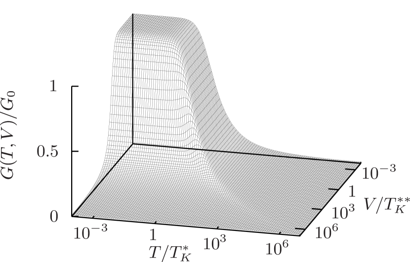
Figure 2: The differential conductance $G(T,V)$ as function of temperature and voltage, scaled by the unitary conductance $G_{0}=G(T=V=0)=2e^{2}/h$. All RG equations were considered in third order truncation and solved numerically.

The temperature and voltage are scaled by $T_{K}^{*}$ and $T_{K}^{**}$, respectively, as defined by Eqs. (3) and (10). The plateau in the upper left corner of Fig. 2 corresponds to the unitary conductance $G_{0}=\frac{2e^{2}}{h}$ which is reached if both temperature and voltage are several orders of magnitude smaller than the Kondo temperature.

Figure 3: (Color online) The differential conductance $G_{V}(T)$ as function of temperature for constant voltage. The solid (dashed) lines show the results of the calculations in third (second) order truncation.

Figure 3 shows the $T$-dependence of the differential conductance for six different fixed values of $V$. For $V=0$, the temperature dependence of the conductance has already been compared to numerically exact NRG calculations in Ref. pletyukhov_hs_PRL12, , where a deviation $\lesssim 3\%$ has been found in the whole temperature regime independent of the truncation order. For finite voltage, the results for the second and third order truncation schemes agree quite well if the temperature and the voltage are scaled by the corresponding values of $T_{K}^{*}$ and $T_{K}^{**}$, respectively. In the range

$$10^{-4}\leq\frac{T}{T_{K}^{*}},\frac{V}{T_{K}^{**}}\leq 10^{7},$$ (430)

which is plotted in Fig. 2, the maximal deviation in the differential conductance $G(T,V)$ between both truncation schemes is less than $15\%$. In contrast, the ratio $\frac{T_{K}^{*}}{T_{K}^{**}}$ depends crucially on the truncation order, which seems to hold also for other ratios of low-energy scales within our method when applied to the strong coupling regime (see the next section). We obtain $\frac{T_{K}^{*}}{T_{K}^{**}}\approx 1.044$ in second order truncation, and

$$\frac{T_{K}^{*}}{T_{K}^{**}}\approx 0.623$$ (431)

in third order truncation. Since the result in third order truncation is expected to lie closer to the correct result (see also the next section), the last result may serve as a guideline for more precise calculations in the future. We note that our prediction is quite close to the result $T_{K}^{*}/T_{K}^{**}\sim 0.66$ obtained in Ref. spataru_PRB10, , where the $GW$ approximation within the $\sigma G\sigma W$ formalism has been used for the symmetric Anderson model. Taking our result, the Fermi liquid coefficients $c_{T}^{**}$ and $c_{V}^{**}$ can be calculated from Eqs. (7) and (12), leading to the prediction

$$c_{T}^{**}\approx 16.95,\quad c_{V}^{**}\approx 2.58.$$ (432)

Figure 3 clearly shows that the differential conductance $G_{V}(T)\equiv G(T,V)$ is in general not a monotonous function of $T$ if $V$ is fixed.

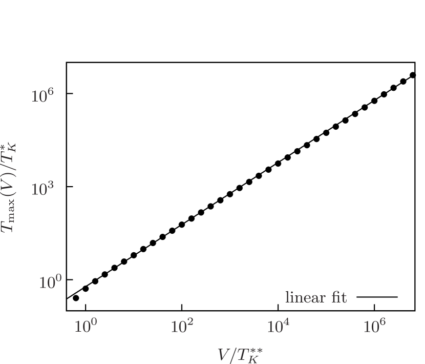
Figure 4: The position $T_{\text{max}}$ of the peak in the differential conductance $G_{V}(T)$, calculated within the third order truncation scheme, at constant voltage $V$, cf. the solid lines in Fig. 3. The solid line corresponds to the linear fit $\frac{T}{T_{K}^{*}}=0.597653\frac{V}{T_{K}^{**}}$ at large voltages.

Figure 5: The position $T_{\text{max}}$ of the peak in the differential conductance $G_{V}(T)$, calculated within the second order truncation scheme, at constant voltage $V$, cf. the dashed lines in Fig. 3. The solid line corresponds to the linear fit $\frac{T}{T_{K}^{*}}=0.399717\frac{V}{T_{K}^{**}}$ at large voltages.

For $V\gtrsim T_{K}^{**}$, there is a pronounced maximum. Figure 4 shows how the position $T_{\text{max}}(V)$ of this maximum depends on the voltage $V$ (if the RG equations are solved using the third order truncation). For $V\gtrsim T_{K}^{*}$, i.e., in the regime where there is a pronounced maximum, the function $T_{\max}(V)$ can be approximated quite well by a linear fit over six orders of magnitude in the ratio $V/T_{K}^{**}$. Figure 5 shows that the behavior is very similar if the conductance is calculated within the second order truncation scheme.

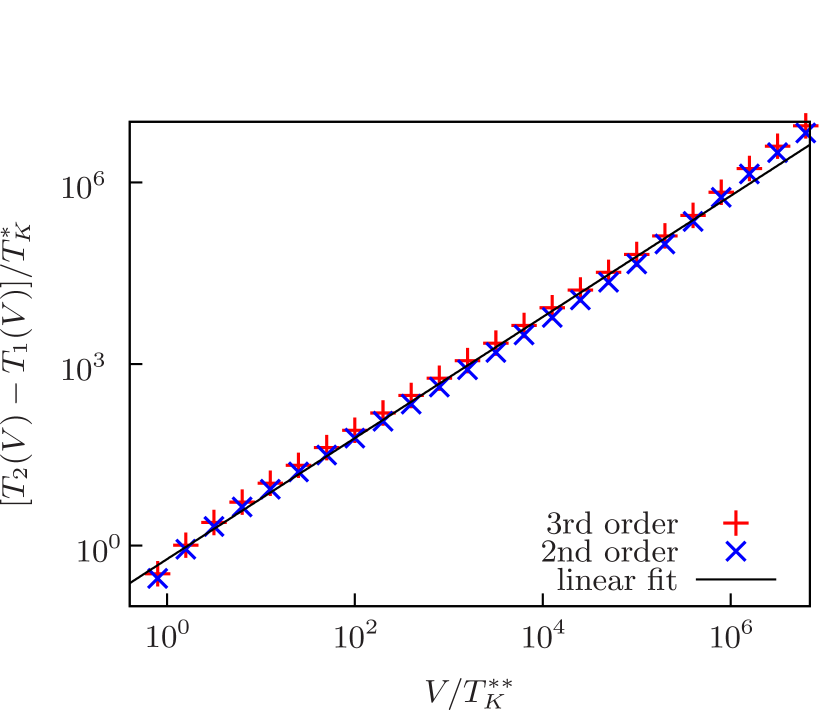
Figure 6: (Color online) The width $T_{2}(V)-T_{1}(V)$ of the peak in the differential conductance $G_{V}(T)$ at finite voltage $V$, cf. Fig. 3. $T_{1}(V)$ and $T_{2}(V)$ are the temperatures for which $G_{V}[T_{i}(V)]-G_{V}(T=0)=\frac{1}{2}[G_{V}(T=0)+G_{V}(T_{\text{max}}(V))]$, $i=1,2$. The solid line corresponds to the linear fit $\frac{T}{T_{K}^{*}}=0.597653\frac{V}{T_{K}^{**}}$ that has been used in Fig. 4.

This linear fit from Fig. 4 appears to be a reasonable approximation also for the width of the peak of the function $G_{V}(T)$ at fixed $V$, see Fig. 6. We define the peak width as the difference $T_{2}(V)-T_{1}(V)$, where $T_{i}(V)$, $i=1,2$, are chosen such that $G_{V}[T_{i}(V)]$ is the average of the zero-temperature conductance $G_{V}(T=0)$ and the maximum value $G_{V}[T_{\text{max}}(V)]$. This means that the excess conductance $G_{V}(T)-G_{V}(T=0)$ reaches exactly half its maximum value at $T_{i}(V)$, $i=1,2$.

At first sight, it might seem counter-intuitive that the conductance can increase for increasing temperature since temperature acts as a cutoff of the RG-flow, as can be seen from the form of the integrals in Eqs. (279)-(283). However, by looking at the final RG equations (347)-(353), one can see that the cutoff provided by the voltage $V$ is very different and by no means an overall cutoff for all quantities. In particular, the quantities for $E=i\Lambda$ and for $E=\pm V+i\Lambda$ have a considerably different flow as function of $\Lambda$ and are coupled to each other in a complicated way. For finite $V\gtrsim T_{K}^{**}$ and $T=0$, this leads to the effect that the conductance shows a maximum for $E=i\Lambda\sim iT_{K}^{**}$ as function of the flow parameter $\Lambda$. This in turn leads to a maximum for the temperature dependence of the conductance since temperature is an overall cutoff for all quantities. Besides this subtle technical explanation, a more physical interpretation can be given in terms of the spectral function of the Kondo model, which is believed to have side-peaks at $\omega\sim\pm V$.Meir_etal_PRL93 ; Koenig_etal_PRL96 Therefore, when temperature is of the order of the voltage, these side peaks can be reached and give rise to an enhanced conductance.

VI.2 Expansion of the differential conductance for small temperature and/or voltage

We now consider temperatures and voltages much smaller than the Kondo temperature and calculate numerical approximations for the coefficients $c_{T}^{*}$ and $c_{V}^{*}$, which appear in the Fermi liquid result (6), using the differential conductance obtained in the second and third order truncation schemes. We note again that due to our improved scheme for determining the initial condition of the RG flow at finite voltage (see Section V.9), we obtain here an improved result for the Fermi liquid coefficient $c_{V}^{*}$ in comparison to Ref. pletyukhov_hs_PRL12, . Our result for the coefficient $c_{T}^{*}$ is the same as in Ref. pletyukhov_hs_PRL12, , but since recent NRG calculations merker_PRB13 have obtained an improved value for $c_{T}^{*}$, the quality of our results has to be revisited also for this quantity.

Figures 7 and 8 visualize how the coefficients $c_{T}^{*}$ and $c_{V}^{*}$ can be determined in second and third order, respectively, using a suitable plot of the differential conductance.

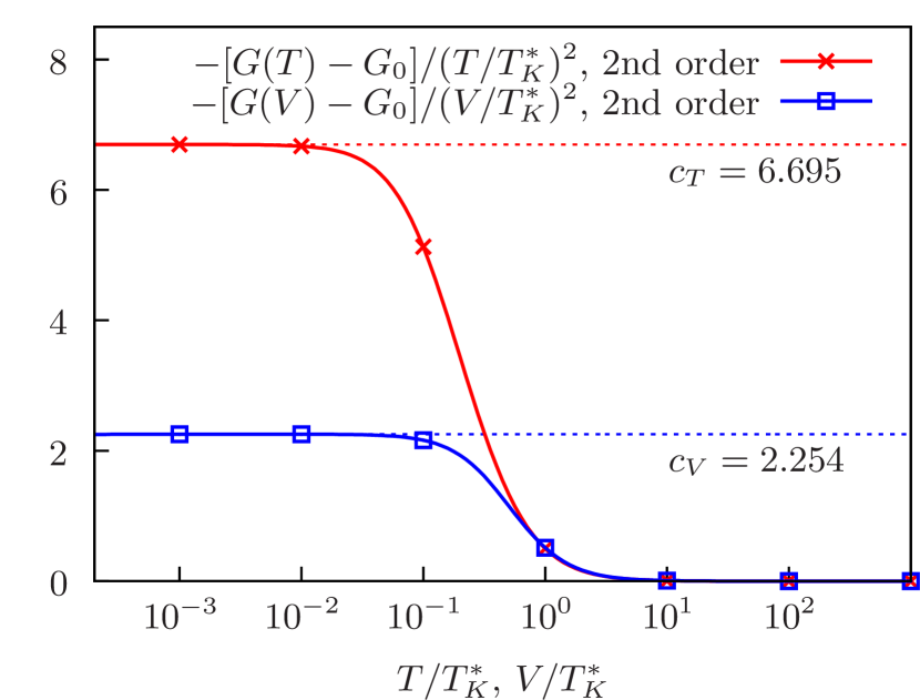
Figure 7: (Color online) Quadratic fit for the differential conductance $G(T)\equiv G_{V=0}(T)$ in second order truncation at low temperatures and $G(V)\equiv G_{T=0}(V)$ at low voltages, respectively. The differential conductance is plotted in such a way that the coefficients $c_{T}^{*}$ and $c_{V}^{*}$ in the expansions $G(T)/G_{0}\approx 1-c_{T}^{*}\left(\frac{T}{T_{K}^{*}}\right)^{2}$ and $G(V)/G_{0}\approx 1-c_{V}^{*}\left(\frac{V}{T_{K}^{*}}\right)^{2}$ can be identified easily.

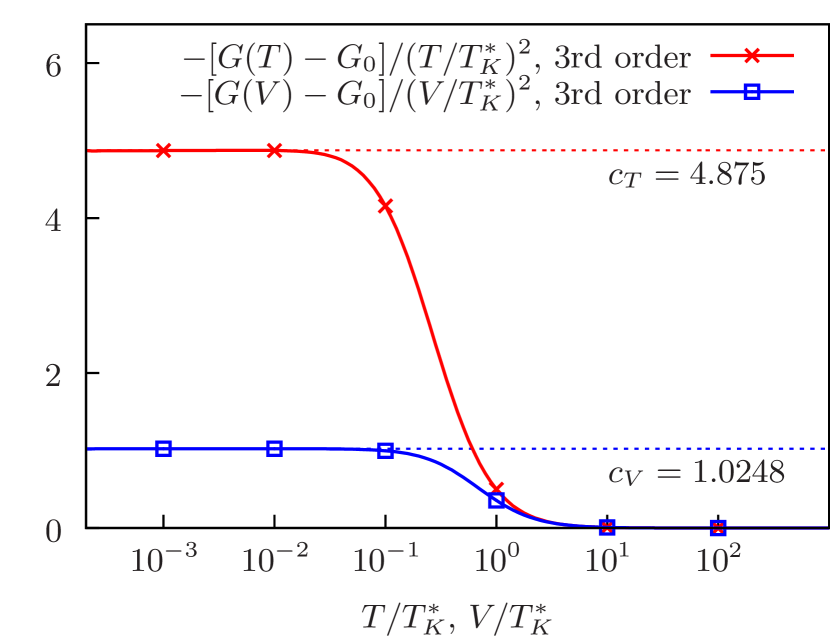
Figure 8: (Color online) Quadratic fit for the differential conductance $G(T)\equiv G_{V=0}(T)$ in third order truncation at low temperatures and $G(V)\equiv G_{T=0}(V)$ at low voltages, respctively, cf. Fig. 7.

When comparing the results in second and third order to the known results (5) and (7), it is important to note that the Fermi liquid coefficients are ratios of various low-energy scales in different energy regimes

$$c_{T}^{*}=\left(\frac{T_{K}^{*}}{T_{K}^{\prime}}\right)^{2},\quad c_{V}^{*}=\left(\frac{T_{K}^{*}}{T_{K}^{\prime\prime}}\right)^{2},$$ (433)

where the scales $T_{K}^{\prime},T_{K}^{\prime\prime}$ characterize the curvature of the function $H(T,V)=1-G(T,V)/G_{0}$ w.r.t. temperature and voltage at $T=V=0$,

$$\left(\frac{1}{T_{K}^{\prime}}\right)^{2}=\frac{1}{2}\frac{\partial^{2}H}{\partial T^{2}}\bigg{|}_{T=V=0},\quad\left(\frac{1}{T_{K}^{\prime\prime}}\right)^{2}=\frac{1}{2}\frac{\partial^{2}H}{\partial V^{2}}\bigg{|}_{T=V=0}.$$ (434)

Analogously, one can write the Fermi liquid coefficients $c_{T}^{**}$ and $c_{V}^{**}$, defined by Eq. (6), as

$$c_{T}^{**}=\left(\frac{T_{K}^{**}}{T_{K}^{\prime}}\right)^{2},\quad c_{V}^{**}=\left(\frac{T_{K}^{**}}{T_{K}^{\prime\prime}}\right)^{2}.$$ (435)

As a consequence, the absolute values of the Fermi liquid coefficients relate energy scales close to $T_{K}$ (represented by $T_{K}^{*}$ or $T_{K}^{**}$) to energy scales very far below $T_{K}$ (represented by $T_{K}^{\prime}$ or $T_{K}^{\prime\prime}$), i.e. they probe the correlation between different energy regimes. In contrast, the ratio of the Fermi liquid coefficients

$$\frac{c_{V}}{c_{T}}=\frac{c_{V}^{*}}{c_{T}^{*}}=\frac{c_{V}^{**}}{c_{T}^{**}}=\left(\frac{T_{K}^{\prime}}{T_{K}^{\prime\prime}}\right)^{2}$$ (436)

probes only the energy regime very far below the Kondo temperature, analog to the ratio $\frac{T_{K}^{*}}{T_{K}^{**}}$, which probes only the energy regime close to $T_{K}$.

Since only the ratios of the various energy scales $T_{K}^{*},T_{K}^{**},T_{K}^{\prime}$ and $T_{K}^{\prime\prime}$ are universal, conclusions about the reliability of the method are not unambigious when comparing the known results (5) and (7)

$$\sqrt{c_{T}^{*}} =\frac{T_{K}^{*}}{T_{K}^{\prime}}\approx 2.57,\quad\sqrt{c_{V}^{*}}=\frac{T_{K}^{*}}{T_{K}^{\prime\prime}}\approx 1.00,$$ (437)

$$\sqrt{\frac{c_{V}^{*}}{c_{T}^{*}}} =\frac{T_{K}^{\prime}}{T_{K}^{\prime\prime}}=\frac{\sqrt{3}}{\pi\sqrt{2}}\approx 0.39$$ (438)

to the results in second order truncation

$$\frac{T_{K}^{*}}{T_{K}^{\prime}} \approx 2.59,\quad\frac{T_{K}^{*}}{T_{K}^{\prime\prime}}\approx 1.5,\quad\frac{T_{K}^{\prime}}{T_{K}^{\prime\prime}}\approx 0.58,$$ (439)

or to the ones in third order truncation

$$\frac{T_{K}^{*}}{T_{K}^{\prime}} \approx 2.21,\quad\frac{T_{K}^{*}}{T_{K}^{\prime\prime}}\approx 1.01,\quad\frac{T_{K}^{\prime}}{T_{K}^{\prime\prime}}\approx 0.46.$$ (440)

The fact that $\frac{T_{K}^{*}}{T_{K}^{\prime}}$ is quite close to the correct result in second order truncation, whereas $\frac{T_{K}^{*}}{T_{K}^{\prime\prime}}$ is very precise in third order truncation, might be an accident since the ratio of two energy scales can have a significantly different error than the energy scales themselves. Overall we observe that all ratios depend significantly on the truncation order and, if the ratio of two energy scales from the same energy regime is taken, the result improves when increasing the truncation order. For example, the ratio $\frac{T_{K}^{\prime}}{T_{K}^{\prime\prime}}$ improves from $49\%$ deviation in second order to $18\%$ error in third order truncation. Furthermore, we expect that a perturbative truncation of the RG equations should lead to a better improvement for larger energy scales when increasing the truncation order. Therefore, we speculate that our result (431) for $\frac{T_{K}^{*}}{T_{K}^{**}}$ in third order truncation might have an even better quality than the corresponding result for the ratio $\frac{T_{K}^{\prime}}{T_{K}^{\prime\prime}}$. This is also in accordance with the fact that the result (9) is in agreement with experiment and in agreement with another recent effective action method smirnov_grifoni_PRB03 . Moreover, as already mentioned in Sec. VI.1, our result (431) for the ratio $T_{K}^{*}/T_{K}^{**}$ is very close to the result of Ref. spataru_PRB10, . This provides evidence that our results in third order truncation are quite reliable for temperatures and voltages close to the Kondo temperature. Furthermore, speculating that $T_{K}^{*}$ and $T_{K}^{**}$ are approximately correct in third order truncation, the precise result for $\frac{T_{K}^{*}}{T_{K}^{\prime\prime}}$ in the same order indicates that $T_{K}^{\prime\prime}$ is quite reliable, i.e. it seems that the voltage dependence can also be trusted for small voltages $V\ll T_{K}$. In contrast, the poor result for $\frac{T_{K}^{*}}{T_{K}^{\prime}}$ in third order truncation indicates that $T_{K}^{\prime}$ deviates significantly from the correct result, i.e. the temperature dependence is not so well described for $T\ll T_{K}$. Therefore, it seems that the rather precise result for $\frac{T_{K}^{*}}{T_{K}^{\prime}}$ in second order truncation is an accident and originates from the fact that both $T_{K}^{*}$ and $T_{K}^{\prime}$ are incorrect by approximately the same factor, whereas, in third order truncation, $T_{K}^{*}$ is more precise than $T_{K}^{\prime}$, leading to the counterintuitive effect that the quality of $\frac{T_{K}^{*}}{T_{K}^{\prime}}$ decreases with increasing truncation order.

In summary, we have presented arguments that the voltage dependence of the conductance seems to be quite reliable in third order truncation, whereas the temperature dependence needs to be improved in the regime $T\ll T_{K}$. Nevertheless, our arguments are partially based on speculations and need further substantiation by improved calculations for the nonequilibrium Kondo model in the strong coupling regime. Furthermore, we note that the third order RG scheme is in principle capable of reproducing the Fermi liquid result $\frac{c_{V}}{c_{T}}=\frac{3}{2\pi^{2}}$ exactly when an analytical solution of the RG equations is done for either $V=0$ and $T\ll T_{K}$ or $T=0$ and $V\ll T_{K}$, and $\frac{c_{V}}{c_{T}}$ is expanded systematically in orders of $J$, see Ref. pletyukhov_hs_PRL12, for details. The numerical solution contains all terms up to a certain order in $J$, but higher order terms which are not treated consistently cause deviations from the exact value for $\frac{c_{V}}{c_{T}}$.

We note that our improved scheme to determine $c_{V}^{*}$ can also be applied to the $S=1$ Kondo model and to the calculation of the Fermi liquid coefficients of the static magnetic susceptibility $\chi/\chi_{0}=1-a_{T}(T/T_{K})^{2}-a_{V}(V/T_{K})^{2}$, where the authors of Ref. hoerig_mora_schuricht_PRB14, report the following changes to their results in third order truncation hoerig_privat

$$\left.\frac{c_{V}}{c_{T}}\right|_{S=1} =0.179,$$ (441)

$$\left.\frac{a_{V}}{a_{T}}\right|_{S=1/2} =0.11, \left.\frac{a_{V}}{a_{T}}\right|_{S=1} =0.10.$$ (442)

For $S=1$, their results for $\frac{c_{V}}{c_{T}}$ deviate by $\sim 9\%$ from the exact value $\frac{c_{V}}{c_{T}}=\frac{3}{2\pi^{2}}\frac{4+10S}{5+8S}\approx 0.164$, as derived in Ref. hoerig_mora_schuricht_PRB14, .

VI.3 Comparison with experiments

We have compared our calculations with experimental results obtained by Kretinin et al.kretinin_PRB85 They measured the differential conductance at finite temperature and voltage in an InAs nanowire-based quantum dot. This system can be described by the Kondo model, provided that both temperature and voltage are sufficiently small to suppress charge fluctuations. In previous publications, only the results for $G(T=0,V)$ and $G(T,V=0)$ have been compared between theory and experiment, here we present the comparison where both temperature and bias voltage are finite.

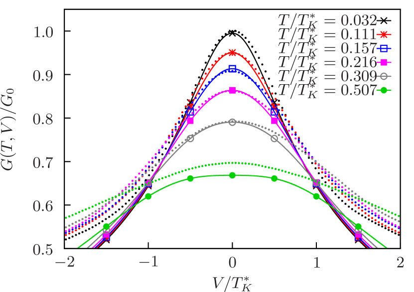
Figure 9: (Color online) Comparison of the differential conductance $G_{T}(V)$ for fixed $T$ calculated with RTRG (solid lines) with experimental data from Ref. kretinin_PRB85, (dots).

Figure 10: (Color online) Comparison of the differential conductance $G_{V}(T)$ for fixed $V$ calculated with RTRG (solid lines) with experimental data from Ref. kretinin_PRB85, (dots).

In Figs. 9 and 10, either the temperature or the voltage is fixed, and the differential conductance $G$ is plotted as function of the other quantity. Both figures compare the results for six different fixed values of the temperature or the voltage, respectively.

We find good agreement between our calculations and the experiment if temperature and voltage are much smaller than the Kondo temperature. If either of these quantities is too large, charge fluctuations become important, which cannot be described properly by the Kondo model that our calculations are based on.

In an earlier publication,klochan_scaling_kondo_ZBP results obtained with the method presented here had been used to determine the Kondo temperature of an experimental device and the temperature at which the experiment had been performed.

VII Summary and outlook

In this paper, we presented a real time renormalization group approach that extends the flow scheme introduced in Ref. pletyukhov_hs_PRL12, , which uses the Fourier variable as the flow parameter. We showed how universal RG equations can be set up in all orders and that only an expansion in the frequency-independent effective two-point vertex is needed to guarantee convergence of all frequency integrals. The RG equations can be solved in various truncation orders providing a consistency check for the reliability of the results. Whereas in this paper the RG equations have been solved explicitly up to third order truncation for the Kondo model, we have also outlined the procedure how to determine all terms in fourth order truncation. This might be helpful for future applications to test the reliability of the results even further.

We have shown that universality can be achieved for the Kondo model by using appropriate boundary conditions including the universal stationary conductance at zero temperature and zero bias voltage. With our procedure it is possible to arrive at stable results already for initial cutoffs which are about six orders of magnitude larger than the Kondo temperature. This is a significant improvement compared to other methods trying to solve directly for the universal properties of the Kondo model instead of the more involved Anderson impurity model.

We applied the method to the nonequilibrium spin-$\frac{1}{2}$ Kondo model at zero magnetic field but arbitrary temperature and voltage. We found that the temperature-dependent conductance $G_{V}(T)$ at fixed voltage $V$ exhibits non-monotonic behavior. The height and width of the appearing local peak were shown to scale linearly with the applied voltage over approximately six orders of magnitude in units of the Kondo temperature. We compared our results to recent experiments and found good agreement in the regime where the Kondo model is expected to describe the experimental system accurately.

To characterize the temperature and voltage dependence of the conductance in different energy regimes close and far below the Kondo temperature, we have defined four different energy scales $T_{K}^{*}$, $T_{K}^{**}$, $T_{K}^{\prime}$, and $T_{K}^{\prime\prime}$. The scales $T_{K}^{\prime}$/$T_{K}^{\prime\prime}$ are defined from the curvature of $G_{V=0}(T)$/$G_{T=0}(V)$ at $T=0$/$V=0$, and the scales $T_{K}^{*}$/$T_{K}^{**}$ by the half width at half maximum of the peak of $G_{V=0}(T)$/$G_{T=0}(V)$ at $T=0$/$V=0$. All these energy scales are proportional to the Kondo temperature $T_{K}$. We found that the shape of the conductance $G(T,V)$ is independent of the truncation order when $T$ and $V$ are scaled in units of $T_{K}^{*}$ and $T_{K}^{**}$, respectively, providing evidence for the reliability of our result for the temperature and voltage dependence of the conductance. However, an interesting issue is the determination of the three independent universal ratios of the four characteristic energy scales, which turn out to depend crucially on the truncation order. The ratio $\frac{T_{K}^{\prime}}{T_{K}^{\prime\prime}}=\frac{\sqrt{3}}{\pi\sqrt{2}}\approx 0.39$ is known exactly from Fermi liquid relations, relating the temperature and voltage dependence for $T,V\ll T_{K}$. Numerically exact results exist for the ratio $\frac{T_{K}^{*}}{T_{K}^{\prime}}\approx 2.57$ from recent NRG calculations, relating the temperature dependence for $T\sim T_{K}$ to the one for $T\ll T_{K}$. Our method predicts in third order truncation the result $\frac{T_{K}^{*}}{T_{K}^{**}}\approx 0.62$ for the remaining unknown ratio, relating the temperature and voltage dependence at energies close to $T_{K}$. We presented evidence for the reliability of this result in third order approximation, based on the result $G_{T=0}(V=T_{K}^{*})\approx\frac{2}{3}G_{0}$, which has been confirmed experimentally and by another recent effective action method. From a comparison of our results for the other two ratios in third order truncation with the exact ones we obtained evidence that our results for the voltage dependence of the conductance are quite accurate for all voltages, whereas the ones for the temperature dependence need to be improved for $T\ll T_{K}$.

Concerning future directions, the $E$-flow scheme offers a systematic method to avoid $\frac{1}{E^{n}}$ and logarithmic divergencies by resumming self-energy insertions and vertex corrections. Since approximation schemes in different truncation orders can be defined, its reliability can be tested by itself, in particular in those regimes where the vertices start to grow. So far, applications were successful for $2$-level models where the dynamics of the local system is driven by spin fluctuations (Kondo model), energy fluctuations (spin-boson model) or charge fluctuations (interacting resonant level model). In the future, it is of particular interest to understand the interplay between these fluctuations, as described, e.g., by the Anderson impurity model (spin and charge fluctuations) or by quantum dots coupled to a bosonic environment (charge/spin and energy fluctuations). In particular, the Anderson impurity model is expected to be a suitable model to extract the universal behavior in the Kondo regime without resorting to the boundary condition of universal conductance, as used in this paper. This is motivated by recent NRG studies,hanl_PRB14 where it was shown that universality is reached much faster for the Anderson impurity model compared to the Kondo model. Furthermore, the Anderson impurity model allows for the study of potential scattering terms away from the particle-hole symmetric point and logarithmic energy renormalizations in the mixed-valence regime. Other interesting applications for the $E$-flow scheme are generic $n$-level quantum dots and models with quantum critical behavior, like, e.g., the sub-Ohmic spin-boson model or multi-channel Kondo models.

Appendix A Evaluation of the integrals in the $E$-flow equations for the isotropic Kondo model

We will now discuss how the integrals (279)–(283), which occur in the $E$-flow RG equations for the Kondo model, can be evaluated:

$$F^{(1)}_{12} =Z_{12}\int d\omega\int d\omega^{\prime}\frac{f^{\prime}(\omega)f^{\prime}(\omega^{\prime})}{\omega+\omega^{\prime}+\chi_{12}},$$ (443)

$$F^{(1)}_{12,34} =Z_{12}Z_{34}$$

$$\ \int d\omega\int d\omega^{\prime}\frac{f^{\prime}(\omega)f^{a}(\omega^{\prime})}{(\omega+\omega^{\prime}+\chi_{12})(\omega+\omega^{\prime}+\chi_{34})},$$ (444)

$$F^{(2)}_{12,34} =Z_{12}\int d\omega\int d\omega^{\prime}\frac{{\mathcal{F}}_{34}(\omega)f^{\prime}(\omega)f^{\prime}(\omega^{\prime})}{\omega+\omega^{\prime}+\chi_{12}},$$ (445)

$$F^{(3)}_{12} =-Z_{12}\int d\omega\frac{f^{\prime}(\omega)}{\omega+\chi_{12}},$$ (446)

$$F^{(4)}_{12,34} =Z_{12}\int d\omega\frac{{\mathcal{F}}_{34}(\omega)f^{\prime}(\omega)}{\omega+\chi_{12}},$$ (447)

where the integral $\mathcal{F}_{12}(\omega)=\mathcal{F}\left(E_{12},\omega\right)$ is given by Eq. (119),

$$\mathcal{F}_{12}(\omega) =Z_{12}\int d\omega^{\prime}f^{a}\left(\omega^{\prime}\right)$$ (448)

$$\quad\quad\quad\quad\left[\frac{1}{\omega+\omega^{\prime}+\chi_{12}}-\frac{1}{\omega^{\prime}+\chi_{12}}\right].$$

We note that $\mathcal{F}_{12}(0)=0$.

A.1 Integrals at zero temperature

For $T=0$, we can use

$$f(\omega) =1-\Theta(\omega)\quad\Rightarrow\quad f^{\prime}(\omega)=-\delta(\omega)$$ (449)

to evaluate the integrals and get

$$F^{(1)}_{12} =\frac{Z_{12}}{\chi_{12}}=\frac{1}{E_{12}+i\Gamma\left(E_{12}\right)},$$ (450)

$$F^{(1)}_{12,34} =\begin{cases}\frac{Z_{12}^{2}}{\chi_{12}}=Z_{12}F^{(1)}_{12}&\text{if $E_{12}=E_{34}$,}\\ \frac{Z_{12}Z_{34}}{\chi_{12}-\chi_{34}}(\ln{\chi_{12}}-\ln{\chi_{34}})&\text{otherwise,}\end{cases}$$ (451)

$$F^{(2)}_{12,34} =Z_{12}\frac{\mathcal{F}_{34}(0)}{\chi_{12}}=0,$$ (452)

$$F^{(3)}_{12} =\frac{Z_{12}}{\chi_{12}}=\frac{1}{E_{12}+i\Gamma\left(E_{12}\right)},$$ (453)

$$F^{(4)}_{12,34} =-Z_{12}\frac{\mathcal{F}_{34}(0)}{\chi_{12}}=0.$$ (454)

In the special case that no bias voltage is applied, i.e., all chemical potentials are the same, and

$$E_{12} =E, Z_{12} =Z, \chi_{12} =\chi,$$ (455)

the integrals are

$$F^{(1)}_{12} =\frac{1}{E+i\Gamma\left(E\right)},$$ (456)

$$F^{(1)}_{12,34} =\frac{Z}{E+i\Gamma\left(E\right)},$$ (457)

$$F^{(2)}_{12,34} =0,$$ (458)

$$F^{(3)}_{12} =\frac{1}{E+i\Gamma\left(E\right)},$$ (459)

$$F^{(4)}_{12,34} =0.$$ (460)

A.2 Integrals at finite temperature

A.2.1 Prerequisites

For finite $T$, the Fermi function, its antisymmetric part, and its derivative are

$$f(\omega) =\frac{1}{2}-T\sum_{n\in\mathbb{Z}}\frac{1}{\omega-i\omega_{n}},$$ (461)

$$f^{a}(\omega) =\phantom{\frac{1}{2}}-T\sum_{n\in\mathbb{Z}}\frac{1}{\omega-i\omega_{n}},$$ (462)

$$f^{\prime}(\omega) =\phantom{\frac{1}{2}-}T\sum_{n\in\mathbb{Z}}\frac{1}{(\omega-i\omega_{n})^{2}},$$ (463)

where

$$\omega_{n}=2\pi T\left(n+\frac{1}{2}\right)$$ (464)

is a Matsubara frequency for any integer number $n$. The integrals are calculated by closing the integration path in the upper half of the complex plane and applying the residue theorem. Note that $\chi_{ij}$ is an analytic function in the upper half of the complex plane, such that the only poles in the upper half plane are the poles of the Fermi function or its derivative, which are first and second order poles, respectively.

In the following, we will often use the shorthand notations

$$Z =Z_{12},$$ (465)

$$\bar{Z} =Z_{34},$$ (466)

$$\gamma =\frac{\chi_{12}}{2\pi iT},$$ (467)

$$\bar{\gamma} =\frac{\chi_{34}}{2\pi iT}.$$ (468)

A.2.2 Polygamma Functions

The polygamma functions are derivatives of the logarithm of the Gamma function $\Gamma(z)$. They can be used to evaluate series of resolvents that contain Matsubara frequencies. The first polygamma function, also called digamma function, is given by

$$\psi(z) =\frac{d}{dz}\ln\Gamma(z)=-\widehat{\gamma}+\sum_{n=0}^{\infty}\left(\frac{1}{n+1}-\frac{1}{n+z}\right),$$ (469)

where $\widehat{\gamma}$ is the Euler-Mascheroni constant. The digamma function permits us to evaluate series of the form

$$\sum_{n=0}^{\infty}\left(\frac{1}{n+z_{1}}-\frac{1}{n+z_{2}}\right)=\psi(z_{2})-\psi(z_{1}).$$ (470)

Further types of series can be evaluated using the derivatives of the digamma function,

$$\psi^{\prime}(z) =\phantom{-}\sum_{n=0}^{\infty}\frac{1}{(n+z)^{2}},$$ (471)

$$\psi^{\prime\prime}(z) =-\sum_{n=0}^{\infty}\frac{2}{(n+z)^{3}}.$$ (472)

A.2.3 Integrals which depend only on $E_{12}$

For the integral $F^{(1)}_{12}$, we get

$$F^{(1)}_{12} =Z\int d\omega\int d\omega^{\prime}\frac{f^{\prime}(\omega)f^{\prime}(\omega^{\prime})}{\omega+\omega^{\prime}+\chi}$$

$$=Z\,T^{2}\sum_{n\in\mathbb{Z}}\sum_{m\in\mathbb{Z}}\int d\omega\int d\omega^{\prime}$$

$$\quad\quad\quad\quad\quad\frac{1}{(\omega-i\omega_{n})^{2}}\frac{1}{(\omega^{\prime}-i\omega_{m})^{2}}\frac{1}{\omega+\omega^{\prime}+\chi}$$

$$=Z\,(2\pi iT)T\sum_{n=0}^{\infty}\sum_{m\in\mathbb{Z}}\int d\omega^{\prime}\frac{1}{(\omega^{\prime}-i\omega_{m})^{2}}$$

$$\quad\quad\quad\quad\quad\times\frac{-1}{(i\omega_{n}+\omega^{\prime}+\chi)^{2}}$$

$$=Z\,(2\pi iT)^{2}\sum_{n=0}^{\infty}\sum_{m=0}^{\infty}\frac{2}{(i\omega_{n}+i\omega_{m}+\chi)^{3}}.$$ (473)

Using $i\omega_{n}=2\pi iT\left(n+\frac{1}{2}\right)$ and $\chi=(2\pi iT)\gamma$, this yields

$$F^{(1)}_{12} =\frac{Z}{2\pi iT}\sum_{n=0}^{\infty}\sum_{m=0}^{\infty}\frac{2}{(n+m+\gamma+1)^{3}}$$

$$\overset{N=n+m}{=}2\frac{Z}{2\pi iT}\sum_{N=0}^{\infty}\sum_{m=0}^{N}\frac{1}{(N+\gamma+1)^{3}}.$$ (474)

Note that there are $N+1$ equal terms in the $m$-sum:

$$F^{(1)}_{12} =2\frac{Z}{2\pi iT}\sum_{N=0}^{\infty}\frac{N+1}{(N+\gamma+1)^{3}}$$

$$=2\frac{Z}{2\pi iT}\sum_{N=0}^{\infty}\frac{N+\gamma+1-\gamma}{(N+\gamma+1)^{3}}$$

$$=2\frac{Z}{2\pi iT}\sum_{N=0}^{\infty}\left[\frac{1}{(N+\gamma+1)^{2}}-\gamma\frac{1}{(N+\gamma+1)^{3}}\right]$$

$$=\frac{Z}{2\pi iT}\left[2\psi^{\prime}(\gamma+1)+\gamma\psi^{\prime\prime}(\gamma+1)\right].$$ (475)

Evaluating the integral $F^{(3)}_{12}$ yields

$$F^{(3)}_{12} =-Z\int d\omega\frac{f^{\prime}(\omega)}{\omega+\chi}$$

$$=-Z\,T\sum_{n\in\mathbb{Z}}\int d\omega\frac{1}{(\omega-i\omega_{n})^{2}}\frac{1}{\omega+\chi}$$

$$=Z(2\pi iT)\sum_{n=0}^{\infty}\frac{1}{(i\omega_{n}+\chi)^{2}}$$

$$=\frac{Z}{2\pi iT}\sum_{n=0}^{\infty}\frac{1}{\left(n+\gamma+\frac{1}{2}\right)^{2}}$$

$$=\frac{Z}{2\pi iT}\psi^{\prime}\left(\gamma+\frac{1}{2}\right).$$ (476)

A.2.4 Integrals which depend on $E_{12}$ and $E_{34}$

The evaluation of the integrals that depend on two $E$-arguments can be done analogously. The calculations are straightforward, but lengthy. Therefore, we only list the results here.

In the special case that both $E$-arguments are equal, we get

$$F^{(1)}_{12,12} =Z\,F^{(1)}_{12},$$ (477)

$$F^{(2)}_{12,12} =\frac{Z^{2}}{2\pi iT}\left\{\left[2\psi^{\prime}(\gamma+1)+\gamma\psi^{\prime\prime}(\gamma+1)\right]\left[\psi(\gamma+1)-\psi\left(\gamma+\frac{1}{2}\right)-1\right]+\gamma\left[\psi^{\prime}(\gamma+1)\right]^{2}-\frac{1}{2}\psi^{\prime\prime}(\gamma+1)\right\},$$ (478)

$$F^{(4)}_{12,12} =\frac{Z^{2}}{2\pi iT}\left\{\psi^{\prime}\left(\gamma+\frac{1}{2}\right)\left[\psi\left(\gamma+\frac{1}{2}\right)-\frac{1}{2}\psi\left(\gamma+1\right)+1\right]-\psi^{\prime}(\gamma+1)\left[\frac{1}{2}\psi\left(\gamma+\frac{1}{2}\right)+1\right]\right.$$

$$\quad\quad\quad\quad\left.+\frac{1}{2}\sum_{k=0}^{\infty}\frac{d}{dk}\left[\frac{\psi(k+\gamma+1)}{k+\gamma+\frac{1}{2}}-\frac{\psi(k+\gamma+\frac{1}{2})}{k+\gamma+1}\right]\right\}.$$ (479)

If $E_{12}\neq E_{34}$, we get

$$F^{(1)}_{12,34} =\frac{Z\bar{Z}}{2\pi iT(\bar{\gamma}-\gamma)}\left[\psi(\bar{\gamma}+1)-\psi(\gamma+1)+\bar{\gamma}\psi^{\prime}(\bar{\gamma}+1)-\gamma\psi^{\prime}(\gamma+1)\right]$$ (480)

and

$$F^{(4)}_{12,34} =\frac{Z\bar{Z}}{2\pi iT}\left\{\psi^{\prime}\left(\gamma+\frac{1}{2}\right)\left[\psi\left(\bar{\gamma}+\frac{1}{2}\right)-\frac{1}{2}\psi\left(\bar{\gamma}+1\right)+\frac{1}{1-2(\bar{\gamma}-\gamma)}\right]\right.$$

$$\quad\quad-\psi^{\prime}(\bar{\gamma}+1)\left[\frac{1}{2}\psi\left(\gamma+\frac{1}{2}\right)+\frac{1}{1-2(\bar{\gamma}-\gamma)}\right]$$

$$\quad\quad\left.+\frac{1}{2}\sum_{k=0}^{\infty}\frac{d}{dk}\left[\frac{\psi(k+\bar{\gamma}+1)}{k+\gamma+\frac{1}{2}}-\frac{\psi(k+\gamma+\frac{1}{2})}{k+\bar{\gamma}+1}\right]\right\}.$$ (481)

No simple expression has been found for the integral $F^{(2)}_{12,34}$. We use the approximation

$$F^{(2)}_{12,34} \approx\frac{(Z_{12})^{2}F^{(2)}_{34,34}+(Z_{34})^{2}F^{(2)}_{12,12}}{2Z_{12}Z_{34}},$$ (482)

which, for $|E|\gg T,V$, neglects only contributions of $O(\frac{T,V}{|E|^{2}}J^{3})$ in the RG equations which are beyond subleading order, consistent with the strategy described in Section V.7.1. It has been verified that replacing the exact expressions for the integrals $F^{(1)}_{12,34}$ and $F^{(4)}_{12,34}$ by similar approximations only has a negligible effect on the results.

The approach used to evaluate the remaining series in $F^{(4)}_{12,34}$ is as follows:

• Sum the terms from $k=0$ to $k=k_{0}-1$ explicitly.

• Replace the remaining series, starting from $k=k_{0}$, by an integral.

We get

$$\sum_{k=k_{0}}^{\infty}\frac{d}{dk}\left[\frac{\psi(k+\bar{\gamma}+1)}{k+\gamma+\frac{1}{2}}-\frac{\psi(k+\gamma+\frac{1}{2})}{k+\bar{\gamma}+1}\right]$$

$$\approx \int_{k_{0}-\frac{1}{2}}^{\infty}\frac{d}{dk}\left[\frac{\psi(k+\bar{\gamma}+1)}{k+\gamma+\frac{1}{2}}-\frac{\psi(k+\gamma+\frac{1}{2})}{k+\bar{\gamma}+1}\right]$$ (483)

$$= -\left[\frac{\psi(k_{0}+\bar{\gamma}+\frac{1}{2})}{k_{0}+\gamma}-\frac{\psi(k_{0}+\gamma)}{k_{0}+\bar{\gamma}+\frac{1}{2}}\right].$$

The relative error caused by the approximation is

$$\epsilon \sim\frac{1}{4}\frac{1}{a^{2}}, a =\min\left\{\left|k_{0}+\bar{\gamma}+\frac{1}{2}\right|,|k_{0}+\gamma|\right\},$$ where (484)

and can be made arbitrarily small by choosing a suitable $k_{0}$.

Appendix B Subleading terms in the RG equations for the vertices in the Kondo model

B.1 Effective vertex $G_{12}(E)$

In the subleading terms in Eq. (303), different products of effective vertices occur, namely (without Fourier arguments and $F$-integrals)

$$\widehat{G}_{34}\widehat{G}_{12}\widehat{G}_{43}, \widehat{G}_{34}\widehat{G}_{13}\widehat{G}_{42}, \widehat{G}_{34}\widehat{G}_{42}\widehat{G}_{13},$$

$$\widehat{G}_{13}\widehat{G}_{42}\widehat{G}_{34}, \widehat{G}_{32}\widehat{G}_{14}\widehat{G}_{43},$$ (485)

which all have the form

$$\widehat{G}_{n_{1}n_{2}}\widehat{G}_{n_{3}n_{4}}\widehat{G}_{n_{5}n_{6}}\\ =\sum_{\chi\chi^{\prime}\chi^{\prime\prime}}G^{\chi}_{n_{1}n_{2}}G^{\chi^{\prime}}_{n_{3}n_{4}}G^{\chi^{\prime\prime}}_{n_{5}n_{6}}\widehat{L}^{\chi}_{n_{1}n_{2}}\widehat{L}^{\chi}_{n_{3}n_{4}}\widehat{L}^{\chi}_{n_{5}n_{6}},$$ (486)

where $n_{i}\in\{1,2,3,4\}$. Note that the $G^{\chi}_{n_{1}n_{2}}$ only depend on the reservoir indices, and the $\widehat{L}^{\chi}_{n_{1}n_{2}}$ only on the spin indices, and that we only consider $\chi,\chi^{\prime},\chi^{\prime\prime}\in\{2,3\}$, such that all occurring $\widehat{L}^{\chi}_{n_{1}n_{2}}$ contain the Pauli matrix $\underline{\sigma}_{n_{1}n_{2}}$:

$$\widehat{L}^{\chi}_{n_{1}n_{2}}\widehat{L}^{\chi^{\prime}}_{n_{3}n_{4}}\widehat{L}^{\chi^{\prime\prime}}_{n_{5}n_{6}}\\ =\sum_{i,j,k\in\{x,y,z\}}L^{\chi}_{i}L^{\chi^{\prime}}_{j}L^{\chi^{\prime\prime}}_{k}\sigma^{i}_{n_{1}n_{2}}\sigma^{j}_{n_{3}n_{4}}\sigma^{k}_{n_{5}n_{6}}.$$ (487)

To evaluate these subleading terms, we first evaluate the Pauli matrix products using the multiplication rule

$$\sigma^{i}_{13}\sigma^{j}_{32}=\delta_{ij}\delta_{12}+i\epsilon_{ijk}\sigma^{k}_{12}.$$ (488)

The results for the five different products in (485) are:

$$\sigma^{i}_{34}\sigma^{j}_{12}\sigma^{k}_{43} =2\delta_{ik}\sigma^{j}_{12},$$ (489)

$$\sigma^{i}_{34}\sigma^{j}_{13}\sigma^{k}_{42} =\left(\delta_{ij}\delta_{14}+i\epsilon_{jil}\sigma^{l}_{14}\right)\sigma^{k}_{42}$$

$$=\delta_{ij}\sigma^{k}_{12}+i\epsilon_{jik}\delta_{12}-\epsilon_{jil}\epsilon_{lkm}\sigma^{m}_{12}$$

$$=\delta_{ij}\sigma^{k}_{12}-i\epsilon_{ijk}\delta_{12}+\left(\delta_{ik}\delta_{jm}-\delta_{im}\delta_{jk}\right)\sigma^{m}_{12}$$

$$=\delta_{ij}\sigma^{k}_{12}+\delta_{ik}\sigma^{j}_{12}-\delta_{jk}\sigma^{i}_{12}-i\epsilon_{ijk}\delta_{12},$$ (490)

$$\sigma^{i}_{34}\sigma^{j}_{42}\sigma^{k}_{13} =\delta_{ij}\sigma^{k}_{12}+\delta_{ik}\sigma^{j}_{12}-\delta_{jk}\sigma^{i}_{12}+i\epsilon_{ijk}\delta_{12},$$ (491)

$$\sigma^{i}_{13}\sigma^{j}_{42}\sigma^{k}_{34} =\delta_{jk}\sigma^{i}_{12}+\delta_{ik}\sigma^{j}_{12}-\delta_{ij}\sigma^{k}_{12}-i\epsilon_{ijk}\delta_{12},$$ (492)

$$\sigma^{i}_{32}\sigma^{j}_{14}\sigma^{k}_{43} =\delta_{jk}\sigma^{i}_{12}+\delta_{ik}\sigma^{j}_{12}-\delta_{ij}\sigma^{k}_{12}+i\epsilon_{ijk}\delta_{12}$$ (493)

(note that the last three results can be obtained by making suitable permutations of the indices $i$, $j$, and $k$ in the second one). In the following, we will discard all contributions $\sim\delta_{12}$ in the above results because these would contribute to the renormalization of $G^{a}_{12}$, which we have neglected.

To evaluate the products (487) further, we note that only the third superoperator $L^{\chi^{\prime\prime}}_{k}$ can be $L^{3}_{k}$, because all products where $L^{3}_{k}$ is multiplied with a component of $\underline{L}^{2}$ from the right are zero according to the rules in Secs. V.2.7 and V.2.8. Therefore, we only have to consider products of the form

$$L^{2}_{i}L^{2}_{j}L^{2,3}_{k}\sigma^{i}_{n_{1}n_{2}}\sigma^{j}_{n_{3}n_{4}}\sigma^{k}_{n_{5}n_{6}},$$ (494)

where the Pauli matrix products is one of Eqs. (489– 493), and we omit all terms $\sim\delta_{12}$. This means that two out of the indices $i$, $j$, and $k$ are always equal, and we can use the results from Secs. V.2.6, V.2.7 and V.2.8, and the commutator relations (172) to evaluate the frequently occurring products

$$L^{2}_{i}L^{2}_{i}L^{2,3}_{j}\sigma^{j}_{12} =\frac{1}{2}\widehat{L}^{2,3}_{12},$$ (495)

$$L^{2}_{i}L^{2}_{j}L^{2}_{j}\sigma^{i}_{12} =\frac{1}{2}\widehat{L}^{2}_{12},$$ (496)

$$L^{2}_{i}L^{2}_{j}L^{3}_{j} =0,$$ (497)

$$L^{2}_{i}L^{2}_{j}L^{2}_{i}\sigma^{j}_{12} =L^{2}_{i}L^{2}_{i}L^{2}_{j}\sigma^{j}_{12}+L^{2}_{i}\left[L^{2}_{j},L^{2}_{i}\right]\sigma^{j}_{12}$$

$$=\frac{1}{2}\widehat{L}^{2}_{12}-\frac{i}{2}\epsilon_{jik}L^{2}_{i}L^{2}_{k}\sigma^{j}_{12}$$

$$=\frac{1}{2}\widehat{L}^{2}_{12}-\frac{1}{2}\left(i\underline{L}^{2}\times\underline{L}^{2}\right)\cdot\underline{\sigma}_{12}$$

$$=\frac{1}{4}\widehat{L}^{2}_{12},$$ (498)

$$L^{2}_{i}L^{2}_{j}L^{3}_{i}\sigma^{j}_{12} =L^{2}_{i}L^{3}_{i}L^{2}_{j}\sigma^{j}_{12}+L^{2}_{i}\left[L^{2}_{j},L^{3}_{i}\right]\sigma^{j}_{12}$$

$$=-\frac{i}{2}\epsilon_{jik}L^{2}_{i}L^{3}_{k}\sigma^{j}_{12}$$

$$=-\frac{1}{2}\left(i\underline{L}^{2}\times\underline{L}^{3}\right)\cdot\underline{\sigma}_{12}$$

$$=-\frac{1}{2}\widehat{L}^{3}_{12}.$$ (499)

For the terms where the last superoperator in the product is a component of $\underline{L}^{2}$, this yields:

$$\widehat{L}^{2}_{34}\widehat{L}^{2}_{12}\widehat{L}^{2}_{43} =2L^{2}_{i}L^{2}_{j}L^{2}_{i}\sigma^{j}_{12}$$

$$=\frac{1}{2}\widehat{L}^{2}_{12},$$ (500)

$$\widehat{L}^{2}_{34}\widehat{L}^{2}_{13}\widehat{L}^{2}_{42} =\widehat{L}^{2}_{34}\widehat{L}^{2}_{42}\widehat{L}^{2}_{13}$$

$$=L^{2}_{i}L^{2}_{i}L^{2}_{k}\sigma^{k}_{12}+L^{2}_{i}L^{2}_{j}L^{2}_{i}\sigma^{j}_{12}-L^{2}_{i}L^{2}_{j}L^{2}_{j}\sigma^{i}_{12}$$

$$=\frac{1}{4}\widehat{L}^{2}_{12},$$ (501)

$$\widehat{L}^{2}_{13}\widehat{L}^{2}_{42}\widehat{L}^{2}_{34} =\widehat{L}^{2}_{32}\widehat{L}^{2}_{14}\widehat{L}^{2}_{43}$$

$$=L^{2}_{i}L^{2}_{j}L^{2}_{j}\sigma^{i}_{12}+L^{2}_{i}L^{2}_{j}L^{2}_{i}\sigma^{j}_{12}-L^{2}_{i}L^{2}_{i}L^{2}_{k}\sigma^{k}_{12}$$

$$=\frac{1}{4}\widehat{L}^{2}_{12},$$ (502)

and similarly for the products where the last factor is a component of $\underline{L}^{3}$,

$$\widehat{L}^{2}_{34}\widehat{L}^{2}_{12}\widehat{L}^{3}_{43} =2L^{2}_{i}L^{2}_{j}L^{3}_{i}\sigma^{j}_{12}$$

$$=-\widehat{L}^{3}_{12},$$ (503)

$$\widehat{L}^{2}_{34}\widehat{L}^{2}_{13}\widehat{L}^{3}_{42} =\widehat{L}^{2}_{34}\widehat{L}^{2}_{42}\widehat{L}^{3}_{13}$$

$$=L^{2}_{i}L^{2}_{i}L^{3}_{k}\sigma^{k}_{12}+L^{2}_{i}L^{2}_{j}L^{3}_{i}\sigma^{j}_{12}-L^{2}_{i}L^{2}_{j}L^{3}_{j}\sigma^{i}_{12}$$

$$=0,$$ (504)

$$\widehat{L}^{2}_{13}\widehat{L}^{2}_{42}\widehat{L}^{3}_{34} =\widehat{L}^{2}_{32}\widehat{L}^{2}_{14}\widehat{L}^{3}_{43}$$

$$=L^{2}_{i}L^{2}_{j}L^{3}_{j}\sigma^{i}_{12}+L^{2}_{i}L^{2}_{j}L^{3}_{i}\sigma^{j}_{12}-L^{2}_{i}L^{2}_{i}L^{3}_{k}\sigma^{k}_{12}$$

$$=-\widehat{L}^{3}_{12}.$$ (505)

The final result for the products in Eq. (485) is

$$\widehat{G}_{34}\widehat{G}_{12}\widehat{G}_{43} =\frac{1}{2}G^{2}_{34}G^{2}_{12}G^{2}_{43}\widehat{L}^{2}_{12}-G^{2}_{34}G^{2}_{12}G^{3}_{43}\widehat{L}^{3}_{12},$$ (506)

$$\widehat{G}_{34}\widehat{G}_{13}\widehat{G}_{42} =\frac{1}{4}G^{2}_{34}G^{2}_{13}G^{2}_{42}\widehat{L}^{2}_{12},$$ (507)

$$\widehat{G}_{34}\widehat{G}_{42}\widehat{G}_{13} =\frac{1}{4}G^{2}_{34}G^{2}_{42}G^{2}_{13}\widehat{L}^{2}_{12},$$ (508)

$$\widehat{G}_{13}\widehat{G}_{42}\widehat{G}_{34} =\frac{1}{4}G^{2}_{13}G^{2}_{42}G^{2}_{34}\widehat{L}^{2}_{12}-G^{2}_{13}G^{2}_{42}G^{3}_{34}\widehat{L}^{3}_{12},$$ (509)

$$\widehat{G}_{32}\widehat{G}_{14}\widehat{G}_{43} =\frac{1}{4}G^{2}_{32}G^{2}_{14}G^{2}_{43}\widehat{L}^{2}_{12}-G^{2}_{32}G^{2}_{14}G^{3}_{43}\widehat{L}^{3}_{12}.$$ (510)

B.2 Current vertex $I^{\gamma}_{12}(E)$

We follow the approach of appendix B.1 to evaluate the subleading terms on the right-hand side of the RG equation for the current vertex, which is obtained by replacing the first vertex in each of the terms in Eq. (303), by a current vertex:

$$\widehat{I}^{\gamma}_{34}\widehat{G}_{12}\widehat{G}_{43}, \widehat{I}^{\gamma}_{34}\widehat{G}_{13}\widehat{G}_{42}, \widehat{I}^{\gamma}_{34}\widehat{G}_{42}\widehat{G}_{13},$$

$$\widehat{I}^{\gamma}_{13}\widehat{G}_{42}\widehat{G}_{34}, \widehat{I}^{\gamma}_{32}\widehat{G}_{14}\widehat{G}_{43}.$$ (511)

Only the part $\sim\widehat{L}^{1}$ of the current vertex contributes to the current kernel according to Eqs. (315) and (319). The only way to obtain contributions $\sim\widehat{L}^{1}$ from the products above is to consider the part $\sim\widehat{L}^{1}$ of the current vertex, and the part $\sim\widehat{L}^{2}$ of both effective vertices:

$$\widehat{I}^{\gamma}_{n_{1}n_{2}}\widehat{G}_{n_{3}n_{4}}\widehat{G}_{n_{5}n_{6}}\\ =I^{\gamma 1}_{n_{1}n_{2}}G^{2}_{n_{3}n_{4}}G^{2}_{n_{5}n_{6}}\widehat{L}^{1}_{n_{1}n_{2}}\widehat{L}^{2}_{n_{3}n_{4}}\widehat{L}^{2}_{n_{5}n_{6}},$$ (512)

where

$$\widehat{L}^{1}_{n_{1}n_{2}}\widehat{L}^{2}_{n_{3}n_{4}}\widehat{L}^{2}_{n_{5}n_{6}}\\ =\sum_{i,j,k\in\{x,y,z\}}L^{1}_{i}L^{2}_{j}L^{2}_{k}\sigma^{i}_{n_{1}n_{2}}\sigma^{j}_{n_{3}n_{4}}\sigma^{k}_{n_{5}n_{6}},$$ (513)

and we have to consider the products of Pauli matrix components from Eqs. (489– 493), except for the terms $\sim\delta_{12}$, which do not contribute to the renormalization of $I^{\gamma 1}$. The products of superoperators which need to be evaluated according to these Pauli matrix products are

$$L^{1}_{i}L^{2}_{i}L^{2}_{j}\sigma^{j}_{12} =0,$$ (514)

$$L^{1}_{i}L^{2}_{j}L^{2}_{j}\sigma^{i}_{12} =\frac{1}{2}L^{1}_{i}L^{a}\sigma^{i}_{12}=\frac{1}{2}\widehat{L}^{1}_{12},$$ (515)

$$L^{1}_{i}L^{2}_{j}L^{2}_{i}\sigma^{j}_{12} =L^{1}_{i}L^{2}_{i}L^{2}_{j}\sigma^{j}_{12}+L^{1}_{i}\left[L^{2}_{j},L^{2}_{i}\right]\sigma^{j}_{12}$$

$$=-\frac{i}{2}\epsilon_{jik}L^{1}_{i}L^{2}_{k}\sigma^{j}_{12}$$

$$=-\frac{1}{2}\left(i\underline{L}^{1}\times\underline{L}^{2}\right)\cdot\sigma_{12}$$

$$=-\frac{1}{2}\widehat{L}^{1}_{12}.$$ (516)

Finally, we get

$$\widehat{L}^{1}_{34}\widehat{L}^{2}_{12}\widehat{L}^{2}_{43} =2L^{1}_{i}L^{2}_{j}L^{3}_{i}\sigma^{j}_{12}$$

$$=-\widehat{L}^{1}_{12},$$ (517)

$$\widehat{L}^{1}_{34}\widehat{L}^{2}_{13}\widehat{L}^{2}_{42} =\widehat{L}^{1}_{34}\widehat{L}^{2}_{42}\widehat{L}^{2}_{13}$$

$$=L^{1}_{i}L^{2}_{i}L^{2}_{k}\sigma^{k}_{12}+L^{1}_{i}L^{2}_{j}L^{2}_{i}\sigma^{j}_{12}-L^{1}_{i}L^{2}_{j}L^{2}_{j}\sigma^{i}_{12}$$

$$=-\widehat{L}^{1}_{12},$$ (518)

$$\widehat{L}^{1}_{13}\widehat{L}^{2}_{42}\widehat{L}^{2}_{34} =\widehat{L}^{1}_{32}\widehat{L}^{2}_{14}\widehat{L}^{2}_{43}$$

$$=L^{1}_{i}L^{2}_{j}L^{2}_{j}\sigma^{i}_{12}+L^{1}_{i}L^{2}_{j}L^{2}_{i}\sigma^{j}_{12}-L^{1}_{i}L^{2}_{i}L^{2}_{k}\sigma^{k}_{12}$$

$$=0.$$ (519)

The final result for the products in Eq. (511) is

$$\widehat{I}^{\gamma}_{34}\widehat{G}_{12}\widehat{G}_{43} =-I^{\gamma 1}_{34}G^{2}_{12}G^{2}_{43}\widehat{L}^{1}_{12},$$ (520)

$$\widehat{I}^{\gamma}_{34}\widehat{G}_{13}\widehat{G}_{42} =-I^{\gamma 1}_{34}G^{2}_{13}G^{2}_{42}\widehat{L}^{1}_{12},$$ (521)

$$\widehat{I}^{\gamma}_{34}\widehat{G}_{42}\widehat{G}_{13} =-I^{\gamma 1}_{34}G^{2}_{42}G^{2}_{13}\widehat{L}^{1}_{12},$$ (522)

$$\widehat{I}^{\gamma}_{13}\widehat{G}_{42}\widehat{G}_{34} =0,$$ (523)

$$\widehat{I}^{\gamma}_{32}\widehat{G}_{14}\widehat{G}_{43} =0.$$ (524)

References

- (1) W. J. de Haas, J. H. de Boer, and G. J. van den Berg, Physica 1, 1115 (1934).
- (2) J. Kondo, Prog. Theor. Phys. 32, 37 (1964).
- (3) A. C. Hewson, The Kondo Problem to Heavy Fermions, Cambridge University Press (1997).
- (4) L. I. Glazman and M. E. Raikh, Pis’ma Zh. Eksp. Teor. Fiz. 47, 378 (1988) [JETP Lett. 47, 452 (1988)].
- (5) T. K. Ng and P. A. Lee, Phys. Rev. Lett. 61, 1768 (1988).
- (6) D. Goldhaber-Gordon et al., Nature 391, 156 (1998).
- (7) S. M. Cronenwett et al., Science 281, 540 (1998).
- (8) W. G. van der Wiel, S. De Franceschi, T. Fujisawa, J. M. Elzerman, S. Tarucha, and L. P. Kouwenhoven, Science 289, 2105 (2000).
- (9) F. Simmel, R. H. Blick, J. P. Kotthaus, W. Wegscheider, and M. Bichler, Phys. Rev. Lett. 83, 804 (1999).
- (10) L. Kouwenhoven and L. Glazman, Physics World 14, 33 (2001)
- (11) J. R. Schrieffer and P. A. Wolff, Phys. Rev. 149, 491 (1966).
- (12) P. Nozires, J. Low. Temp. Phys. 17, 31 (1974).
- (13) N. Andrei, Phys. Rev. Lett. 45, 379 (1980).
- (14) P. B. Vigman, Pis’ma Zh. Eksp. Teor. Fiz. 31, 392 (1980) [JETP Lett. 31, 364 (1980)].
- (15) A.M. Tsvelick and P. B. Wiegmann, Adv. in Physics 32, 453 (1983).
- (16) R. M. Konik, H. Saleur, and A. W. W. Ludwig, Phys. Rev. Lett. 87, 236801 (2001); Phys. Rev. B 66, 125304 (2002).
- (17) A. W. W. Ludwig and I. Affleck, Phys. Rev. Lett. 67, 3160 (1991).
- (18) I. Affleck and A. W. W. Ludwig, Phys. Rev. B 48, 7297 (1993).
- (19) K. G. Wilson, Rev. Mod. Phys. 47, 773 (1975).
- (20) T. A. Costi, A. C. Hewson, and V. Zlatic, J. Phys.: Condens. Matter 6, 2519 (1994).
- (21) A. Weichselbaum and J. von Delft, Phys. Rev. Lett. 99, 076402 (2007).
- (22) P. W. Anderson, J. Phys. C 3, 2436 (1970); F. D. M. Haldane, Phys. Rev. Lett. 40, 416 (1978).
- (23) A. Oguri, J. Phys. Soc. Jpn. 74, 110 (2005).
- (24) E. Sela and J. Malecki, Phys. Rev. B 80, 233103 (2009).
- (25) L. Merker, S. Kirchner, E. Muñoz, T. A. Costi, Phys. Rev. B 87, 165132 (2013).
- (26) M. Hanl and A. Weichselbaum, Phys. Rev. B 89, 075130 (2014).
- (27) A. Rosch, J. Kroha, and P. Wölfle, Phys. Rev. Lett. 87, 156802 (2001).
- (28) A. Rosch, J. Paaske, J. Kroha, and P. Wölfle, Phys. Rev. Lett. 90, 076804 (2003).
- (29) L. I. Glazman and M. Pustilnik, in Nanophysics: Coherence and Transport (H. Bouchiat et al., Elsevier, 2005) p. 427.
- (30) B. Doyon and N. Andrei, Phys. Rev. B 73, 245326 (2006).
- (31) S. Kehrein, Phys. Rev. Lett. 95, 056602 (2005).
- (32) T. Korb, F. Reininghaus, H. Schoeller, and J. König, Phys. Rev. B 76, 165316 (2007).
- (33) H. Schoeller, Eur. Phys. J. Special Topics 168, 179 (2009).
- (34) H. Schoeller and F. Reininghaus, Phys. Rev. B 80, 045117 (2009).
- (35) M. Pletyukhov and H. Schoeller, Phys. Rev. Lett. 108, 260601 (2012).
- (36) A. V. Kretinin, H. Shtrikman, D. Goldhaber-Gordon, M. Hanl, A. Weichselbaum, J. von Delft, T. Costi, and D. Mahalu, Phys. Rev. B 84, 245316 (2011).
- (37) A. V. Kretinin, H. Shtrikman, and D. Mahalu, Phys. Rev. B 85, 201301(R) (2012).
- (38) C. B. M. Hörig, C. Mora, and D. Schuricht, Phys. Rev. B 89, 165411 (2014).
- (39) S. Smirnov and M. Grifoni, Phys. Rev. B 87, 121302(R) (2013).
- (40) S. Smirnov and M. Grifoni, New J. Phys. 15, 073047 (2013).
- (41) C. D. Spataru, Phys. Rev. B 82, 195111 (2010).
- (42) J. Eckel, F. Heidrich-Meisner, S. G. Jakobs, M. Thorwart, M. Pletyukhov, and R. Egger, New J. Phys. 12, 043042 (2010).
- (43) S. Andergassen, V. Meden, H. Schoeller, J. Splettstoesser, and M. R. Wegewijs, Nanotechnology 21, 272001 (2010).
- (44) D. M. Kennes, O. Kashuba, M. Pletyukhov, H. Schoeller, and V. Meden, Phys. Rev. Lett. 110, 100405 (2013); D. M. Kennes, O. Kashuba, and V. Meden, Phys. Rev. B 88, 241110 (R) (2013).
- (45) O. Kashuba, H. Schoeller, and J. Splettstoesser, Europhys. Lett. 98 57003 (2012).
- (46) O. Kashuba and H. Schoeller, Phys. Rev. B 87, 201402(R) (2013).
- (47) M. Pletyukhov, D. Schuricht, and H. Schoeller, Phys. Rev. Lett. 104, 106801 (2010).
- (48) S. Goettel, F. Reininghaus, and H. Schoeller, in preparation.
- (49) Y. Meir, N.S. Wingreen, and P.A. Lee, Phys. Rev. Lett. 70, 2601 (1993).
- (50) J. König, H. Schoeller, and G. Schön, Phys. Rev. Lett. 76, 1715 (1996).
- (51) private communication with the authors of Ref. hoerig_mora_schuricht_PRB14, .
- (52) O. Klochan, A. P. Micolich, A. R. Hamilton, D. Reuter, A. D. Wieck, F. Reininghaus, M. Pletyukhov, and H. Schoeller, Phys. Rev. B 87, 201104(R) (2013).